DistFormer: Enhancing Local and Global Features for
Monocular Per-Object Distance Estimation

Abstract

Accurate per-object distance estimation is crucial in safety-critical applications such as autonomous driving, surveillance, and robotics. Existing approaches rely on two scales: local information (i.e., the bounding box proportions) or global information, which encodes the semantics of the scene as well as the spatial relations with neighboring objects. However, these approaches may struggle with long-range objects and in the presence of strong occlusions or unusual visual patterns. In this respect, our work aims to strengthen both local and global cues. Our architecture – named DistFormer– builds upon three major components acting jointly: i) a robust context encoder extracting fine-grained per-object representations; ii) a masked encoder-decoder module exploiting self-supervision to promote the learning of useful per-object features; iii) a global refinement module that aggregates object representations and computes a joint, spatially-consistent estimation. To evaluate the effectiveness of DistFormer, we conduct experiments on the standard KITTI dataset and the large-scale NuScenes and MOTSynth datasets. Such datasets cover various indoor/outdoor environments, changing weather conditions, appearances, and camera viewpoints. Our comprehensive analysis shows that DistFormer outperforms existing methods. Moreover, we further delve into its generalization capabilities, showing its regularization benefits in zero-shot synth-to-real transfer.

1 Introduction

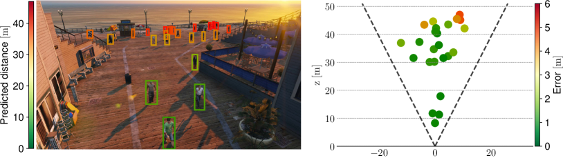
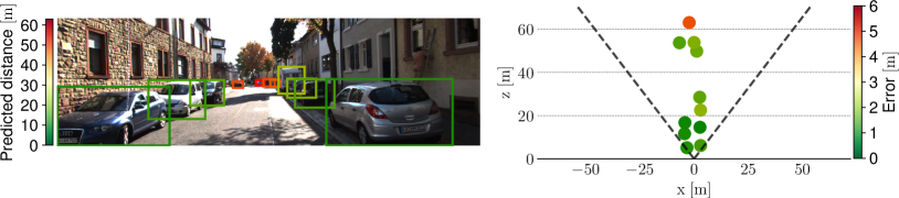
Figure 1: Qualitative results on MOTSynth (first row) and KITTI (second row). The left column shows bounding boxes and predicted distances, while the right column represents the same image in bird’s eye view. The color-coded circles indicate the error magnitude (best seen in colors).

Among past and novel challenges, the Computer Vision community has a long-standing commitment to estimating the third dimension. Namely, the goal is to estimate the distance of a target object from the camera (or observer) when projected onto the image plane, particularly in the context of monocular images. In this respect, humans continuously practice such a capability in everyday life. For example, when approaching a stop sign, the driver visually assesses the remaining distance to the sign and adjusts the car’s velocity accordingly. However, distance estimation through human perception is often rough and qualitative. Moreover, its precision depends on the skills of the subject and on its health status, which can be altered by the consumption of drugs and alcohol. Additionally, external factors such as high vehicle speed, the terrain [46], or adverse weather conditions can further worsen distance perception.

Due to the struggles of human perception, the development of machine vision has enabled the automation of tasks involving the precise estimation of distances and dimensions. Pioneer works accomplished it with the pinhole model, through which one can relate the image plane to the physical space by the standard projective transformation. Unfortunately, such an approach is viable only in static scenarios – which provide the camera model a priori – and suffers from radial lens distortion, hindering the estimation of the distance for objects located far from the center.

Modern approaches rely on additional geometric constraints or data-driven strategies. Based on that, per-object distance estimators can be broadly divided into two main categories: geometric and feature-based methods. The former [18, 19, 47] assumes that objects of the same class (e.g., pedestrians) have consistent sizes. Under such a hypothesis, these methods can exploit projective transformations to approach the task. Namely, it involves regressing the relationship, expected to be roughly linear, between the visual size of an object (such as the height of its bounding box) and its distance. Unfortunately, the assumption mentioned above does not hold in practice: in real-world scenarios, the dimensions of objects may vary significantly (e.g., from children to adults).

In contrast, feature-based approaches [51, 23, 29, 37] incorporate supplementary visual information regarding the target objects and the context of the scene. This is achieved by inputting the entire monocular image into a global encoder (e.g., a Convolutional Neural Network (CNN) [45, 20]) and retaining the activation of the last convolutional block; on top of that, techniques based on Region of Interest (RoI) are used to provide a spatially consistent and fixed-size feature vector for each target object. These approaches can reach a more holistic understanding of the scene, as they leverage local information and the spatial relations between the target and other reference objects of the scene [29].

While existing feature-based approaches avoid the shortcomings of the geometric ones, they also come with several architectural drawbacks that are peculiar to CNNs:

• The large receptive field of CNNs could wipe out the fine-grained information tied to the target object; there are no trivial ways to limit the receptive field’s growth.

• The pooling layers of CNNs downscale the resolution of the feature maps (e.g., by a factor of $32$ in ResNets). Unfortunately, it does so to the extent that smaller bounding boxes (allegedly, long-range objects, Fig. 1) cover only sub-pixel activation areas in latent space.

• The bottleneck design of CNNs tends to disregard the spatial relations between the parts and the whole. While it could benefit tasks such as classification, the task at hand demands the learner to develop a hidden belief regarding the mutual distances between nearby objects. Notably, spatial relations play an essential role also in human perception, as stated by the adjacency principle [17]. Indeed, an object’s apparent size or position in the field of view is determined by the size or distance cues between it and adjacent objects.

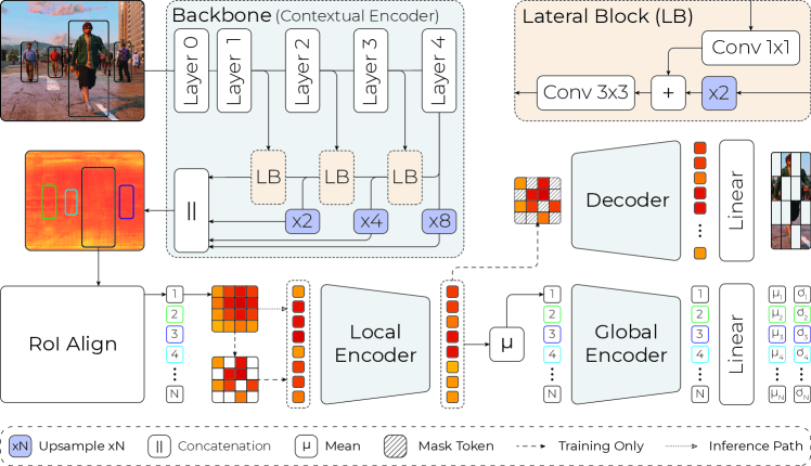
Figure 2: Overview of DistFormer. Initially, we feed the RGB frame $\mathbf{x}$ through a classical backbone to obtain an informative feature map. Successively, a RoIAlign operation extracts a feature vector for each object in the image, which is then split into tokens and processed by the Local Encoder, extracting intra-object characteristics. During training, we mask $k\%$ of the tokens and use a decoder to reconstruct the missing ones. Afterward, the Global Encoder extracts strong scene-level object relations. Finally, an MLP predicts a Gaussian, modeling the distance and its uncertainty.

Our work addresses the limitations above by proposing DistFormer (Fig. 2), a hybrid architecture combining CNNs and Transformer layers [48]. While still feature-based, our proposal can effectively exploit local and global information without giving up the depth of the visual encoding. The first part of DistFormer builds upon a Contextual Encoder network, that is a CNN equipped with additional layers based upon Feature Pyramid Networks [30] and allow our method to extract high-level representations that retain fine-grained details.

In a second stage, we extract per-object representations and pass them to two transformer-based encoders, which focus respectively on local cues and global relations. In more detail, the former one – the Local Encoder – performs self-attention between patches of the same object, disregarding information from other objects. Such a module aims at further enforcing the local visual reasoning and encouraging the extraction of fine-grained details; to do so, it receives an additional self-supervised training signal named Auxiliary Reconstruction Task (ART), whose design follows the Masked Image Modeling (MIM) paradigm [2]. Differently, the final component – i.e., the Global Encoder – aims at encoding spatial and global relations explicitly; we achieve it by carrying out self-attention among representations from distinct objects.

We validated the proposed approach by conducting extensive experiments on the real-world datasets KITTI [13] and NuScenes [5], and the synthetic large-scale MOTSynth [11]. Our findings show that our approach surpasses the state-of-the-art by a wide margin. In addition, we show that ART enhances transfer learning from synthetic pretraining. In fact, by performing a zero-shot test on KITTI and NuScenes (see Sec. 5), our approach – under its self-supervised component – surprisingly allows for better generalization, even with different intrinsic camera parameters.

We remark the following contributions: i) We propose a novel hybrid architecture that effectively combines CNNs and Transformer layers. This architecture strikes a balance between local and global information, addressing limitations in existing feature-based methods; ii) We introduce an innovative self-supervised component termed ART within the Local Encoder. This task enhances object-specific feature learning and encourages each object-specific feature vector to be highly informative, focusing on the object of interest. The ART enforces localized, detailed understanding, boosting the model’s performance; iii) We employ a Global Encoder module that refines local representations by learning mutual relations between objects in the scene.

2 Related Works

Object Distance Estimators. Estimating object distances from a single RGB image (i.e., monocular distance estimation) is a crucial task for many computer vision applications [1, 15, 40, 16, 39, 28, 51, 19]. One of the approaches to this task is to perform per-object distance estimation. Early works leverage the object’s geometry to find its distance. However, these works did not take into account any visual features. Among these works, the Support Vector Regressor (SVR) [18] finds the best-fitting hyperplane given the geometry of the bounding boxes. The Inverse Perspective Mapping (IPM) [36, 43] improves results by adopting an iterative approach that converts image points to bird’s-eye view coordinates. Nevertheless, this method introduces distortion on the image, making predicting distance for objects that are either distant or on curved roads challenging.

Successive methods [19, 18] exploit the object bounding box to infer its geometry through deep neural networks, effectively improving upon pure algorithmic techniques. The distance regressors of these deep methods solely focus on the bounding boxes’ geometry, similar to previous works. These approaches are limited when the target objects are of different classes e.g., vehicles and people. A car and a person with similar bounding boxes will have very different distances from the camera. The same also holds for an adult and a child. Zhu et al. [51] has made a notable improvement by introducing a structure inspired by Faster R-CNN [42] and extracting visual features with a RoIPool [14] operation. This approach captures significant visual features, which the distance regressor then uses to make precise predictions about the distances of objects. More recently, DistSynth [37] leverages multiple frames from a sequence to consistently predict distances over time.

A different approach in this field is monocular per-pixel depth estimation [10, 16, 28, 39], where the goal is to predict a depth map starting from a single RGB image. In [10], the authors propose employing two deep networks, one for coarse global predictions and one to refine such predictions locally. More recently, [28] used multi-resolution depth maps to construct the final map. However, these works have a high computational cost and are difficult to implement in a real-time system such as autonomous driving. Moreover, translating the depth map into object distance is nontrivial due to occlusions and the looseness of bounding boxes.

Transformers, initially introduced in [48] to address machine translation challenges, revolutionized the field by treating individual words as tokens. Dosovitskiy et al. [8] expanded their application beyond linguistic domains, introducing the Vision Transformer (ViT), adapting transformers to computer vision by segmenting images into patches and treating them as tokens.

In a further advancement, He et al. proposed the masked autoencoder (MAE) approach [22] to enhance training efficiency and downstream task accuracy. This approach involves pre-training a standard ViT encoder using a randomly selected subset of image patches. A shallow ViT encoder, acting as a decoder, reconstructs the missing input image patches. This technique accelerates the training process and improves performance in subsequent tasks.

3 Method

Overview. We herein discuss the architecture of the deep distance estimator and the objective function optimized to obtain the parameters $\theta_{[\cdot]}$. The overall architecture, depicted in Fig. 2, comprises three main building blocks:

1. a convolutional backbone $f(\mathbf{x};\theta_{f})$ extracting global visual features from a monocular image $\mathbf{x}$ (see Sec. 3.1);

2. a Local Encoder $LE(f(\cdot);\theta_{L})$, which operates at the object level. Such a module receives an additional self-supervised training signal based on that of masked autoencoders (see Sec. 3.2);

3. a Global Encoder $GE(LE(\cdot);\theta_{G})$ which uses scene-level reasoning based on the encoder output to predict the distance of the objects (see Sec. 3.3).

3.1 Contextual Encoder

We feed our backbone $f$ with a raw (i.e., without distortion correction) RGB frame $\mathbf{x}\in\mathbb{R}^{C\times H\times W}$ where $C$ is the number of channels and $\left(H,W\right)$ are the frame resolution.

We base our backbone architecture on convolutional residual networks [20], employing a ConvNeXt [33] pre-trained on ImageNet-22k. Such convolutional networks usually comprise pooling layers that progressively reduce the feature map’s resolution. While providing some advantages for classification tasks (e.g., translation invariance, high-level reasoning etc.) [25], we argue that pooling layers and other resolution reduction techniques would damage the task of distance estimation. For example, the portion of the feature map containing distant objects could consist of only a few pixels or even just one, resulting in a more coarse successive extraction of features.

We address these shortcomings leveraging a Feature Pyramid Network (FPN) [30], as in [37, 27, 6, 50]. In a nutshell, an FPN-based network incorporates two branches: a standard forward branch for downsampling feature maps and a backward branch that progressively upscales the output of the forward pass. The backward branch takes the output of the forward pass and progressively upscales it through Lateral Blocks (LB). Finally, feature maps from each LB are upsampled to the dimension of the largest one and concatenated into a single feature map containing representative visual features (see Backbone gray block in Fig. 2).

3.2 Local Encoder

The features processed by our backbone contain information to predict the distance of the objects of interest. We apply the RoIAlign [21] operation to have constant-length vectors and to extract the portion of the feature map representing the target object. This operation yields feature vectors $\mathcal{F}_{i}\ {\in}\ \mathbb{R}^{c\times h\times w}$ with $i\,{:=}\,\{1,\ldots,N\}$ where $N$ is the number of bounding boxes in the image, $c$ represents the number of channels of the feature map and $(h,w)$ are the dimensions of the RoI quantization. Compared to RoIPool, commonly used in this task [51, 29], RoIAlign avoids misalignments thanks to a more accurate interpolation strategy.

To better encode the information of the target object, we employ a Local Encoder (LE) module. First, we collapse the feature map of each object $\mathbb{R}^{c\times(h\times w)}\to\mathbb{R}^{c\times(h\cdot w)}$, treating each pixel of the activation map as a token. Then, the LE, based on a ViT encoder, will perform self-attention on the object’s tokens. Such operation extracts informative intra-object features and lets the model focus on the most critical portions of the objects, e.g., not occluded.

Furthermore, we adopt a self-supervised approach during the training phase: an Auxiliary Reconstruction Task (ART). Specifically, as in masked autoencoders [22], we feed the encoder with only a percentage of the input tokens, also allowing for ease of the computational cost. Subsequently, we employ a decoder network $D(\cdot,\theta_{D})$ to reconstruct the input image cropped by the bounding box. The masked tokens are substituted by learned masked tokens, while the unmasked tokens are taken directly from the encoder output. Finally, the ART objective is applied only to the masked tokens. This approach forces each token to be as informative as possible and to focus on the object of interest.

The resulting objective is:

$$\mathcal{L}_{\mathrm{ART}}=\mathbb{E}_{(\mathbf{\mathbf{x}}_{i},\mathcal{F}_{i})\in\mathbf{\mathcal{X}}}\left[||D(LE(\mathcal{F}_{i},\theta_{LE}),\theta_{D})-\mathbf{x}_{i}||_{2}^{2}\right],$$ (1)

where $\mathbf{x}_{i}$ is the RoI cropped from the original image of the $i$-th object and $\mathbf{\mathcal{X}}$ the whole set of detected objects.

3.3 Global Encoder

The LE yields $h\cdot w$ tokens $\in\mathbb{R}^{c}$ for each bounding box. We employ global average pooling along the token axis to distill a comprehensive representation, as in [32]. The Global Encoder (GE), which builds upon the ViT architecture, enhances the understanding of inter-object relationships of the scene. Through a self-attention operation, each token can assimilate insights from other objects, even those that may be occluded or occlude the target object.

The result is a token $\in\mathbb{R}^{c}$ for each bounding box containing robust intra-object features infused by the LE and a broad inter-object knowledge given by the GE. Afterward, we process each token with a standard Multi-Layer Perceptron to obtain each object’s predicted distance.

3.4 Training objective

Given the intrinsic ambiguity of the task at hand due to the characteristics variation of each object, e.g., human height, we opt for predicting a Gaussian distribution over the expected distance than a punctual estimation. The mean of the distribution represents the distance, while its variance is the model aleatoric uncerteainty [3, 7], which refers to the inherent noise contained in the observations. To do so, the latter part of the network outputs two scalars for each object; on top of them, the supervised part of the overall training signal can be carried by lowering the Gaussian Negative Log Likelihood (GNLL) [38] of ground-truth distances.

The final objective is given by Eq. 1 and the GNLL:

$$\mathcal{L}=\alpha\mathcal{L}_{\mathrm{ART}}+\mathcal{L}_{\mathrm{GNLL}},$$ (2)

where $\alpha$ is a hyper-parameter balancing the importance of the ART loss function.

4 Experiments

	$\delta_{<1.25}\uparrow$	ABS$\downarrow$	SQ$\downarrow$	RMSE$\downarrow$	RMSElog$\downarrow$
Cars
SVR [18]	34.50%	149.4%	47.7	18.97	1.49
IPM [47]	70.10%	49.70%	1290	237.6	0.45
DisNet [19] *	70.21%	26.49%	1.64	6.17	0.27
Zhu et al. [51]	84.80%	16.10%	0.61	3.58	0.22
CenterNet [9]	95.33%	8.70%	0.43	3.24	0.14
PatchNet [35]	95.52%	8.08%	0.28	2.90	0.13
Jing et al. [23]	97.60%	6.89%	0.23	2.50	0.12
DistFormer	94.32%	9.97%	0.22	2.11	0.13
Pedestrian
SVR [18]	12.90%	149.9%	34.56	21.68	1.26
IPM [47]	68.80%	34.00%	543.2	192.18	0.35
DisNet [19] *	93.24%	7.69%	0.27	3.05	0.12
Zhu et al. [51]	74.70%	18.30%	0.65	3.44	0.22
DistFormer	98.15%	5.67%	0.08	1.26	0.09
Cyclists
SVR [18]	22.60%	125.1%	31.61	20.54	1.21
IPM [47]	65.50%	32.20%	9.54	19.15	0.37
DisNet [19] *	84.42%	12.13%	0.96	7.09	0.19
Zhu et al. [51]	76.80%	18.80%	0.92	4.89	0.23
DistFormer	95.62%	8.01%	0.25	3.09	0.11
All
SVR [18]	37.90%	147.2%	90.14	24.25	1.47
IPM [47]	60.30%	39.00%	274.7	78.87	0.40
DisNet [19] *	69.83%	25.30%	1.81	6.92	1.32
Zhu et al. [51]	48.60%	54.10%	5.55	8.74	0.51
+ classifier	62.90%	25.10%	1.84	6.87	0.31
DistFormer	93.67%	10.39%	0.32	2.95	0.15
- W/out ART	93.43%	10.61%	0.34	3.17	0.15

Table 1: Experimental comparison on KITTI, following the setting in [51]. ( * ) our implementation.

	$\delta_{<1.25}\uparrow$	ABS$\downarrow$	SQ$\downarrow$	RMSE$\downarrow$	RMSElog$\downarrow$
NuScenes
SVR [18]	32.49%	57.65%	10.48	19.18	4.017
DisNet [19]	76.60%	18.47%	1.646	8.270	0.228
Zhu et al. [51]	84.54%	14.95%	1.244	7.507	0.245
DistFormer	95.33%	8.13%	0.533	5.092	0.146
- W/out ART	91.10%	11.16%	0.807	6.363	0.165
MOTSynth
SVR [18]	26.08%	54.67%	6.758	12.61	0.588
DisNet [19]	94.15%	8.73%	0.266	2.507	0.123
Zhu et al. [51]	98.71%	4.40%	0.116	2.131	0.065
DistSynth [37]	99.13%	3.71%	0.073	1.567	0.142
Monoloco [3]	99.69%	3.59%	0.064	1.488	0.167
DistFormer	99.70%	2.81%	0.037	1.081	0.043
- W/out ART	99.31%	3.36%	0.046	1.152	0.053

Table 2: Performance comparison on the NuScenes and MOTSynth datasets.

4.1 Datasets

KITTI [13] is a well-known benchmark for autonomous driving, object detection, visual odometry, and tracking. The object detection benchmark includes $7481$ training and $7518$ test RGB images with the corresponding LiDAR point clouds. A total of $80\,256$ labeled objects, including pedestrians, cars, and cyclists, are present. Following the convention proposed in [6], we divide the train set into training and validation subsets with $3712$ and $3768$ images, respectively. We obtain ground truth distances for each object from the point cloud, following the strategy in [51] (see supplementary materials).

NuScenes [5] is a large-scale multi-modal dataset with data from 6 surround-view cameras, 5 radars, and 1 LiDAR sensor. It comprises $1000$ driving scenes collected from urban environments, featuring 1.4M annotated 3D bounding boxes across 10 object categories. Following [29], we consider the object’s center as the ground truth distance.

MOTSynth [11] is a large synthetic dataset for pedestrian detection, tracking, and segmentation in an urban environment comprising $764$ videos of $1800$ frames with $190$ test sequences and $574$ train sequences, with different weather conditions, lighting, and viewpoints. Among other annotations, MOTSynth provides 3D coordinates of skeleton joints. Given its lower probability of occlusion, we select the distance of the head joint as the ground truth value.

Pseudo Long-Range KITTI and NuScenes [29] are subsets designed for assessing the performance of distance estimation models on long-range objects (i.e., beyond $40$ meters). The KITTI subset, comprises $2181$ training images and $2340$ validation images, containing $4233$ and $4033$ vehicles, respectively. The NuScenes subset, instead, includes $18\,926$ training images with $59\,800$ target vehicles and $4017$ validation images with $11\,737$ target vehicles.

	Dataset (Long Range)		Higher is better			Lower is better
		LiDAR	$<5\%$	$<10\%$	$<15\%$	ABS	SQ	RMSE	RMSElog
SVR [18]	KITTI	-	39.1%	65.9%	79.0%	10.2%	1.38	9.5	0.166
DisNet [19]	KITTI	-	37.1%	65.0%	77.7%	10.6%	1.55	10.4	0.181
Zhu et al. [51]	KITTI	-	39.4%	65.8%	80.2%	8.7%	0.88	7.7	0.131
Zhu et al. [51]	KITTI	✓	41.1%	66.5%	78.0%	8.9%	0.97	8.1	0.136
R4D [29]	KITTI	✓	46.3%	72.5%	83.9%	7.5%	0.68	6.8	0.112
Ours	KITTI	-	56.3%	88.3%	97.3%	5.2%	0.22	3.3	0.064
SVR [18]	NuScenes	-	33.0%	58.0%	74.0%	10.9%	1.56	10.7	0.166
DisNet [19]	NuScenes	-	29.5%	58.6%	75.0%	10.7%	1.46	10.5	0.162
Zhu et al. [51]	NuScenes	-	40.3%	66.7%	80.3%	8.4%	0.91	8.6	0.121
Zhu et al. [51]	NuScenes	✓	37.7%	63.5%	77.2%	9.2%	1.06	9.2	0.132
R4D [29]	NuScenes	✓	44.2%	71.1%	84.6%	7.6%	0.75	7.7	0.110
Ours	NuScenes	-	47.3%	75.4%	88.6%	7.3%	0.65	6.8	0.104

Table 3: Comparison between different approaches on the Pseudo Long-Range KITTI and NuScenes datasets.

4.2 Experimental details

Metrics. We rely on popular metrics of per-object distance estimation [10, 51, 12, 44, 31], such as the $\tau$-Accuracy ($\delta_{\tau}$) [26] (i.e., the maximum allowed relative error), the percentage of objects with relative distance error below a certain threshold ($<5\%$, $<10\%$, $<15\%$) [29] and classical error distances [51]: absolute relative error (ABS), square relative error (SQ), and root mean squared error in linear and logarithmic space (RMSE and RMSE_log). For brevity, we report the corresponding equations in the supplementary materials.

Evaluation Setting.   The evaluation adheres to the widely adopted benchmark [51, 19, 23, 37, 29] wherein the model is fed with ground truth bounding boxes (or poses). Namely, the model is supplied with ground truth bounding boxes (or poses) during inference, along with the input image. Such an approach proves instrumental in disentangling the detector’s performance from that of the distance estimator.

Implementation Details. The RoIAlign window is set to $8\times 8$. During training, 50% of tokens are fed into the Local Encoder $LE(f(\cdot);\theta_{E})$, while the entire set is processed during inference. The LE comprises the last 6 layers of a pre-trained ViT-B/16, and the Decoder $D$ and the Global Encoder GE are 2-layer transformer encoders. Training occurs end-to-end on an NVIDIA 2080 Ti for 24 hours on NuScenes and MOTSynth and 6 hours on KITTI. Early stopping is applied to mitigate overfitting.

Since we are not interested in a dense prediction, i.e., a depth map, but solely in the object-specific distance, we force the model to focus on a restricted set of locations. To achieve this, we augment the input RGB frame by concatenating an extra channel representing each bounding box’s center using a Gaussian signal. We report further implementation details in the supplementary materials.

4.3 Comparison with State-of-the-Art

Baselines. Our comparison includes various approaches:

Backbone	Local Encoder	Global Encoder	$\delta_{<1.25}$ $\uparrow$	ABS $\downarrow$	SQ $\downarrow$	RMSE $\downarrow$	RMSElog $\downarrow$
ViT-B/16	✓	Transformer	92.78%	7.88%	0.460	3.973	0.123
	+ART	Transformer	94.90%	6.81%	0.316	3.473	0.104
ResNet34	✓	Transformer	98.93%	4.14%	0.107	2.078	0.062
	+ART	Transformer	98.94%	4.36%	0.094	1.826	0.064
ResNet34-FPN	-	-	98.91%	4.45%	0.102	1.975	0.064
	✓	-	99.53%	3.44%	0.056	1.363	0.051
	-	Transformer	99.59%	3.30%	0.054	1.302	0.050
	✓	Transformer	99.70%	3.15%	0.050	1.302	0.047
	+ART	GAT	99.51%	3.49%	0.049	1.213	0.051
	+ART	Transformer	99.70%	3.00%	0.040	1.146	0.044
ConvNeXt-S-FPN	-	-	99.31%	3.38%	0.055	1.289	0.051
	✓	-	99.34%	3.41%	0.055	1.275	0.053
	-	Transformer	99.43%	3.38%	0.052	1.236	0.053
	✓	Transformer	99.31%	3.36%	0.046	1.152	0.053
	+ART	-	99.38%	3.31%	0.053	1.290	0.050
	+ART	GAT	99.63%	3.26%	0.048	1.221	0.049
ConvNeXt-S-FPN	+ART	Transformer	99.70%	2.81%	0.037	1.081	0.043

Table 4: Ablation of the backbone and proposed modules on the MOTSynth dataset.

• Geometric methods. SVR [18] learns the distribution of the height and width of the bounding boxes while IPM [47] approximates a transformation matrix between a normal RGB image and its bird’s-eye view image. Disnet [19] employs a deep approach to process a feature vector composed of normalized bounding box features and their class priors. Monoloco [3] exploits the human pose to infer the distance.

• Feature-based methods. Zhu et al. [51], CenterNet [9], PatchNet [35], Jing et al. [23], and DistSynth [37] exploit visual features extracted by a CNN.

In our NuScenes and MOTSynth experiments, we use the same backbone, both for DistFormer and other methods. We train all methods with ground truth bounding boxes except Monoloco [3], which we trained with ground truth human poses.

Tables 1 and 2 present the results of our approach and previous work. Results on KITTI are extracted from their respective papers, while for NuScenes and MOTSynth, we implemented and conducted experiments from scratch. While non-deep geometric methods perform poorly, deep ones perform much better, proving a correlation between the object size and distance from the camera. In addition, visual feature methods improve upon geometric ones, especially on KITTI, which features multiple target classes, showing that more than geometric features are needed for an accurate distance prediction. Our approach achieves state-of-the-art results on the KITTI dataset across all classes except for cars (see Tab. 1). It is noteworthy that methods surpassing our approach are tailored specifically for the car class or designed for multi-frame scenarios (e.g., Jing et al. [23]). In contrast, our approach generalizes over all classes without additional objectives.

The NuScenes dataset presents much more data and unique challenges with its diverse scenes, dynamic scenarios, complex traffic situations, and a maximum distance of over 150 meters. Despite these challenges, our proposed approach demonstrates robust performance, achieving state-of-the-art results across all metrics as depicted in Tab. 2.

Finally, the MOTSynth dataset exclusively focuses on the pedestrian class; its extensive range of landscapes, viewpoints, and visual characteristics makes it a comprehensive benchmark. In Tab. 2, our proposed approach demonstrates significant improvements, outperforming existing methods across all metrics. Notably, we achieve a remarkable $-27$% reduction in RMSE for Monoloco and an even more impressive $-49$% reduction for the Zhu et al. approach.

Long-Range Distance Estimation. DistFormer proves effective also on KITTI and NuScenes long-range benchmarks (Tab. 3), showcasing accurate perception of distant objects. The hyperparameters used for these datasets are the same for the entire datasets (Tabs. 1 and 2), and no additional tuning has been carried out.

While R4D [29] was explicitly designed for the long-range task, our results show that our approach is more versatile as it performs well on both short- and long-range objects with no additional input sensor data (i.e., LiDAR as R4D does at inference). In this respect, we argue that it can be ascribed to the different mechanisms employed to gather global information: R4D builds upon the graph of pair-wise relationships between the target object and its references; we differently leverage self-attention to encode global relations among the whole set of objects in the scene.

5 Model Analysis

Ablation studies. Tab. 4 depicts the comparison between different backbones and the ablation of the LE and GE modules, discussed in the following.

Feature extraction. We explore the impact of different backbones on the final performance. Initially, we remark that using a ViT-B/16 as the backbone is infeasible at full resolution (i.e., $720\times 1280$) due to its memory footprint. Hence, we adopt the standard resolution of $224\times 224$. As suggested by the first two rows of Tab. 4, replacing the convolutional backbone with a ViT-B/16 reduces performance, proving that a higher input resolution benefits the task. Moreover, using ResNet without the FPN module worsens the results, indicating that multi-scale features and the larger feature map play a role in accurately predicting distances.

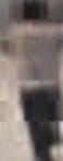
Figure 3: ART module reconstructions on MOTSynth.

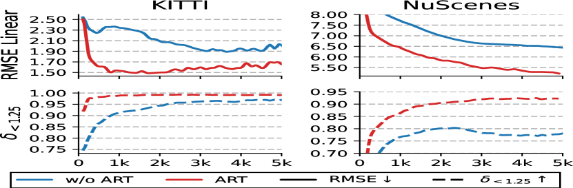
Figure 4: Fine-tuning results from MOTSynth to KITTI and NuScenes for the Pedestrian class with varying numbers of training samples.

Local Encoder. The experiments on both ResNet34-FPN and ConvNeXt-S-FPN highlight the role of the LE to process local cues. Indeed, its application (✓) improves across all metrics. Moreover, the self-supervised ART module further improves results (rows marked with +ART) by regularizing the model features to preserve visual cues. The impact of the ART module is depicted in Fig. 3, where it demonstrates a tendency to eliminate non-essential visual features, such as clothes colors and aligning objects towards a more prototypical representation.

Global Reasoning. Discarding the GE leads to a remarkable performance drop, confirming the ideas discussed in Sec. 3.3. Moreover, to assess the merits of self-attention layers, we provide further results using a Graph Attention Network (GAT) [49, 4] as Global Encoder. We note that applying GAT results in improvements w.r.t. not using any Global Encoder. However, the transformer self-attention consistently outperforms GAT, underscoring the efficacy of our chosen mechanism for global reasoning.

Synth-to-Real transfer. We herein present a cross-dataset evaluation to assess the ability of DistFormer to capture robust and general features with high synth-to-real transfer potential. Initially, we train our model on the MOTSynth dataset, with and without the ART objective; then, we shift to KITTI and NuScenes, evaluating performance on instances of pedestrians (i.e., the only one present in all datasets) under two settings: zero-shot, without any model refinement on the target dataset, and with fine-tuning.

From the zero-shot results in Tab. 5, we notice an outstanding generalization capability of our model trained on synthetic data, even surpassing previous works trained explicitly on KITTI, meaning that DistFormer can extract highly informative features for the task at hand. Moreover, we acknowledge that the intrinsic camera parameters of the different datasets are very different, as can also be seen from the FOV comparison in Fig. 1. Nevertheless, the ability to perform well without distortion correction and different camera parameters shows that our model strongly relies on global cues and can account for visual distortion. Finally, as suggested by Fig. 4, the ART module provides more reliability and sample efficient training.

ART	$\delta_{<1.25}{\uparrow}$	ABS$\downarrow$	SQ$\downarrow$	RMSE$\downarrow$	RMSElog$\downarrow$
zero-shot
MOTSynth $\,\to\,$ KITTI
-	70.44%	18.51%	0.56	2.95	0.26
✓	83.57%	17.56%	0.47	2.87	0.17
MOTSynth $\,\to\,$ NuScenes
	44.07%	20.74%	1.93	9.10	0.26
✓	46.70%	19.94%	1.74	8.74	0.25
fine-tuning
MOTSynth $\,\to\,$ KITTI
-	97.58%	6.05%	0.12	1.89	0.09
✓	99.16%	5.42%	0.12	1.48	0.07
MOTSynth $\,\to\,$ NuScenes
-	80.42%	15.62%	1.10	6.27	0.18
✓	92.23%	10.28%	0.64	5.22	0.13

Table 5: Comparison of ART contribute over zero-shot and fine-tuning synth-to-real transfer.

	Time	FLOPs	Params	RMSE
Zhu et al. [51]	61.9 ms	320 G	110 M	3.33
DistFormer	67.6 ms	380 G	196 M	2.87
+ mask 30%	66.5 ms	360 G	196 M	2.89
+ mask 50%	65.2 ms	345 G	196 M	2.91
+ mask 80%	64.4 ms	330 G	196 M	3.14

Table 6: Computational cost comparison analysis on KITTI (all classes). All models use the ConvNeXt backbone.

Computational analysis. While the proposed architecture comprises different modules, and the self-attention module is applied to each bounding box, the computational cost remains contained. Specifically, the Zhu et al. model requires, on average, $61.9$ ms per frame, while our DistFormer only adds $\approx$ $6$ ms to the inference time as depicted in Tab. 6. We further expand such an analysis by building upon an interesting gift from Masked Autoencoders: they allow for faster inference by simply leveraging random masking at inference time. By doing so, our approach still yields good estimates with reduced wall-clock times.

6 Conclusion

We propose DistFormer, a novel and reliable approach for per-object distance estimation. It includes a local reasoning module performing self-attention between patches of the same object, which seeks to capture an object’s local and peculiar visual attributes (e.g., shape and texture). Moreover, DistFormer comprises a global module, exploiting self-attention between objects to deliver scene-aware predictions. Overall, we have shown that an additional self-supervised signal greatly benefits the generalization capabilities of the model and synth-to-real knowledge transfer.

Supplementary Material

Appendix A Bounding Box Prior Through Centers Mask

To provide an additional signal on the objects, we feed the backbone with a further channel representing the centers of the bounding boxes. Specifically, we construct a heatmap $h$ where we apply a fixed variance Gaussian over each center. Formally, given the bounding box $\mathbf{t}^{k}=(t^{k}_{x},t^{k}_{y},t^{k}_{w},t^{k}_{h})$, with $k\in\{1,\ldots,K\}$, where $K$ is the number of the bounding boxes in the frame, and the bounding box tuple represents the $x$ and $y$ coordinates of the top left corner $(t^{k}_{x},t^{k}_{y})$ and its width and height $(t^{k}_{w},t^{k}_{y})$, the heatmap $h^{k}$ for a generic bounding box centered in $\mathbf{c}^{k}=(c^{k}_{x},c^{k}_{y})=(t^{k}_{x}+t^{k}_{w}/2,t^{k}_{y}+t^{k}_{h}/2)$ is given by:

$$h^{k}(\mathbf{u})=\exp{\left(-\frac{||\mathbf{u}-\mathbf{c}^{k}||^{2}}{\sigma^{2}}\right)},$$ (A)

where $\mathbf{u}$ is the generic $(x,y)$ location of the heatmap. In a multi-object context, where centers may overlap, we aggregate the heatmaps $h^{k}$ into a single heatmap $h$ with a max operation:

$$h=\max_{k}\{h^{k}(\mathbf{u})\}.$$ (B)

In Tab. A, we present the ablation results of the centers’ heatmap. In particular, we show that adding such a signal leads to a slight improvement in all metrics.

Centers	$\delta_{<1.25}$ $\uparrow$	ABS $\downarrow$	SQ $\downarrow$	RMSE $\downarrow$	RMSElog $\downarrow$
	99.52%	3.07%	0.051	1.266	0.048
✓	99.70%	2.81%	0.037	1.081	0.043

Table A: Contribute of the centers mask.

Appendix B KITTI pre-processing

config	MOTSynth [11]	KITTI [13]	NuScenes [5]
ConvNeXt size	Small	Base	Small
input resolution	$720\times 1280$	$375\times 1242$	$900\times 1600$
optimizer	AdamW [24]	AdamW [24]	AdamW [24]
base learning rate	$1\text{\times}{10}^{-4}$	$5\text{\times}{10}^{-5}$	$5\text{\times}{10}^{-5}$
learning rate schedule	cosine annealing WR [34]	cosine annealing WR [34]	cosine annealing WR [34]
weight decay	$1\text{\times}{10}^{-5}$	$2\text{\times}{10}^{-5}$	$1\text{\times}{10}^{-5}$
ART weight	$\alpha=10$	$\alpha=20$	$\alpha=10$
ART masking ratio	$50\%$	$50\%$	$50\%$
optimizer momentum	$\beta_{1},\beta_{2}=(0.9,0.999)$	$\beta_{1},\beta_{2}=(0.9,0.999)$	$\beta_{1},\beta_{2}=(0.9,0.999)$
batch size	$2$	$4$	$2$
dist loss delay epochs	$0$	$20$	$0$
dist loss warmup epochs	$11$	$10$	$0$
augmentation	RandomLRFlip ($p=0.5$)	RandomLRFlip ($p=0.5$)	RandomLRFlip ($p=0.5$)
	ColorJitter ($p=0.25$)
	GaussianBlur ($p=0.25$)
	RandomGrayscale ($p=0.2$)
	RandomAdjustSharpness ($p=0.5$)

Table B: DistFormer hyperparameters.

To obtain the ground truth annotation for the KITTI [13] dataset, we follow the setting proposed by Zhu et al. [51]. Specifically, for each object in the scene, we get all the point cloud points inside its 3D bounding box and sort them by distance. The chosen keypoint will be the n-th depth point where $n=0.1\cdot(\text{number of points})$. After that, we remove objects marked with the Don’t Care class and objects with a negative distance from the training set, which are objects behind the camera but still captured by the LiDAR.

Appendix C NuScenes pre-processing

We utilized the preprocessing methodology outlined in [29] for NuScenes [5]; specifically, we exploited the code provided by its authors to convert the dataset into the KITTI format. This conversion allows us to leverage existing KITTI-specific code. It is worth noting that, unlike KITTI, where we adhere to the configuration proposed by [51], for NuScenes, we adopt the Z component of the 3D bounding box’s center as the annotation.

Appendix D MOTSynth pre-processing

Since the MOTSynth [11] dataset was generated synthetically, its set of annotations covers all the pedestrians in the scene. On the one hand, we believe that such a variety could be beneficial and ensure good generalization capabilities; on the other hand, we observed that it hurts the performance, as some target annotations are highly noisy or extremely difficult for the learner. Thus we follow the filtering step from [37]. Specifically, the dataset contains annotations even for completely occluded people (e.g., behind a wall) or located very far from the camera (e.g., even at $100$ meters away). Hence, we discard these cases from the training and evaluation phases, performing a preliminary data-cleaning stage. Namely, in each experiment, we exclude pedestrians not visible from the camera viewpoint or located beyond the threshold used in [37] (i.e., $70$ meters).

Lastly, we sub-sample the official MOTSynth test set, keeping one out of 400 frames. This way, we avoid redundant computations and speed up the evaluation procedure.

Appendix E Metrics

In the following, we present the equations for the standard distance estimation metrics used in our work.

$$\delta_{\tau}:\text{Percentage of }d_{i}\text{ such that }\max\left(\frac{d_{i}}{d_{i}^{*}},\frac{d_{i}^{*}}{d_{i}}\right)=\delta_{\tau}<\tau$$

$$<\phi\%\text{-Accuracy}:\delta_{1+\phi}<1+\phi$$

$$\operatorname{ABS}:\frac{1}{N}\sum_{d\in N}\left(\left|d-d^{*}\right|/d^{*}\right)$$

$$\operatorname{SQ}:\frac{1}{N}\sum_{d\in N}\left(\left(d-d^{*}\right)^{2}/d^{*}\right)$$

$$\operatorname{RMSE}:\sqrt{\frac{1}{N}\sum_{d\in N}\left(\left(d-d^{*}\right)^{2}\right)}$$

$$\operatorname{RMSE}_{\log}:\sqrt{\frac{1}{N}\sum_{d\in N}\left(\left(\log d-\log d^{*}\right)^{2}\right)}$$

$$\operatorname{ALE}_{[\tau_{1}:\tau_{2}]}=\frac{1}{N}\sum\nolimits_{d\in N_{[\tau_{1}:\tau_{2}]}}\left|d-d^{*}\right|$$

where $d^{*}$ are the ground truth distances and $d$ the predicted distances.

Appendix F Implementation Details

The input of our contextual encoder, composed of a ConvNeXt and an FPN branch, is the full-resolution image. We extract the feature vectors of the objects from the feature map via ROIAlign [21] with a window of $8\times 8$. Successively, we split the feature map in tokens, then we randomly mask $50\%$ of the tokens and feed the unmasked ones to the Local Encoder (LE), which is composed of the last $6$ layers of a ViT-B/16 pretrained on ImageNet. The output of the LE is used both in the ART branch (during training only) and the distance regression branch. The ART Decoder and the Global Encoder are 2-layer transformer encoders with 8 heads. Fig. A depicts some reconstructions obtained with the ART module. We report in Tab. B the additional hyper-parameters for the different datasets.

	ALE $\downarrow$	ALOE $\downarrow$
Method	0m-100m	30%-50%	50%-75%	75%-100%
KITTI
Zhu et al. [51]	2.084	1.86	2.19	2.21
DistFormer	1.854	1.71	1.89	1.94
- W/o ART	1.909	1.76	2.00	2.12
MOTSynth
Zhu et al. [51]	1.127	1.29	1.44	1.57
DistSynth [37]	0.835	1.08	1.15	1.41
DistFormer	0.617	0.76	0.85	0.99
- W/o ART	0.675	0.81	0.88	1.07

Table C: ALOE comparison between our method and competitors on KITTI and MOTSynth. All model use the ConvNeXt backbone.

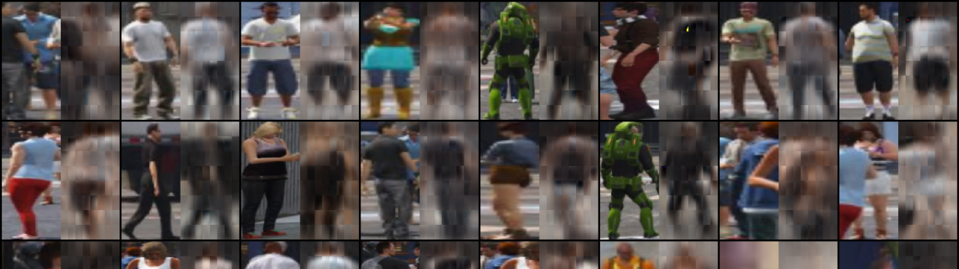
Figure A: Qualitative examples of the ART module output on MOTSynth. ART tends to remove aesthetic details, such as colors, costumes and decorations, while keeping the shape of people.

Appendix G Further Ablations

We present in Tab. D the ablations of the Local Encoder, Global Encoder, and ART module on the NuScenes dataset, following Sec. 5. Similar to what we found on the MOTSynth dataset, each module also improves the baseline on the NuScenes dataset, specifically with neither the Local Encoder nor the Global Encoder. Furthermore, such results show the importance of using the Transformer attention mechanism as a Global Encoder since the GAT considerably reduces the performance, even below the baseline. Finally, combining all the modules leads to more remarkable performance, especially on the RMSE metric.

Local Encoder	Global Encoder	$\delta_{<1.25}$ $\uparrow$	ABS $\downarrow$	SQ $\downarrow$	RMSE $\downarrow$	RMSElog $\downarrow$
-	-	94.77%	8.71%	0.587	5.459	0.135
✓	-	95.06%	8.37%	0.554	5.210	0.129
-	Transformer	94.98%	8.49%	0.558	5.341	0.131
✓	Transformer	95.20%	8.18%	0.532	5.243	0.134
+ART	-	95.14%	8.69%	0.568	5.170	0.132
+ART	GAT	93.38%	10.06%	0.697	5.738	0.146
+ART	Transformer	95.33%	8.13%	0.533	5.092	0.146

Table D: Ablation of proposed modules on the NuScenes dataset (using the ConvNeXt backbone).

Appendix H On the error in the presence of occlusions.

To provide further insight into DistFormer, we provide, in Tab. C, values for the ALOE metric proposed in [37]. We measure ALOE on KITTI based on the occlusion values provided by the dataset, namely, partially occluded (1), moderately occluded (2), and strongly occluded (3). We map these values in the 30%-50%, 50%-75%, and 75%-100% ranges. On MOTSynth, we follow the same setting as [37] and use the percentage of occluded joints to obtain the occlusion percentage of the objects. MOTSynth, known for its crowded scenarios, provides a realistic environment to evaluate our model performance with high and frequent occlusions. Unfortunately, NuScenes does not provide occlusion values; thus, no further study has been carried out on this dataset. Moreover, we cannot evaluate DistSynth [37] on KITTI as the sequence of frames is not long enough to match the requirements of such a method (i.e., 4 frames against the $8\times 5$ required).

In Tab. C Specifically, our method consistently outperforms all competitors over all ranges in both datasets. Moreover, we achieve a surprising ALOE below $1$ meter in all occlusion ranges in MOTSynth. We further expand the analysis by removing the ART module, showcasing a reduction in ALOE. Such a result proves that the ART module enforces the model to focus on the non-occluded portion of the target object.

Appendix I Evaluation using estimated bounding boxes

Method	$\delta_{<1.25}$ $\uparrow$	ABS $\downarrow$	SQ $\downarrow$	RMSE $\downarrow$	RMSElog $\downarrow$
DisNet [19]	70.24%	18.60%	1.006	5.633	0.237
Zhu et. al. [51]	93.90%	8.43%	0.200	2.382	0.129
DistFormer	94.60%	7.82%	0.165	2.114	0.122
Zhu et. al. [51] (GT)	-%	-%	-	-	-
DistFormer (GT)	94.68%	7.88%	0.163	2.075	0.120

Table E: Comparison with estimated detections on KITTI.

While the evaluation setting shown in Sec. 4.2 is used to disentangle the distance estimation capability from the detector performance, it can still be interesting to assess the performance of the proposed approach on noisy bounding boxes, i.e., those from a 2D object detector.

However, such an experiment comes with some criticalities, namely associating the detected bounding box with the correct ground truth distance. To effectively associate the bounding boxes, we use a bipartite matching algorithm with the IoU as the weight of the edges. Expressly, we set the IoU threshold to 0.7. We implement such a pipeline on the KITTI dataset using a fine-tuned YOLOv8 [41] detector. The association matches 59.7% of the ground-truth bounding boxes.

Accordingly, results on KITTI presented in Tab. E show that performances do not dramatically degrade in noisy input, and DistFormer consistently outperforms other methods.

Appendix J Bird’s-eye-view qualitatives

In the following, we show some qualitative results showcasing the effectiveness of DistFormer in estimating distances across KITTI, NuScenes, and MOTSynth datasets. These qualitative studies show our model’s efficacy at estimating distances in scenarios where even human responses fall short of approximation.

References

- Alhashim and Wonka [2018] Ibraheem Alhashim and Peter Wonka. High quality monocular depth estimation via transfer learning. arXiv preprint arXiv:1812.11941, 2018.
- Bao et al. [2021] Hangbo Bao, Li Dong, Songhao Piao, and Furu Wei. BEiT: BERT pre-training of image transformers. International Conference on Learning Representations Workshop, 2021.
- Bertoni et al. [2019] Lorenzo Bertoni, Sven Kreiss, and Alexandre Alahi. Monoloco: Monocular 3d pedestrian localization and uncertainty estimation. In IEEE International Conference on Computer Vision, 2019.
- Brody et al. [2022] Shaked Brody, Uri Alon, and Eran Yahav. How attentive are graph attention networks? In International Conference on Learning Representations Workshop, 2022.
- Caesar et al. [2020] Holger Caesar, Varun Bankiti, Alex H Lang, Sourabh Vora, Venice Erin Liong, Qiang Xu, Anush Krishnan, Yu Pan, Giancarlo Baldan, and Oscar Beijbom. nuscenes: A multimodal dataset for autonomous driving. In Proceedings of the IEEE conference on Computer Vision and Pattern Recognition, 2020.
- Chen et al. [2018] Long Chen, Haizhou Ai, Zijie Zhuang, and Chong Shang. Real-time multiple people tracking with deeply learned candidate selection and person re-identification. In IEEE International Conference on Multimedia and Expo, 2018.
- Der Kiureghian and Ditlevsen [2009] Armen Der Kiureghian and Ove Ditlevsen. Aleatory or epistemic? does it matter? Structural safety, 2009.
- Dosovitskiy et al. [2021] Alexey Dosovitskiy, Lucas Beyer, Alexander Kolesnikov, Dirk Weissenborn, Xiaohua Zhai, Thomas Unterthiner, Mostafa Dehghani, Matthias Minderer, Georg Heigold, Sylvain Gelly, Jakob Uszkoreit, and Neil Houlsby. An image is worth 16x16 words: Transformers for image recognition at scale. In International Conference on Learning Representations Workshop, 2021.
- Duan et al. [2019] Kaiwen Duan, Song Bai, Lingxi Xie, Honggang Qi, Qingming Huang, and Qi Tian. Centernet: Keypoint triplets for object detection. In IEEE International Conference on Computer Vision, 2019.
- Eigen et al. [2014] David Eigen, Christian Puhrsch, and Rob Fergus. Depth map prediction from a single image using a multi-scale deep network. Advances in Neural Information Processing Systems, 2014.
- Fabbri et al. [2021] Matteo Fabbri, Guillem Brasó, Gianluca Maugeri, Aljoša Ošep, Riccardo Gasparini, Orcun Cetintas, Simone Calderara, Laura Leal-Taixé, and Rita Cucchiara. Motsynth: How can synthetic data help pedestrian detection and tracking? In IEEE International Conference on Computer Vision, 2021.
- Garg et al. [2016] Ravi Garg, Vijay Kumar Bg, Gustavo Carneiro, and Ian Reid. Unsupervised cnn for single view depth estimation: Geometry to the rescue. In Proceedings of the European Conference on Computer Vision, 2016.
- Geiger et al. [2012] Andreas Geiger, Philip Lenz, and Raquel Urtasun. Are we ready for autonomous driving? the kitti vision benchmark suite. In Proceedings of the IEEE conference on Computer Vision and Pattern Recognition, 2012.
- Girshick [2015] Ross Girshick. Fast r-cnn. In IEEE International Conference on Computer Vision, 2015.
- Godard et al. [2017] Clément Godard, Oisin Mac Aodha, and Gabriel J Brostow. Unsupervised monocular depth estimation with left-right consistency. In Proceedings of the IEEE conference on Computer Vision and Pattern Recognition, 2017.
- Godard et al. [2019] Clément Godard, Oisin Mac Aodha, Michael Firman, and Gabriel J Brostow. Digging into self-supervised monocular depth estimation. In Proceedings of the IEEE conference on Computer Vision and Pattern Recognition, 2019.
- Gogel [1963] Walter C Gogel. The visual perception of size and distance. Vision Research, 1963.
- Gökçe et al. [2015] Fatih Gökçe, Göktürk Üçoluk, Erol Şahin, and Sinan Kalkan. Vision-based detection and distance estimation of micro unmanned aerial vehicles. Sensors, 2015.
- Haseeb et al. [2018] Muhammad Abdul Haseeb, Jianyu Guan, Danijela Ristic-Durrant, and Axel Gräser. Disnet: a novel method for distance estimation from monocular camera. 10th Planning, Perception and Navigation for Intelligent Vehicles (PPNIV18), IROS, 2018.
- He et al. [2016] Kaiming He, Xiangyu Zhang, Shaoqing Ren, and Jian Sun. Deep residual learning for image recognition. In Proceedings of the IEEE conference on Computer Vision and Pattern Recognition, 2016.
- He et al. [2017] Kaiming He, Georgia Gkioxari, Piotr Dollár, and Ross Girshick. Mask r-cnn. In Proceedings of the IEEE conference on Computer Vision and Pattern Recognition, 2017.
- He et al. [2022] Kaiming He, Xinlei Chen, Saining Xie, Yanghao Li, Piotr Dollár, and Ross Girshick. Masked autoencoders are scalable vision learners. In Proceedings of the IEEE conference on Computer Vision and Pattern Recognition, 2022.
- Jing et al. [2022] Longlong Jing, Ruichi Yu, Henrik Kretzschmar, Kang Li, Charles R Qi, Hang Zhao, Alper Ayvaci, Xu Chen, Dillon Cower, Yingwei Li, et al. Depth estimation matters most: improving per-object depth estimation for monocular 3d detection and tracking. In International Conference on Robotics and Automation, 2022.
- Kingma and Ba [2015] Diederik P Kingma and Jimmy Ba. Adam: A method for stochastic optimization. International Conference on Learning Representations Workshop, 2015.
- Krizhevsky et al. [2017] Alex Krizhevsky, Ilya Sutskever, and Geoffrey E Hinton. Imagenet classification with deep convolutional neural networks. Communications of the ACM, 2017.
- Ladicky et al. [2014] Lubor Ladicky, Jianbo Shi, and Marc Pollefeys. Pulling things out of perspective. In Proceedings of the IEEE conference on Computer Vision and Pattern Recognition, 2014.
- Lang et al. [2019] Alex H Lang, Sourabh Vora, Holger Caesar, Lubing Zhou, Jiong Yang, and Oscar Beijbom. Pointpillars: Fast encoders for object detection from point clouds. In Proceedings of the IEEE conference on Computer Vision and Pattern Recognition, 2019.
- Lee et al. [2019] Jin Han Lee, Myung-Kyu Han, Dong Wook Ko, and Il Hong Suh. From big to small: Multi-scale local planar guidance for monocular depth estimation. arXiv preprint arXiv:1907.10326, 2019.
- Li et al. [2022] Yingwei Li, Tiffany Chen, Maya Kabkab, Ruichi Yu, Longlong Jing, Yurong You, and Hang Zhao. R4d: Utilizing reference objects for long-range distance estimation. In International Conference on Learning Representations Workshop, 2022.
- Lin et al. [2017] Tsung-Yi Lin, Piotr Dollár, Ross Girshick, Kaiming He, Bharath Hariharan, and Serge Belongie. Feature pyramid networks for object detection. In Proceedings of the IEEE conference on Computer Vision and Pattern Recognition, 2017.
- Liu et al. [2015] Fayao Liu, Chunhua Shen, Guosheng Lin, and Ian Reid. Learning depth from single monocular images using deep convolutional neural fields. IEEE Transactions on Pattern Analysis and Machine Intelligence, 2015.
- Liu et al. [2021] Ze Liu, Yutong Lin, Yue Cao, Han Hu, Yixuan Wei, Zheng Zhang, Stephen Lin, and Baining Guo. Swin transformer: Hierarchical vision transformer using shifted windows. In Proceedings of the IEEE conference on Computer Vision and Pattern Recognition, 2021.
- Liu et al. [2022] Zhuang Liu, Hanzi Mao, Chao-Yuan Wu, Christoph Feichtenhofer, Trevor Darrell, and Saining Xie. A convnet for the 2020s. In Proceedings of the IEEE conference on Computer Vision and Pattern Recognition, 2022.
- Loshchilov and Hutter [2017] Ilya Loshchilov and Frank Hutter. Sgdr: Stochastic gradient descent with warm restarts. International Conference on Learning Representations Workshop, 2017.
- Ma et al. [2020] Xinzhu Ma, Shinan Liu, Zhiyi Xia, Hongwen Zhang, Xingyu Zeng, and Wanli Ouyang. Rethinking pseudo-lidar representation. In Proceedings of the European Conference on Computer Vision, 2020.
- Mallot et al. [1991] Hanspeter A Mallot, Heinrich H Bülthoff, JJ Little, and Stefan Bohrer. Inverse perspective mapping simplifies optical flow computation and obstacle detection. Biological cybernetics, 1991.
- Mancusi et al. [2023] Gianluca Mancusi, Aniello Panariello, Angelo Porrello, Matteo Fabbri, Simone Calderara, and Rita Cucchiara. Trackflow: Multi-object tracking with normalizing flows. In IEEE International Conference on Computer Vision, 2023.
- Nix and Weigend [1994] David A Nix and Andreas S Weigend. Estimating the mean and variance of the target probability distribution. In Proceedings of the IEEE International Conference on Neural Networks, 1994.
- Ranftl et al. [2020] René Ranftl, Katrin Lasinger, David Hafner, Konrad Schindler, and Vladlen Koltun. Towards robust monocular depth estimation: Mixing datasets for zero-shot cross-dataset transfer. IEEE Transactions on Pattern Analysis and Machine Intelligence, 2020.
- Ranftl et al. [2021] René Ranftl, Alexey Bochkovskiy, and Vladlen Koltun. Vision transformers for dense prediction. In Proceedings of the IEEE conference on Computer Vision and Pattern Recognition, 2021.
- Reis et al. [2023] Dillon Reis, Jordan Kupec, Jacqueline Hong, and Ahmad Daoudi. Real-time flying object detection with yolov8. arXiv preprint arXiv:2305.09972, 2023.
- Ren et al. [2015] Shaoqing Ren, Kaiming He, Ross Girshick, and Jian Sun. Faster r-cnn: Towards real-time object detection with region proposal networks. Advances in Neural Information Processing Systems, 2015.
- Rezaei et al. [2015] Mahdi Rezaei, Mutsuhiro Terauchi, and Reinhard Klette. Robust vehicle detection and distance estimation under challenging lighting conditions. IEEE Transactions on Intelligent Transportation Systems, 2015.
- Shu et al. [2020] Chang Shu, Kun Yu, Zhixiang Duan, and Kuiyuan Yang. Feature-metric loss for self-supervised learning of depth and egomotion. In Proceedings of the European Conference on Computer Vision, 2020.
- Simonyan and Zisserman [2015] Karen Simonyan and Andrew Zisserman. Very deep convolutional networks for large-scale image recognition. International Conference on Learning Representations Workshop, 2015.
- Sinai et al. [1998] Michael J Sinai, Teng Leng Ooi, and Zijiang J He. Terrain influences the accurate judgement of distance. Nature, 1998.
- Tuohy et al. [2010] Shane Tuohy, Diarmaid O’Cualain, Edward Jones, and Martin Glavin. Distance determination for an automobile environment using inverse perspective mapping in opencv. In IET Irish Signals and Systems Conference, 2010.
- Vaswani et al. [2017] Ashish Vaswani, Noam Shazeer, Niki Parmar, Jakob Uszkoreit, Llion Jones, Aidan N Gomez, Łukasz Kaiser, and Illia Polosukhin. Attention is all you need. Advances in Neural Information Processing Systems, 2017.
- Veličković et al. [2018] Petar Veličković, Guillem Cucurull, Arantxa Casanova, Adriana Romero, Pietro Liò, and Yoshua Bengio. Graph attention networks. In International Conference on Learning Representations Workshop, 2018.
- Yang et al. [2018] Bin Yang, Wenjie Luo, and Raquel Urtasun. Pixor: Real-time 3d object detection from point clouds. In Proceedings of the IEEE conference on Computer Vision and Pattern Recognition, 2018.
- Zhu and Fang [2019] Jing Zhu and Yi Fang. Learning object-specific distance from a monocular image. In IEEE International Conference on Computer Vision, 2019.