Assessing the Potential of Space-Time-Coding Metasurfaces for Sensing and Localization

Abstract

Intelligent metasurfaces are one of the favorite technologies for integrating sixth-generation (6G) networks, especially the reconfigurable intelligent surface (RIS) that has been extensively researched in various applications. In this context, a feature that deserves further exploration is the frequency scattering occurs when the elements are periodically switched, referred to as Space-Time-Coding metasurface (STCM) topology. This type of topology causes impairments to the established communication methods by generating undesirable interference both in frequency and space, which is worsened when using wideband signals. Nevertheless, it has the potential to bring forward useful features for sensing and localization. This work exploits STCM sensing capabilities in target detection, localization, and classification using narrowband downlink pilot signals at the base station (BS). The results of this novel approach reveal the ability to retrieve a scattering point (SP) localization within the sub-centimeter and sub-decimeter accuracy depending on the SP position in space. We also analyze the associated detection and classification probabilities, which show reliable detection performance in the whole analyzed environment. In contrast, the classification is bounded by physical constraints, and we conclude that this method presents a promising approach for future integrated sensing and communications (ISAC) protocols by providing a tool to perform sensing and localization services using legacy communication signals.

I Introduction

Integrated Sensing and Communication is a reality and key enabler for beyond 5th-Generation (B5G) and 6th-Generation (6G) technologies [1]. Sensing applications are of great interest in smart transportation [2], Internet of Things (IoT) [3], green communications [4], and surveillance [5, 6]. ISAC finds motivation in spectrum scarcity since both sensing/radar and communication functions have ever-increasing key performance indicators (KPIs) as the generations of telecommunication evolve and their frequency bands usage increase to the point of overlapping, causing mutual interference [7] between the two system’s dedicated signals.

B5G systems target localization-oriented applications, such as vehicular interaction with the environment, automatic robots in manufacturing sharing space with humans, environmental monitoring, crowd and drone monitoring, human-machine interaction with gesture and activity recognition, and smart home monitoring [8]. All these applications demand knowledge of environment configuration, performed under spectrum limitations, as it may not be possible to have dedicated units for communication and sensing with dedicated frequency bands.

We highlight the massive MIMO (M-MIMO) hardware deployment, which enables the improvement of both sensing and communication metrics and the emerging metasurfaces. These devices can be classified as linear, commonly known as reflective intelligent surface (RIS) [9], and non-linear metasurfaces. Non-linear metasurfaces can be either passive or active. Passive metasurfaces with non-linear topology, inserting an extra-degree of freedom into RIS classification, enabling manipulation of frequency-momentum spaces, while active antennas metasurfaces are capable of manipulating every fundamental property of electromagnetic waves [10]. A specific case of non-linear passive metasurface is the space-time coding metasurface (STCM) [11], which consists of a topology that is employed as a reflector and space-frequency scatterer, bringing a unique and valuable property for sensing and localization services.

STCM, also named time-domain digital coding metasurface [12], is a class of low-cost non-linear metasurfaces that manipulate electromagnetic waves in both space and frequency domains. It can be viewed as a RIS topology that exploits not only space scattering [11], i.e. fixing the coding sequences in time, but also multiple frequencies spread in the space. The periodic switching of STCM elements induces desired pre-programmed harmonic frequencies over space, generating power-scattered signals at different frequencies that propagate to different directions instead of the controlled reflection only. Since the harmonic frequencies are directly related to space (direction), this can be used in sensing and localization for retrieving environmental information about scatter points (SPs).

To the best of the authors’ knowledge, the STCM have not been sufficiently explored in the context of sensing and localization. Research has been conducted in applying such topology for communication applications using narrowband signals [13]. The authors explored the multipath channel decoupling, and some gains are observed in the channel response, channel estimation, and spectral efficiency. Performing this decoupling demands knowledge of the surrounding environment to at least estimate the propagated paths of the signal. Hence, to achieve maximum communication performance, a sensing step to retrieve the propagation scenario is highly desirable. The paper’s contribution is aligned with the communication system framework presented in [13]; hence, we provide an architecture for ISAC by integrating both sensing and localization procedures in the usage of the STCM. On the other hand, [13] deals mainly with communication in the STCM context, whereas the current contribution deals chiefly with sensing and localization aspects. Hence, the previous work [13] is complementary, such that in the future both works can be combined in integrated sensing and communication systems.

Contributions: In this paper, we evaluate the capabilities of STCM in M-MIMO ISAC for future generation of telecommunications. Specifically, we deploy a framework consisting of exploiting downlink (DL) pilots, hence generating no further communication overhead, and the echo signals at the base station (BS) to perform tasks such as target detection and classification. We derive and compare theoretical bounds for both detection and classification procedures and analyze the system performance with a RIS-assisted system and a coordinated double BS system. The results related to STCM present a major advantage over the conventional RIS-assisted system, which can not solely obtain the localization of SP using this minimal signaling, but it does not need coordination or backhaul signaling, as in double BS scheme, since the processing can be done centralized at the BS.

The remainder of this paper is organized as follows. Section II describes the ISAC M-MIMO system model. The space-time sensing with STCM is treated in Section III, where we derive theoretic Cramer-Rao lower bound information for estimation of the channel parameters, and for localization of SPs. Section III-B presents classification bounds for differentiating distinct SPstypes. Numerical illustration is provided in Section IV, including the evaluation of the system capabilities. The main conclusions are summarized in Section V.

II System Model

Consider an ISAC M-MIMO system where a full-duplex BS equipped with $M$ antennas, arranged in a uniform linear array (ULA), communicates with $K$ single-antenna user equipments (UEs) in DL using narrowband signals, and is supported by an $N=N_{y}\times{N_{x}}$ voltage controlled PIN-diode STCMpanel. The voltages of STCM elements are individually controlled by the BS side, periodically switching their phase-shift profile with period $T_{0}$. The periodic switching alters the frequency-momentum space, and equivalent phase shifts are produced in the spectrum around the central frequency $f_{c}$ at the switching frequency $f_{0}={T_{0}}^{-1}$ and its’ harmonics. Hence, this topology of usage induces controlled space scattered harmonic frequencies at $f_{c}\pm mf_{0}$, for $m=0,\pm 1,\dots,\pm m_{f}$ and $m_{f}>0$. These harmonic frequencies are spread to the whole spectrum but more attenuated as $m$ increases. Considering an incident wave with azimuth and elevation angle-of-arrival (AoA) $\boldsymbol{\varphi}_{A}=[\phi_{A},\theta_{A}]$, respectively; the time-domain far-field pattern evaluated at angle-of-departure (AoD) $\boldsymbol{\varphi}_{D}=[\phi_{D},\theta_{D}]$, as in [11], is given by:

$$\begin{split}f(\boldsymbol{\varphi}_{D},\boldsymbol{\varphi}_{A},t)&=\sum\limits_{q=1}^{N_{y}}\sum\limits_{p=1}^{N_{x}}E_{pq}(\boldsymbol{\varphi}_{D})\Gamma_{pq}(t)\\ &\quad\times\exp\Big{\{}j\big{(}{\bf k}_{\lambda_{c}}^{\top}(\boldsymbol{\varphi}_{D})+{\bf k}_{\lambda_{c}}^{\top}(\boldsymbol{\varphi}_{A})\big{)}{\bf q}_{pq}\Big{\}}\end{split}$$ (1)

where $E_{pq}(\boldsymbol{\varphi}_{D})$ denotes the far-field wave pattern of the $(p,q)$-th element observed at $\boldsymbol{\varphi}_{D}$, ${\bf q}_{pq}=[q_{pq,x},\,q_{pq,y},\,\,q_{pq,z}]\in\mathbb{R}^{3\times 1}$ is the position of the $(p,q)$-th element of the STCM panel in local coordinates, ${\bf k}_{\lambda_{c}}(\boldsymbol{\varphi})=\frac{2\pi}{\lambda_{c}}[\cos(\phi)\sin(\theta),\sin(\phi)\sin(\theta),\cos(\theta)]^{\top}$ is the wavenumber vector for wavelength of the carrier frequency $\lambda_{c}=\frac{c}{f_{c}}$, $c$ is the speed of light, and $\Gamma_{pq}(t)$ is the function defining the periodic time-modulated reflection coefficients of the metasurface elements:

$$\Gamma_{pq}(t)=\sum_{\ell=1}^{L}\Gamma^{\ell}_{pq}U^{\ell}_{pq}(t),\quad(0<t<T_{0}),$$ (2)

being $U^{\ell}_{pq}(t)$ a pulse function with period $T_{0}$ and $L$ is the time coding-sequence length. $\Gamma^{\ell}_{pq}$ assumes values $\{0,1\}$ in amplitude modulation (AM) scheme, or $\{-1,1\}$ for phase modulation (PM). The frequency-domain far-field pattern of the $m$-th harmonic $\eta_{m}\in\mathbb{C}$ is described as

$$\begin{split}\eta_{m}(\boldsymbol{\varphi}_{D},\boldsymbol{\varphi}_{A})&=\sum\limits_{q=1}^{N_{y}}\sum\limits_{p=1}^{N_{x}}E_{pq}(\boldsymbol{\varphi}_{D})a^{m}_{pq}\\ &\qquad\times\exp\Big{\{}j\big{(}{\bf k}_{\lambda_{m}}^{{\top}}(\boldsymbol{\varphi}_{D})+{\bf k}_{\lambda_{m}}^{{\top}}(\boldsymbol{\varphi}_{A})\big{)}{\bf q}_{pq}\Big{\}}\end{split}$$ (3)

where $a^{m}_{pq}$ is the Fourier-series coefficients of the periodic function $\Gamma_{pq}(t)$, Eq. (2), defined as

$$a_{pq}^{m}=\sum\limits^{L}_{\ell=1}\frac{\Gamma_{pq}^{\ell}}{L}{\rm sinc}\left(\frac{\pi m}{L}\right)\exp\left(\frac{-j\pi m(2\ell-1)}{L}\right).$$ (4)

By controlling the switching variable $\Gamma^{\ell}_{pq}$ it is possible to obtain specific scattering patterns in each of the $m$-th harmonics. For simplicity, in PM scheme, setting an element as $-1\leavevmode\nobreak\ (1)$ means setting the output phase alignment as $-\pi\leavevmode\nobreak\ (\pi)$ and the combination during the $L$ length time-coding sequence generates phase alignment in the whole degree range, thus specific beam alignment can be performed by calculating the inverse fast Fourier transform (IFFT).

II-A Sensing via Metasurface space-frequency features

We employ the space-frequency characteristic brought by the metasurface to perform sensing relying on DL pilot signals, thus integrating sensing becomes a mandatory step in communication protocols. During the pilots’ transmission, the STCM is kept with a fixed and pre-defined switching pattern (See Fig. 1b), thus working independently of the BS and not demanding control channel resources, which can hugely affect the time sensing [14]. Upon transmission, the BS receives the backscattered echo signal and retrieves environment information from the reflections in SPs. We consider two types of SPs: static environment objects, namely Obj, and humans, non-intended UEs (NUEs) and UEs, both modeled as point-targets. The main difference between these SPs is that the human bodies absorb a higher parcel of the impinging signal, thus having a lower reflection coefficient, while the objects reflect with higher power gain. Fig. 1 depicts a comprehensive diagram supported by Eq. (5) nomenclature.

(a) STCM-assisted M-MIMO system containing 1 UE, 1 NUE, and 1 Obj. The lines (solid, dashed, dotted) represent the power gain of the signal after reflection due to the SP RCS $\sigma_{i}$.

(b) SB (c1. and c2. terms) and DB (c3. and c4. ) signals with frequency modulation around central frequency $f_{c}$.

(c) Single-emitter STCM-aided ISAC SP localization by deploying trigonometric relationship.

Figure 1: Scenario and bouncing diagram, indicating the BS-STCM ($\boldsymbol{\varphi}_{{\rm S}}$) angle, the BS-SP angle ($\boldsymbol{\varphi}_{r}$), and STCM-SP angle ($\boldsymbol{\varphi}_{r}^{\prime}$).

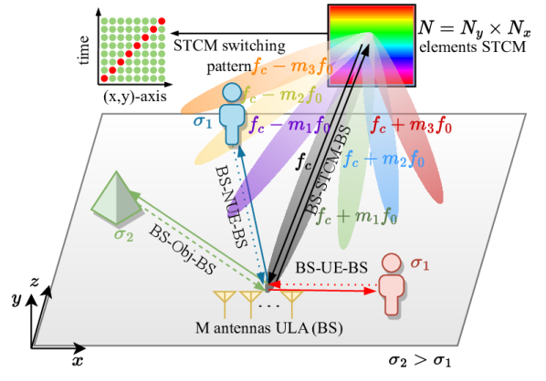
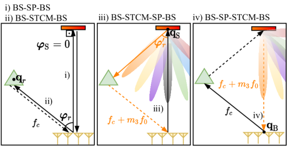
We investigate a scenario containing $K$ UEs, $\bar{K}$ NUEs, and $O$ Objs. The set of environment SPs is defined as $\mathcal{R}=\{{\rm UE}_{1},\dots,{\rm UE}_{K},{\rm NUE}_{1},\dots,{\rm NUE}_{\tilde{K}},{\rm Obj}_{1},\dots,{\rm Obj}_{O}\}$ , and $|\mathcal{R}|=(K+\tilde{K}+O)$. Fig. 1 presents the interaction of the elements in DL STCM-based M-MIMO pilot transmission. We remark that BS and STCM share the same normal, i.e. are disposed with the horizontal centers’ aligned to the origin. Upon transmission, the signals reflect in every SP and in the STCM and are received back at the BS, characterizing the single-bounce (SB) components: c1) BS-STCM-BS and c2) BS-SP-BS, as presented in Fig 1b. Moreover, the signals are subject to double-bouncing paths, i.e., c3) BS-STCM-SP-BS and c4) BS-SP-STCM-BS, which are, respectively, replicas of the transmitted signal reflected from the STCM towards the SP, and from the SP towards the STCM, and both reflected back to the BS, exemplary illustrated in Fig. 1b. The received echo signal in the $m$-th harmonic component ${\bf Y}^{\rm echo}_{m}\in\mathbb{C}^{M\times{S}}$ is formally described as:

$$\begin{split}&{\bf Y}^{\rm echo}_{m}\triangleq\bigg{(}\underbrace{\bar{\beta}_{{\rm S}}\eta_{m}(\boldsymbol{\varphi}_{{\rm S}},\boldsymbol{\varphi}_{{\rm S}}){{\bf a}_{\rm B}}(\boldsymbol{\varphi}_{{\rm S}}){{\bf a}^{\top}_{\rm B}}(\boldsymbol{\varphi}_{{\rm S}})d_{{m}}({\tau_{\rm S}})}_{\text{{\it c1)} BS-STCM-BS}}\\ &\>+\sum\limits_{r\in\mathcal{R}}\underbrace{\bar{\beta}_{r}{{\bf a}_{\rm B}}(\boldsymbol{\varphi}_{r}){{\bf a}^{\top}_{\rm B}}(\boldsymbol{\varphi}_{r})d_{{m}}({\tau_{r}})}_{\text{{\it c2)} BS-SP-BS}}\\ &\>+\sum\limits_{r\in\mathcal{R}}\underbrace{\bar{\bar{\beta}}_{r}\eta_{m}(\boldsymbol{\varphi}_{r}^{\prime},\boldsymbol{\varphi}_{{\rm S}}){{\bf a}_{\rm B}}(\boldsymbol{\varphi}_{r}){{\bf a}^{\top}_{\rm B}}(\boldsymbol{\varphi}_{{\rm S}})d_{{m}}({\tau}_{r})}_{\text{{\it c3)} BS-STCM-SP-BS}}\\ &\>+\sum\limits_{r\in\mathcal{R}}\underbrace{\bar{\bar{\beta}}_{r}\eta_{m}(\boldsymbol{\varphi}_{\rm S},\boldsymbol{\varphi}_{r}^{\prime}){{\bf a}_{\rm B}}(\boldsymbol{\varphi}_{{\rm S}}){{\bf a}^{\top}_{\rm B}}(\boldsymbol{\varphi}_{r})d_{{m}}({\tau}_{r})}_{\text{{\it c4)} BS-SP-STCM-BS}}\bigg{)}{\bf X}+{\bf N}_{m},\end{split}$$ (5)

where the scalars $\{\bar{\beta}_{r},\bar{\bar{\beta}}_{r}\}\in\mathbb{C}^{+}$ encompasses the path gain between the $r$-th SP and the BS in SB and double-bounce (DB), respectively. $\boldsymbol{\varphi}_{r}$, $\boldsymbol{\varphi}_{r}^{\prime}$, and $\boldsymbol{\varphi}_{{\rm S}}$ are the BS-SP, STCM-SP, and BS-STCM angles, respectively, ${{\bf a}_{\rm B}}(\boldsymbol{\varphi}_{r})\in\mathbb{C}^{M\times 1}$ [16, Eq. (6)], is the array response vector (RV) at the BS defined by the wavenumber ${\bf k}$ and antenna elements positions matrix ${\bf Q}_{\rm B}=[\mathbf{q}_{0},\mathbf{q}_{1},\dots\mathbf{q}_{M}]\in\mathbb{R}^{M\times 3}$ w.r.t. $\boldsymbol{\varphi}$,

$${\bf a}_{\rm B}(\boldsymbol{\varphi})={\rm exp}\big{(}j\mathbf{Q}_{\rm B}\mathbf{k}_{\lambda_{c}}(\boldsymbol{\varphi})\big{)},$$ (6)

$d_{{m}}(\tau)\triangleq{\rm exp}(-j2\pi\tau mf_{0})$ is the Doppler phase shift dependent on the SPspositions ${\bf q}_{r}$ and relative velocity in local coordinates ${\bf v}\in\mathbb{C}^{3\times 1}$, i.e. $\tau=2\frac{|{\bf q}_{\rm B}-{\bf q}_{r}|^{\top}}{\|{\bf q}_{\rm B}-{\bf q}_{r}\|^{2}\lambda}{\bf v}$ [17]. Throughout this work, we have adopted fully static scenarios. Hence, ${\tau_{r}=\tau_{\rm S}}=0$, so $d_{{m}}(\tau)=1$. ${\bf X}={\bf w}{\bf s}\,\in\mathbb{C}^{M\times S}$ denotes the $S$ transmitted symbols vector ${\bf s}\in\mathbb{C}^{1\times S}$ using a precoding vector ${\bf w}\in\mathbb{C}^{M\times 1}$, encompassing both directivity and transmit power, ${\bf N}_{m}\sim\mathcal{CN}({\bf 0},\sigma_{n}^{2}{\bf I}_{M})$ is the additive white Gaussian noise (AWGN) at the BS and $\eta_{m}(\boldsymbol{\varphi}_{D},\boldsymbol{\varphi}_{A})\in\mathbb{C}$, Eq. (3), denotes the STCM steered RV w.r.t. AoA $\boldsymbol{\varphi}_{\rm A}$ and AoD $\boldsymbol{\varphi}_{\rm D}$ at $m$-th harmonic. Finally, the SB and DB path gains are calculated, respectively, as

$$\bar{\beta}_{r}=G(\bar{d}_{r})\exp\left(-j2\pi\frac{\bar{d}_{r}}{c}\right)\sigma_{r}\nu,$$ (7a)

$$\bar{\bar{\beta}}_{r}=G(\bar{\bar{d}}_{r})\exp\left(-j2\pi\frac{\bar{\bar{{d}}}_{r}}{c}\right)\sigma_{r}\nu,$$ (7b)

$$G(d)=\frac{\sqrt{E_{s}}\lambda}{4\pi d^{\iota}}$$ (7c)

for $d>0$, and where $\bar{d}_{r}=2d_{r}$ and $\bar{\bar{d}}_{r}=d_{\rm S}+d_{r}+{d_{r^{\prime}}}$, with $d_{r}=\|{\bf q}_{\rm B}-{\bf q}_{r}\|$, $d_{\rm S}=\|{\bf q}_{\rm B}-{\bf q}_{\rm S}\|$, and $d_{r^{\prime}}=\|{\bf q}_{\rm S}-{\bf q}_{r}\|$ being the BS-SP, BS-STCM, and STCM-SP Euclidean distances, respectively, with ${\bf q}_{\rm B}$, ${\bf q}_{\rm S}$, and ${\bf q}_{r}$ being the coordinates of the center of the BS antennas, center of the STCM elements, and $r$-th SP coordinate, respectively. $\iota$ encompasses the square root path-loss exponent $\bar{d}_{r}/c$, and $\bar{\bar{d}}_{r}/c$ are the delays of SB and DB echo signals due to different time-of-arrival (ToA), $E_{s}$ is the symbol energy. The parameter $\sigma^{2}_{r}{\in\mathbb{R}^{+}}$ represents the RCS of the $r$-th SP which models both the attenuation and phase shifts on backscattered signals and is dependent on object properties, incident angle, carrier frequency, and its effective reflection area [18]; and $\nu\sim\mathcal{CN}(0,\sigma^{2}_{\nu})$ models multipath components related to specular reflection, diffraction, refraction, and creeping wave phenomenons [19] around SPs.

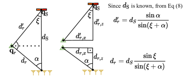
The set BS-SP-STCM form a triangle in space, Fig. 1c, with its’ side lengths as $d_{r}$ (BS-SP), $d_{\rm S}$ (BS-STCM), and $d_{r}^{\prime}$ (STCM-SP), which are a priori unknown. However, it is feasible to assume a fixed position for the STCM, since the control of such a device is done by a backhaul link to the BS; as a result, one can derive a trigonometric relationship between these three spatial points. Assuming a two-dimensional (2D) plane defined by the localization of BS, SP, and STCM sharing the same vertical $y$-axis height, simplifying $\boldsymbol{\varphi}_{r}=\alpha$ and $\boldsymbol{\varphi}_{r}^{\prime}=\xi$, regarding only the azimuth angles $(\theta_{r}=0\ \forall\ r)$, the trigonometric relationship simplifies:

$$\frac{d_{\rm S}}{\sin\zeta}=\frac{d_{r}}{\sin{\xi}}=\frac{d_{r}^{\prime}}{\sin{\alpha}},$$ (8)

where $\zeta=\pi-{\alpha}-{\xi}$, giving us enough information to localize an SP, avoiding to calculate the distance from a SP by the path gain. Finally, one can calculate $d_{r}=d_{S}\frac{\sin\xi}{\sin(\alpha+{\xi})}$, with the $r$-th SP coordinates ${\bf q}_{r}={[q_{r,x},q_{r,y},q_{r,z}]}$ as $q_{r,x}=q_{{\rm B},x}+d_{r}\sin\alpha$ and $q_{r,z}=q_{{\rm B},z}+d_{r}\cos\alpha$, while $q_{r,z}=0$.

III Space-frequency sensing with STCM

The basic framework for recovering an SP localization in the proposed STCM-aided ISAC system relies on using trigonometrical properties of the multipath bouncing, accessing the potential of recovering them at the BS upon receiving the echo signal. When the BS can recover the angles between itself and the SP and STCM-SP, it provides a robust estimation method regarding the stochastic characteristics of the path. Classical triangulation relies on synchronization and sensing by multiple BSs, which is demanding both computationally and in terms of energy consumption. Alternatively, the STCM acts like a semi-passive artificial signal emitter, and its’ intrinsic properties are useful for estimating the angle between this device and potential SPs. Thus, the processing is done centralized at the BS by estimating the SPs’ AoA and the angle between the SPs and the STCM. For the sake of simplicity, throughout this work we consider: a) 2-D scenarios, as introduced in Sec. II, and b) non-mobility, static scenarios, hence $\{\bar{\tau},\bar{\bar{\tau}}\}=0$. Fig. 1c depicts a comprehensive diagram justifying the trigonometric calculation in Eq.(8).

The estimation of angle $\alpha$ is immediate by any classic estimator, such as MUSIC, ESPRIT, MVDR, and others, while estimating $\xi$ relies upon the relationship between the received power gain of harmonics frequencies generated by STCM. Knowing the distance $d_{\rm S}$, we can estimate $d_{r}$, hence retrieving the SP location with high precision, using the trigonometric relation in Eq. (8), Fig. 1c.

Assumptions. The following assumptions are adopted. The components c1), c2), and c3)-c4) in Eq. (5) have different ToA at the BS array, hence the signal processing can be carried out separately. We divide the processing framework by using c2) to estimate $\alpha$ and c3)-c4) to estimate $\xi$ by deploying the relationship between the harmonics power level generated at the STCM and considering far-field condition, in same way as adopted in [11]. In other words, different AoD and AoA at the STCM generate a unique vector of power gains of components observed at the BS, which are a basis of inference for this angle. The latter components which experience DB, can not be dissociated since they have the same ToA due to their traveled distance being the same. Hence, we estimate angle $\xi$ by deploying harmonic signals generated at the STCM arriving with the different power gains.

III-A Localization Problem

Under these considerations, to formulate and assess the SPlocalization the capability of such a setup, we rely on the information theory Cramér-Rao bound (CRB) computations. We also assume the position and orientation of the STCM are known in advance. Indeed, such an assumption is reasonable since the estimation can be done in a prior step where one might use time-orthogonal STCM sequences to cancel any other interference. Besides, the BS knows the STCM position since its control relies on a backhaul link; hence, such prior information is feasible.

Cramér-Rao Bound: The CRB gives us the lower bound of the covariance among unbiased estimators on unknown deterministic and/or stochastic parameters. Estimators achieving this lower bound are called unbiased and fully efficient estimators [20]. Such a property can be found, e.g., in the maximum likelihood estimator which is unbiased and efficient in the context of linear models, and for non-linear models, this weakens to asymptotically unbiased and efficient. To estimate the localization of an SP one can estimate the sufficient information $\alpha$ and $\xi$ angles, Fig. 1c, characterizing a multivariate case, where the quality of estimation of both angles subject to the path gains. Relying on the capacity of processing separately the SB and DB components, we split the respective parameter sets to be estimated as:

$$\begin{split}\boldsymbol{\Psi}^{\rm SB}=[\alpha,\tilde{\bar{\boldsymbol{\beta}}}]=[\alpha_{1},\dots,\alpha_{|\mathcal{R}|},{\rm Re}\{\bar{\beta}_{1}\},{\rm Im}\{\bar{\beta}_{1}\},\\ \dots,{\rm Re}\{\bar{\beta}_{|\mathcal{R}|}\},{\rm Im}\{\bar{\beta}_{|\mathcal{R}|}\}]\in\mathbb{R}^{1\times 3|\mathcal{R}|},\end{split}$$ (9)

and

$$\begin{split}\boldsymbol{\Psi}^{\rm DB}=[\xi,\tilde{\bar{\bar{\boldsymbol{\beta}}}}]=[\xi_{1},\dots,\xi_{|\mathcal{R}|},{\rm Re}\{\bar{\bar{\beta}}_{1}\},{\rm Im}\{\bar{\bar{\beta}}_{1}\},\\ \dots,{\rm Re}\{\bar{\bar{\beta}}_{|\mathcal{R}|}\},{\rm Im}\{\bar{\bar{{\beta}}}_{|\mathcal{R}|}\}]\in\mathbb{R}^{1\times 3|\mathcal{R}|},\end{split}$$ (10)

which are the deterministic parameters ($\alpha,\xi$) and mixed deterministic-stochastic $(\bar{\beta},\bar{\bar{\beta}})$ organized as $\tilde{\bar{{\boldsymbol{\beta}}}}=[{\rm Re}\{\bar{\boldsymbol{\beta}}\},{\rm Im}\{\bar{\boldsymbol{\beta}}\}]$ and $\tilde{\bar{\bar{\boldsymbol{\beta}}}}=[{\rm Re}\{\bar{\bar{\boldsymbol{\beta}}}\},{\rm Im}\{\bar{\bar{\boldsymbol{\beta}}}\}]$ unknown variables.

Let $\mathcal{M}=\{-m_{f},-(m_{f}-1),\dots,m_{f}\}$ be the set of analyzed harmonics, including 0 (central frequency), and $|\mathcal{M}|$ the cardinality of the set. Before proceeding, we rearrange the echo signal (5) into the SB and DB parts while stacking the signals in a vector. Let $\hat{\bf n}^{\rm SB}={\rm vec}({\bf N}_{0})\in\mathbb{C}^{\cdot M\cdot S\times 1}$ and $\hat{\bf n}^{\rm DB}=[{\rm vec}({\bf N}_{-m_{f}}),\dots,{\rm vec}({\bf N}_{m_{f}})]^{\top}\in\mathbb{C}^{|\mathcal{M}|\cdot M\cdot S\times 1}$, where vec$(\cdot)$ refers to the vectorization of the matrix, be the vectorized noise and let

$${\bf H}^{\rm SB}({\bf q}_{r})={\rm vec}({{\bf a}_{\rm B}}(\boldsymbol{\varphi}_{r}){{\bf a}^{\top}_{\rm B}}(\boldsymbol{\varphi}_{r}){\bf X})^{{\top}}\in\mathbb{C}^{M\cdot S\times 1}$$

be the deterministic part of the SB signal, i.e. component c2). Then, the SB signal is given as

$$\hat{\bf y}^{\rm SB}=\sum\limits_{r\in\mathcal{R}}\hat{\bf u}^{\rm SB}({\bf q}_{r})+\hat{\bf n}^{\rm SB}$$ (11)

where $\hat{\bf u}^{\rm SB}({\bf q}_{r})=\bar{\beta}_{r}{\bf H}^{\rm SB}({\bf q}_{r})$. Similarly, for the DB signal let us define ${\boldsymbol{\eta}}(\boldsymbol{\varphi},\boldsymbol{\varphi}^{\prime})=[{\bf\eta}_{-m_{f}}(\boldsymbol{\varphi},\boldsymbol{\varphi}^{\prime}),\dots,{\bf\eta}_{m_{f}}(\boldsymbol{\varphi},\boldsymbol{\varphi}^{\prime})]^{\top}$, and let

$$\begin{split}&{\bf H}^{\rm DB}({\bf q}_{r})={\boldsymbol{\eta}}(\boldsymbol{\varphi}_{r}^{\prime},\boldsymbol{\varphi}_{\rm S})\otimes{\rm vec}({{\bf a}_{\rm B}}(\boldsymbol{\varphi}_{r}){{\bf a}^{\top}_{\rm B}}(\boldsymbol{\varphi}_{\rm S}){\bf X})^{{\top}}\\ &\quad+{\boldsymbol{\eta}}(\boldsymbol{\varphi}_{\rm S},\boldsymbol{\varphi}_{r}^{\prime})\otimes{\rm vec}({{\bf a}_{\rm B}}(\boldsymbol{\varphi}_{\rm S}){{\bf a}^{\top}_{\rm B}}(\boldsymbol{\varphi}_{r}){\bf X})^{{\top}}\in\mathbb{C}^{|\mathcal{M}|\cdot M\cdot S\times 1}.\end{split}$$

where $\otimes$ denotes the Kronecker product. The DB signal is then

$$\hat{\bf y}^{\rm DB}=\sum\limits_{r\in\mathcal{R}}\hat{\bf u}^{\rm DB}({\bf q}_{r})+\hat{\bf n}^{\rm DB}$$ (12)

where $\hat{\bf u}^{\rm DB}({\bf q}_{r})=\bar{\bar{\beta}}_{r}{\bf H}^{\rm DB}({\bf q}_{r})$.

We use this arrangement to calculate the mutual information matrices of SB and DB paths. In the present case of AWGN, the Fisher information matrix (FIM) is computed as

$$\begin{split}\hat{\bf{F}}_{i,j}=\frac{2}{\sigma_{n}^{2}}{\rm Re}\left\{\frac{\partial}{\partial{\Psi}_{i}}\hat{\bf u}\frac{\partial}{\partial{\Psi}_{j}}\hat{\bf u}\right\}.\end{split}$$ (13)

Moreover, to simplify the notation, we use $\hat{\bf F}_{{\Psi}_{i}{\Psi}_{j}}$ to refer to the general formula of Eq. (13). In the following, we calculate both FIM matrices related to the SB and DB paths.

SB path CRB: We consider that the BS is capable of totally nullifying the echo signal component c1) and process individually the component c2) as the SB path, as discussed previously. Hence, three variables affect this signal, as depicted before. We can evaluate the FIMmatrix by arranging the variables contained in $\boldsymbol{\Psi}^{\rm SB}$ applying Eq. (13). For illustration purposes, let’s consider a single SP scenario, where the FIM has the following form

$${\bf F}^{\rm SB}=\left[\begin{matrix}\hat{\bf F}_{\alpha\alpha}&\hat{\bf F}_{\alpha\tilde{\bar{\beta}}}\\ \hat{\bf F}_{\alpha\tilde{\bar{\beta}}}^{\top}&\hat{\bf F}_{\tilde{\bar{\beta}}\tilde{\bar{\beta}}}\end{matrix}\right].$$ (14)

We begin by computing the partial derivatives as $\frac{\partial}{\partial\alpha}\hat{\bf u}^{\rm SB}=\bar{\beta}\dot{\bf A}(\alpha){\bf X}$ and $\frac{\partial}{\partial\tilde{\bar{\beta}}}\hat{\bf u}^{\rm SB}=[1,j]\otimes{\bf AX}$, where ${\bf A}(\alpha)={{\bf a}_{\rm B}}(\alpha){{\bf a}^{\top}_{\rm B}}(\alpha)$, $\dot{\bf A}(\alpha)=\frac{\partial}{\partial\alpha}{\bf A}(\alpha)$. Taking the empirical sample covariance matrix over $S$ transmitted symbols as:

$${\bf R}_{\bf x}=\frac{1}{S-1}\sum_{s=1}^{S}{\bf x}[s]{\bf x}^{\rm H}[s],$$ (15)

we evaluate

$$\hat{\bf F}_{\alpha\alpha}= \frac{2S{|\bar{\beta}|}^{2}}{\sigma^{2}_{n}}{\rm tr}(\dot{\bf A}(\alpha){\bf R}_{\bf x}\dot{\bf A}^{\rm H}(\alpha)),$$ (16a)

$$\hat{\bf F}_{\alpha\tilde{\bar{\beta}}}= \frac{2S}{\sigma^{2}_{n}}{\rm Re}\{{\bar{\beta}}^{*}{\rm tr}({\bf A}(\alpha){\bf R}_{\bf x}\dot{\bf A}^{\rm H}(\alpha))[1,j]\},$$ (16b)

$$\hat{\bf F}_{\tilde{\bar{\beta}}\tilde{\bar{\beta}}}= \frac{2S}{\sigma^{2}_{n}}{\rm tr}({\bf A}(\alpha){\bf R}_{\bf x}{\bf A}^{\rm H}(\alpha)){\bf I}_{2}$$ (16c)

Finally, we obtain the CRB of estimating angle $\alpha$ corresponds to the first element of ${{\bf F}^{\rm SB}}^{-1}$ as:

$$\begin{split}\scriptsize[{{\bf F}^{\rm SB}}^{-1}]_{1,1}=\frac{\sigma^{2}_{n}}{2S{|\bar{\beta}|}^{2}\bigg{(}{\rm tr}(\dot{\bf A}{\bf R}_{\bf x}\dot{\bf A}^{\rm H})-\frac{{|{\rm tr}({\bf A}{\bf R}_{\bf x}\dot{\bf A}^{\rm H})|}^{2}}{{\rm tr}({\bf A}{\bf R}_{\bf x}{\bf A}^{\rm H})}\bigg{)}}.\end{split}$$ (17)

DB path CRB: analogously, we can calculate the CRB for the DBpaths by arranging the FIM with the elements contained in the set $\boldsymbol{\Psi}^{\rm DB}$ and processing with the re-arranged signal $\hat{\bf y}^{\rm DB}$. We can straightforwardly infer the following matrix for single SP target CRB calculation:

$${\bf F}^{\rm DB}=\left[\begin{matrix}\hat{\bf F}_{\xi\xi}&\hat{\bf F}_{\xi\tilde{\bar{\bar{\beta}}}}\\ \hat{\bf F}_{\xi\tilde{\bar{\bar{\beta}}}}^{\top}&\hat{\bf F}_{\tilde{\bar{\bar{\beta}}}\tilde{\bar{\bar{\beta}}}}\end{matrix}\right],$$ (18)

where

$$\frac{\partial}{\partial\xi}\hat{\bf u}^{\rm DB}_{m}=\bar{\bar{\beta}}{\rm vec}\big{(}\dot{\eta}_{m}(\xi,0){\bf A}(\alpha,0)+\dot{\eta}_{m}(0,\xi){\bf A}(0,\alpha)\big{)}{\bf X},$$

and

$$\frac{\partial}{\partial\bar{\bar{\beta}}}\hat{\bf u}=[1,j]\otimes{\rm vec}(\eta_{m}{\bf A}(\alpha,0)+\eta_{m}{\bf A}(0,\alpha)){\bf X}$$

for the frequency-domain far-field pattern of the $m$-th harmonic $\eta_{m}$, described in Eq. (3); $\eta_{m}(0,\xi)$ and $\eta_{m}(\xi,0)$ and its derivatives assume equal complex value in both phase and magnitude due to specular reflection by the STCM. In this context, ${\bf A}(\theta_{i},\theta_{j})={{\bf a}_{\rm B}}(\phi_{i}){{\bf a}^{\top}_{\rm B}}(\phi_{j})={\bf A}^{\top}(\phi_{j},\phi_{i})\triangleq{\bf A}\ \forall\ i,j$.

We can simplify the above equations to obtain $\frac{\partial}{\partial\xi}\hat{\bf u}^{\rm DB}_{m}=\bar{\bar{\beta}}{\rm vec}\big{(}\dot{\eta}_{m}({\bf A}+{\bf A}^{\top}){\bf X}\big{)}=\bar{\bar{\beta}}{\rm vec}\big{(}\dot{\eta}_{m}{\bf B}{\bf X}\big{)}$ and $\frac{\partial}{\partial\bar{\bar{\beta}}}\hat{\bf u}^{\rm DB}_{m}=[1,j]\otimes{\rm vec}(\eta_{m}{\bf BX})$. Hence, supporting in Eq. (13) we can evaluate a closed-form expression as in the SB case. Consider $\boldsymbol{\eta}=[\eta_{-mf},\eta_{-(mf-1)},\dots,\eta_{mf}]\in\mathbb{C}^{|\mathcal{M}|\times 1}$ and $\dot{\boldsymbol{\eta}}=[\dot{\eta}_{-mf},\dot{\eta}_{-(mf-1)},\dots,\dot{\eta}_{mf}]\in\mathbb{C}^{|\mathcal{M}|\times 1}$ and let:

$$\hat{\bf F}_{\xi\xi} =\frac{2S{|\bar{\bar{\beta}}|}^{2}}{\sigma^{2}_{n}}(\dot{\boldsymbol{\eta}}^{\rm H}\dot{\boldsymbol{\eta}}){\rm tr}({\bf B}{\bf R}_{\bf x}{\bf B}^{\rm H}),$$ (19a)

$$\hat{\bf F}_{\xi\tilde{\bar{\bar{\beta}}}} =\frac{2S}{\sigma^{2}_{n}}{\rm Re}\{(\dot{\boldsymbol{\eta}}^{\rm H}{\boldsymbol{\eta}}){{\bar{\bar{\beta}}}}^{*}{\rm tr}({\bf B}{\bf R}_{\bf x}{\bf B}^{\rm H})[1,j]\},$$ (19b)

$$\hat{\bf F}_{\tilde{\bar{\bar{\beta}}}\tilde{\bar{\bar{\beta}}}} =\frac{2S}{\sigma^{2}_{n}}({\boldsymbol{\eta}}^{\rm H}{\boldsymbol{\eta}}){\rm tr}({\bf B}{\bf R}_{\bf x}{\bf B}^{\rm H}){\bf I}_{2}.$$ (19c)

Then, the closed-form expression $[{{\bf F}^{\rm DB}}^{-1}]_{1,1}$ is defined as:

$$\begin{split}[{{\bf F}^{\rm DB}}^{-1}]_{1,1}=\frac{\sigma^{2}_{n}}{2S{|\bar{\bar{\beta}}|}^{2}{\rm tr}({\bf B}{\bf R}_{\bf x}{\bf B}^{\rm H})-\bigg{(}\dot{\boldsymbol{\eta}}^{\rm H}\dot{\boldsymbol{\eta}}-\frac{(\dot{\boldsymbol{\eta}}^{\rm H}{\boldsymbol{\eta}})^{2}}{{\boldsymbol{\eta}}^{\rm H}{\boldsymbol{\eta}}}\bigg{)}}.\end{split}$$ (20)

It is straightforward to infer that the more harmonics being employed the higher the sensing capabilities, presenting a trade-off between complexity and performance. The parameter of design then becomes both $a_{pq}^{m}$, Eq. (4), and the transmit signals covariance matrix ${\bf R}_{\bf x}$. Optimizing the localization capabilities of the system means minimizing the closed-form expressions in eqs. (17) and (20), respectively.

III-A1 CRB on Localization

To derive the CRB on the positions of the SPs in Euclidean coordinates we begin by computing the equivalent Fisher information of the angle parameters. For the SB signal

$$\bf{F}^{\rm EFIM}_{\alpha\alpha}=\hat{\bf{F}}_{\alpha\alpha}-\hat{\bf{F}}_{\alpha\tilde{\bar{\beta}}}\hat{\bf{F}}^{-1}_{\tilde{\bar{\beta}}\tilde{\bar{\beta}}}\hat{\bf{F}}_{\alpha\tilde{\bar{\beta}}}^{\top},$$ (21)

and for the double bounce signals

$$\bf{F}^{\rm EFIM}_{\xi\xi}=\hat{\bf{F}}_{\xi\xi}-\hat{\bf{F}}_{\xi\tilde{\bar{\bar{\beta}}}}\hat{\bf{F}}^{-1}_{\tilde{\bar{\bar{\beta}}}\tilde{\bar{\bar{\beta}}}}\hat{\bf{F}}_{\xi\tilde{\bar{\bar{\beta}}}}^{\top}.$$ (22)

Then, assuming independence between the estimation of the $\alpha$ and $\xi$ angles, we define the Fisher information matrix for the position-relevant information as

$$\bf{F}^{\rm EFIM}=\begin{pmatrix}\bf{F}^{\rm EFIM}_{\alpha\alpha}&0\\ 0&\bf{F}^{\rm EFIM}_{\xi\xi}\end{pmatrix}.$$ (23)

We define the Jacobian of the mapping from the angles to the position ${\bf q}=(x,{0},z)$ as

$$\bf{T}=\begin{pmatrix}\frac{\partial\alpha}{\partial x}&\frac{\partial\alpha}{\partial z}\\ \frac{\partial\xi}{\partial x}&\frac{\partial\xi}{\partial z}\end{pmatrix}.$$ (24)

One can rewrite the angles as a the function of their position in local coordinates, Fig. 1b, 1c, as:

$$\alpha=\arctan\frac{q_{r,x}-q_{{\rm B},x}}{q_{r,z}-q_{{\rm B},z}}\qquad\text{and}\qquad\xi=\arctan\frac{q_{r,x}-q_{{\rm S},x}}{q_{r,z}-q_{{\rm S},z}}$$

Let coordinates $q_{x}$ and $q_{z}$ denote the point ${\bf q}(x,0,z)={(q_{x},0,q_{z})}$ in local coordinates, we can find the elements in Eq. (24) as

$$\frac{\partial\alpha}{\partial x}= \frac{q_{{\rm B},z}-q_{z}}{(q_{x}-q_{{\rm B},x})^{2}+(q_{z}-q_{{\rm B},z})^{2}},$$ (25a)

$$\frac{\partial\alpha}{\partial z}= \frac{q_{x}-q_{{\rm B},x}}{(q_{x}-q_{{\rm B},x})^{2}+(q_{z}-q_{{\rm B},z})^{2}},$$ (25b)

$$\frac{\partial\xi}{\partial x}= \frac{q_{{\rm S},z}-q_{z}}{(q_{x}-q_{{\rm S},x})^{2}+(q_{z}-q_{{\rm S},z})^{2}},$$ (25c)

$$\frac{\partial\xi}{\partial z}= \frac{q_{x}-q_{{\rm S},x}}{(q_{x}-q_{{\rm S},x})^{2}+(q_{z}-q_{{\rm S},z})^{2}}.$$ (25d)

Then the single SP Fisher information on the position ${\bf q}={(q_{x},0,q_{z})}$ is

$$\bf{F}(\bf{q})={\bf T}^{{\top}}{{\bf F}^{\rm EFIM}}{\bf T}$$ (26)

and the CRB on the position is ${\bf F}^{-1}({\bf q})$. We define the position error bound (PEB) as [21]:

$${\rm PEB}({\bf q})=\sqrt{{\rm Tr}({\bf F}^{-1}({\bf q}))}.$$ (27)

Remark: Multiple SP position error bound (PEB) can be calculated via software by expanding the matrix ${\bf F}^{\rm EFIM}$ to multiple values of $\alpha$ and $\xi$, but obtaining closed form solutions is not practical in multiple SP scenarios.

III-B Detection and Classification

The detection problem relates not to estimating the localization of the SP but rather to detecting its presence. This can be formulated as a hypothesis testing problem where the null hypothesis is the presence of no target and the alternate hypothesis is the presence of a target. The task of classification relates to determining which kind of SP a detected target is and can also be formulated as a hypothesis-testing problem. In the following, we present the signal model in a general setting which can straightforwardly be used for both SB and DB signals (see eqs. (11) and (12)) and construct the competing hypotheses.

The received echo signal from an SP at position ${\bf q}_{r}$ under hypothesis $\mathcal{H}_{i}$ can be expressed as

$${\bf Y}=\beta_{i}{\bf H}({\bf q}_{r})+\bf{N}$$ (28)

where ${\bf N}\sim\mathcal{CN}(0,\sigma^{2}_{n}{\bf I}_{M})$ is AWGN, $M$ is the dimension of the received signal, and the path gain

$$\beta_{i}=G(d)\sigma_{i}\nu$$ (29)

for $i=0,1,2$, where $\nu\sim\mathcal{CN}(0,\sigma^{2}_{\nu})$ is the fading coefficient, and $\sigma_{i}$ is the square root of the radar cross section (RCS) with $\sigma_{0}=0$, i.e. absence of SP, $\sigma_{1}$ refers to a NUE or UE SP type, and $\sigma_{2}$ refers to an object with polished surface (Obj) SP type, with RCS $\sigma_{1}<\sigma_{2}$. Then, the amplitude $|\nu|$ is Rayleigh distributed with scale parameter $\sigma_{\nu}$. We know that $|\beta_{i}|$ follows a Rayleigh distribution $R(\cdot;\varsigma)$ with scale parameter $\varsigma(\cdot)>0$:

$${\varsigma}(\sigma_{i})=G(d)\sigma_{i}\sigma_{\nu}{\left(\frac{\pi}{2}\right)^{-\frac{1}{2}}}.$$ (30)

III-B1 Detection Analysis

Herein, we will assume that the position $\boldsymbol{q}{{}_{r}}$ is known, which for detection can make practical sense: we sweep through each location $\boldsymbol{q}{{}_{r}}$ and make the detection decision. Under such an assumption, the maximum likelihood estimator of the channel coefficient can be written as:

$$\hat{\beta}({\bf{Y}})=\frac{{\bf H}({\bf q}{{}_{r}})^{H}\bf{{Y}}}{\|{\bf H}({\bf q}{{}_{r}})\|^{2}}$$ (31)

with distribution $\hat{\beta}\sim\mathcal{CN}\big{(}\beta_{i},\,\frac{\sigma^{2}_{{n}}}{\|\boldsymbol{H}(\boldsymbol{q{{}_{r}}})\|^{2}}\big{)}$. Hence, the statistic $\tilde{\gamma}\triangleq\frac{2\|\boldsymbol{H}(\boldsymbol{q{{}_{r}}})\|^{2}}{\sigma^{2}_{{n}}}|\hat{\beta}|^{2}$ follows a non-central $\chi^{2}$ distribution with $2$ degrees of freedom and non-centrality parameter $\mu_{\tilde{\gamma}}\triangleq\frac{2\|\boldsymbol{H}(\boldsymbol{q{{}_{r}}})\|^{2}}{\sigma^{2}_{{n}}}|\beta_{i}|^{2}$. Given $\beta_{i}$ and a detection threshold $\gamma_{\text{th}}$, the conditional detection probability is given by

$$p_{{}_{\text{D}}}(\beta_{i})=f_{\tilde{\gamma}}(\tilde{\gamma}>\gamma_{\text{th}}|\beta_{i})=Q_{1}\big{(}\sqrt{\mu_{\tilde{\gamma}}},\sqrt{\gamma_{\text{th}}}\big{)}$$ (32)

where $Q_{1}(\cdot,\cdot)$ is the Marcum Q-function. The false alarm probability is related to the detection threshold $\gamma_{\text{th}}$ by

$$p_{{}_{\text{FA}}}=f_{\tilde{\gamma}}(\tilde{\gamma}>\gamma_{\text{th}}|\beta_{i}=0)=e^{-\frac{\gamma_{\text{th}}}{2}}$$ (33)

such that $\gamma_{\text{th}}=-2\,{\ln}\,p_{{}_{\text{FA}}}$ for a specified false alarm probability [22]. In the above expression, we condition on the realization of the fading $\beta_{i}$; however, we may also be interested in the marginal distribution which can be expressed as [23]

$$p_{{}_{\text{D}}}=\int f_{\tilde{\gamma}}(\tilde{\gamma}>\gamma_{\text{th}}|\beta_{i})f_{\beta_{i}}(\beta_{i})d\beta_{i}.$$ (34)

Solving the integral and simplifying the terms, (34) can be expressed as:

$$p_{\textsc{d}}=\exp\left(-\frac{\gamma_{\rm th}\sigma_{n}^{2}}{4{\|{\bf H}({\bf q})\|^{2}\ {\varsigma}(\sigma_{i})^{2}+2\sigma_{n}^{2}}}\right).$$ (35)

Hence, the probability of detection of an SP is dependent on the probability of a false alarm, which can be set or experimentally approximated, the noise level, the BS-SP array RV of the echo signal, including the transmitted power and symbols. Finally, the SP-BS distance and the RCS, both contained in ${\varsigma}(\sigma_{i})$, determine whether the BS is capable of detecting a scatter target.

III-C Classification Modelling in STCM Sensing

Given an observation ${\bf{Y}}(\beta_{i})$, we derive the posterior probabilities for the three hypotheses. Using Bayes’ formula, we have

$$\text{Pr}(\mathcal{H}_{i}|{{\bf Y}}(\beta_{i}))=\frac{\text{Pr}({{\bf Y}}(\beta_{i})|\mathcal{H}_{i})\text{Pr}(\mathcal{H}_{i})}{\displaystyle\sum_{i=0}^{2}\text{Pr}({{\bf Y}}(\beta_{i})|\mathcal{H}_{i})\text{Pr}(\mathcal{H}_{i})}.$$ (36)

Without prior knowledge of the hypotheses, we have $\text{Pr}(\mathcal{H}_{0})=\text{Pr}(\mathcal{H}_{1})=\text{Pr}(\mathcal{H}_{2})=\frac{1}{3}$ in the detection/classification scenario of Fig. 1a, where the hypotheses $\mathcal{H}_{1}$ and $\mathcal{H}_{2}$ refer to the type of SP, being $1$ the NUE, and $2$ the Obj; besides, hypothesis $\mathcal{H}_{0}$ refers to high instantaneous noise level but there are no SP at the position analyzed, indicating a false alarm configuration. Notice that these prior probabilities can be tuneable parameters chosen depending on the application purposes. Also, given that we have detected a point, we may assume that $\text{Pr}(\mathcal{H}_{0})$ is low.

We assume that given the data ${{\bf Y}}(\beta_{i})$, an estimate of $\beta_{i}$ is computed as $\hat{\beta}=\hat{\beta}({{\bf Y}}(\beta_{i}))$. Moreover, we say that $\hat{\beta}\sim f_{\hat{\beta}}(\cdot;\beta_{i})$ follows a distribution with some density depending on the observation and thereby the realization of the channel $\beta_{i}$. The difference here compared to the setup in the detection analysis, is that we no longer assume that the position of the SP is known, and then this uncertainty on the position will also affect the uncertainty in the estimator $\beta_{i}$.

To simplify the analysis, we assume that the estimator $\hat{\beta}$ is a sufficient statistic of the data ${{\bf Y}}(\beta_{i})$ with respect to the parameter $\beta_{i}$, such that the classification problem becomes

$$\text{Pr}(\mathcal{H}_{i}|\hat{\beta})=\frac{\text{Pr}(\hat{\beta}|\mathcal{H}_{i})\text{Pr}(\mathcal{H}_{i})}{\displaystyle\sum_{i=0}^{2}\text{Pr}(\hat{\beta}|\mathcal{H}_{i})\text{Pr}(\mathcal{H}_{i})}.$$ (37)

We expand the conditional probabilities as

$$\text{Pr}(\hat{\beta}|\mathcal{H}_{i}) =\int\text{Pr}(\hat{\beta}|\beta)\text{Pr}(\beta|\mathcal{H}_{i})d\beta$$ (38)

$$=\int\text{Pr}(\hat{\beta}|\beta_{i})\text{Pr}(\beta_{i})d\beta_{i}$$ (39)

by exploiting the fact that $\hat{\beta}$ and $\mathcal{H}_{i}$ are conditionally independent given $\beta$. We remark then that $\text{Pr}(\hat{\beta}|\beta_{i})=f_{\hat{\beta}}(\hat{\beta};\beta_{i})$ and $\text{Pr}(\beta_{i})=\mathcal{CN}(\beta_{i};0,(G(d)\sigma_{i}\sigma_{\nu})^{2})$. Using the maximum a posteriori rule, we would choose the hypothesis with the highest posterior probability, i.e., we estimate the class as

$$\hat{i}=\operatorname*{arg\,\max}_{i\in\{0,1,2\}}\leavevmode\nobreak\ \leavevmode\nobreak\ \text{Pr}(\mathcal{H}_{i}|\hat{\beta})$$ (40)

and the chosen hypothesis is $\hat{\mathcal{H}}=\mathcal{H}_{\hat{i}}$. [24]

Special Case: circular covariance: In this part, we assume for simplicity that the estimator of the channel coefficient follows a circular covariance, i.e., $\hat{\beta}({\bf Y}(\beta_{i}))\sim\mathcal{CN}(\beta_{i},\sigma_{\hat{\beta}}^{2})$ for some variance parameter $\sigma_{\hat{\beta}}^{2}$. In this case, following the same arguments as in the detection analysis, the statistic $\tilde{\gamma}\triangleq\frac{2}{\sigma_{\hat{\beta}}^{2}}|\hat{\beta}|^{2}$ follows a non-central $\chi^{2}$ distribution with $2$ degrees of freedom and non-centrality parameter $\mu_{\tilde{\gamma}}\triangleq\mu_{\tilde{\gamma}}(|\beta_{i}|)\triangleq\frac{2}{\sigma_{\hat{\beta}}^{2}}|\beta_{i}|^{2}$. The density function for $\tilde{\gamma}$ is then

$$f_{\tilde{\gamma}}(\tilde{\gamma};\mu_{\tilde{\gamma}})=\frac{1}{2}I_{0}\Big{(}\sqrt{\mu_{\tilde{\gamma}}\tilde{\gamma}}\Big{)}\exp\Big{\{}-\frac{\tilde{\gamma}+\mu_{\tilde{\gamma}}}{2}\Big{\}}$$ (41)

By a variable transformation, we find the density for $|\hat{\beta}|$ as

$$f_{|\hat{\beta}|}(|\hat{\beta}|;\mu_{\tilde{\gamma}}) =\Big{|}\frac{d\tilde{\gamma}}{d|\hat{\beta}|}\Big{|}f_{\tilde{\gamma}}\Big{(}\frac{2|\hat{\beta}|^{2}}{\sigma_{\hat{\beta}}^{2}};\mu_{\tilde{\gamma}}\Big{)}$$

$$=\frac{2|\hat{\beta}|}{\sigma^{2}_{\hat{\beta}}}I_{0}\Bigg{(}\sqrt{2\mu_{\tilde{\gamma}}}\frac{|\hat{\beta}|}{\sigma_{\hat{\beta}}}\Bigg{)}\exp\Bigg{\{}-\Big{(}\frac{|\hat{\beta}|^{2}}{\sigma^{2}_{\hat{\beta}}}+\frac{\mu_{\tilde{\gamma}}}{2}\Big{)}\Bigg{\}}.$$ (42)

where $I_{0}$ is the zeroth order Bessel function of the first kind.

Now, we denote by $R(\cdot;{\varsigma})$ the density of the Rayleigh distribution with scale parameter ${\varsigma(\cdot)}>0$. Using now the statistic $|\hat{\beta}|$, we express the posterior probability as

$$\text{Pr}(\mathcal{H}_{i}\>|\>|\hat{\beta}|)=\frac{\text{Pr}(|\hat{\beta}||\mathcal{H}_{i})\text{Pr}(\mathcal{H}_{i})}{\displaystyle\sum_{i=0}^{2}\text{Pr}(|\hat{\beta}||\mathcal{H}_{i})\text{Pr}(\mathcal{H}_{i})}.$$ (43)

We know from earlier that $|\beta|$ is Rayleigh distributed, hence for $i=0,1,2$

$$\text{Pr}(|\beta||\mathcal{H}_{i})=R(|\beta|;{\varsigma}(\sigma_{i}))$$ (44)

where we put $\sigma_{0}\triangleq 0$ and $R(|\beta|;0)$ is used to denote the Dirac delta distribution centered at $0$. This results in the following conditional probabilities

$$\text{Pr}(|\hat{\beta}||\mathcal{H}_{i}) =\int f_{|\hat{\beta}|}(|\hat{\beta}|;\mu_{\tilde{\gamma}}(|\beta|))R(|\beta|;{\varsigma}(\sigma_{i}))d|\beta|$$

$$=\frac{2|\hat{\beta}|}{2\varsigma(\sigma_{i})^{2}+\sigma_{\hat{\beta}}^{2}}\exp\Big{(}-\frac{|\hat{\beta}|^{2}}{2\varsigma(\sigma_{i})^{2}+\sigma_{\hat{\beta}}^{2}}\Big{)}.$$ (45)

Intuitively, we can understand that when the estimate $|\hat{\beta}|$ is higher, we will have a higher probability that the target is an Obj; however, if we at the same time have a large covariance, then the uncertainty about this labeling is high, and we have decreased probability of being an Obj. This can express a classification that not only labels the target but also provides a level of certainty about the label. [25]

III-C1 Classification: system performance overview

Taking a system-level performance view on the classification, we are interested in the probability of correctly classifying the target given the true class of the target, which we write as

$$\text{Pr}(\hat{\mathcal{H}}=\mathcal{H}_{i}|\mathcal{H}_{j})$$ (46)

for $i,j=0,1,2$. The statistic we use to base the classification decision is $\hat{\beta}$. Therefore, we expand the probability as

$$\text{Pr}(\hat{\mathcal{H}}=\mathcal{H}_{i}|\mathcal{H}_{j})=\int\text{Pr}(\hat{\mathcal{H}}=\mathcal{H}_{i}|\hat{\beta})\text{Pr}(\hat{\beta}|\mathcal{H}_{j})d\hat{\beta}.$$ (47)

We know the probability $\text{Pr}(\hat{\beta}|\mathcal{H}_{j})$ from the conditional probabilities expansion, Eq. (39). On the other hand, the event $\hat{\mathcal{H}}=\mathcal{H}_{i}|\hat{\beta}$ is deterministic in nature, as the classification decision given the statistic $\hat{\beta}$ is deterministic. Specifically,

$$\text{Pr}(\hat{\mathcal{H}}=\mathcal{H}_{i}|\hat{\beta})=\begin{cases}1&\text{if}\leavevmode\nobreak\ \leavevmode\nobreak\ \frac{\text{Pr}(\hat{\beta}|\mathcal{H}_{i})\text{Pr}(\mathcal{H}_{i})}{\text{Pr}(\hat{\beta}|\mathcal{H}_{j})\text{Pr}(\mathcal{H}_{j})}>1,\leavevmode\nobreak\ \forall j\neq i,\\ 0&\text{otherwise}.\end{cases}$$ (48)

III-C2 Classification: information fusion

Assume that we estimate the channel coefficient for both non-STCM and through the STCM, resulting in two estimators $\hat{\beta}^{{\textsc{r}}}$, which is an estimate of $\bar{\bar{\beta}}(\sigma_{i})$ and $\hat{\beta}^{{\textsc{n}}}$ which is an estimate of $\bar{\beta}(\sigma_{i})$. Then, the posterior probability for classification is $\text{Pr}(\mathcal{H}_{i}|\hat{\beta}^{R},\hat{\beta}^{N})$ and the likelihood is

$${\text{Pr}}(\hat{\beta}^{{\textsc{r}}},\hat{\beta}^{{\textsc{n}}}|\mathcal{H}_{i})={\text{Pr}}(\hat{\beta}^{{\textsc{r}}}|\mathcal{H}_{i})\,{\cdot}\,{\text{Pr}}(\hat{\beta}^{{\textsc{n}}}|\mathcal{H}_{i})$$ (49)

assuming independence of the small-scale fading and assuming known data association, i.e., knowing that $\hat{\beta}^{{\textsc{r}}}$ and $\hat{\beta}^{{\textsc{n}}}$ are estimates of the channel coefficient for the same target.

IV Numerical Illustration

Throughout this section, we carry out simulations under the parameters of Table I otherwise specified. We employ a DFT-based product to represent the beamforming vector ${\bf w}$ and signals ${\bf s}$ defined as:

$$\mathbf{X}={\bf ws}=\{\boldsymbol{\mu}_{i}\}^{\sqrt{M}}_{i=1}\otimes\{\boldsymbol{\nu}_{j}\}^{\sqrt{M}}_{j=1},$$ (50)

where

$$\boldsymbol{\mu}_{i}=\left[1,e^{\frac{2\pi(i-1)}{\sqrt{M}}},\dots,e^{\frac{2\pi(i-1)(\sqrt{M}-1)}{\sqrt{M}}}\right],$$ (51)

$$\boldsymbol{\nu}_{j}=\left[1,e^{\frac{2\pi(j-1)}{\sqrt{M}}},\dots,e^{\frac{2\pi(j-1)(\sqrt{M}-1)}{\sqrt{M}}}\right],$$ (52)

where in this representation, the symbols dimension $S=M$, guaranteeing that the pilot signals are orthogonal, thus having their covariance matrix approximately a weighted identity, which is known for having higher performance than non-orthogonal signals [26]. We analyze the system feasibility two-fold, by evaluating the system localization and the detection/classification capabilities under single and multiple target scenarios.

Table I: Simulation Parameters

Parameter	Value
Number of scatter points (SP)	$|\mathcal{R}|\in\{1,2,10\}$
Number of UEs	$K=1$
BS antennas	$M=16$
STCM elements	$N=64$
Analyzed harmonics	$m_{f}=\{3,4,5\}$
Coding length	$L=8$
Coding period	$T_{0}=2\ \mu$s
Coding rate	$f_{0}=500$ kHz
Carrier frequency	$f_{c}=10$ GHz
Path loss exponent	$\iota^{2}=4$
Total power across $S$ symbols	$\|{\bf X}\|=12$ dBm
Noise power	$\sigma^{2}_{n}=-120$ dBm
NUE RCS	$\sigma_{r}=1$ dB $\cdot$ m2
Obj RCS	$\sigma_{r}=17$ dB$\cdot$m2 [15]
Physical area (Fig. 1)	$160\times 100$ m2
STCM center localization	(0, 0, 100) m
ULA center localization	(0, 0, 0) m

Cramér-Rao Bounds Suppose the SPs have a particular characteristic of reflecting an incident wave with full power $(\sigma_{r}$ = 0 dB$\cdot$m², $\sigma^{2}_{\nu}=0$). Calculating the CRBfor the attainable variance of the estimation of the angle $\alpha$ and $\xi$ is enough information to retrieve an SP localization (Eq. (8)) with accuracy. We start our assessment by defining $|\mathcal{M}|=7$, i.e. $m_{f}=3$, and $L=8$, using the procedure sequence as suggested in Fig. 1a; we evaluate the CRB s on STCM-assisted ISAC system for the following cases, from the simplest to more complex: 1) single target; 2) double target, and 3) multiple targets. Moreover, in 1), 2) and 3) scenarios, we use only SB to calculate the $\alpha$ CRBvariance and DB for $\xi$ CRBvariance. Next, we show the attainable localization accuracy in this novel approach by evaluating the PEB, Sect. III-A1, for the three scenarios.

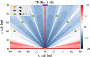
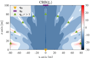
Single target: on a single target, it is expected the highest performance in estimating angle $\alpha$, as depicted in Fig. 1c, mainly when the SP is close the BS and under the lowest at broadside angles. Besides, for estimating of $\xi$ angle, the behavior of the harmonics is the key indicator. We set $m_{f}=3$ and both CRBs calculations are depicted in Fig. 2. This result reveals reliable capacity of the proposed STCM-based method in estimating a single SP position through retrieving intrinsic signal properties and its synthetic harmonic frequencies generated by switching the impinged signal at the metasurface.

(a) Cramer Rao Bounds w.r.t. $\alpha$.

(b) Cramer Rao Bounds w.r.t. $\xi$.

Figure 2: Single target estimation Cramér Rao Bounds. The contour plot, scaled in dB, shows the variance of the estimator given the location of an SP in ${\bf q}_{r}=(x,0,z),x\in[-80:80],z\in[0,100]$ meters.

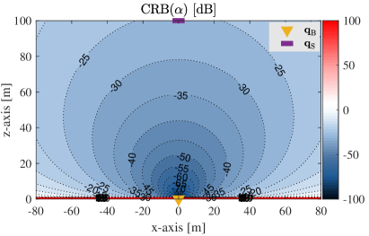
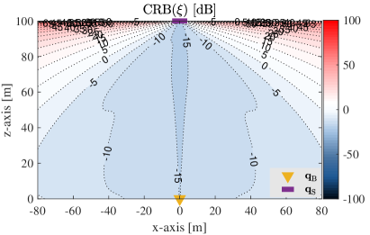
The result of Fig. 2a reveals that the CRB variance for the $\alpha$ angle estimation decreases as $d_{r}$ increases, except for extreme broadside angles. Hence, the localization performance is bounded by the signal-to-noise ratio (SNR) of the signal, involving the propagation characteristics, signals, and transmit power. Moreover, the CRB for the $\xi$ angle estimation is shown to be directly bounded by the directivity of the generated harmonics in the STCM. One can infer that when $\xi\approx 0$ degrees, the variance of the $\xi$ estimates achieves its lowest value. At the same time, the estimator’s variance is higher than 1 when $\xi\gtrapprox 60$ degrees, due to the reflected signal strength in those locations being very attenuated with the employed switching pattern and the number of harmonics [11]. Hence, those parameters associated with switching patterns and the number of harmonics as described in eqs. (3) and (4) can be optimized via Eq. (20).

We stick to the number of harmonics. In Fig. 3, we analyze the CRB variance of $\xi$ using more frequency harmonics of higher orders.

Figure 3: Highest order harmonic $m_{f}$ versus CRB ($\xi$) in [dB], eq. (20), as a function of the STCM-SP angle $\xi$.

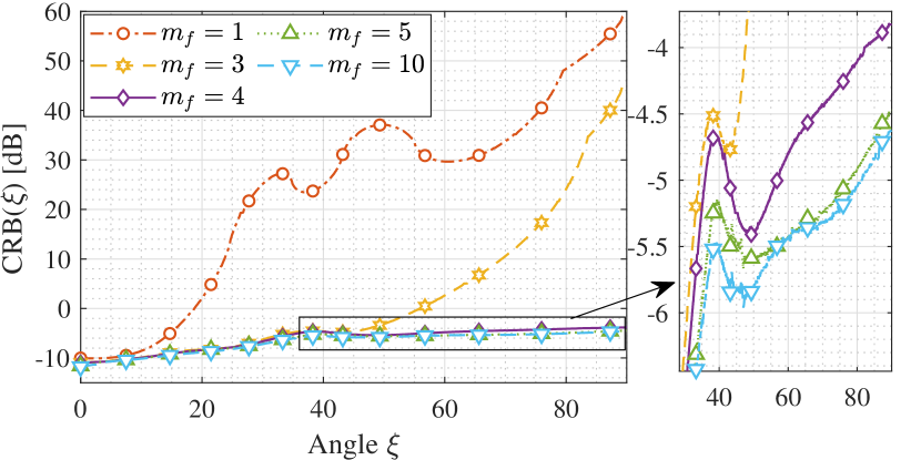
Notice that including more harmonics above $m_{f}=3$ can increase the localization accuracy to the whole analyzed environment (CRB $(\xi)<1,\ \forall\xi$), but does not increase significantly the result for angles lower than $50^{\rm o}$. Moreover, we can see that using more than four harmonics, $m_{f}>4$, does not increase significantly the performance, with just a slight variation of $1$ dB when comparing $m_{f}=4$ to $m_{f}=5$ CRB curves and much lower improvement for $m_{f}=10$ in comparison to $m_{f}=5$. Thus, under this switching pattern, the efficient configuration in complexity and performance is attained when $m_{f}=4$ positive and negative harmonics are deployed. Next, we stress the capability of estimating double and multiple target positions.

Double target: we want to formulate the CRB to evaluate the effect of the mutual interference and limitations of localization estimation in the proposed STCM-assisted M-MIMO system. In this setup, we fix an SP ₂ location in ${\bf q}_{2}=[60,0,40]$ and calculate the CRB for SP ₁ in ${\bf q}_{1}=[q_{x},0,q_{z}]$ position and the CRB for SP ₂ when SP ₁ is in position ${\bf q}_{1}=[q_{x},0,q_{z}]$, respectively. We do this calculation numerically by expanding the FIM s, Eq. (14) and Eq. (18) for the SB and DB configurations, respectively. This result is presented in Fig. 4.

(a) Cramer Rao Bounds w.r.t. $\alpha$ for $|\mathcal{R}|=2$.

(b) Cramer Rao Bounds w.r.t. $\xi$ for $|\mathcal{R}|=2$.

Figure 4: Double target estimation Cramér Rao Bounds. The contour plot shows the variance of the estimator for SP ₁ (left plots) in ${\bf q}_{1}=[x,0,z],x\in[-80,80],z\in[0,100]$ given the location of an SP ₂ in ${\bf q}_{2}=[60,0,40]$ meters. Right plots is the CRB s for SP ₂.

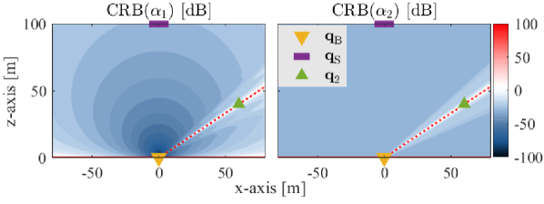
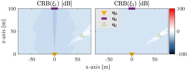
Fig. 4 reveals that the angles estimation CRB when $|\mathcal{R}|>1$ are bounded to the spatial distribution of them. The mutual interference is higher when the SPs share the same BS-SP angle, $\alpha$, and the estimation of $\alpha_{r},\ r=\{1,2\}$, indicates to be either unfeasible or very imprecise, Fig. 4a. The estimation of $\xi_{r}$ is bounded by a region when one SP is placed next to the other, Fig. 4b. However, to precisely localize the SPs, the estimator’s variance must be low for both parameters, showing both circumstances bound the performance.

Multiple targets: let’s stress the system capabilities with a massive number of targets, $|\mathcal{R}|=10$, where nine targets are fixed and deployed equally spaced in a manner to cover the whole range of BS-SP angles, excluding the extremes broadsides, while evaluating the CRBvariance estimate for a target in ${\bf q}_{1}=[x,0,z]$ location. Fig. 5 reinforce physical limitation on precisely estimating the localization when more than one SP is deployed at the same angle, Fig. 5a, or same region, Fig. 5b. In the first case, the contour plot in Fig 5a reveals that the broadside SPs are the ones that make the localization estimation inaccurate or even infeasible (white-to-red and red areas), affecting a much larger region than the rest. In the case of $\xi$ covariance estimation, Fig. 5b corroborates the STCM can overcome the limitations related to the angles and is bounded to a region that is larger for broadside SPs too. Hence, one can conclude that those estimations may not be precise in such locations.

(a) $|\mathcal{R}|=10$ CRB BS-SP angle CRB

(b) $|\mathcal{R}|=10$ STCM-SP angle CRB

Figure 5: Cramer Rao Bounds for (a) $\alpha$ and (b) $\xi$ angles in multiple target $|\mathcal{R}|=10$ case.

To comprehensively evaluate the localization capabilities of the proposed method, in the following subsections we reinterpret the information of the CRB variance of the angles estimates to local coordinates.

IV-A Localization performance

We can see from previous numerical result calculations that an optimal estimator is capable of estimating both angles studied here with a low error covariance, but it does not give us precise information on capabilities. To evaluate the local coordinates localization performance, we translate the information in angles relationship to the PEB, Sect. III-A1. The PEB gives the precise bound of localization in meters considering the information contained in the channel. Hence, let us present in Fig. 6 the PEB for the single, Fig 6a, double, Fig 6b, and multiple targets, 6c, scenarios shown previously.

(a) PEB when a single SP is positioned at ${\bf q}_{r}=(x,z),x\in[-80,80]$ m and $z\in[0,100]$ m.

(b) PEB when an SP is positioned at ${\bf q}_{1}=(x,z),x\in[-80,80]$ m and $z\in[0,100]$ m with a fixed SP at ${\bf q}_{2}=(60,40)$ m.

(c) PEB when anSP is positioned at ${\bf q}_{1}=(x,z),x\in[-80,80]$ m and $z\in[0,100]$ m with a set of fixed SPs equidistributed around the BS (see Fig. 5)

Figure 6: Position Error Bounds for the various number of SPs.

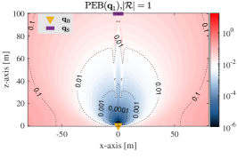
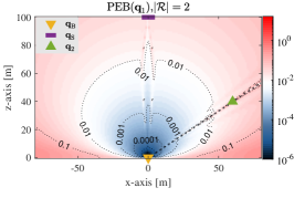
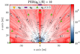
Fig. 6 reinterprets the CRB covariance into localization accuracy in meters where the behavior of the angles estimation variances are reflected in the SP position estimation. The localization performance decreases with $d_{r}$ increasing, Fig. 6a, from micro centimeter level to centimeter level, with a large region below subcentimeter level and, in the worst case for a broadside of both BS and STCM, to tenths-of-centimeter level. With the addition of more SP, we can see that the PEB $\gg 1$ when $\alpha_{1}=\alpha_{2}$, Fig. 6b, being the most significant limitation of the system. Moreover, when $|\mathcal{R}|=10$, the localization is degraded compared to previous cases but still achieves a tenth-of-centimeter PEB level or below for a big area. Hence, the presence of the SP can be viewed as an interference, and this performance may be increased by the successive cancelation of signals or employing different combiners, e.g., zero forcing, once an SP is localized to eliminate its interference from others SP signal. Thus, this is a subject for future work.

IV-B Detection and Classification performance

From the numerical simulations presented in previous subsections, one can affirm that, under certain limitations, the BS is capable of recovering not only the AoA of the SPs but also their position due to characteristics brought by the STCM once they are detected. However, the detection is not immediate and is subject to false alarms. To evaluate the detection capability, let us rely on the framework presented in Section III-B.

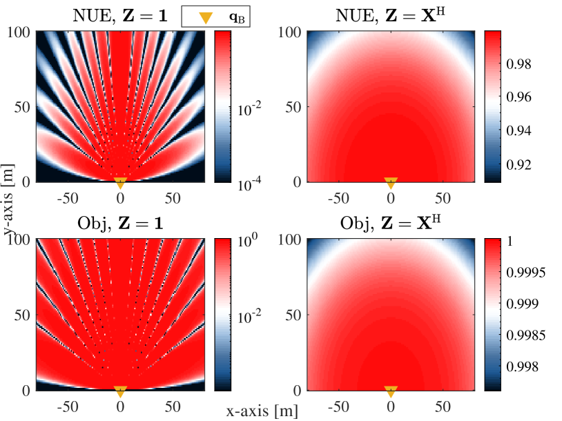
Detection: recall Section III-B, where we assume a known targets’ location ${\bf q}$. We want to evaluate the theoretical detection probability by evaluating Eq. (35) under parameters $\sigma_{i}$ depicted in Table I resembling the NUE and Obj detectability. From Eq. (35), it is straightforwardly inferred that the detection probability is dependent on the noise power, a threshold for detection, the channel state condition, including transmit and combining/receiving beamforming and pilot symbols, and the specific targets’ RCS. Let ${\bf H}({\bf q})$ be defined as

$${\bf H}({\bf q})={\bf Z}{{\bf a}_{\rm B}}(\angle{\bf q}){{\bf a}^{\top}_{\rm B}}(\angle{\bf q}){\bf X}$$ (53)

with ${\bf Z}$ being a special case of combining beamformer having the same dimension as ${\bf X}$ employed in the same manner as de-spreading operation in channel estimation [27]. We use only the direct component c2) since $\bar{\beta}_{r}\gg\bar{\bar{\beta}}_{r}$. We compare two configurations for de-spreading, being i) ${\bf Z}={\bf 1}_{M}$ and ii) ${\bf Z}={\bf X}^{\rm H}$. The position ${\bf q}$ versus probability detection $p_{D}$ is depicted in Fig. 7.

When using the naive combiner i), Fig 7, left subplots, the performance is greatly degraded in comparison with ii), right subplots, which is consistent with physical characteristics of the system. Also, we can notice that the higher the RCS, the higher the detection probability, which can be compared by looking at the color bar ranges depicted in the graphics.

Figure 7: Theoretical detection probability comparison by SP type and combiner under $p_{\rm FA}=10^{-4}$.

Classification: given an SP were detected, we can classify whether it is a false alarm, i.e. $\hat{i}=0$, an NUE, $\hat{i}=1$, or an Obj, $\hat{i}=2$, recalling from the nomenclature defined in Section III-B. We will consider the Special Case: circular covariance and evaluate Eq. (III-C).

We resort to Monte Carlo simulations to present the results in this stage. The setup includes a) for every point in the enclosed space of ${\bf q}_{x}\in[-80,80],{\bf q}_{y}\in[0,100]$ we simulate the existence of one SP of each type separately. Then, we evaluate Eq. (III-C) and solve Eq. (40) to evaluate the classification probability of each type of SP. The numerical results are depicted in Fig. 8.

Figure 8: Classification analysis for an impinging signal reflected on the two types of SP.

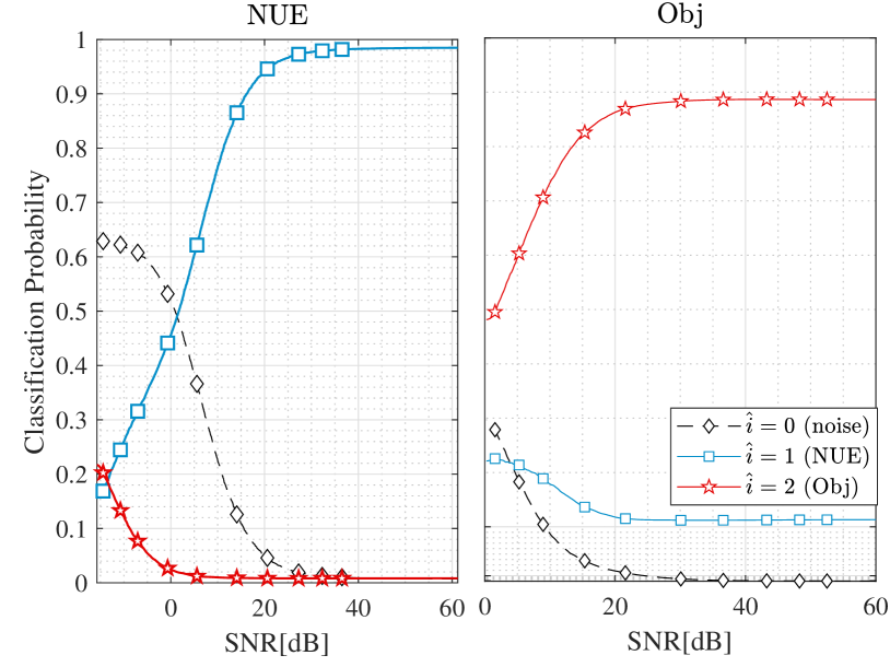
Fig. 8 shows the SP mean SNR $\frac{|{\rm vec}(\bar{\beta}_{r}{\bf H})^{\rm H}{\rm vec}(\bar{\beta}_{r}{\bf H})|}{\sigma_{n}^{2}}$ versus classification probability of a signal reflected on an NUE (left) and in an SP (right). The simulations were performed in the $100\times 160$ squared-meter scenario, with the curves obtained by averaging $10^{4}$ runs of the algorithm. With SNR higher than $20$ dB, the probability of correct classification of NUE signal is above $90$% with a plateau of $98.4926$% after $\approx 35$ dB, while for Obj the plateau is on $88.636$% for SNR s higher than $30$ dB. The probability of misclassification between SPs is low for both cases, approximating zero for high SNR s in the NUE case, but with a floor of $11.2256$% in Obj case. This occurs in higher SNR s, i.e. when the SP is nearer to the BS, being this the region where the Rayleigh distributions of both signals have higher overlap. Below zero SNR the classification as noise is most likely to occur.

IV-C Sensing with RIS

Finally, we evaluate whether it is possible to perform the sensing framework proposed herein by deploying an ordinary metasurface, i.e. that does not perform space-time coding within a single transmission interval. Hence, we reformulate the received signal exchanging the STCM non-linear space-frequency scattering and substitute by the RIS reflecting framework with a fixed elements’ configuration. Hence, Eq. (5) is adapted specifically for angles $\alpha$ and $\xi$, maintaining the static characteristic analyzed before, thus $d_{m}(\tau)=1$.

$$\begin{split}{\bf Y}^{\rm echo}_{\rm RIS}\triangleq\bigg{(}\underbrace{\bar{\beta}_{{\rm S}}{{\bf a}_{\rm B}}(0)({{\bf a}^{\top}_{\rm R}}(0)\boldsymbol{\Omega}{{\bf a}_{\rm R}}(0)){{\bf a}^{\top}_{\rm B}}(0)}_{\text{{\it c1)} BS-RIS-BS}}\\ +\sum\limits_{r\in\mathcal{R}}\underbrace{\bar{\beta}_{r}{{\bf a}_{\rm B}}(\alpha){{\bf a}^{\top}_{\rm B}}(\alpha)}_{\text{{\it c2)} BS-SP-BS}}\\ +\sum\limits_{r\in\mathcal{R}}\underbrace{\bar{\bar{\beta}}_{r}{{\bf a}_{\rm B}}({\alpha})({{\bf a}^{\top}_{\rm R}}({\xi})\boldsymbol{\Omega}{{\bf a}_{\rm R}}(0)){{\bf a}^{\top}_{\rm B}}(0)}_{\text{{\it c3)} BS-RIS-SP-BS}}\\ +\sum\limits_{r\in\mathcal{R}}\underbrace{\bar{\bar{\beta}}_{r}{{\bf a}_{\rm B}}(0)({{\bf a}^{\top}_{\rm R}}(0))\boldsymbol{\Omega}{{\bf a}_{\rm R}}({\xi})){{\bf a}^{\top}_{\rm B}}({\alpha})}_{\text{{\it c4)} BS-SP-RIS-BS}}\bigg{)}{\bf X}+{\bf N},\end{split}$$ (54)

where ${{\bf a}_{\rm R}}(\cdot)\in\mathbb{C}^{N\times 1}$ denotes the RIS array RV and $\boldsymbol{\Omega}={\rm diag}(\boldsymbol{\omega})$, where $\boldsymbol{\omega}=[\omega_{1},\omega_{2},\dots,\omega_{N}]$ is the RIS phase-shift profile. Straightforward, we can retrieve the CRB using the same procedure as described in Sect. III. We suppress the derivations and stick to the result presented in Fig. 9.

Figure 9: CRB in linear RIS assisted sensing.

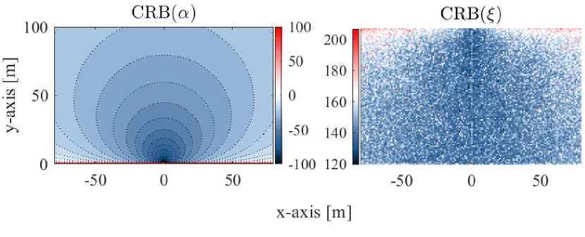
The behavior presented in Fig. 9 shows the incapability of applying the linear metasurface in the proposed approach. The surfaces obtained indicate that it is not possible to retrieve the RIS-SP angle since an estimator variance is as high as 120 dB in the best case. Hence, to produce similar results as obtained with STCM, it would need at least $|\mathcal{M}|$ configurations on the conventional RIS phases profile, thus a huge amount of symbols, to reproduce the frequency-space scattering setups, in which the sensing framework is based. Such a method of operation demands a large amount of resources in the control channel and timing, and may not be feasible to be implemented directly in the ISAC systems due to physical constraints on the channels’ coefficients during a frame. The detection and classification do not rely on harmonic frequencies, and we can infer that RISattains similar or equal performance. Hence, we can conclude that the STCM presents an advancement for resource-efficient sensing design into ISAC applications.

V Conclusions

In this paper, we provide a comprehensive theoretical study on using an STCM as support for sensing, where the potential of detecting, localizing, and classifying them into distinct classes is assessed. The approach envisions future ISAC applications since using STCM has been proved to bring benefits also in communication [13]. The results corroborate that using this kind of non-linear topology for intelligent metasurfaces can provide a subcentimeter to decimeter-level localization accuracy of SPs and a method to effectively retrieve the SPs position in local coordinates can be implemented with tradeoff only in processing by the BS side; hence, integrating sensing and communication without degrading the communication service. Although methods deploying linear intelligent metasurfaces had been proposed for sensing tasks, our proposed approach offers the advantage of using only narrowband pilot signals and the scenario being totally static, not relying on Dopplers’ processing of multiple transmitted symbols with high bandwidth [15]. The field of applications for the proposed method under the generic scenario investigated is vast, including electromagnetic field exposure aware communications, physical layer security, localization-based random access protocols, and precoding design based on environmental information, to name a few. Future works include investigating specific scenarios and developing algorithms to interface the metasurfaces’ topology and the specific use cases.

References

- [1] X. Fang, W. Feng, Y. Chen, N. Ge, and Y. Zhang, “Joint communication and sensing toward 6g: Models and potential of using mimo,” IEEE Internet of Things Journal, vol. 10, no. 5, pp. 4093–4116, 2023.
- [2] X. Cheng, D. Duan, S. Gao, and L. Yang, “Integrated sensing and communications (isac) for vehicular communication networks (vcn),” IEEE Internet of Things Journal, vol. 9, no. 23, pp. 23 441–23 451, 2022.
- [3] L. Ma, J. Lu, C. Gu, and J. Mao, “A wideband dual-circularly polarized, simultaneous transmit and receive (star) antenna array for integrated sensing and communication in iot,” IEEE Internet of Things Journal, vol. 10, no. 7, pp. 6367–6376, 2023.
- [4] Y. Du, Y. Liu, K. Han, J. Jiang, W. Wang, and L. Chen, “Multi-user and multi-target dual-function radar-communication waveform design: Multi-fold performance tradeoffs,” IEEE Transactions on Green Communications and Networking, vol. 7, no. 1, pp. 483–496, 2023.
- [5] M. Zhang, Y. He, Y. Cai, G. Yu, and N. Al-Dhahir, “Design and performance analysis of wireless legitimate surveillance systems with radar function,” IEEE Transactions on Communications, vol. 71, no. 4, pp. 2517–2531, 2023.
- [6] B. Sun, B. Tan, M. Ashraf, M. Valkama, and E. S. Lohan, “Embedding the localization and imaging functions in mobile systems: An airport surveillance use case,” IEEE Open Journal of the Communications Society, vol. 3, pp. 1656–1671, 2022.
- [7] J. Mu, W. Ouyang, Z. Jing, B. Li, and F. Zhang, “Energy-efficient interference cancellation in integrated sensing and communication scenarios,” IEEE Transactions on Green Communications and Networking, vol. 7, no. 1, pp. 370–378, 2023.
- [8] F. Liu, Y. Cui, C. Masouros, J. Xu, T. X. Han, Y. C. Eldar, and S. Buzzi, “Integrated sensing and communications: Toward dual-functional wireless networks for 6g and beyond,” IEEE Journal on Selected Areas in Communications, vol. 40, no. 6, pp. 1728–1767, 2022.
- [9] X. Wang, Z. Fei, and Q. Wu, “Integrated sensing and communication for ris-assisted backscatter systems,” IEEE Internet of Things Journal, vol. 10, no. 15, pp. 13 716–13 726, 2023.
- [10] G. B. Wu, J. Y. Dai, K. M. Shum et al., “A universal metasurface antenna to manipulate all fundamental characteristics of electromagnetic waves,” Nature Communications, vol. 14, p. 5155, 2023.
- [11] L. Zhang, X. Q. Chen, Q. Z. Shuo Liu, J. Zhao, J. Y. Dai, G. D. Bai, X. Wan, Q. Cheng, and T. J. Cui, “Space-time-coding digital metasurfaces,” Nat Commun, vol. 9, no. 4334, 2018.
- [12] J. Y. Dai, W. Tang, L. X. Yang, X. Li, M. Z. Chen, J. C. Ke, Q. Cheng, S. Jin, and T. J. Cui, “Realization of multi-modulation schemes for wireless communication by time-domain digital coding metasurface,” IEEE Transactions on Antennas and Propagation, vol. 68, no. 3, pp. 1618–1627, 2020.
- [13] J. Yuan, E. De Carvalho, R. J. Williams, E. Björnson, and P. Popovski, “Frequency-mixing intelligent reflecting surfaces for nonlinear wireless propagation,” IEEE Wireless Communications Letters, vol. 10, no. 8, pp. 1672–1676, 2021.
- [14] F. Saggese, V. Croisfelt, R. Kotaba, K. Stylianopoulos, G. C. Alexandropoulos, and P. Popovski, “On the impact of control signaling in ris-empowered wireless communications,” 2023.
- [15] H. Kim, A. Fascista, H. Chen, Y. Ge, G. C. Alexandropoulos, G. Seco-Granados, and H. Wymeersch, “Ris-aided radar sensing and object detection with single and double bounce multipath,” 2022.
- [16] K. Keykhosravi, M. F. Keskin, G. Seco-Granados, P. Popovski, and H. Wymeersch, “RIS-Enabled SISO Localization Under User Mobility and Spatial-Wideband Effects,” IEEE Journal of Selected Topics in Signal Processing, vol. 16, no. 5, pp. 1125–1140, 2022.
- [17] H. Wymeersch and G. Seco-Granados, “Radio localization and sensing—part i: Fundamentals,” IEEE Communications Letters, vol. 26, no. 12, pp. 2816–2820, 2022.
- [18] R. E. Jarvis, R. G. Mattingly, and J. W. McDaniel, “Uhf-band radar cross section measurements with single-antenna reflection coefficient results,” IEEE Transactions on Instrumentation and Measurement, vol. 70, pp. 1–4, 2021.
- [19] T. V. Tien, L. Ouvry, and A. Sibille, “Time domain complex radar cross section of human body for breath-activity monitoring,” in 2017 11th European Conference on Antennas and Propagation (EUCAP), 2017, pp. 421–425.
- [20] D. Fontanelli, F. Shamsfakhr, and L. Palopoli, “Cramer–rao lower bound attainment in range-only positioning using geometry: The g-wls,” IEEE Transactions on Instrumentation and Measurement, vol. 70, pp. 1–14, 2021.
- [21] Z. Abu-Shaban, X. Zhou, T. Abhayapala, G. Seco-Granados, and H. Wymeersch, “Error bounds for uplink and downlink 3D localization in 5G millimeter wave systems,” IEEE Transactions on Wireless Communications, vol. 17, no. 8, pp. 4939–4954, 2018.
- [22] H. Wymeersch and G. Seco-Granados, “Adaptive detection probability for mmWave 5G SLAM,” in 2020 2nd 6G Wireless Summit (6G SUMMIT), 2020, pp. 1–5.
- [23] P. Sofotasios, M. Valkama, T. Tsifitsis, Y. Brychkov, S. Freear, and G. Karagiannidis, “Analytic solutions to a marcum q-function-based integral and application in energy detection of unknown signals over multipath fading channels,” in 2014 9th International Conference on Cognitive Radio Oriented Wireless Networks and Communications (CROWNCOM). IEEE, 7 2014.
- [24] S. Kay, Fundamentals of Statistical Signal Processing: Detection theory, ser. Fundamentals of Statistical Si. Prentice-Hall PTR, 1998.
- [25] A. Khawar, A. Abdelhadi, and C. Clancy, “Target detection performance of spectrum sharing MIMO radars,” IEEE Sensors Journal, vol. 15, no. 9, pp. 4928–4940, 2015.
- [26] I. Bekkerman and J. Tabrikian, “Target detection and localization using mimo radars and sonars,” IEEE Transactions on Signal Processing, vol. 54, no. 10, pp. 3873–3883, 2006.
- [27] T. L. Marzetta, E. G. Larsson, H. Yang, and H. Q. Ngo, Fundamentals of Massive MIMO. Cambridge University Press, 2016.