IFT-UAM/CSIC-23-60

Machine-Learning Performance on
Higgs-Pair Production associated with Dark Matter at the LHC

Ernesto Arganda¹, Manuel Epele², Nicolas I. Mileo², and Roberto A. Morales²

¹Departamento de Física Teórica and Instituto de Física Teórica UAM-CSIC,
Universidad Autónoma de Madrid, Cantoblanco, 28049 Madrid, Spain

²IFLP, CONICET - Dpto. de Física, Universidad Nacional de La Plata,
C.C. 67, 1900 La Plata, Argentina

Di-Higgs production at the LHC associated with missing transverse energy is explored in the context of simplified models that generically parameterize a large class of models with heavy scalars and dark matter candidates. Our aim is to figure out the improvement capability of machine-learning tools over traditional cut-based analyses. In particular, boosted decision trees and neural networks are implemented in order to determine the parameter space that can be tested at the LHC demanding four $b$-jets and large missing energy in the final state. We present a performance comparison between both machine-learning algorithms, based on the maximum significance reached, by feeding them with different sets of kinematic features corresponding to the LHC at a center-of-mass energy of 14 TeV. Both algorithms present very similar performances and substantially improve traditional analyses, being sensitive to most of the parameter space considered for a total integrated luminosity of 1 ab^-1, with significances at the evidence level, and even at the discovery level, depending on the masses of the new heavy scalars. A more conservative approach with systematic uncertainties on the background of 30% has also been contemplated, again providing very promising significances.

1 Introduction

In the last few years machine learning (ML) has become an standard and basic tool for experimental and phenomenological high-energy physics studies (for reviews see, for instance, [1, 2, 3, 4, 5, 6, 7, 8, 9, 10, 11]). Indeed, ML may be crucial to take full advantage of the data collected at the LHC in order to probe the standard model (SM) and new physics. In this sense, a key issue is whether ML techniques could replace traditional counting methods based on rectangular cuts. The ATLAS and CMS Collaborations have shown in many experimental analyses the potential of ML tools, as boosted decision trees (BDT) and neural networks (NN), to improve the LHC sensitivity, understood as the signal-to-background ratio, to beyond the SM (BSM) physics [12, 13, 14, 15, 16, 17, 18, 19, 20, 21, 22, 23, 24, 25, 26, 27, 28, 29, 30, 31, 32, 33, 34, 35, 36, 37, 38, 39, 40, 41, 42, 43, 44, 45, 46, 47, 48, 49, 50, 51, 52, 53, 54, 55]. The main goal of this work is to find out the improvement capability of modern ML tools over cut-based analyses applied to a case study of physical interest: the production at the LHC of Higgs boson pairs associated with dark matter (DM) particles.

After the Higgs boson discovery [56, 57], with a mass value of $m_{h}$ = 125.09 $\pm$ 0.24 GeV [58] and which seems to be the scalar Higgs boson predicted by the SM [59], the search for extended Higgs sectors represents an intensive experimental program carried out at the LHC by ATLAS and CMS (for recent analyses see, for instance, [60, 61, 62, 63, 64, 65, 66, 67, 68, 69, 70, 71, 72, 73, 74, 75, 76, 77, 78, 79, 44, 80, 81, 82, 50, 83, 84]). Interestingly, these additional Higgs bosons may serve as portals to dark sectors [85, 86, 87, 88, 89, 90, 91, 92, 93, 94, 95, 96, 97, 98, 99, 100, 101, 102, 103], which could manifest in multi-Higgs final states with a large amount of missing transverse energy ($E_{T}^{\text{miss}}$), coming from the potential emission of DM that escapes from the LHC detectors. In fact, ATLAS and CMS are also conducting many searches for di-Higgs production plus $E_{T}^{\text{miss}}$ [104, 105, 106, 107, 108, 109, 110, 72, 111, 112, 113].

In the context of these di-Higgs + $E_{T}^{\text{miss}}$ searches at the LHC, numerous phenomenological collider analyses have emerged [114, 115, 116, 117, 118, 119, 120, 121, 122, 123, 124, 125, 126]. Based on the search strategies developed in [121] and motivated by the use of multivariate analysis (MVA) tools in [125] and [126], in this work we aim to study the performance of modern ML algorithms on this type of phenomenological analyses. Concretely, in order to try to increase the LHC sensitivity to di-Higgs + $E_{T}^{\text{miss}}$ signatures in general frameworks of extended Higgs sectors, we will employ the XGBoost toolkit [127, 128] and deep neural networks (DNN) [129, 130, 131, 132].

In particular, we work within a general framework defined by simplified models based on effective couplings and interaction terms, inspired by [125], and consider the resonant production of a pair of heavy scalars at the LHC, with one of the heavy scalar decaying invisibly to a pair of DM particles, and the other one decays to two SM-like Higgs bosons, which subsequently decay to bottom-quark pairs as in [121]. Therefore, the LHC signature under study consists of 4 $b$-jets plus a large amount of $E_{T}^{\text{miss}}$, whose dominant irreducible backgrounds are $Zb\bar{b}b\bar{b}$ and $t\bar{t}b\bar{b}$. We will define several benchmarks, covering the region of the parameter space of interest, with different kinematic characteristics, and train the ML algorithms with balanced signal and background event samples for each. We will maximize the signal significance for each benchmark, including a rough estimation of the systematic uncertainties, scanning over the different values of the ML classifier scores. We will also compare the performances of XGBoost and DNN with respect to traditional cut-based search strategies.

The paper is structured as follows: in Section 2 we introduce the simplified BSM model that produces the LHC signature under study, define the signal benchmarks and present the collider variables with which we feed the ML algorithms to discriminate between signal and background; Section 3 is devoted to summarize the main features of XGBoost and DNN algorithms used for differentiating signal to background; Section 4 is dedicated to the analysis of the XGBoost and DNN performances compared to the rectangular cut-based collider analyses; finally, we leave Section 5 to discuss our main conclusions.

2 Phenomenological Framework

We start our analysis of di-Higgs + $E_{T}^{\text{miss}}$ production at the LHC, with a center-of-mass energy of 14 TeV and a luminosity of $\cal{L}$ = 1 ab^-1, in the context of a general class of simplified models, inspired by the effective couplings and interactions terms presented in [125]. This class of models relies on an extended scalar sector with three real scalar particles. The heaviest of these new scalars, $\upphi$, is produced via gluon fusion at the LHC (through an effective dimension-five interaction) and predominantly decays to a pair of intermediate scalars $\upvarphi$. This scalar interacts with the visible sector only through its coupling with the SM Higgs boson $h$. The lightest scalar $\chi$ is the DM candidate within the framework of this effective field theory. We consider only the resonant topology $pp\to\upphi\to\upvarphi\upvarphi\to(hh)(\chi\chi)$ since it is the most pessimistic scenario presented in [125] and the necessity of ML algorithms is well motivated. This topology is shown in Figure 1 and is also very similar to one studied in our previous work [121]. In particular we consider a variety of benchmarks of this class of simplified models scanning the mass $m_{\upphi}$ of the heavy scalar in the range [750, 1500] GeV and the mass $m_{\upvarphi}$ of the intermediate state in the range [275, $m_{\upphi}/2$] GeV .

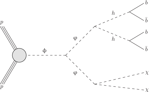
Figure 1: Decay chain topology of LHC production of a heavy scalar $\upphi$, that decays into a pair of intermediate scalars $\upvarphi$. One of the scalar $\upvarphi$ decays into a pair of SM-like Higgs bosons $h$, which subsequently decay into $b$-quark pairs, whilst the other scalar $\upvarphi$ decays directly into a pair of DM candidates, the lightest scalar $\chi$.

The interaction Lagrangian for this simplified model is given by

$$\mathcal{L}=\frac{C_{\upphi gg}}{\Lambda}\upphi G_{\mu\nu}G^{\mu\nu}+\frac{m_{\upphi\upvarphi\upvarphi}}{2}\upphi\upvarphi\upvarphi+\frac{m_{\upvarphi hh}}{2}\upvarphi hh+\frac{m_{\upvarphi\chi\chi}}{2}\upvarphi\chi\chi\,,$$ (1)

and the resulting cross section for the topology in Figure 1 is factorized as

$$\sigma(pp\to b\bar{b}b\bar{b}\chi\chi)=\sigma(pp\to\upphi)\cdot\text{BR}(\upphi\to\upvarphi\upvarphi)\cdot 2\cdot\text{BR}(\upvarphi\to hh)\cdot\text{BR}(\upvarphi\to\chi\chi)\cdot\left[\text{BR}(h\to b\bar{b})\right]^{2}\,.$$ (2)

Following [125], the effective coupling $C_{\upphi gg}$ collects the effect of heavy quarks at scale $\Lambda=1$ TeV (well above the EW scale $v=246$ GeV) in an UV complete theory and the production cross section $\sigma(pp\to\upphi)$ can be obtained from the LHC Higgs cross-section working group for BSM scalars $S$ [135]:

$$\sigma(pp\to\upphi)=\left(\frac{v}{1\,\text{TeV}}\right)^{2}\sigma(pp\to S)\,.$$ (3)

We are interested in the kinematic region corresponding to the mass of the heavy scalar larger than twice the mass of the intermediate scalar. Then the two decay channels for the heavy scalar are

$$\Gamma(\upphi\to\upvarphi\upvarphi)=\frac{m_{\upphi\upvarphi\upvarphi}^{2}}{32\pi m_{\upphi}}\sqrt{1-\frac{4m_{\upvarphi}^{2}}{m_{\upphi}^{2}}}\quad\text{and}\quad\Gamma(\upphi\to gg)=\frac{C_{\upphi gg}^{2}}{1\,\text{TeV}^{2}}\frac{2m_{\upphi}^{3}}{\pi}\,.$$ (4)

Setting the coupling $m_{\upphi\upvarphi\upvarphi}$ equal to the EW scale $v=246$ GeV and far to the $\upvarphi\upvarphi$ threshold, we have BR$(\upphi\to\upvarphi\upvarphi)\sim 1$.

In addition, the couplings $m_{\upvarphi hh}$ and $m_{\upvarphi\chi\chi}$ are such that the branching ratios of $\upvarphi$ decaying to $hh$ and $\chi\chi$ maximize their product. Concretely, we fix BR$(\upvarphi\to hh)$ = BR$(\upvarphi\to\chi\chi)=0.5$. We consider also BR$(h\to b\bar{b})$ = 0.58 [136].

Signal and background events are generated with MadGraph_aMC@NLO 2.8.1 [137], the parton showering and hadronization is carried out by using PYTHIA 8.2 [138], and the detector response is simulated through Delphes 3.3.3 [139, 140, 141], with the jets being reconstructed with FastJet 3.4.0 [142, 143]. We use the default setup for the ATLAS detector provided by Delphes 3.3.3, in which the $b$-tagging efficiency, and the light and charm jet mistag rates are given by

$$\epsilon_{b}=\frac{24\tanh(0.003\,p_{T})}{1+0.086\,p_{T}}\,,\quad\epsilon_{j}=0.002+7.3\times 10^{-6}\,p_{T}\,,\quad\epsilon_{c}=\frac{0.2\,\tanh(0.02\,p_{T})}{1+0.0034\,p_{T}}\,,$$ (5)

respectively. With this working point a maximum $b$-tagging efficiency of $\sim 73\%$ is reached for a jet transverse momentum of $p_{T}\sim 120$ GeV. We work in the 4-flavor scheme and we do not apply jet matching since we do not have light jets in the hard process of our signal. The simulation input files and the internal analysis codes are available upon request to the authors.

We focus on a signal region defined by imposing the following cuts at detector level:

$$N_{b}=4\,,\quad N_{lep}=0\,,\quad p_{T}^{j,b}>20\,\text{GeV}\,,\quad E_{T}^{\text{miss}}>200\,\text{GeV}\,,$$ (6)

where $N_{b}$ and $N_{lep}$ are the number of $b$-jets and leptons (electrons and muons), respectively, $p_{T}^{j,b}$ is the transverse momentum of light and $b$-tagged jets, and $E_{T}^{\text{miss}}$ is the transverse missing energy. In particular, the lepton-veto disfavors the presence of missing energy coming from neutrinos in the top-quark decays.

For each benchmark, the acceptance $\varepsilon_{\text{SR}}$ is the fraction of the simulated signal events which satisfy Eq. (6). Combining this quantity with Eq. (2), the effective cross section is defined as $\sigma_{\text{eff}}=\sigma(pp\to b\bar{b}b\bar{b}\chi\chi)\cdot\varepsilon_{\text{SR}}$ and, after multiplying by the luminosity, it represents the number of expected signal events in the signal region of Eq. (6). The effective cross sections for the 14 simulated benchmarks are shown in Figure 2 by red points in the plane $[m_{\upphi},m_{\upvarphi}]$. For fixed heavy scalar mass $m_{\upphi}$, the cross section is roughly $m_{\upvarphi}$ independent. However, the acceptance $\varepsilon_{\text{SR}}$ becomes smaller for low $m_{\upvarphi}$ and also close to the threshold, $m_{\upvarphi}\sim m_{\upphi}/2$, leading to the profile of the effective cross section observed in this figure. In particular, near the threshold, both scalars $\upvarphi$ are produced almost at rest, which strongly reduces the acceptance $\epsilon_{\mathrm{SR}}$ due to the impact of the missing transverse energy cut. On the other hand, when $m_{\upvarphi}$ is close to the production threshold of two Higgs bosons from the decay of $\upvarphi$, these emerge almost at rest in the $\upvarphi$-frame and then they are emitted roughly along the direction of the momentum of $\upvarphi$ in the collision frame, which make their decay products more difficult to resolve. Thus, the acceptance $\epsilon_{\mathrm{SR}}$ decreases significantly when demanding four $b$-jets. As an example, the acceptance of requiring $N_{b}=4$ drops from 0.9 to 0.02 when going from benchmark 1250_475_25 to 1250_275_25 .

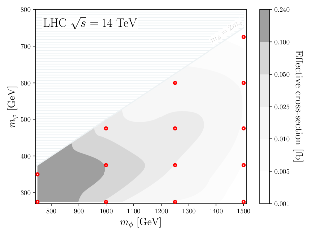
Figure 2: Effective cross section in the plane $[m_{\upphi},m_{\upvarphi}]$ defined as $\sigma_{\text{eff}}=\sigma(pp\to b\bar{b}b\bar{b}\chi\chi)\cdot\varepsilon_{\text{SR}}$. The region with $m_{\upphi}<2m_{\upvarphi}$ is kinematically closed. Red points correspond to the benchmarks with events simulated for the training.

Given the topology of the final state and the cuts introduced in Eq. (6), the dominant irreducible SM backgrounds are $Z+b\bar{b}b\bar{b}$, with the invisible decay of the $Z$ boson ($Z\to\nu\bar{\nu}$), and $t\bar{t}+b\bar{b}$, with the semi-leptonic decay modes $t(\to bjj)\bar{t}(\to\bar{b}\ell^{-}\bar{\nu})$ and $t(\to b\ell^{+}\nu)\bar{t}(\to\bar{b}jj)$ of the top-antitop pair. From now on, we denote them as $Z|_{\rm inv}b\bar{b}b\bar{b}$, and $t\bar{t}|_{\rm semilep}b\bar{b}$ and $t\bar{t}|_{\rm semitau}b\bar{b}$ for the semi-leptonic modes of the $t\bar{t}b\bar{b}$ background with $\ell=e,\mu$ and $\ell=\tau$, respectively. On the other hand, the major reducible backgrounds correspond to $t\bar{t}$ and $V$+jets (concretely $Z+b\bar{b}+jj$, $Z+jjjj$, $W^{\pm}+b\bar{b}+jj$ and $W^{\pm}+jjjj$). Notice that the main source of missing transverse energy for these backgrounds are the neutrinos coming from the gauge bosons and $t\bar{t}$ decay channels. In this regard, we safely neglect the QCD multijet production since it does not have a genuine source of missing transverse energy.

Therefore, with the intention of reducing the large background cross sections and making event generation more efficient, we impose the following generator-level cuts on the $p_{T}$ of the light jets and $b$-jets and also to the missing transverse energy  for the background simulation:

$$p_{T}^{b}>20\,\text{GeV}\,,\quad p_{T}^{j}>20\,\text{GeV}\,,\quad E_{T}^{\text{miss}}>200\,\text{GeV}\,.$$ (7)

Taking this into account we only keep the three dominant irreducible backgrounds and two of the reducible $V$+jets category. With the cuts in Eq. (7), the relevant cross sections are

$$\sigma(t\bar{t}|_{\rm semilep}b\bar{b})=33.4\,\text{fb}\,,\quad\sigma(t\bar{t}|_{\rm semitau}b\bar{b})=16.7\,\text{fb}\,,\quad\sigma(Z|_{\rm inv}b\bar{b}b\bar{b})=3.7\,\text{fb}\,,$$

$$\sigma(Z|_{\rm inv}b\bar{b}jj)=937\,\text{fb}\,,\quad\sigma(W^{\pm}|_{\rm semilep}b\bar{b}jj)=373\,\text{fb}\,.$$ (8)

With all the above considerations, we focus our ML analysis in a particular signal region demanding at detector level the Eq. (6). The detector-level events are converted into data arrays, which are to be used as inputs for the ML algorithms, as follows:

• We reconstruct the Higgs bosons from the two $b\bar{b}$ pairs that minimize

  $$\chi_{hh}=\sqrt{\left(\frac{m_{2b}^{\rm lead}-m_{h}}{0.1m_{2b}^{\rm lead}}\right)^{2}+\left(\frac{m_{2b}^{\rm subl}-m_{h}}{0.1m_{2b}^{\rm subl}}\right)^{2}}\,,$$ (9)

  defined in analogy with Ref. [144] ($m_{2b}^{\rm lead(subl)}$ represent the leading (subleading) Higgs boson candidate mass from the $b\bar{b}$ pairs). Then we order these Higgs bosons according to their transverse momentum ($Hst$ and $Hnd$).

• We work with 15 low-level features (shown in Table 1) that characterize the final state at detector level.

• We work with 18 high-level features as shown in Table 2. They are built from the previous low-level features and from the reconstructed (reco) Higgs bosons.

Low-level feature	Description
$N_{j}$	Number of light-jets
$p_{T}^{i}$	Transverse momentum of the four leading $b$-jets ($i=bst,\,bnd,\,brd,\,bth$)
$\eta^{i}$	Pseudorapidity of the four leading $b$-jets ($i=bst,\,bnd,\,brd,\,bth$)
$\phi^{i}$	Azimuthal angle of the four leading $b$-jets ($i=bst,\,bnd,\,brd,\,bth$)
$E_{T}^{\text{miss}}$	Missing transverse momentum
$\phi^{\text{miss}}$	Azimuthal angle of the missing transverse momentum

Table 1: List of low-level features implemented as input variables of our ML classifiers.

High-level feature	Description
$\chi_{hh}$	Defined in Eq. (9)
$p_{T}^{i}$	Transverse momentum of the two reco Higgs bosons ($i=Hst,\,Hnd$)
$\eta^{i}$	Pseudorapidity of the two reco Higgs bosons ($i=Hst,\,Hnd$)
$\phi^{i}$	Azimuthal angle of the two reco Higgs bosons ($i=Hst,\,Hnd$)
$m_{hh}$	Invariant mass of the reco Higgs boson pair
$\Delta\eta_{hh}$	Difference $\eta^{Hst}-\eta^{Hnd}$ of the two reco Higgs bosons
$\Delta\phi_{hh}$	Difference $\phi^{Hst}-\phi^{Hnd}$ of the two reco Higgs bosons
$\Delta R_{hh}$	Distance $\sqrt{\Delta\eta_{hh}^{2}+\Delta\phi_{hh}^{2}}$ of the two reco Higgs bosons
$\Delta\phi_{MET}^{i}$	Differences $\phi^{\text{miss}}-\phi^{i}$ for $i=bst,\,bnd,\,brd,\,bth,\,Hst,\,Hnd$
$E_{T}^{\text{miss}}$ significance	Computed as $E_{T}^{\text{miss}}/\sqrt{p_{T}^{bst}+p_{T}^{bnd}+p_{T}^{brd}+p_{T}^{bth}}$

Table 2: List of high-level features implemented as input variables of our ML classifiers. Here, reco means reconstructed.

We close this Section with a brief discussion of the cut-based analysis, i.e. traditional counting methods based on rectangular cuts, applied to the effective models. Based on the search strategies developed in [121], we present two cases as examples: 750_350_25 and 1000_275_25. We consider the significance with $\Delta=15\%$ of systematic uncertainty as [145]

$$\mathcal{S}_{\text{sys}}=\sqrt{2\left((B+S)\log\left(\frac{\left(\Delta^{2}B^{2}+B\right)(B+S)}{\Delta^{2}B^{2}(B+S)+B^{2}}\right)-\frac{1}{\Delta^{2}}\log\left(\frac{\Delta^{2}B^{2}S}{B\left(\Delta^{2}B^{2}+B\right)}+1\right)\right)}\,,$$ (10)

where $S$ and $B$ are the number of signal and total background events at the end of the search strategy with a luminosity of $\cal{L}$ = 1 ab^-1. Using a cut and count analysis, these two benchmarks are the only ones that exceed evidence (3$\sigma$) significance level.

For 750_350_25, in addition to the cuts in Eq. (6), we demand

$$N_{j}\leq 4\,,\quad p_{T}^{bst}<160\,\text{GeV}\,,\quad p_{T}^{bnd}<110\,\text{GeV}\,,\quad p_{T}^{brd}<80\,\text{GeV}\,,$$

$$\chi_{hh}<3.5\,,\quad m_{hh}<380\,\text{GeV}\,,\quad|\Delta\phi_{MET}^{bst}|<1.8\,,$$ (11)

resulting in $S=22.5$ and $B=16.9$ with a significance of 3.77$\sigma$. In addition, the corresponding distributions are collected in Figure 8 of Appendix A.

On the other hand, for 1000_275_25, in addition to the cuts in Eq. (6), we demand

$$N_{j}\leq 2\,,\quad\chi_{hh}<3\,,\quad m_{hh}<300\,\text{GeV}\,,\quad\Delta R_{hh}<1\,,$$ (12)

resulting in $S=11.6$ and $B=6$ with a significance of 3.48$\sigma$.

3 Machine-Learning Algorithms for Collider Analyses

In order to tackle the binary classification problem we consider two ML algorithms, BDTs and DNNs, and study their performance in discriminating the new physics signal from the SM backgrounds. Before going into the results we provide a brief overview of the gradient-boosted trees, which is the ensemble method XGBoost is based on, and also of neural networks. In addition, we describe the training procedure used in each case.

3.1 XGBoost Overview and Architecture

The discussion in this section follows closely the XGBoost documentation [127] and Ref. [146]. The XGBoost machine learning algorithm is used for supervised learning problems. There are two basic elements in supervised learning: the model and the cost or objective function. The model is the mapping between the training data $\mathbf{x}_{i}$, which involves multiple features, and the target variable $y_{i}$ to be predicted. The parameters of this mapping are learned from data by training the model, which amounts to minimizing an objective function. Once the parameters are obtained, the model provides predictions $\hat{y}_{i}$ of the target variable for each data point $\mathbf{x}_{i}$. Of course, the model can then be used to classify unlabeled inputs. The objective function contains two terms: the training loss function $l(y_{i},\hat{y}_{i})$, that measures how predictive the model is for each data point of the training set, and a regularization term $\Omega$ that does not depend on the data and controls the complexity of the model, which is useful to avoid overfitting.

In XGBoost the model is an ensemble of classification and regression trees (CART). The prediction of the ensemble for a data point $(y_{i},\mathbf{x}_{i})$ is given by

$$\hat{y}_{i}=\sum_{k=1}^{K}f_{k}(\mathbf{x}_{i})\,,$$ (13)

where $K$ is the number of trees in the ensemble and $f_{k}$ is a function in the functional space $\mathcal{F}$ of all possible CARTs. On the other hand, the objective function can be written as

$$\mathrm{obj}=\sum_{i=1}^{N}l(y_{i},\hat{y}_{i})+\sum_{k=1}^{M}\Omega(f_{k})\,,$$ (14)

where $i$ runs over the data points. In order to build the ensemble in Eq. (13) an iterative strategy is applied by adding one new tree at a time. A family of predictors $\hat{y}^{(n)}_{i}$ can be defined as

$$\hat{y}^{(n)}_{i}=\sum_{k=1}^{n}f_{k}(\mathbf{x}_{i})=\hat{y}^{(n-1)}_{i}+f_{n}(\mathbf{x}_{i})\,,$$ (15)

and then the corresponding objective function is given by

$$\mathrm{obj}_{n}=\sum_{i=1}^{N}l(y_{i},\hat{y}^{(n-1)}_{i}+f_{n}(\mathbf{x}_{i}))+\sum_{k=1}^{n}\Omega(f_{k})\,.$$ (16)

By assuming that the adding of a new tree is a small perturbation to the predictor, the loss function can be Taylor expanded to second order to obtain:

$$\mathrm{obj}_{n}\approx\mathrm{obj}_{n-1}+\Delta\mathrm{obj}_{n}\,,$$ (17)

with

$$\Delta\mathrm{obj}_{n}=\sum^{N}_{i=1}g_{i}f_{n}(\mathbf{x}_{i})+\frac{1}{2}h_{i}f_{n}(\mathbf{x}_{i})^{2}+\Omega(f_{n})\,,$$ (18)

where $g_{i}$ y $h_{i}$ are defined as

$$g_{i}=\partial_{\hat{y}^{(n-1)}_{i}}l(y_{i},\hat{y}^{(n-1)}_{i})\,,$$ (19)

$$h_{i}=\partial^{2}_{\hat{y}^{(n-1)}_{i}}l(y_{i},\hat{y}^{(n-1)}_{i})\,.$$ (20)

The $n$-th decision tree in the ensemble $f_{n}$ is then chosen to minimize $\Delta\mathrm{obj}_{n}$, which takes $g_{i}$ and $h_{i}$ as inputs.

In order to specify the regularization term and to obtain an analytical expression for the parameters minimizing $\Delta\mathrm{obj}_{n}$, the following convenient parameterization of the decision trees is introduced:

$$f_{j}(\mathbf{x}_{i})=w_{q(\mathbf{x}_{i})}\,,$$ (21)

where $f_{j}(\mathbf{x}_{i})$ is the prediction of the $j$-th tree for the data point $\mathbf{x_{i}}$, $q(\mathbf{x})$ is a function that assigns each data point to one of the $T$ leaves of the tree, $q:\mathbf{x}\in\mathbb{R}^{d}\to\{1,2,...,T\}$, and $w\in\mathbb{R}^{T}$ is a vector of weights on leaves. With this parameterization, the regularization term can be written as

$$\Omega(f)=\gamma T+\frac{1}{2}\lambda\sum^{T}_{j=1}w^{2}_{j}\,,$$ (22)

with the parameters $\gamma$ and $\lambda$ controlling the penalty for having large partitions with many leaves and large weights on the leaves, respectively .

By using Eq. (21) the Eq. (18) becomes

$$\Delta\mathrm{obj}_{n}=\sum^{T}_{j=1}[G_{j}w_{j}+\frac{1}{2}(H_{j}+\lambda w^{2}_{j})]+\gamma T\,,$$ (23)

where $G_{j}=\sum_{i\in I_{j}}g_{i}$ and $H_{j}=\sum_{i\in I_{j}}h_{i}$, with $I_{j}=\{i|q(\mathbf{x}_{i})=j\}$ the set of indices of data points assigned to the $j$-th leaf. The optimal weights are found to be

$$w^{\mathrm{opt}}_{j}=-\frac{G_{j}}{H_{j}+\lambda}\,,$$ (24)

and the best reduction in the objective is then given by

$$\Delta\mathrm{obj}^{\mathrm{opt}}_{n}=-\frac{1}{2}\sum^{T}_{j=1}\frac{G^{2}_{j}}{H_{j}+\lambda}+\gamma T\,.$$ (25)

Ideally, one would list all the possible trees and select the one that minimizes $\Delta\mathrm{obj}^{\mathrm{opt}}_{n}$. However, this is not possible from a practical point of view. Instead, an approximate algorithm that optimizes one level of the tree at a time is applied. Specifically, optimal splits of leaves are sought by computing the corresponding gain in $\Delta\mathrm{obj}^{\mathrm{opt}}_{n}$. This procedure allows to obtain the structure of a tree that is a good local minimum of $\Delta\mathrm{obj}^{\mathrm{opt}}_{n}$ and then it is added to the ensemble. Of course, the algorithm implemented in XGBoost goes beyond the schematic picture presented here and incorporates many additional parameters that guide the training procedure. These parameters are known as hyper-parameters since they are not learned within the estimator but need to be set externally to their optimal values. The optimization is performed by searching the hyper-parameter space for the best cross validation score.

Parameter	Description
learning_rate	Step size shrinkage of weights used at each boosting step
max_depth	Maximum depth of a tree
min_child_weight	Minimum sum of instance weight required in a child
subsample	Fraction of training instances to be random samples for each tree
colsample_bytree	Subsample ratio of columns when constructing each tree
gamma	Specifies the minimum loss reduction required to split a node
reg_alpha	L1 regularization term on weights
reg_lambda	L2 regularization term on weights

Table 3: List of the hyper-parameters tuned in this XGBoost analysis.

In this work, we set the objective function to binary:logistic, which corresponds to logistic regression for binary classification and provides a probability as output. In addition, we choose the Receiver Operating Characteristic Area under the Curve (AUC) as the evaluation metric. Regarding the booster parameters, we concentrate on the optimization of those listed in Table 3, which is carried out via GridSearchCV, a tool that exhaustively searches over a predefined parameter grid to retain the best combination. Finally, the number of boost rounds was controlled by using early stopping, a training approach that works by stopping the training procedure once the performance on a separate validation sample has not improved after a fixed number of boost rounds.

We split the simulated sample in training, validation, and test subsamples comprising $\sim$ 65%, 15%, and 20% of the total number of events, respectively. These three subsamples have a 1:1 composition of signal and background events, and the contribution of each background process to the background sample is set by following their relative cross sections after applying the selection cuts that define the signal region considered in this study.

Several combinations of the kinematic variables presented in Section 2 have been considered as input for the training process. The best classification power was obtained by using the following set of 14 features:

$$p^{bst}_{T},\eta^{bst}\,,p^{bnd}_{T},\eta^{bnd}\,,p^{Hst}_{T},p^{Hnd}_{T}\,,E^{\mathrm{miss}}_{T}\mbox{ sig}\,,\chi_{hh}\,,m_{hh}\,,\Delta R_{hh}\,,\Delta\phi^{bst}_{MET}\,,\Delta\phi^{bnd}_{MET}\,,\Delta\phi^{brd}_{MET}\,,$$

$$\text{and}\,\Delta\phi^{bth}_{MET}\,.$$ (26)

In the following, we will focus exclusively on the results obtained with classifiers trained with the above set of kinematic variables. We build a classifier for each one of the 14 benchmark models introduced in Figure 2.

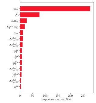
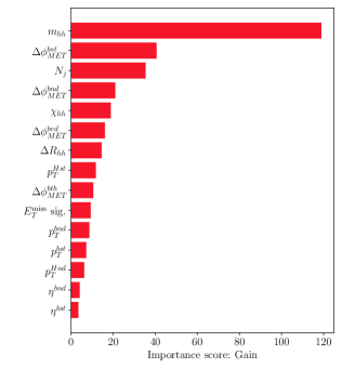
Figure 3: Importance of the features listed in Eq. (3.1) according to the gain score, for the benchmarks $750\_275\_25$ (left panel) and $750\_350\_25$ (right panel)

In Figure 3 we show the importance of the above features for the classifiers corresponding to two representative benchmarks in terms of the score gain, which gives the average improvement in accuracy obtained by adding new splits on the feature. By looking at the distributions of the features (see Appendix A) we can gain some understanding of their placing in the ranking. For example, for both benchmarks the highest ranked feature is the invariant mass $m_{hh}$, that is certainly a powerful discriminant between signal and background since it is concentrated around the intermediate scalar mass for the signal while for the backgrounds the distribution reaches it maximum at larger $m_{hh}$ values and then decreases slowly. For $750\_275\_25$ the second feature in the ranking is $N_{j}$, which also appears as the third variable in importance for $750\_350\_25$. Again, this is consistent with what is observed in the corresponding distributions: in both cases, the maximum is located at small $N_{j}$ and this allows to separate the signal from the backgrounds (except for the irreducible $Zb\bar{b}b\bar{b}$). The third most important variable for $750\_275\_25$ is $\Delta R_{hh}$, and this is consistent with the fact that the Higgs bosons tend to be boosted due to the difference in mass between the scalars $\upphi$ and $\upvarphi$, making this variable an efficient discriminator. This is not the case for $750\_350\_25$ since $\upvarphi$ is now considerably heavier, and the distributions corresponding to the signal and the different backgrounds become quite similar. In fact, we see that this variable is degraded to the 7th place for this benchmark. Finally, $\Delta\phi^{bst}_{MET}$ is the second most important feature for $750\_350\_25$ while it is in the 6th place for $750\_350\_25$, and this once again is compatible with the corresponding distributions: for $750\_350\_25$ the transverse momentum of the leading $b$-jet is more likely to lie in the same direction as the missing transverse momentum while it is in the opposite direction both for the backgrounds and the signal $750\_275\_25$; thus, it is reasonable that this feature be more useful to separate signal from background for the benchmark $750\_350\_25$.

3.2 DNN Overview and Architecture

The discussion in this section follows closely Ref. [147] and Keras documentation [148]. Deep learning provides an alternative way to approximate a mapping to predict the target variable $y$ based on the input vector of features x. In this case, the model is built in terms of units, known as neurons, which process a set of incoming signals $s_{j}$ to produce an output. Mathematically, neurons carry out two consecutive operations: first, they linearly combine the incoming signals into a preactivation variable $z$,

$$z=b+\sum_{j=1}^{n}W_{j}\cdot s_{j}\,,$$

where each signal is weighted by $W_{j}$ and biased by $b$; second, neurons fire or not according to the value of the preactivation variable $z$, and produce an outgoing signal

$$\sigma=\hat{\sigma}(z)\,.$$

The scalar-valued function $\hat{\sigma}(z)$ is called the activation function and is often taken as a rectified linear unit (ReLU) function to introduce a controllable degree of non-linearity in the model.

A set of neurons is called a layer, and stacked layers, inter-connected in such a way output signals from one layer work as the input of those neurons that belong to the subsequent layer, constitute DNN. Iteratively, DNNs are defined as

$$z_{i}^{(1)} =b_{i}^{(1)}+\sum_{j=1}^{n_{1}}W_{ij}^{(1)}\cdot s_{j}\,,$$

$$\vdots$$

$$z_{i}^{(\ell-1)} =b_{j}^{(\ell-1)}+\sum_{j=1}^{n_{\ell-1}}W_{ij}^{(\ell-1)}\cdot\hat{\sigma}\big{(}z_{j}^{(\ell-2)}\big{)}\,,$$

$$z_{i}^{(\ell)} =b_{i}^{(\ell)}+\sum_{j=1}^{n_{\ell}}W_{ij}^{(\ell)}\cdot\hat{\sigma}\big{(}z_{j}^{(\ell-1)}\big{)}\,.$$

The number of layers $\ell$ (depth), the number of neurons per layer $n_{\ell}$, and the patterns of layer connections determine the network architecture.

DNNs for binary classification tasks typically count with a single neuron in the outgoing layer, activated by a sigmoid function, instead of a ReLU, considering the DNN output is interpreted as probability. In our case, we based the architecture of the classification model on the work done in Ref. [149] for sneutrino searches, setting $500$, $500$, $250$, $100$, and $50$ neurons in five consecutive layers. To endow the network architecture with a certain level of flexibility and reduce the risk of overfitting, we set up a probability of discarding outputs of intermediate layers or dropout-rate of $21\%$.

Similarly to what was explained in the previous section, a DNN model provides a prediction $\hat{y}_{i}$ of the target variable $y_{i}$ for every data point $\textbf{x}_{i}$ in the training data set. Target and prediction are compared through an objective function, defined in terms of the training loss function $l$ as

$$\text{obj}=\sum_{i=1}^{N}l(\hat{y}_{i},y_{i})\,.$$

In this case, we took the binary cross-entropy for $l$, which is the typical choice for binary classification problems. To optimize the model, we implemented an adaptative stochastic gradient algorithm to minimize the objective function. Schematically, this kind of algorithm updates the free parameters as follows

$$\theta_{\lambda}^{(n+1)}=\theta_{\lambda}^{(n)}-\eta\frac{\partial\,\text{obj}}{\partial\theta_{\lambda}}{\bigg{|}}_{\theta=\theta^{(n)}}\,,$$

where $n$ indicates the iteration of the optimization. The learning rate $\eta$ controls the size of the step taken in the parameter space and is estimated in every iteration to improve the convergence speed. We opted for using Adam algorithm [150] with an initial learning rate value of 0.001. As in the case of XGBoost, we chose the AUC as a metric to evaluate the training performance and used the early stopping approach to avoid overtraining the model.

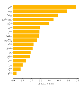
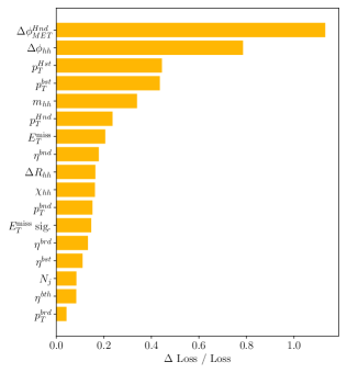
Figure 4: Ranking of the features listed in Eq. (27) according to the permutation importance score, for the benchmarks $750\_275\_25$ (left panel) and $750\_350\_25$ (right panel)

The sample used for training the DNN model includes the same events used for XGBoost split into training, validation, and test subsamples containing also $\sim$ 65%, 15%, and 20% of all the events, respectively. We tested several combinations of the kinematic variables in Section 2 as input for the training process. The best classification resulted from training the DNN model with the following set of 17 features:

$$N_{j}\,,p_{T}^{bst}\,,\eta^{bst}\,,p_{T}^{bnd}\,,\eta^{bnd}\,,p_{T}^{brd}\,,\eta^{brd}\,,\eta^{bth}\,,p_{T}^{Hst}\,,p_{T}^{Hnd}\,,E_{T}^{\text{miss}}\,,E_{T}^{\text{miss}}\text{ sign.}\,,\chi_{hh}\,,m_{hh}\,,$$

$$\Delta R_{hh}\,,\Delta\phi_{hh}\,,\text{and}\,\Delta\phi^{Hnd}_{MET}\,.$$ (27)

All features were rescaled in order to be processed by the DNN model: the method of standardization, included among Scikit-learn tools[151], gave the best discrimination results. In the subsequent discussion, we will entirely focus on the results achieved with classifiers trained using the set of kinematic variables mentioned above.

In Figure 4 we show two importance rankings of the features processed by two DNN models, trained to differentiate between benchmarks $750\_275\_25$ and $750\_350\_25$ events, respectively, from the background. Both rankings were performed using the permutation importance method, which scores every feature by breaking its relationship to the target and evaluating the predictive power deterioration of the model. Although DNN non-linear combinations of the input features used to differentiate between classification classes are not easily accessible, scrutinizing kinematic distributions related to these features helps to achieve some level of interpretability of the classification model. For example, for both benchmarks the signal distributions of $p_{T}^{bst}$ and $p_{T}^{Hst}$ peak in a different region than the corresponding background distributions, see Appendix A. This property makes them suitable to discriminate between these two classes. Another example is the case $m_{hh}$: the signal distributions are concentrated around the value of $2m_{h}$, unlikely the background which has a much flatter distribution. As expected, these three variables rank among the highest-scored features.

4 Results

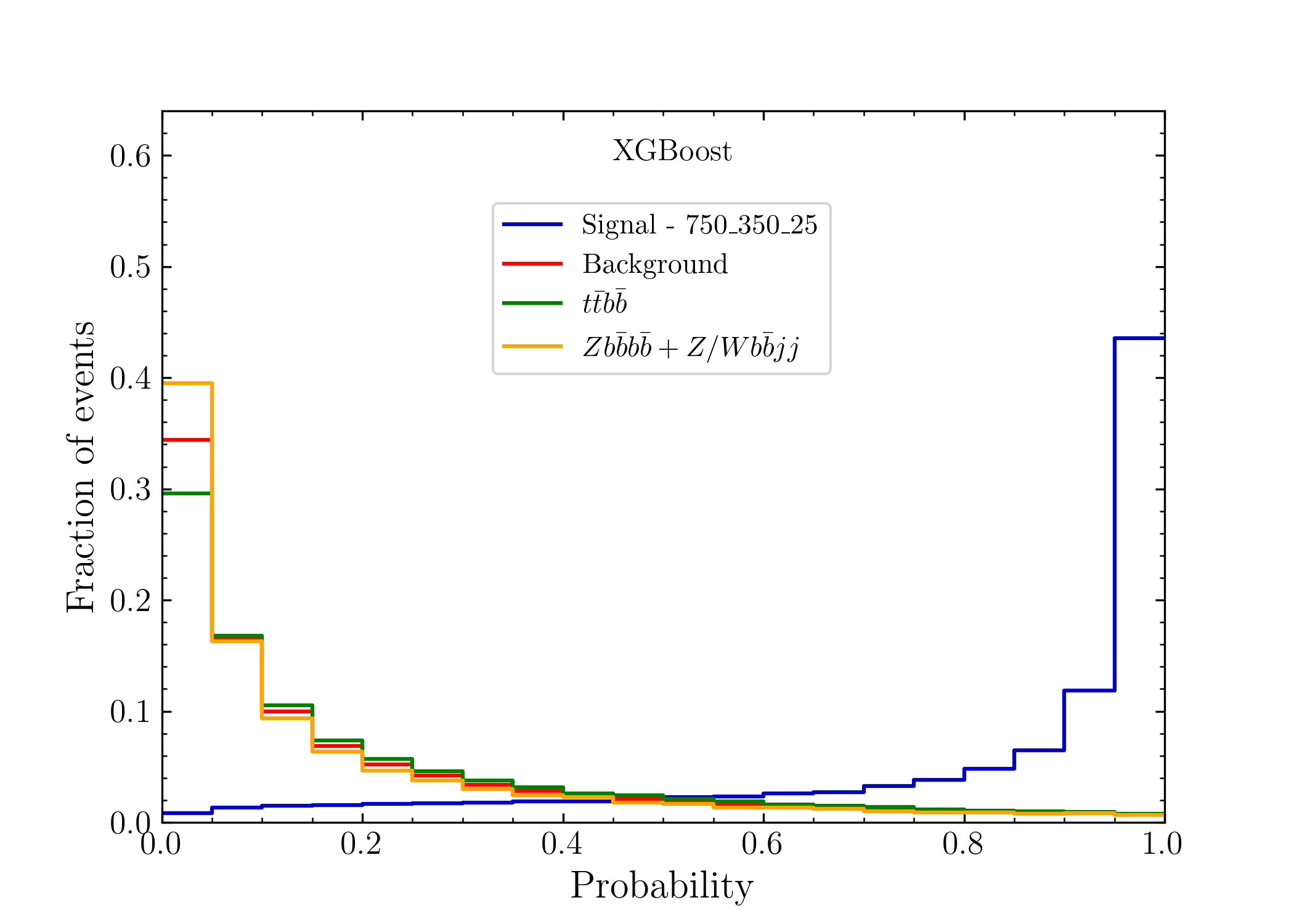
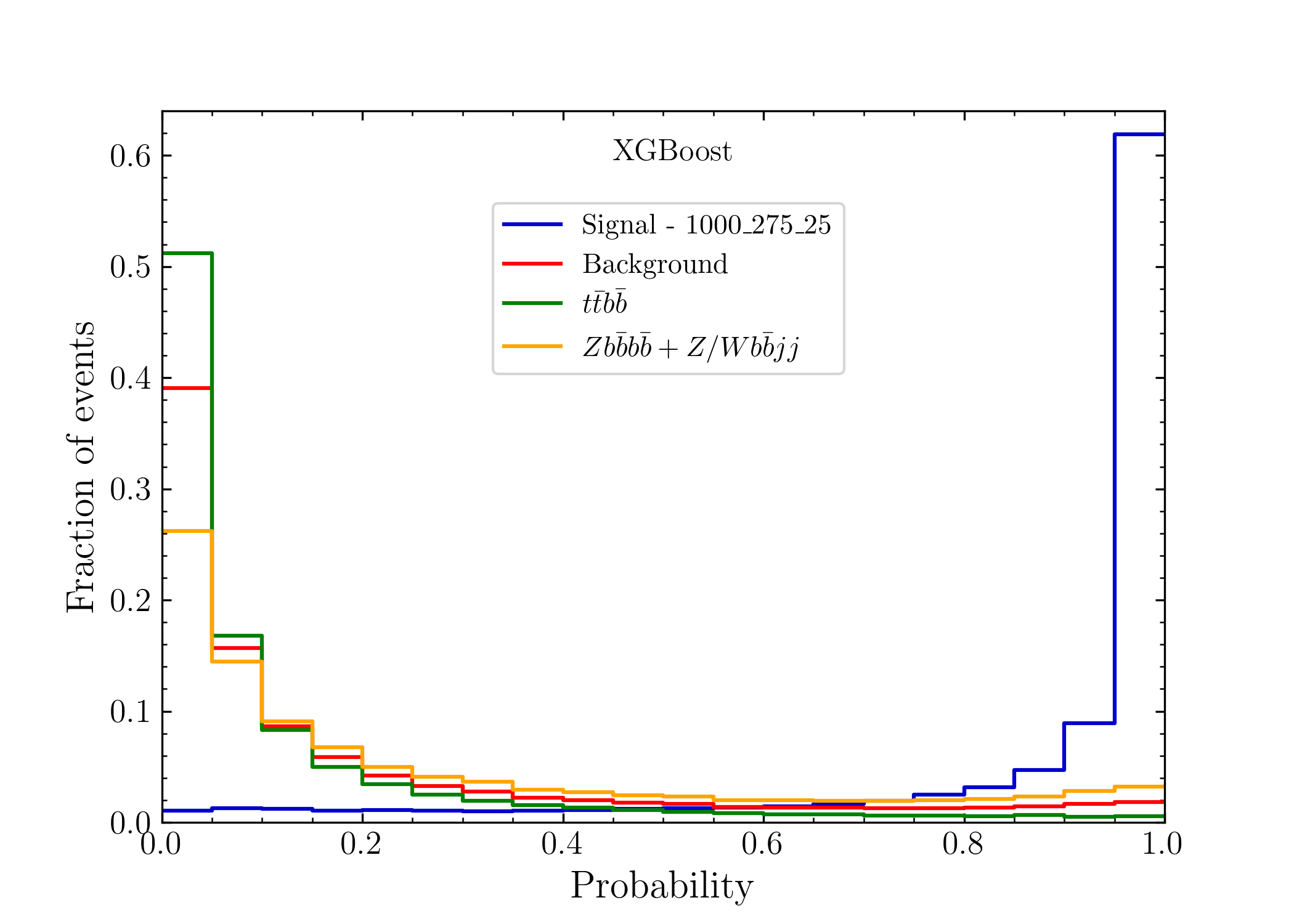
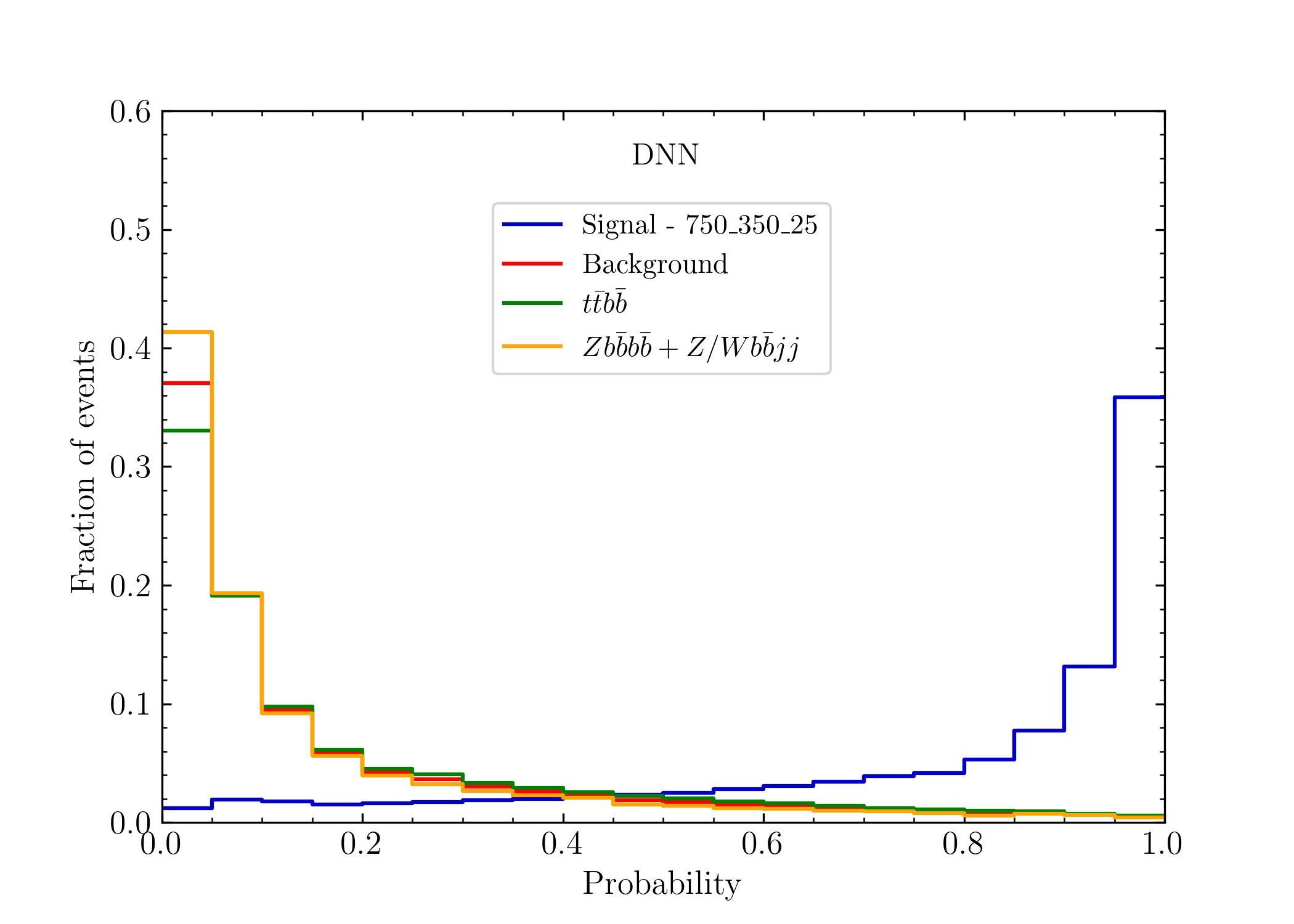
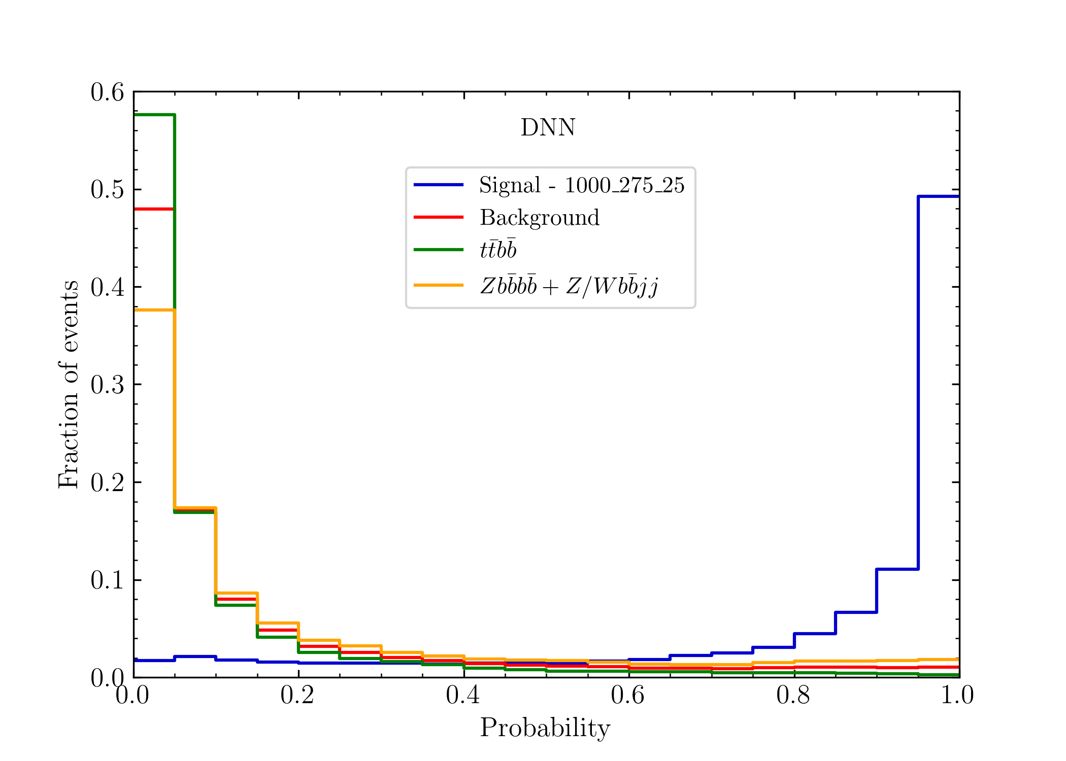
Figure 5: Probability distributions given by the output of the XGBoost and DNN classifiers for benchmarks $750\_350\_25$ and $1000\_275\_25$ along with the dominant backgrounds.

For each one of the benchmarks, we apply the corresponding XGBoost and DNN classifiers to the test samples. The output is the probability of an event being classified as a signal event. As an example, we show in Figure 5 the probability distributions for the models $750\_350\_25$ and $1000\_275\_25$. We see that both ML algorithms lead to an efficient classification of signal and background events. This is not exclusive of the two displayed benchmarks since in all the cases AUC values above 0.9 are obtained. For $1000\_275\_25$, both classifiers are better at identifying $t\bar{t}b\bar{b}$ than the rest of the background processes and this is the case for most of the benchmarks (10), the model $750\_350\_25$ is actually one of the four exceptions. Another interesting observation is that while the XGBoost classifier seems to label the signal events better, its DNN counterpart classifies the background events more efficiently. Of course, the precise values for the signal acceptance and background rejection will depend on the chosen probability threshold.

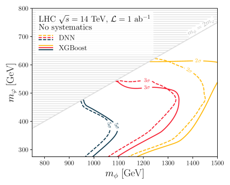
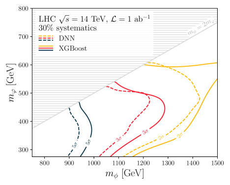
Figure 6: Significance level curves for XGBoost and DNN algorithms in the plane $[m_{\phi},m_{\upvarphi}]$ with no (left panel) and 30% (right panel) systematics. The hatched region for $m_{\phi}<2m_{\upvarphi}$ is kinematically forbbiden.

For each benchmark, the probability threshold is chosen to maximize the significance computed as [152]

$$\mathcal{S}=\sqrt{-2\left((S+B)\ln\left(\frac{B}{S+B}\right)+S\right)},$$ (28)

when potential systematic uncertainties are neglected, and using Eq. (10) otherwise. In the above expression, $S$ and $B$ are the signal and background rates after applying the cuts in Eq. (6) and the additional cut on the output of the classifiers. By interpolating the results of the 14 simulated benchmarks, we are able to plot contours of constant significance in the plane $m_{\upvarphi}$-$m_{\upphi}$. The results for XGBoost and DNNs are shown in Figure 6, where we display contours corresponding to 2$\sigma$, 3$\sigma$, and 5$\sigma$ for a luminosity of 1 ab^-1. Since the performance of the classifiers of each benchmark are quite similar, with AUC above 0.9 in all the cases, the shape of the contours is mostly driven by the effective cross section. In fact, by comparing with Figure 2, it is easy to recognize the behavior of the effective cross section in the contours displayed in Figure 6.

With systematic uncertainties neglected, we see that for $m_{\upphi}$ below $\sim 950$ GeV discovery-level significances are reached for all the kinematically allowed intermediate scalar $\upvarphi$ masses. Moreover, for $m_{\upvarphi}$ around 380 GeV, the discovery region extends in the $m_{\upphi}$-range up to $\sim 1090$ GeV with XGBoost and $\sim 1060$ GeV with DNNs. Evidence-level significances can be obtained for $\upphi$ as heavy as $\sim 1340$ GeV providing the intermediate scalar $\upvarphi$ mass is $\sim 480$ GeV. In general, when the impact of the systematic uncertainties is not included, the results of ${\tt XGBoost}$ tend to slightly improve those of the DNNs.

In the right panel of Figure 6 we show how the results are degraded when 30% of systematic uncertainties on the total background are included. Since the expression in Eq. (10) penalizes the presence of background, now the thresholds optimizing the significance shift to increase the background rejection at the cost of decreasing the signal acceptance. This can be directly verified by comparing the acceptances of signal and backgrounds obtained before and after including the systematic uncertainties (see Tables 4-7 in the Appendix B). Discovery-level significances are obtained for all the kinematically allowed range of $m_{\upvarphi}$ for $m_{\upphi}<900$ GeV, and the discovery region reaches heavy scalar masses of $\sim 990$ GeV for $m_{\upvarphi}$ around 370 GeV. The evidence level can be reached now for $m_{\upphi}$ up to $\sim 1290$ GeV when $m_{\upvarphi}\sim 450$ GeV. Again, the XGBoost classifiers appear to provide better prospects. Moreover, the improvement is more significant when the impact of systematic uncertainties is included. This is consistent with the acceptances displayed in Tables  4-7 of Appendix B, where we see that DNN classifiers keep more signal events than XGBoost classifiers, but at the expense of rejecting considerably less background events. The improvement in signal acceptance is not enough to compensate for the worse background rejection, which is strongly penalized by Eq. (10). The fact that after applying the probability threshold the DNN classifiers keep more background events is not in conflict with the observation made before about their better discrimination of the background. Since the background is better classified than the signal, a threshold that keeps as many signal events as possible is preferred, even when this means keeping more background events. In contrast, the XGBoost classifiers are better at classifying the signal, and then a threshold that rejects as many background events as possible is optimal, even when it leads to a smaller signal acceptance.

The results in Figure 6 show a significant improvement with respect to the prospects achieved by using a traditional cut and count analysis. In particular, when a 15% of systematics uncertainties is considered, significances above the evidence level are obtained for 7 (XGBoost) and 6 (DNN) out of the 14 simulated benchmarks, while with the analysis based on rectangular cuts only two benchmarks, 750_350_25 and 1000_275_25, lead to significances above $3\sigma$. As pointed out in Section 2, the significances reached with the cut and count analysis for these benchmarks are $3.77$ and $3.48$, respectively. The performance of the ML algorithms is significantly better, giving rise to 11.75 (XGBoost) and 10.67 (DNN) for 750_350_25, and 4.51 (XGBoost) and 3.78 (DNN) for 1000_275_25. Moreover, if the potential systematic uncertainties on the total background are increased to 30% , the significances obtained with the cut and count analysis drop below the evidence level, while this is not the case when the ML classifiers are used.

5 Conclusions

In this paper we study the performance of two types of modern machine-learning algorithms, namely XGBoost and deep neural networks, on the LHC signature consisting of 4 $b$-jets and large missing transverse energy, comparing it against traditional analyses based on rectangular cuts. We work within the context of simplified models that generically parameterize a large class of models with heavy scalars and dark matter candidates, consisting of an extended scalar sector with three real scalar particles: the heaviest of these new scalars, $\upphi$, produced via gluon fusion at the LHC, predominantly decays to a pair of intermediate scalars $\upvarphi$, which interact with the visible sector only through its coupling with the SM Higgs boson $h$; the third and lightest scalar $\chi$ is the DM candidate within this effective field theory framework. Therefore, the proposed LHC signature comes from the resonant production of $\upphi$, that decays into a pair of $\upvarphi$. One of these $\upvarphi$ decays in turn into two $h$, decaying both into $b$-quarks pairs, while the other $\upvarphi$ decays invisibly into a pair of $\chi$. The dominant irreducible backgrounds are $Z+b\bar{b}b\bar{b}$ and $t\bar{t}+b\bar{b}$; the main reducible backgrounds correspond to $V$+jets (concretely $Z/W+b\bar{b}+jj$), while QCD multijet can be safely ignored since it does not provide a true source of $E_{T}^{\text{miss}}$.

We scan $m_{\upphi}$ and $m_{\upvarphi}$ in the ranges [750, 1500] GeV and [275, $m_{\upphi}/2$] GeV, respectively, and consider 15 low-level and 18 high-level kinematic features with which we feed the ML algorithms. The discriminating power of these detector-level features varies by benchmark, but we have found that in general the most important are those related to the $hh$ system and $E_{T}^{\text{miss}}$, along with the $p_{T}$ of the most energetic jets.

Our performance comparison between both ML algorithms is based on the maximum significance reached for an LHC center-of-mass energy of 14 TeV and a total integrated luminosity of 1 ab^-1. Both algorithms present very similar performances and a significant improvement with respect to the prospects achieved by using a traditional cut and count analysis. In most of the parameter space, the results of ${\tt XGBoost}$ tend to slightly improve those of the DNNs due to the signal acceptance and background rejection interplay in each case when the significance is maximized. If a 15% of systematics uncertainties on the background is considered, significances larger than the evidence level are obtained for a large part of the 14 simulated benchmarks, while with the cut-based analysis only two benchmarks, 750_350_25 and 1000_275_25, provide significances above $3\sigma$ ($3.77$ and $3.48$, respectively). The signal significances from XGBoost and DNN are much better: 11.75 (XGBoost) and 10.67 (DNN) for 750_350_25, and 4.51 (XGBoost) and 3.78 (DNN) for 1000_275_25. In addition, if a 30% systematic uncertainty on the total background is considered, the significances obtained with the traditional analysis drop below the evidence level, whilst the ML classifiers still provide values up to the discovery level.

As a general conclusion, we consider that our phenomenological analysis shows that the proposed LHC signature deserves the development of dedicated searches by the experimental collaborations, for which modern ML algorithms such as XGBoost and DNN would play a crucial role.

Appendices

Appendix A Relevant Kinematic Distributions

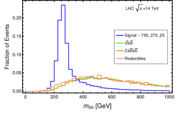
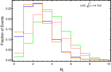
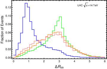
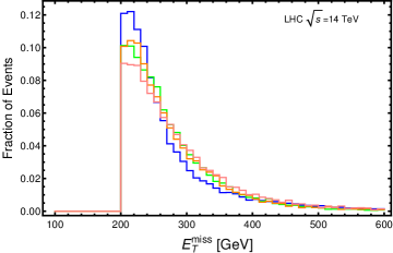
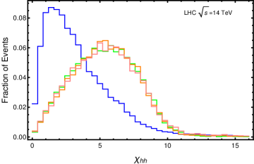
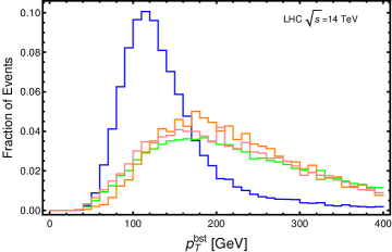
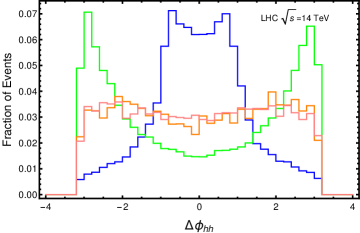
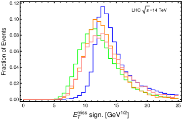
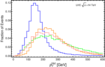
Figure 7: Distributions of some of the kinematic variables used as inputs during the training of XGBoost and DNNs classifiers for the benchmark 750_275_25.

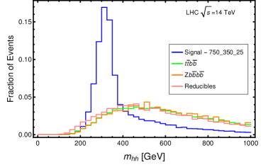
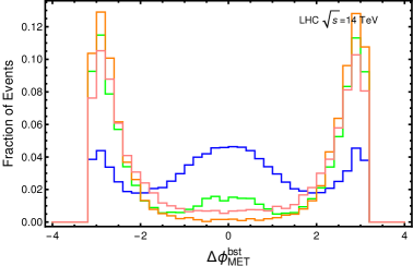
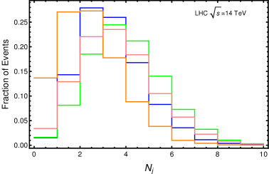
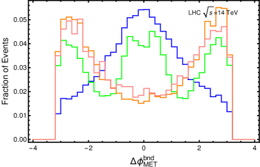
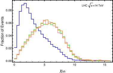
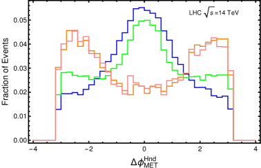
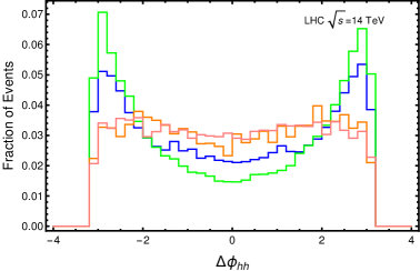
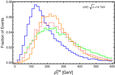
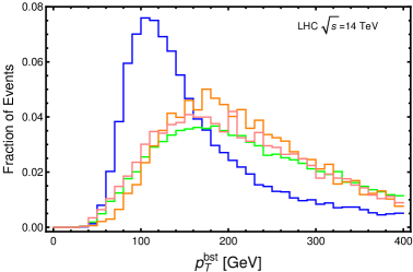
Figure 8: Distributions of some of the kinematic variables used as inputs during the training of XGBoost and DNNs classifiers for the benchmark 750_350_25.

As an illustration, the distributions of some of the most relevant features presented in Section 3 for the benchmarks 750_275_25 and 750_350_25 are collected in Figure 7 and Figure 8, respectively. These kinematic variables correspond to detector-level events in the signal region defined by Eq. (6). Some of them exhibit an explicit signal-background separation and have been used in the cut and count analysis presented in Section 2. Also, these variables are part of the inputs used to train the ML classifiers. Their importance in the training procedure is shown in Sections 3.1 and 3.2 for XGBoost and DNNs, respectively.

Appendix B Tables of Acceptance

We provide tables with the acceptance of the signal and the different backgrounds included in this study. In ML jargon these correspond to the true positive rate for the signal and the false positive rate for the backgrounds. Each row is associated to a classifier trained for the benchmark $m_{\upphi}\_m_{\upvarphi}$ and to the probability threshold that maximizes the significance.

$m_{\upphi}$	$m_{\upvarphi}$	Signal	$Z|_{\rm inv}b\bar{b}jj$	$W^{\pm}|_{\rm semilep}b\bar{b}jj$	$t\bar{t}|_{\rm semilep}b\bar{b}$	$t\bar{t}|_{\rm semitau}b\bar{b}$	$Z|_{\rm inv}b\bar{b}b\bar{b}$
750	275	0.4047	0.0139	0.0135	0.0047	0.0053	0.0162
750	350	0.4172	0.0066	0.0075	0.0088	0.0078	0.0010
1000	275	0.3136	0.0054	0.0054	0.0005	0.0008	0.0039
1000	375	0.3551	0.0126	0.0129	0.0045	0.0054	0.0159
1000	475	0.2485	0.0007	0.0010	0.0014	0.0014	0.0001
1250	275	0.2141	0.0015	0.0012	0.0001	0.0002	0.0008
1250	375	0.3032	0.0033	0.0030	0.0004	0.0006	0.0021
1250	475	0.2384	0.0019	0.0020	0.0004	0.0003	0.0018
1250	600	0.2485	0.0006	0.0009	0.0005	0.0004	0.0001
1500	275	0.2537	0.0019	0.0021	0.0001	0.0002	0.0011
1500	375	0.2786	0.0013	0.0013	0.0001	0.0002	0.0007
1500	475	0.2458	0.0009	0.0009	0.0001	0.0001	0.0004
1500	600	0.2450	0.0009	0.0010	0.0001	0.0001	0.0008
1500	725	0.2560	0.0003	0.0005	0.0004	0.0002	0.0001

Table 4: Acceptances for DNN classifiers after applying a probability threshold that maximizes the significance without including systematic uncertainties.

$m_{\upphi}$	$m_{\upvarphi}$	Signal	$Z|_{\rm inv}b\bar{b}jj$	$W^{\pm}|_{\rm semilep}b\bar{b}jj$	$t\bar{t}|_{\rm semilep}b\bar{b}$	$t\bar{t}|_{\rm semitau}b\bar{b}$	$Z|_{\rm inv}b\bar{b}b\bar{b}$
750	275	0.3805	0.0093	0.0084	0.0029	0.0034	0.0126
750	350	0.4147	0.0065	0.0071	0.0067	0.0059	0.0007
1000	275	0.3265	0.0036	0.0038	0.0004	0.0003	0.0017
1000	375	0.3134	0.0077	0.0076	0.0018	0.0032	0.0086
1000	475	0.1061	8.0902	$<10^{-4}$	0.0001	0.0001	$<10^{-4}$
1250	275	0.1951	0.0008	0.0010	0.0001	0.0001	0.0007
1250	375	0.2561	0.0015	0.0017	$<10^{-4}$	0.0001	0.0012
1250	475	0.2735	0.0024	0.0029	0.0003	0.0004	0.0035
1250	600	0.2995	0.0009	0.0017	0.0009	0.0009	0.0002
1500	275	0.1914	0.0009	0.0010	$<10^{-4}$	$<10^{-4}$	0.0010
1500	375	0.2627	0.0009	0.0009	0.0001	$<10^{-4}$	0.0007
1500	475	0.2324	0.0007	0.0009	$<10^{-4}$	$<10^{-4}$	0.0002
1500	600	0.0855	$<10^{-4}$	0.0001	$<10^{-4}$	$<10^{-4}$	$<10^{-4}$
1500	725	0.2297	0.0002	0.0006	0.0001	0.0002	0.0002

Table 5: Acceptances for XGBoost classifiers after applying a probability threshold that maximizes the significance without including systematic uncertainties.

$m_{\upphi}$	$m_{\upvarphi}$	Signal	$Z|_{\rm inv}b\bar{b}jj$	$W^{\pm}|_{\rm semilep}b\bar{b}jj$	$t\bar{t}|_{\rm semilep}b\bar{b}$	$t\bar{t}|_{\rm semitau}b\bar{b}$	$Z|_{\rm inv}b\bar{b}b\bar{b}$
750	275	0.1736	0.0024	0.0021	0.0009	0.0007	0.0031
750	350	0.1528	0.0007	0.0006	0.0008	0.0008	$<10^{-4}$
1000	275	0.1999	0.0021	0.0021	0.0001	0.0003	0.0012
1000	375	0.1411	0.0021	0.0021	0.0007	0.0008	0.0022
1000	475	0.1706	0.0003	0.0004	0.0006	0.0007	$<10^{-4}$
1250	275	0.1632	0.0008	0.0006	$<10^{-4}$	0.0001	0.0004
1250	375	0.1990	0.0013	0.0013	0.0002	0.0003	0.0008
1250	475	0.1678	0.0008	0.0008	0.0003	0.0001	0.0007
1250	600	0.2063	0.0004	0.0006	0.0004	0.0003	0.0001
1500	275	0.2150	0.0014	0.0014	0.0001	0.0001	0.0007
1500	375	0.2410	0.0010	0.0010	0.0001	0.0001	0.0004
1500	475	0.2243	0.0007	0.0007	0.0001	0.0001	0.0003
1500	600	0.2134	0.0006	0.0008	0.0001	0.0001	0.0005
1500	725	0.2296	0.0002	0.0004	0.0003	0.0002	$<10^{-4}$

Table 6: Acceptances for DNN classifiers after applying a probability threshold that maximizes the significance including 30% of systematic uncertainties in the total background yield.

$m_{\upphi}$	$m_{\upvarphi}$	Signal	$Z|_{\rm inv}b\bar{b}jj$	$W^{\pm}|_{\rm semilep}b\bar{b}jj$	$t\bar{t}|_{\rm semilep}b\bar{b}$	$t\bar{t}|_{\rm semitau}b\bar{b}$	$Z|_{\rm inv}b\bar{b}b\bar{b}$
750	275	0.1722	0.0015	0.0009	0.0004	0.0003	0.0015
750	350	0.1650	0.0006	0.0005	0.0005	0.0003	$<10^{-4}$
1000	275	0.2371	0.0017	0.0016	0.0002	0.0002	0.0012
1000	375	0.1391	0.0014	0.0014	0.0002	0.0005	0.0020
1000	475	0.1061	8.0902	$<10^{-4}$	0.0001	0.0001	$<10^{-4}$
1250	275	0.0749	0.0001	0.0001	$<10^{-4}$	$<10^{-4}$	$<10^{-4}$
1250	375	0.2561	0.0015	0.0017	$<10^{-4}$	0.0001	0.0012
1250	475	0.1180	0.0003	0.0006	$<10^{-4}$	$<10^{-4}$	0.0005
1250	600	0.1983	0.0004	0.0007	0.0002	0.0004	0.0002
1500	275	0.1914	0.0009	0.0010	$<10^{-4}$	$<10^{-4}$	0.0010
1500	375	0.1259	0.0009	0.0002	$<10^{-4}$	$<10^{-4}$	$<10^{-4}$
1500	475	0.2324	0.0007	0.0009	$<10^{-4}$	$<10^{-4}$	0.0002
1500	600	0.0855	$<10^{-4}$	0.0001	$<10^{-4}$	$<10^{-4}$	$<10^{-4}$
1500	725	0.2298	0.0002	0.0006	0.0001	0.0002	0.0002

Table 7: Acceptances for XGBoost classifiers after applying a probability threshold that maximizes the significance including 30% of systematic uncertainties in the total background yield.

References

- [1] A. J. Larkoski, I. Moult and B. Nachman, Jet Substructure at the Large Hadron Collider: A Review of Recent Advances in Theory and Machine Learning, Phys. Rept. 841 (2020) 1 [1709.04464].
- [2] D. Guest, K. Cranmer and D. Whiteson, Deep Learning and its Application to LHC Physics, Ann. Rev. Nucl. Part. Sci. 68 (2018) 161 [1806.11484].
- [3] K. Albertsson et al., Machine Learning in High Energy Physics Community White Paper, J. Phys. Conf. Ser. 1085 (2018) 022008 [1807.02876].
- [4] A. Radovic, M. Williams, D. Rousseau, M. Kagan, D. Bonacorsi, A. Himmel et al., Machine learning at the energy and intensity frontiers of particle physics, Nature 560 (2018) 41.
- [5] G. Carleo, I. Cirac, K. Cranmer, L. Daudet, M. Schuld, N. Tishby et al., Machine learning and the physical sciences, Rev. Mod. Phys. 91 (2019) 045002 [1903.10563].
- [6] D. Bourilkov, Machine and Deep Learning Applications in Particle Physics, Int. J. Mod. Phys. A 34 (2020) 1930019 [1912.08245].
- [7] M. Feickert and B. Nachman, A Living Review of Machine Learning for Particle Physics, 2102.02770.
- [8] M. D. Schwartz, Modern Machine Learning and Particle Physics, 2103.12226.
- [9] G. Karagiorgi, G. Kasieczka, S. Kravitz, B. Nachman and D. Shih, Machine Learning in the Search for New Fundamental Physics, 2112.03769.
- [10] P. Shanahan et al., Snowmass 2021 Computational Frontier CompF03 Topical Group Report: Machine Learning, 2209.07559.
- [11] T. Plehn, A. Butter, B. Dillon and C. Krause, Modern Machine Learning for LHC Physicists, 2211.01421.
- [12] CMS collaboration, Search for Supersymmetry in Events with Opposite-Sign Dileptons and Missing Transverse Energy Using an Artificial Neural Network, Phys. Rev. D 87 (2013) 072001 [1301.0916].
- [13] ATLAS collaboration, Search for invisible particles produced in association with single-top-quarks in proton-proton collisions at = 8 TeV with the ATLAS detector, Eur. Phys. J. C 75 (2015) 79 [1410.5404].
- [14] ATLAS collaboration, Search for the electroweak production of supersymmetric particles in =8 TeV collisions with the ATLAS detector, Phys. Rev. D 93 (2016) 052002 [1509.07152].
- [15] CMS collaboration, Search for resonant and nonresonant Higgs boson pair production in the final state in proton-proton collisions at TeV, JHEP 01 (2018) 054 [1708.04188].
- [16] CMS collaboration, Identification of heavy-flavour jets with the CMS detector in pp collisions at 13 TeV, JINST 13 (2018) P05011 [1712.07158].
- [17] CMS collaboration, Search for production in the decay channel with leptonic decays in proton-proton collisions at TeV, JHEP 03 (2019) 026 [1804.03682].
- [18] ATLAS collaboration, Search for pair production of heavy vector-like quarks decaying into high- bosons and top quarks in the lepton-plus-jets final state in collisions at TeV with the ATLAS detector, JHEP 08 (2018) 048 [1806.01762].
- [19] ATLAS collaboration, Searches for scalar leptoquarks and differential cross-section measurements in dilepton-dijet events in proton-proton collisions at a centre-of-mass energy of = 13 TeV with the ATLAS experiment, Eur. Phys. J. C 79 (2019) 733 [1902.00377].
- [20] ATLAS collaboration, Search for long-lived neutral particles in collisions at = 13 TeV that decay into displaced hadronic jets in the ATLAS calorimeter, Eur. Phys. J. C 79 (2019) 481 [1902.03094].
- [21] CMS collaboration, Search for direct pair production of supersymmetric partners to the lepton in proton-proton collisions at 13 TeV, Eur. Phys. J. C 80 (2020) 189 [1907.13179].
- [22] CMS collaboration, Search for a charged Higgs boson decaying into top and bottom quarks in events with electrons or muons in proton-proton collisions at = 13 TeV, JHEP 01 (2020) 096 [1908.09206].
- [23] ATLAS collaboration, Search for light long-lived neutral particles produced in collisions at 13 TeV and decaying into collimated leptons or light hadrons with the ATLAS detector, Eur. Phys. J. C 80 (2020) 450 [1909.01246].
- [24] CMS collaboration, A deep neural network to search for new long-lived particles decaying to jets, Mach. Learn. Sci. Tech. 1 (2020) 035012 [1912.12238].
- [25] CMS collaboration, Measurements of Production and the CP Structure of the Yukawa Interaction between the Higgs Boson and Top Quark in the Diphoton Decay Channel, Phys. Rev. Lett. 125 (2020) 061801 [2003.10866].
- [26] CMS collaboration, Identification of heavy, energetic, hadronically decaying particles using machine-learning techniques, JINST 15 (2020) P06005 [2004.08262].
- [27] ATLAS collaboration, Search for resonances in fully hadronic final states in collisions at = 13 TeV with the ATLAS detector, JHEP 10 (2020) 061 [2005.05138].
- [28] ATLAS collaboration, Reconstruction and identification of boosted di- systems in a search for Higgs boson pairs using 13 TeV proton-proton collision data in ATLAS, JHEP 11 (2020) 163 [2007.14811].
- [29] CMS collaboration, Search for nonresonant Higgs boson pair production in final states with two bottom quarks and two photons in proton-proton collisions at = 13 TeV, JHEP 03 (2021) 257 [2011.12373].
- [30] CMS collaboration, Search for top squark production in fully-hadronic final states in proton-proton collisions at 13 TeV, Phys. Rev. D 104 (2021) 052001 [2103.01290].
- [31] ATLAS collaboration, Search for R-parity-violating supersymmetry in a final state containing leptons and many jets with the ATLAS experiment using proton–proton collision data, Eur. Phys. J. C 81 (2021) 1023 [2106.09609].
- [32] ATLAS collaboration, Search for neutral long-lived particles in collisions at = 13 TeV that decay into displaced hadronic jets in the ATLAS calorimeter, JHEP 06 (2022) 005 [2203.01009].
- [33] CMS collaboration, Reconstruction of decays to merged photons using end-to-end deep learning with domain continuation in the CMS detector, Phys. Rev. D 108 (2023) 052002 [2204.12313].
- [34] ATLAS collaboration, Search for light long-lived neutral particles that decay to collimated pairs of leptons or light hadrons in pp collisions at = 13 TeV with the ATLAS detector, JHEP 06 (2023) 153 [2206.12181].
- [35] ATLAS collaboration, Search for resonant WZ production in the fully leptonic final state in proton–proton collisions at TeV with the ATLAS detector, Eur. Phys. J. C 83 (2023) 633 [2207.03925].
- [36] CMS collaboration, Search for violation in ttH and tH production in multilepton channels in proton-proton collisions at = 13 TeV, JHEP 07 (2023) 092 [2208.02686].
- [37] CMS collaboration, Search for new physics using effective field theory in 13 TeV pp collision events that contain a top quark pair and a boosted Z or Higgs boson, Phys. Rev. D 108 (2023) 032008 [2208.12837].
- [38] CMS collaboration, Search for new heavy resonances decaying to WW, WZ, ZZ, WH, or ZH boson pairs in the all-jets final state in proton-proton collisions at = 13 TeV, Phys. Lett. B 844 (2023) 137813 [2210.00043].
- [39] CMS collaboration, Search for supersymmetry in final states with a single electron or muon using angular correlations and heavy-object identification in proton-proton collisions at = 13 TeV, JHEP 09 (2023) 149 [2211.08476].
- [40] CMS collaboration, Search for long-lived particles using out-of-time trackless jets in proton-proton collisions at = 13 TeV, JHEP 07 (2023) 210 [2212.06695].
- [41] ATLAS collaboration, Search for nonresonant pair production of Higgs bosons in the bb¯bb¯ final state in pp collisions at s=13 TeV with the ATLAS detector, Phys. Rev. D 108 (2023) 052003 [2301.03212].
- [42] CMS collaboration, Search for top squarks in the four-body decay mode with single lepton final states in proton-proton collisions at = 13 TeV, JHEP 06 (2023) 060 [2301.08096].
- [43] CMS collaboration, Search for a vector-like quark T′ tH via the diphoton decay mode of the Higgs boson in proton-proton collisions at = 13 TeV, JHEP 09 (2023) 057 [2302.12802].
- [44] CMS collaboration, Search for the lepton-flavor violating decay of the Higgs boson and additional Higgs bosons in the e final state in proton-proton collisions at = 13 TeV, Phys. Rev. D 108 (2023) 072004 [2305.18106].
- [45] ATLAS collaboration, Anomaly detection search for new resonances decaying into a Higgs boson and a generic new particle in hadronic final states using TeV collisions with the ATLAS detector, Phys. Rev. D 108 (2023) 052009 [2306.03637].
- [46] ATLAS collaboration, Search for new phenomena in two-body invariant mass distributions using unsupervised machine learning for anomaly detection at TeV with the ATLAS detector, 2307.01612.
- [47] CMS collaboration, Search for scalar leptoquarks produced in lepton-quark collisions and coupled to leptons, 2308.06143.
- [48] CMS collaboration, Search for supersymmetry in final states with disappearing tracks in proton-proton collisions at = 13 TeV, 2309.16823.
- [49] CMS collaboration, Search for direct production of GeV-scale resonances decaying to a pair of muons in proton-proton collisions at = 13 TeV, 2309.16003.
- [50] CMS collaboration, Search for a new resonance decaying into two spin-0 bosons in a final state with two photons and two bottom quarks in proton-proton collisions at = 13 TeV, 2310.01643.
- [51] CMS collaboration, Search for dark matter particles in W+W- events with transverse momentum imbalance in proton-proton collisions at = 13 TeV, 2310.12229.
- [52] ATLAS collaboration, Studies of new Higgs boson interactions through nonresonant production in the final state in collisions at TeV with the ATLAS detector, 2310.12301.
- [53] CMS collaboration, Search for an exotic decay of the Higgs boson into a Z boson and a pseudoscalar particle in proton-proton collisions at = 13 TeV, 2311.00130.
- [54] CMS, TOTEM collaboration, Search for high-mass exclusive diphoton production with tagged protons in proton-proton collisions at = 13 TeV, 2311.02725.
- [55] CMS collaboration, Search for new Higgs bosons via same-sign top quark pair production in association with a jet in proton-proton collisions at = 13 TeV, 2311.03261.
- [56] ATLAS collaboration, Observation of a new particle in the search for the Standard Model Higgs boson with the ATLAS detector at the LHC, Phys. Lett. B 716 (2012) 1 [1207.7214].
- [57] CMS collaboration, Observation of a New Boson at a Mass of 125 GeV with the CMS Experiment at the LHC, Phys. Lett. B 716 (2012) 30 [1207.7235].
- [58] ATLAS, CMS collaboration, Combined Measurement of the Higgs Boson Mass in Collisions at and 8 TeV with the ATLAS and CMS Experiments, Phys. Rev. Lett. 114 (2015) 191803 [1503.07589].
- [59] ATLAS, CMS collaboration, Measurements of the Higgs boson production and decay rates and constraints on its couplings from a combined ATLAS and CMS analysis of the LHC pp collision data at and 8 TeV, JHEP 08 (2016) 045 [1606.02266].
- [60] ATLAS collaboration, Search for heavy resonances decaying into in the final state in collisions at TeV with the ATLAS detector, Eur. Phys. J. C 78 (2018) 24 [1710.01123].
- [61] ATLAS collaboration, Search for charged Higgs bosons decaying via in the +jets and +lepton final states with 36 fb-1 of collision data recorded at TeV with the ATLAS experiment, JHEP 09 (2018) 139 [1807.07915].
- [62] ATLAS collaboration, Search for heavy neutral Higgs bosons produced in association with -quarks and decaying into -quarks at TeV with the ATLAS detector, Phys. Rev. D 102 (2020) 032004 [1907.02749].
- [63] CMS collaboration, Search for heavy Higgs bosons decaying to a top quark pair in proton-proton collisions at 13 TeV, JHEP 04 (2020) 171 [1908.01115].
- [64] ATLAS collaboration, Search for heavy Higgs bosons decaying into two tau leptons with the ATLAS detector using collisions at TeV, Phys. Rev. Lett. 125 (2020) 051801 [2002.12223].
- [65] CMS collaboration, Measurement of the -violating phase in the B J(1020) K+K- channel in proton-proton collisions at 13 TeV, Phys. Lett. B 816 (2021) 136188 [2007.02434].
- [66] ATLAS collaboration, Search for heavy resonances decaying into a pair of Z bosons in the and final states using 139 of proton–proton collisions at TeV with the ATLAS detector, Eur. Phys. J. C 81 (2021) 332 [2009.14791].
- [67] ATLAS collaboration, Search for charged Higgs bosons decaying into a top quark and a bottom quark at = 13 TeV with the ATLAS detector, JHEP 06 (2021) 145 [2102.10076].
- [68] CMS collaboration, Search for new particles in events with energetic jets and large missing transverse momentum in proton-proton collisions at = 13 TeV, JHEP 11 (2021) 153 [2107.13021].
- [69] CMS collaboration, Probing effective field theory operators in the associated production of top quarks with a Z boson in multilepton final states at = 13 TeV, JHEP 12 (2021) 083 [2107.13896].
- [70] CMS collaboration, Search for high mass resonances decaying into in the dileptonic final state with of proton-proton collisions at , CMS-PAS-HIG-20-016 (2022) .
- [71] CMS collaboration, Constraints on anomalous Higgs boson couplings to vector bosons and fermions from the production of Higgs bosons using the final state, Phys. Rev. D 108 (2023) 032013 [2205.05120].
- [72] CMS collaboration, Search for Higgs boson pairs decaying to WW*WW*, WW*, and in proton-proton collisions at = 13 TeV, JHEP 07 (2023) 095 [2206.10268].
- [73] CMS collaboration, Search for a new resonance decaying to two scalars in the final state with two bottom quarks and two photons in proton-proton collisions at , CMS-PAS-HIG-21-011 (2022) .
- [74] ATLAS collaboration, Search for heavy resonances decaying into a or boson and a Higgs boson in final states with leptons and -jets in fb-1 of collisions at TeV with the ATLAS detector, JHEP 06 (2023) 016 [2207.00230].
- [75] CMS collaboration, Search for a charged Higgs boson decaying into a heavy neutral Higgs boson and a W boson in proton-proton collisions at = 13 TeV, JHEP 09 (2023) 032 [2207.01046].
- [76] CMS collaboration, Searches for additional Higgs bosons and for vector leptoquarks in final states in proton-proton collisions at = 13 TeV, JHEP 07 (2023) 073 [2208.02717].
- [77] ATLAS collaboration, Search for Higgs boson pair production in association with a vector boson in pp collisions at with the ATLAS detector, Eur. Phys. J. C 83 (2023) 519 [2210.05415].
- [78] ATLAS collaboration, Search for production in the multilepton final state in proton–proton collisions at = 13 TeV with the ATLAS detector, JHEP 07 (2023) 203 [2211.01136].
- [79] ATLAS collaboration, A search for heavy Higgs bosons decaying into vector bosons in same-sign two-lepton final states in pp collisions at = 13 TeV with the ATLAS detector, JHEP 07 (2023) 200 [2211.02617].
- [80] ATLAS collaboration, Search for a new heavy scalar particle decaying into a Higgs boson and a new scalar singlet in final states with one or two light leptons and a pair of -leptons with the ATLAS detector, JHEP 10 (2023) 009 [2307.11120].
- [81] ATLAS collaboration, Search for heavy Higgs bosons with flavour-violating couplings in multi-lepton plus -jets final states in collisions at 13 TeV with the ATLAS detector, 2307.14759.
- [82] ATLAS collaboration, Search for the Z decay mode of new high-mass resonances in pp collisions at s=13 TeV with the ATLAS detector, Phys. Lett. B 848 (2024) 138394 [2309.04364].
- [83] ATLAS collaboration, Search for a CP-odd Higgs boson decaying into a heavy CP-even Higgs boson and a boson in the and final states using 140 fb-1 of data collected with the ATLAS detector, 2311.04033.
- [84] ATLAS collaboration, Combination of searches for resonant Higgs boson pair production using collisions at TeV with the ATLAS detector, 2311.15956.
- [85] V. Silveira and A. Zee, SCALAR PHANTOMS, Phys. Lett. B 161 (1985) 136.
- [86] R. M. Schabinger and J. D. Wells, A Minimal spontaneously broken hidden sector and its impact on Higgs boson physics at the large hadron collider, Phys. Rev. D 72 (2005) 093007 [hep-ph/0509209].
- [87] B. Patt and F. Wilczek, Higgs-field portal into hidden sectors, hep-ph/0605188.
- [88] D. O’Connell, M. J. Ramsey-Musolf and M. B. Wise, Minimal Extension of the Standard Model Scalar Sector, Phys. Rev. D 75 (2007) 037701 [hep-ph/0611014].
- [89] L. Lopez Honorez, E. Nezri, J. F. Oliver and M. H. G. Tytgat, The Inert Doublet Model: An Archetype for Dark Matter, JCAP 02 (2007) 028 [hep-ph/0612275].
- [90] J. March-Russell, S. M. West, D. Cumberbatch and D. Hooper, Heavy Dark Matter Through the Higgs Portal, JHEP 07 (2008) 058 [0801.3440].
- [91] C. Englert, T. Plehn, D. Zerwas and P. M. Zerwas, Exploring the Higgs portal, Phys. Lett. B 703 (2011) 298 [1106.3097].
- [92] J. M. No, Looking through the pseudoscalar portal into dark matter: Novel mono-Higgs and mono-Z signatures at the LHC, Phys. Rev. D 93 (2016) 031701 [1509.01110].
- [93] I. Brivio, M. B. Gavela, L. Merlo, K. Mimasu, J. M. No, R. del Rey et al., Non-linear Higgs portal to Dark Matter, JHEP 04 (2016) 141 [1511.01099].
- [94] K. Ghorbani, Renormalization group equation analysis of a pseudoscalar portal dark matter model, J. Phys. G 44 (2017) 105006 [1702.08711].
- [95] P. Tunney, J. M. No and M. Fairbairn, Probing the pseudoscalar portal to dark matter via : From the LHC to the Galactic Center excess, Phys. Rev. D 96 (2017) 095020 [1705.09670].
- [96] N. F. Bell, G. Busoni and I. W. Sanderson, Two Higgs Doublet Dark Matter Portal, JCAP 01 (2018) 015 [1710.10764].
- [97] K.-C. Yang, Search for Scalar Dark Matter via Pseudoscalar Portal Interactions: In Light of the Galactic Center Gamma-Ray Excess, Phys. Rev. D 97 (2018) 023025 [1711.03878].
- [98] S. Ghosh, A. Dutta Banik, E. J. Chun and D. Majumdar, Leptophilic-portal dark matter in the light of AMS-02 positron excess, Phys. Rev. D 104 (2021) 075016 [2003.07675].
- [99] J. A. Aguilar-Saavedra, J. M. Cano, J. M. No and D. G. Cerdeño, Semidark Higgs boson decays: Sweeping the Higgs neutrino floor, Phys. Rev. D 106 (2022) 115023 [2206.01214].
- [100] G. Arcadi, N. Benincasa, A. Djouadi and K. Kannike, The 2HD+a model: collider, dark matter and gravitational wave signals, 2212.14788.
- [101] D. Perez Adan, H. Bahl, A. Grohsjean, V. M. Lozano, C. Schwanenberger and G. Weiglein, A new LHC search for dark matter produced via heavy Higgs bosons using simplified models, JHEP 08 (2023) 151 [2302.04892].
- [102] L. Wang, J. M. Yang, Y. Zhang, P. Zhu and R. Zhu, A Concise Review on Some Higgs-Related New Physics Models in Light of Current Experiments, Universe 9 (2023) 178 [2302.05719].
- [103] J. Carrasco and J. Zurita, Emerging jet probes of strongly interacting dark sectors, 2307.04847.
- [104] CMS collaboration, Search for Higgsino pair production in collisions at = 13 TeV in final states with large missing transverse momentum and two Higgs bosons decaying via , Phys. Rev. D 97 (2018) 032007 [1709.04896].
- [105] CMS collaboration, Search for Physics Beyond the Standard Model in Events with High-Momentum Higgs Bosons and Missing Transverse Momentum in Proton-Proton Collisions at 13 TeV, Phys. Rev. Lett. 120 (2018) 241801 [1712.08501].
- [106] ATLAS collaboration, Search for pair production of higgsinos in final states with at least three -tagged jets in TeV collisions using the ATLAS detector, Phys. Rev. D 98 (2018) 092002 [1806.04030].
- [107] CMS collaboration, Search for supersymmetry using Higgs boson to diphoton decays at = 13 TeV, JHEP 11 (2019) 109 [1908.08500].
- [108] ATLAS collaboration, Search for charginos and neutralinos in final states with two boosted hadronically decaying bosons and missing transverse momentum in collisions at = 13 TeV with the ATLAS detector, Phys. Rev. D 104 (2021) 112010 [2108.07586].
- [109] CMS collaboration, Search for higgsinos decaying to two Higgs bosons and missing transverse momentum in proton-proton collisions at = 13 TeV, JHEP 05 (2022) 014 [2201.04206].
- [110] CMS collaboration, Search for light Higgs bosons from supersymmetric cascade decays in pp collisions at , Eur. Phys. J. C 83 (2023) 571 [2204.13532].
- [111] CMS collaboration, Search for Higgs boson pair production with one associated vector boson in proton-proton collisions at , CMS-PAS-HIG-22-006 (2023) .
- [112] ATLAS collaboration, Search for new physics in events with two Higgs bosons and missing transverse momentum in collisions at the ATLAS experiment, ATLAS-CONF-2023-048 (2023) .
- [113] ATLAS collaboration, Search for direct production of electroweakinos in final states with one lepton, jets and missing transverse momentum in pp collisions at TeV with the ATLAS detector, 2310.08171.
- [114] K. T. Matchev and S. D. Thomas, Higgs and boson signatures of supersymmetry, Phys. Rev. D 62 (2000) 077702 [hep-ph/9908482].
- [115] Z. Kang, P. Ko and J. Li, New Physics Opportunities in the Boosted Di-Higgs-Boson Plus Missing Transverse Energy Signature, Phys. Rev. Lett. 116 (2016) 131801 [1504.04128].
- [116] S. M. Etesami and M. Mohammadi Najafabadi, Double Higgs boson production with a jet substructure analysis to probe extra dimensions, Phys. Rev. D 92 (2015) 073013 [1505.01028].
- [117] Z. Kang, P. Ko and J. Li, New Avenues to Heavy Right-handed Neutrinos with Pair Production at Hadronic Colliders, Phys. Rev. D 93 (2016) 075037 [1512.08373].
- [118] S. Biswas, E. J. Chun and P. Sharma, Di-Higgs signatures from R-parity violating supersymmetry as the origin of neutrino mass, JHEP 12 (2016) 062 [1604.02821].
- [119] S. Banerjee, B. Batell and M. Spannowsky, Invisible decays in Higgs boson pair production, Phys. Rev. D 95 (2017) 035009 [1608.08601].
- [120] I. Brivio, M. B. Gavela, L. Merlo, K. Mimasu, J. M. No, R. del Rey et al., ALPs Effective Field Theory and Collider Signatures, Eur. Phys. J. C 77 (2017) 572 [1701.05379].
- [121] E. Arganda, J. L. Díaz-Cruz, N. Mileo, R. A. Morales and A. Szynkman, Search strategies for pair production of heavy Higgs bosons decaying invisibly at the LHC, Nucl. Phys. B 929 (2018) 171 [1710.07254].
- [122] C.-R. Chen, Y.-X. Lin, H.-C. Wu and J. Yue, Boosted Higgs-pair production associated with large : a signal of , 1804.00405.
- [123] E. Bernreuther, J. Horak, T. Plehn and A. Butter, Actual Physics behind Mono-X, SciPost Phys. 5 (2018) 034 [1805.11637].
- [124] A. Titterton, U. Ellwanger, H. U. Flaecher, S. Moretti and C. H. Shepherd-Themistocleous, Exploring Sensitivity to NMSSM Signatures with Low Missing Transverse Energy at the LHC, JHEP 10 (2018) 064 [1807.10672].
- [125] M. Blanke, S. Kast, J. M. Thompson, S. Westhoff and J. Zurita, Spotting hidden sectors with Higgs binoculars, JHEP 04 (2019) 160 [1901.07558].
- [126] M. Flores, C. Gross, J. S. Kim, O. Lebedev and S. Mondal, Multi-Higgs Boson Probes of the Dark Sector, Phys. Rev. D 102 (2020) 015004 [1912.02204].
- [127] T. Chen and C. Guestrin, XGBoost: A Scalable Tree Boosting System, 1603.02754.
- [128] T. Chen and C. Guestrin, XGBoost: A scalable tree boosting system, in Proceedings of the 22nd ACM SIGKDD International Conference on Knowledge Discovery and Data Mining, KDD ’16, (New York, NY, USA), pp. 785–794, ACM, 2016, DOI.
- [129] C. M. Bishop et al., Neural networks for pattern recognition. Oxford University Press, 1995.
- [130] G. E. Hinton, S. Osindero and Y.-W. Teh, A Fast Learning Algorithm for Deep Belief Nets, Neural Computation 18 (2006) 1527 [https://direct.mit.edu/neco/article-pdf/18/7/1527/816558/neco.2006.18.7.1527.pdf].
- [131] G. E. Hinton and R. R. Salakhutdinov, Reducing the dimensionality of data with neural networks, Science 313 (2006) 504 [https://www.science.org/doi/pdf/10.1126/science.1127647].
- [132] J. Schmidhuber, Deep learning in neural networks: An overview, Neural Networks 61 (2015) 85.
- [133] ATLAS collaboration, Dark matter summary plots for s-channel, 2HDM+a, Higgs portal and Dark Higgs models, ATL-PHYS-PUB-2023-018 (2023) .
- [134] CMS collaboration, “Overview of CMS EXO results at EPS-HEP2023.” https://twiki.cern.ch/twiki/pub/CMSPublic/SummaryPlotsEXO13TeV/CurrentBarChartVersion_v13.svg, 2023.
- [135] LHC Higgs Working Group collaboration, “BSM Higgs production cross sections at = 14 TeV.” https://twiki.cern.ch/twiki/bin/view/LHCPhysics/CERNYellowReportPageBSMAt14TeV, 2016.
- [136] LHC Higgs Cross Section Working Group collaboration, Handbook of LHC Higgs Cross Sections: 4. Deciphering the Nature of the Higgs Sector, 1610.07922.
- [137] J. Alwall, R. Frederix, S. Frixione, V. Hirschi, F. Maltoni, O. Mattelaer et al., The automated computation of tree-level and next-to-leading order differential cross sections, and their matching to parton shower simulations, JHEP 07 (2014) 079 [1405.0301].
- [138] T. Sjöstrand, S. Ask, J. R. Christiansen, R. Corke, N. Desai, P. Ilten et al., An Introduction to PYTHIA 8.2, Comput. Phys. Commun. 191 (2015) 159 [1410.3012].
- [139] DELPHES 3 collaboration, DELPHES 3, A modular framework for fast simulation of a generic collider experiment, JHEP 02 (2014) 057 [1307.6346].
- [140] M. Selvaggi, DELPHES 3: A modular framework for fast-simulation of generic collider experiments, J. Phys. Conf. Ser. 523 (2014) 012033.
- [141] A. Mertens, New features in Delphes 3, J. Phys. Conf. Ser. 608 (2015) 012045.
- [142] M. Cacciari and G. P. Salam, Dispelling the myth for the jet-finder, Phys. Lett. B 641 (2006) 57 [hep-ph/0512210].
- [143] M. Cacciari, G. P. Salam and G. Soyez, FastJet User Manual, Eur. Phys. J. C 72 (2012) 1896 [1111.6097].
- [144] ATLAS collaboration, Search for pair production of Higgs bosons in the final state using proton-proton collisions at TeV with the ATLAS detector, JHEP 01 (2019) 030 [1804.06174].
- [145] G. Cowan, Discovery sensitivity for a counting experiment with background uncertainty, tech. rep., Royal Holloway, London (2012) .
- [146] P. Mehta, M. Bukov, C.-H. Wang, A. G. Day, C. Richardson, C. K. Fisher et al., A high-bias, low-variance introduction to machine learning for physicists, Physics Reports 810 (2019) 1.
- [147] D. A. Roberts, S. Yaida and B. Hanin, The Principles of Deep Learning Theory: An Effective Theory Approach to Understanding Neural Networks. Cambridge University Press, 2022, 10.1017/9781009023405.
- [148] P. Charles, “Project title.” https://github.com/charlespwd/project-title, 2013.
- [149] D. Alvestad, N. Fomin, J. Kersten, S. Maeland and I. Strümke, Beyond cuts in small signal scenarios: Enhanced sneutrino detectability using machine learning, Eur. Phys. J. C 83 (2023) 379 [2108.03125].
- [150] D. P. Kingma and J. Ba, Adam: A Method for Stochastic Optimization, 1412.6980.
- [151] F. Pedregosa, G. Varoquaux, A. Gramfort, V. Michel, B. Thirion, O. Grisel et al., Scikit-learn: Machine learning in python, J. Mach. Learn. Res. 12 (2011) 2825.
- [152] G. Cowan, K. Cranmer, E. Gross and O. Vitells, Asymptotic formulae for likelihood-based tests of new physics, Eur. Phys. J. C 71 (2011) 1554 [1007.1727].