Semi-supervised learning via DQN for log anomaly detection

Abstract.

Log anomaly detection plays a critical role in ensuring the security and maintenance of modern software systems. At present, the primary approach for detecting anomalies in log data is through supervised anomaly detection. Nonetheless, existing supervised methods heavily rely on labeled data, which can be frequently limited in real-world scenarios. In this paper, we propose a semi-supervised log anomaly detection method that combines the DQN algorithm from deep reinforcement learning, which is called DQNLog. DQNLog leverages a small amount of labeled data and a large-scale unlabeled dataset, effectively addressing the challenges of imbalanced data and limited labeling. This approach not only learns known anomalies by interacting with an environment biased towards anomalies but also discovers unknown anomalies by actively exploring the unlabeled dataset. Additionally, DQNLog incorporates a cross-entropy loss term to prevent model overestimation during Deep Reinforcement Learning (DRL). Our evaluation on three widely-used datasets demonstrates that DQNLog significantly improves recall rate and F1-score while maintaining precision, validating its practicality.

1. Introduction

The advent of the digital era has rendered software systems applicable across various industries. In this modern age, software systems have increasingly demanding standards for high availability and reliability. Even the slightest abnormality in a software system can lead to immeasurable consequences (Le and Zhang, 2022).Therefore, anomaly detection during the development and operation of software systems plays a crucial role, as it enables engineers to identify issues early on and address them promptly.Log anomaly detection, which involves mining runtime information from logs to identify irregular patterns in system behavior (He et al., 2021), serves as a common security task in software systems.

Recent years have witnessed a rising prevalence of deep learning models, particularly recurrent neural networks (RNNs), in log anomaly detection due to their exceptional memory capturing capabilities (Zhang et al., 2019; Du et al., 2017; Meng et al., 2019; Yang et al., 2021). These models leverage the temporal correlation between logs to convert log sequences into sequential, quantitative, or semantic vectors, resulting in a significant improvement in detection accuracy compared to traditional machine learning approaches (Xu et al., 2009; Lin et al., 2016; Lou et al., 2010; Bodik et al., 2010; Liang et al., 2007; Breunig et al., 2000; Liu et al., 2008; Chen et al., 2004). They can be classified into supervised, unsupervised, and semi-supervised methods.

The supervised method LogRobust (Zhang et al., 2019) transforms log sequences into semantic vectors and employs an attention-based Bi-LSTM model to address the challenge of log instability. Nevertheless, the acquisition of large-scale labeled datasets is remarkably challenging, time-consuming, and cost-intensive, making it impractical despite the potential for improved performance. The unsupervised method DeepLog (Du et al., 2017) transforms log sequences into sequential vectors and parameter value vectors. It detects anomalies by evaluating whether there is any deviation between the current log and the predictions generated by an LSTM model, trained using log data from normal executions. The LogAnomaly (Meng et al., 2019) approach converts log sequences into semantic vectors and quantitative vectors, extracting the semantic information of log templates and proposing a mechanism for merging similar templates. It detects both sequential and quantitative anomalies using LSTM. These methods are built upon unlabeled training data and have the ability to identify anomalies that are not restricted to specific categories. However, due to the lack of prior labeling information, they tend to be comparatively less effective than labeled methods and may generate a higher number of false positives. The semi-supervised method PLELog (Yang et al., 2021) transforms log sequences into sequential vectors, estimates probabilistic labels for unlabeled samples that are clustered based on labeled normal samples, and detects anomalies using an attention-based GRU neural network.This approach effectively combines the benefits of both supervised and unsupervised methods. However, it only utilizes a subset of normal instances and does not take into account any prior information about known anomalies.

However, in many important applications, the data obtained is often not fully labelled or completely unlabelled. Usually, there is only a small amount of labeled data available. Despite the limited number, both normal and abnormal samples offer valuable prior information. On the other hand, it is easy to obtain large-scale unlabeled data, which may contain known or new anomalies and thus provide valuable information. Furthermore, the number of normal samples in log data is significantly higher than that of abnormal samples, making it crucial to address the challenge of high category imbalance.

To address the aforementioned issues, this paper proposes DQNLog, a semi-supervised deep reinforcement learning (DRL) anomaly detection method. DQNLog aims to leverage a limited number of labeled samples while also exploring large-scale unlabeled samples. The objective is to detect new anomalies that go beyond the scope of labeled anomalies. It uses a DQN-based (Mnih et al., 2015) agent with an attention-based Bi-LSTM core inspired by LogRobust (Zhang et al., 2019). The agent interacts autonomously with an environment created from a limited set of labeled samples and a vast number of unlabeled samples, acquiring knowledge of known anomalies and exploring unknown ones through joint rewards. A designed state transition function biased towards selecting anomalous samples from unlabeled data mitigates data imbalance. Our method effectively utilizes prior information from labeled datasets and auxiliary information from unlabeled datasets. This enhances the model’s generalization ability, enabling effective handling of previously unseen anomalies.

The main contributions of this paper are as follows:

• We propose DQNLog, a novel semi-supervised approach that applies deep reinforcement learning framework to log anomaly detection. The agent effectively learns the characteristics of known anomalies from a limited set of instances and actively explores rare unlabeled anomalies to generalize knowledge to unknown anomalies. Specifically, our designed state transition functions biased towards anomalies and the combined reward function sensitive to abnormalities ensure that our model does not frequently favor the majority class even in imbalanced datasets. Instead, it tends to prioritize the identification of clearly anomalous log sequences that contain more significant information.

• We incorporate a cross-entropy loss term into the loss function, enabling the agent to leverage true label information during parameter updates. This helps prevent deviation from the normal trajectory caused by relying solely on inaccurate estimate values derived from the neural network output.

• We evaluated DQNLog on three widely used public datasets, and the results demonstrate that DQNLog, while ensuring accuracy, is capable of capturing a broader range of generalized anomalies and possesses better generalization capabilities.

2. Related Work

2.1. Log Terminology

A Log Message is a textual sentence output during software execution, which can be decomposed into a log event and log parameters via log parsing(Vaarandi, 2003; Vaarandi and Pihelgas, 2015; Makanju et al., 2009; Fu et al., 2009; Du and Li, 2016; He et al., 2017), representing the constants and variables within the log message. Through the process of semantic vectorization, a log event is transformed into a semantic vector denoted as $V\in\mathbb{R}^{d}$, where $d$ represents the dimension of the semantic vector and is equal to 300. A log sequence is a series of log events, divided either by task ID or using a sliding window strategy. It is represented as a semantic vector sequence, denoted as $s=\left[V_{1},V_{2},\cdots,V_{T}\right]$, where $T$ represents the number of log events in the log sequence.

2.2. Brief Of LogRobust

LogRobust is a log anomaly detection approach based on the attention-based Bi-LSTM model proposed by Xu et al. (Zhang et al., 2019) in 2019. The model comprises a semantic vector input layer, a Bi-LSTM network layer, a self-attention layer, and a softmax layer. The input is a semantic vector sequence, and the output is a binary classification result.The specific architecture of the model is shown in Figure 1.

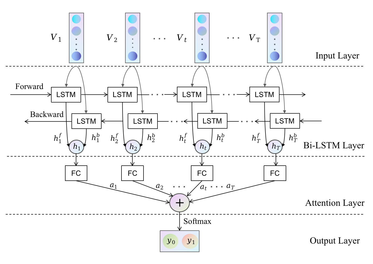
Figure 1. The network architecture of the LogRobust model

Bi-LSTM, an extension of LSTM, effectively captures bidirectional information by splitting the hidden neuron layer into forward and backward passes. The hidden states $h_{t}^{f}$ and $h_{t}^{b}$ from both directions are concatenated to form the combined hidden state $h_{t}$. To mitigate the influence of noise, an attention mechanism is introduced, assigning varying weights to log events. Implemented as a fully connected layer, the attention layer computes the attention weight $a_{t}$ for each log event. The hidden states are subsequently weighted and summed based on their respective attention weights. Finally, the resulting vector undergoes classification through a softmax layer.

LogRobust leverages an attention-based Bi-LSTM model to effectively capture contextual information in log sequences and autonomously discern the significance of distinct log events through log semantic understanding (Zhang et al., 2019). This approach has demonstrated favorable outcomes for volatile logs. In our study, we employ the attention-based Bi-LSTM neural network from LogRobust as the core of the DRL agent.

2.3. Bief Of DRL

2.3.1. Markov Decision Process

Formally, RL can be described as a Markov decision process (MDP) (Arulkumaran et al., 2017), which consists

• State: A set of all possible states $\mathcal{S}$.

• Action: A set of all possible actions $\mathcal{A}$.

• State transition function $g\left(s_{t+1}|s_{t},a_{t}\right)$: Given the current state $s_{t}$ and action $a_{t}$, it determines the probability $g(s_{t},a_{t})$ of transitioning to the next state $s_{t+1}$.

• Reward function $r(s_{t},a_{t})$: An immediate reward provided by the environment alongside the state transition.

• Discount factor $\gamma$: It represents the value of future rewards relative to current rewards, typically with $\gamma\in[0,1]$.

The MDP is utilized to determine the policy that maximizes the return. The policy $\pi(a|s)$ is a probability distribution that maps the current state to possible actions. The return $U_{t}$ is defined as the sum of immediate reward and discounted future rewards for the policy $\pi$ at time step $t$, i.e., $U_{t}=\sum_{t=0}^{T-1}{\gamma^{t}r_{t+1}}$. The objective of RL is to learn an optimal policy $\pi^{*}$ that maximizes the cumulative reward, where $\pi^{*}=argmax_{\pi}\mathbb{E}[U|\pi]$.

2.3.2. Optimal Action-value Function

The action-value function, denoted as $Q\left(s,a\right)$, represents the expected cumulative reward for an agent taking action $a$ in state $s$. It quantifies the value of choosing an action $a_{t}\in\mathcal{A}$ in a specific state $s_{t}\in\mathcal{S}$, considering long-term rewards and future states. It guides the agent in decision-making, maximizing long-term rewards.The definition is as follows:

(1) $$Q^{\pi}\left(s,a\right)=\mathbb{E}\left[U_{t}|s_{t}=s,a_{t}=a\right]$$

The optimal policy $\pi^{*}$ has an expected return that is greater than or equal to all other policies. It can be achieved by greedily selecting actions that maximize the given action-value function $Q^{\pi}\left(s,a\right)$ for each state, i.e., $\pi(s)=\arg\max_{a}{Q^{\pi}(s,a)}$. When this update equation converges, the action-value function becomes consistent across all states, resulting in the optimal policy $\pi^{*}=\arg\max Q^{*}(s,a)$ and the corresponding optimal action-value function:

(2) $$Q^{\ast}\left(s,a\right)=\max_{\pi}{\mathbb{E}\left[U_{t}|s_{t}=s,a_{t}=a,\pi\right]}$$

2.3.3. Function Approximation and the DQN

Deep Q-Network (DQN) (Mnih et al., 2015) algorithm in DRL learns the optimal action-value function (Q-value function). DQN is a Q-learning algorithm that utilizes deep neural networks $Q\left(s,a;\theta\right)$ to approximate $Q^{*}\left(s,a\right)$, incorporating a target network and experience replay (Lin, 1992) for training. The network’s parameters are denoted as $\theta$, with state s as input and Q-value as output for a given state-action pair.

The optimal action-value function can be defined using the Markov property as the Bellman equation (Bellman, 1952), which has the following recursive form:

(3) $$Q\left(s_{t},a_{t}\right)=\mathbb{E}_{s_{t+1}}\left[r_{t}+\gamma Q\left(s_{t+1},\pi\left(s_{t+1}\right)\right)\right]$$

Based on this equation,we enhance the estimation of Q by leveraging the disparity between the current Q-value estimate and the target Q-value estimate. This is accomplished by minimizing the following loss function to learn the parameters $\theta$:

(4) $$L_{i}\left(\theta_{i}\right)=\mathbb{E}_{\left(s,a,r,s^{\prime}\right)\sim\mathcal{U}\left(\varepsilon\right)}\left[\left(r+\gamma\max_{a^{\prime}}{Q\left(s^{\prime},a^{\prime};\theta^{-}_{i}\right)}-Q\left(s,a;\theta_{i}\right)\right)^{2}\right]$$

Here, $\varepsilon$ represents a small batch of transitions extracted from the stored experience $\mathcal{U}=\left\{e_{1},e_{2},\cdots,e_{t}\right\}$ for the agent’s learning. Each transition is represented by a tuple, $e_{t}=\left(s_{t},a_{t},r_{t},s_{t+1}\right)$, consisting of the current state $s_{t}$, the action $a_{t}$ taken, the reward value $r_{t}$ obtained, and the next state $s_{t+1}$ transitioned into at time step $t$. At each time step $t$, the transition $e_{t}$ obtained from the agent’s interaction with the environment is stored in the stored experience $\mathcal{U}$. $\theta_{i}$ represents the parameters of the current Q network at iteration $i$ , and $\theta_{i}^{-}$ represents the parameters of the target Q network at iteration $i$. The parameters $\theta_{i}$ of the Q network are updated in real-time, and every K steps, $\theta_{i}^{-}$ is updated with $\theta_{i}$.

2.3.4. DRL-driven Anomaly Detection

Deep reinforcement learning (DRL) has successfully achieved human-level performance in numerous tasks and has found applications in diverse and intricate domains such as natural language processing, computer vision, and more. Anomaly detection is an equally significant application of DRL.

The IVADC-FDRL model, proposed in (Mansour et al., 2021), utilizes the DQN algorithm to detect and categorize abnormal activities in videos. The DPLAN model, introduced in (Pang et al., 2021), employs DQN for intrusion detection in a weakly supervised environment with only positive instances, effectively identifying various types of attacks. (Huang et al., 2018) constructs a supervised time series anomaly detector using DQN. (Elaziz et al., 2023) utilizes DDQN (Wang et al., 2016), another widely used algorithm in DRL, to detect anomalies in business processes within a weakly supervised environment consisting of solely positive instances.

In this paper, we explore the application of deep reinforcement learning to log anomaly detection. However, unlike previous studies (Pang et al., 2021; Elaziz et al., 2023), we go beyond leveraging solely labeled anomaly data and also incorporate labeled normal data to fully exploit the available information.

3. PROPOSED APPROACH

To address the challenge of log anomaly detection in imbalanced data scenarios, where there is a small labeled set and a large unlabeled set, we propose a deep reinforcement learning framework to train an anomaly detection function $\varphi:\mathcal{D}\rightarrow\mathbb{R}$. This function is designed to assign higher anomaly scores to log sequences $s_{i}$ that are known or unknown anomaly instances compared to normal instances $s_{j}$, given that $s_{i},s_{j}\in\mathcal{D}$. Here, $\mathcal{D}$ represents the training set, which consists of a small labeled dataset $\mathcal{D}_{l}$ and a large unlabeled dataset $\mathcal{D}_{u}$, denoted as $\mathcal{D}=\{\mathcal{D}_{l},\mathcal{D}_{u}\}$.Both $\mathcal{D}_{l}$ and $\mathcal{D}_{u}$ encompass both normal and abnormal log sequences, with a significantly smaller proportion of anomaly log sequences compared to normal log sequences.

3.1. Overall Framework

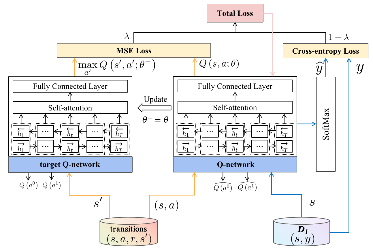
Figure 2. The overall architecture of the model

In DQNLog, we adopt a deep reinforcement learning approach to construct a log anomaly detection model. The model’s objective is to detect anomalies by approximating the optimal action value function (Q-value function). On one hand, we incorporates the DQN (Mnih et al., 2015) algorithm, which utilizes a Q-network and a target Q-network with delayed updates. The loss function is defined by the disparity between the current Q-value and the target Q-value predicted by both networks. On the other hand, we introduce an additional cross-entropy loss term to integrate the constraints of real label information into the agent’s optimization process. This prevents over-reliance on Q-value function estimation.

The overall framework of the model is shown in Figure 2, follows a loss function comprising two components. The first component is the mean squared error loss, comparing the output values of the Q-network and the target Q-network within the agent. The second component is the cross-entropy loss, evaluating dissimilarity between predicted classifications from the Q-network and the actual labels. The total loss function is the sum of these two losses. Both the Q-network and the target Q-network take sequences of log semantic vectors as input and output corresponding Q-values for classifying the log sequences as either anomaly or normal. During RL-based policy improvement, the agent utilizes the transition $(s_{t},a_{t},r_{t},s_{t+1})$ from stored experience. The Q-value for the current log sequence $s_{t}$, predicted by the Q-network for action $a_{t}$, is considered as the current Q-value. The target Q-value is the maximum Q-value of the next log sequence $s_{t+1}$, as predicted by the target Q-network. The aim is to minimize the mean squared error loss between the current Q-value and the target Q-value. Furthermore, the agent also receives a supervised signal from labeled instances in $\mathcal{D}_{l}$. The Q-network predicts Q-values for all possible actions of the labeled log sequences in $\mathcal{D}_{l}$. These predicted Q-values are then passed through a softmax function to obtain the predicted classification, aiming to minimize cross-entropy loss with the actual labels.

The agent’s parameters are updated in each iteration using two loss functions. Convergence is reached when the Q-network parameters match those of the target Q-network. The final model is then employed for log anomaly detection, taking in log semantic vector sequences. The output with the highest Q-value is deemed the final classification result.

3.2. DRL Tailored for Log Anomaly Detection

3.2.1. Foundation of the Proposed Approach

We formulate the problem of log anomaly detection in an imbalanced dataset, with few labeled instances and a large number of unlabeled instances, as a Markov Decision Process (MDP). By defining critical components such as states, agent, actions, environment, and rewards, we transform it into a Deep Reinforcement Learning (DRL) problem.

• State: The state space $\mathcal{S}=\mathcal{D}$, where each state $s\in\mathcal{S}$ represents a log semantic sequence.

• Action: The action space $\mathcal{A}=\left\{a^{0},a^{1}\right\}$, where $a^{0}$ and $a^{1}$ correspond to the actions ‘normal’ and ‘anomaly’, respectively.

• Agent: Implemented as a deep neural network, the agent aims to determine the optimal action from the action space $\mathcal{A}$.

• Environment: Simulates the agent’s interaction, accomplished through a state transition function $g\left(s_{t+1}|s_{t},a_{t}\right)$ that is biased towards anomalies.

• Rewards: The reward function is defined as $r\left(s_{t},a_{t}\right)=h\left(r^{e}|s_{t},a_{t}\right)+f\left(r^{i}|s_{t}\right)$, where $h\left(r^{e}|s_{t},a_{t}\right)$ represents the extrinsic reward given by the environment based on predicted and actual labels, and $f\left(r^{i}|s_{t}\right)$ denotes the intrinsic reward provided by the exploration mechanism to measure novelty.

3.2.2. Procedure of Our DRL-based Log Anomaly Detection

Our proposed log anomaly detection method based on DRL utilizes DQN to learn the optimal Q-value function and obtain the policy with maximum expected return. During training, the agent autonomously interacts with the environment, obtaining rewards and improving its policy to maximize cumulative rewards. The DRL-based log anomaly detection framework, depicted in Figure 3, involves the following steps:

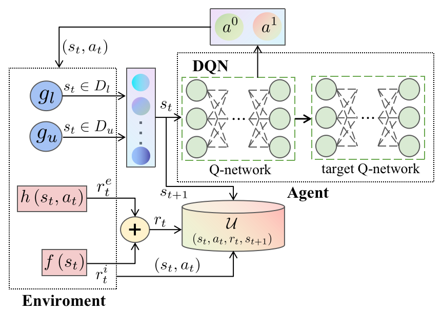
Figure 3. DRL-based log anomaly detection framework

(1)At each time step $t$, the agent interacts with the environment, obtaining state $s_{t}$ from $\mathcal{D}$ using the state transition function $g$. The agent takes action $a_{t}$ based on the maximum Q-value. Simultaneously, the agent receives reward value $r_{t}$, generated by both the external reward function $h(s_{t},a_{t})$ and the intrinsic reward function $f(s_{t})$.

(2)The state transition function $g(s_{t+1}|s_{t},a_{t})$ utilizes the current state $s_{t}$ and action $a_{t}$ to determine the succeeding state $s_{t+1}$. Additionally, the tuple $\left(s_{t},a_{t},r_{t},s_{t+1}\right)$ is stored in the stored experience $\mathcal{U}$. $g$ is designed to prioritize returning samples that are more likely to be anomalies from $\mathcal{D}_{u}$, while maintaining an equal probability of returning samples from $\mathcal{D}_{l}$.

(3)A batch size transition is randomly selected from the stored experience $\mathcal{U}$, and the delayed-updated target Q network is utilized to update the weights of the Q network through gradient descent optimization of the loss function.

(4) Iteratively repeat steps (1)-(3) to train the agent and maximize the cumulative joint reward.

Refer to Chapter 4 for the primary design strategies in DRL.

3.2.3. MSE loss of DRL method

Our DQN agent learns the optimal action-value function through time-discretization, avoiding repetitive experiments. Instead, it updates the current Q-value by incorporating the next state’s Q-value. Additionally, a delayed-updated target function is introduced in this method to alleviate instability caused by simultaneous Q value acquisition and function updates (Mnih et al., 2015).

For computational efficiency, we optimize the loss function using stochastic gradient descent rather than calculating all the expectations in formula (5). Specifically, we replace the expectation with a single sample.

(5) $$L_{i}^{1}\left(\theta_{i}\right)=\left(r+\gamma\max_{a^{\prime}}{Q\left(s^{\prime},a^{\prime};\theta_{i}^{-}\right)}-Q\left(s,a;\theta_{i}\right)\right)^{2}$$

Wherein, every K steps, set $\theta_{i}^{-}=\theta_{i-1}$.

3.3. Cross-entropy loss that stabilizes the model

The MSE loss function in Eq.(5) of the DQN evaluates the model’s performance by quantifying the disparity between predicted and target values. This guides parameter updates in the correct direction. The Q network’s output is the predicted value, while the target Q network’s output is the target value. However, it’s important to note that both predicted and target Q-values are neural network estimates, derived from propagating the Q network. Therefore, their accuracy may be compromised, leading to erroneous actions by the agent.

To prevent the agent from making erroneous actions due to inaccurate predictions and targets, we propose incorporating ground truth labels during parameter updates. This ensures reliable guidance for the agent, rather than relying solely on estimates. Zhang et al. (Zhang et al., 2018) introduced the DML strategy, which utilizes dual loss functions to facilitate mutual learning among the student network ensemble. This is achieved through the KL mimicry loss function as well as the supervised cross-entropy loss function. To ensure the agent receives supervised signals from actual label information while guided by RL, we consider sampling a subset of labeled samples and incorporating the commonly used cross-entropy loss function in classification problems during agent optimization.

(6) $$L_{i}^{2}\left(\theta_{i}\right)=-\frac{1}{M}\sum_{k=1,s_{k}\in\mathcal{D}_{l}}^{M}\left(y_{k}\cdot log\left(\widehat{y_{k}}\right)+\left(1-y_{k}\right)\cdot log\left(1-\widehat{y_{k}}\right)\right)$$

Here, $M$ represents the sample size used for cross-entropy validation, consisting of an equal number of normal and anomalous labeled samples. $y_{k}$ represents the true labels of samples $s_{k}$, while $\widehat{y_{k}}$ represents the predicted probabilities for samples $s_{k}\in\mathcal{D}_{l}$ after applying $Q\left(s_{k},a;\theta_{i}\right)$ to the softmax function. The cross-entropy loss quantifies the discrepancy between the agent’s predicted class and the true label, enabling differentiation between normal and anomalous cases even when the DRL model makes incorrect estimations. By partially suppressing substantial parameter fluctuations, our RL model is able to learn without deviating from the normal trajectory.

3.4. Dual loss function of the final model

In summary, the loss function in the DQNLog training process consists of two parts: one is the RL mean squared error loss, which makes the Q-value estimated by the Q network closer to the true Q-value; the other is the supervised cross-entropy loss, which makes the classification results predicted by the Q network consistent with the true labels. This is shown in Eq.9.

(7) $$L_{i}\left(\theta_{i}\right)=L_{i}^{1}\left(\theta_{i}\right)+\lambda L_{i}^{2}\left(\theta_{i}\right)$$

Here, $\lambda$ is a hyperparameter that balances the relative contributions of the RL mean squared error loss and the cross-entropy loss. The loss function defined in this way enables our agent to continuously improve its policy under the RL mechanism (MSE loss $L^{1}$) while also correctly predicting the training samples (cross-entropy loss $L^{2}$). This ensures that our model does not deviate from the normal trajectory even when facing “wrong estimation” in DRL.

3.5. The Algorithm of DQNLog

The training process of DQNLog is depicted in Algorithm 1. The initial three steps involve setting the weight parameters for both the Q network and the target Q network to the pre-trained LogRobust network parameters, as well as initializing the size of the stored experience. We then train DQNLog for $n\_episode$ episodes. In each episode, a state $s_{1}$ is randomly selected from $\mathcal{D}_{u}$, and training is performed for $n\_steps$ steps. In Steps 7-9, the agent employs the $\varepsilon-greedy$ exploration strategy. It randomly selects an action from $\left\{a^{0},a^{1}\right\}$ with probability $\varepsilon$; otherwise, it selects the action $t$ with the maximum Q-value. As the Q-value function improves its accuracy, $\varepsilon$ linearly decreases as the total time steps increase. In Steps 10-11, after the agent selects an action, the environment randomly returns state $s_{t+1}$ from $\mathcal{D}_{l}$ with probability $p$, otherwise it selects the state $s_{t+1}$ from a random subset $S\subset\mathcal{D}_{u}$ based on $g_{u}$, which corresponds to the state $s_{t}$ that is farthest/closest. In Steps 12-14, the environment provides a combined reward, $r_{t}$, which is the sum of an external reward, $r_{t}^{e}$, based on $h\left(s_{t},a_{t}\right)$, and an internal reward, $r_{t}^{i}$, based on $f\left(s_{t}\right)$. Afterwards, the obtained transition $\left(s_{t},a_{t},r_{t},s_{t+1}\right)$ is stored in $\mathcal{U}$. During Steps 16-22, the Q-value function is updated. Additionally, every K steps, the Q-network resets the target Q-network.

Algorithm 1 Training DQNLog

0:  $\mathcal{D}=\left\{\mathcal{D}_{l},\mathcal{D}_{u}\right\}$

0:  $Q\left(s,a;\theta^{\ast}\right)$

1:  Initialize Q with trained LogRobust network weights $\theta$

2:  Initialize target Q network with weights $\theta^{\prime}=\theta$ 

3:  Initialize the size of the stored experience $\mathcal{U}$ to $\mathcal{U}_{size}$

4:  for j = 1 to $n\_episodes$ do

5:     Initial first state $s_{1}$ randomly from $D_{u}$;

6:     for t = 1 to $n\_steps$ do

7:        With probability $\varepsilon$ select a random action $a_{t}$ from $\mathcal{A}$

8:        Otherwise select $a_{t}=\arg\max_{a}{Q\left(s_{t},a;\theta\right)}$

9:        $\varepsilon$ decays by $anneal\_rate$ per step;

10:        With probability $p$ the environment returns $s_{t+1}$ randomly from $\mathcal{D}_{l}$

11:        Otherwise returns $s_{t+1}$ from $S\subset\mathcal{D}_{u}$ based on $g_{u}$

12:        Calculate extrinsic reward $r_{t}^{e}$ based on $h\left(s_{t},a_{t}\right)$

13:        Calculate intrinsic reward $r_{t}^{i}$ based on $f\left(s_{t}\right)$

14:        Calculate reward $r_{t}=r_{t}^{e}+r_{t}^{i}$;

15:        Store transition $\left(s_{t},a_{t},r_{t},s_{t+1}\right)$ in $\mathcal{U}$

16:        Sample random minibatch of transitions $\left(s_{j},a_{j},r_{j},s_{j+1}\right)$ from $\mathcal{U}$ denoted as $\varepsilon$

17:        Set $y_{j}$=$\begin{cases}r_{j},\quad\text{if episode terminates at this step}\\ r_{j}+\gamma\max_{a}^{\prime}{Q\left(s_{j+1},a^{\prime};\theta^{\prime}\right)},\quad\text{otherwise}\\ \end{cases}$

18:        Calculate ${loss}_{1}=\left(y_{j}-Q\left(s_{j},a_{j};\theta\right)\right)^{2}$

19:        Randomly sample $\frac{M}{2}$ normal and anomaly samples $\left(s_{k},y_{k}\right)$ separately from $\mathcal{D}_{l}$

20:        Calculate ${loss}_{2}=-y_{k}\cdot log(\widehat{y_{k}})+\left(1-y_{k}\right)\cdot log(1-\widehat{y_{k}})$

21:        Calculate ${loss=loss}_{1}+{loss}_{2}$

22:        Perform a gradient descent step on loss with respect to the Q network weights $\theta$

23:        update $\theta^{\prime}=\theta$ every K steps

24:     end for

25:  end for

26:  return  Q

4. STRATEGIES OF DRL IN DQNLog

4.1. DQN-based Anomaly Detection Agent

The agent is the core in the DQNLog method, aiming to learn the optimal action-value function that evaluates actions under the optimal policy within a given state. We utilize DQN due to its effectiveness in handling high-dimensional state and action spaces, as well as its autonomous learning capability.

Furthermore, considering the temporal dynamics and instability of log data, we employ the attention-based Bi-LSTM neural network from LogRobust (Zhang et al., 2019) as the core of our DRL model agent to approximate the Q-value function. The Q-network and target Q-network of the DQN agent consist of four layers, namely the input layer, Bi-LSTM network layer, self-attention layer, and softmax layer. These layers are designed to receive log semantic vectors as input and generate two estimated Q values for normal and abnormal actions, respectively.

The agent iteratively minimizes the loss function defined in formula 9 during the learning process to update the Q-network parameters. This continues until the updated parameters match those of the target Q-network, resulting in a trained agent.

4.2. State Transition Function

The state transition function $g\left(s_{t+1}|s_{t},a_{t}\right)$ is the core of the environment, comprised of the $g_{l}$ function for exploiting $\mathcal{D}_{l}$ and the $g_{u}$ function for exploring $\mathcal{D}_{u}$. Specifically, $g_{l}$ is a random sampling function on dataset $\mathcal{D}_{l}$, while $g_{u}$ is a distance-based biased sampling function on dataset $\mathcal{D}_{u}$, specifically targeting abnormalities.

In $g_{l}$, the environment randomly selects the next state $s_{t+1}$ from dataset $\mathcal{D}_{l}$ for the current state $s_{t}$, regardless of the agent’s action, enabling the agent to equally exploit the labeled samples in $\mathcal{D}_{l}$.

In $g_{u}$, the environment biases the sampling of the next state $s_{t+1}$ towards abnormal samples from $\mathcal{D}_{u}$ by considering both the agent’s action $a_{t}$ and the Euclidean distance to $s_{t}$. This acceleration expedites the agent’s search for anomalies in large-scale imbalanced datasets, enhancing its efficiency in exploring $\mathcal{D}_{u}$. The definition of $g_{u}$ is shown in Eq.8.

(8) $$g_{u}\left(s_{t+1}|s_{t},a_{t}\right)=\begin{cases}\arg\min_{s\in S}{d\left(s_{t},s\right)},\quad\text{if }a_{t}=a^{1}\\ \arg\max_{s\in S}{d\left(s_{t},s\right)},\quad\text{if }a_{t}=a^{0}\end{cases}$$

Where $S$ is a random subset of $\mathcal{D}_{u}$, and d returns the Euclidean distance between $s_{t}$ and $s$. If $s_{t}$ is deemed abnormal (action $a^{1}$), it selects the most similar $s$ from subset $S$ as $s_{t+1}$. Conversely, if $s_{t}$ is regarded as normal (action $a^{0}$), it chooses the s from subset $S$ with the greatest difference from $s_{t}$ as $s_{t+1}$.

In DQNLog, $g_{l}$ and $g_{u}$ are used together with a $50\%$ probability, allowing our model to balance exploitation and exploration.

4.3. Reward Function

The reward value evaluates agent behavior and guides policy updates. In DQNLog, we introduce a combined reward mechanism that utilizes both the external reward function $h(s_{t},a_{t})$ and the intrinsic reward function $f(s_{t})$.

4.3.1. External reward function

The external reward assesses the agent’s anomaly detection performance, providing reward signal $r^{e}$ for action $a_{t}$ in state $s_{t}$. This encourages effective utilization of labeled data $\mathcal{D}_{l}$. The value of $r^{e}$ is determined by comparing predicted and actual labels per Eq.11.

(9) $$r_{t}^{e}=\ h\left(s_{t},a_{t}\right)=\begin{cases}r_{1},\quad\text{ for True Positive}\left(TP\right),s_{t}\in\mathcal{D}_{l}\\ r_{2},\quad\text{ for True Negative}\left(TN\right),s_{t}\in\mathcal{D}_{l}\\ -r_{3},\quad\text{ for False Positive}\left(FP\right),s_{t}\in\mathcal{D}_{l}\\ -r_{4},\quad\text{ for False Negative}\left(FP\right),s_{t}\in\mathcal{D}_{l}\\ 0,\quad\text{if }a_{t}=a^{0},s_{t}\in\mathcal{D}_{u}\\ -1,\quad\text{if }a_{t}=a^{1},s_{t}\in\mathcal{D}_{u}\end{cases}$$

Here, $r_{1},r_{2},r_{3},r_{4}>0$. TP denotes correct anomaly recognition by the agent, TN represents correct normal recognition, FP signifies false anomaly recognition, and FN indicates false normal recognition of an anomaly by the agent.

In log anomaly detection, correctly identifying anomalies holds greater significance than correctly identifying normal samples. To reflect this, we assign a higher reward value for TP and a lower reward value for TN, i.e., $r_{1}>r_{2}$. Moreover, ignoring genuine anomalies poses a higher risk than false positives, so we prioritize reporting false positives instead of overlooking anomalies. Hence, in comparison to FP, we impose a more stringent penalty for FN, i.e., $r_{4}>r_{3}$. In DQNLog, we set $r_{1}=1,r_{2}=0.1,r_{3}=0.4,r_{4}=1.5$ to incentivize the agent to fully leverage the labeled data in $\mathcal{D}_{l}$, particularly the data labeled as anomalies.

For $s_{t}$ in $\mathcal{D}_{u}$, the agent remains neutral. Despite the absence of labels in $\mathcal{D}_{u}$, its data follows real-world norms, where the majority of the data is expected to be normal. Therefore, the agent receives no reward for the vast majority of normal predictions it makes. Conversely, negative rewards are enforced to discourage over-reliance on uncertain abnormal samples.

4.3.2. Intrinsic reward function

The intrinsic reward encourages the agent to explore known and unknown anomalies in the unlabeled dataset $\mathcal{D}_{u}$. It is provided by the exploration mechanism as a reward signal $r^{i}$ when the agent takes action $a_{t}$ in state $s_{t}$. The value of $r^{i}$ is determined by evaluating a pre-trained LogRobust model based on Eq.12.

(10) $$r_{t}^{i}=f\left(s_{t}\right)=\begin{cases}1-\frac{rob_{p}}{\delta},\quad rob_{p}<\delta\\ \left(\frac{rob_{p}-\delta}{1-\delta}\right),\quad rob_{p}\geqslant\delta\end{cases}$$

Where ${rob}_{p}\in\left[0,1\right]$ denotes the probability predicted by the LogRobust model for the normalcy of the current state $s_{t}$. We set the confidence threshold, $\delta$, to 0.2. If ${rob}_{p}<\delta$, $s_{t}$ is deemed abnormal, and $r_{t}^{i}$ falls within $(0,1]$. Conversely, if ${rob}_{p}\geqslant\delta$, $s_{t}$ is considered normal, and $r_{t}^{i}$ falls within $[-1,0]$. When ${rob}_{p}$ approaches 0, $s_{t}$ is highly abnormal, prompting a high reward to encourage exploration of novel states. Conversely, if ${rob}_{p}$ approaches 1, $s_{t}$ is confidently normal, and no reward is given to prevent biased exploration of normal states by the agent.

In order to achieve the agent’s exploitation of $\mathcal{D}_{l}$ and the exploration of $\mathcal{D}_{u}$, we define the final reward as Equation 11.

(11) $$r=r^{i}+r^{e}$$

5. EXPERIMENTS

In our study, we assess our method by addressing the following research questions:

• How effective is DQNLog in detecting log anomalies?

• Does the cross-entropy loss term impact DQNLog’s performance?

• How do hyperparameter values affect DQNLog?

5.1. Datasets

We evaluate DQNLog’s performance on three widely used log datasets: HDFS (Xu et al., 2009), BGL (Oliner and Stearley, 2007), and Thunderbird (Oliner and Stearley, 2007). These datasets contain real-world data, annotated either manually by system administrators or automatically with alert tags. Brief descriptions of each dataset are provided below:

(1) HDFS: The HDFS dataset is sourced from the Hadoop Distributed File System (HDFS). It is generated by running MapReduce jobs on over 200 Amazon EC2 nodes and labeled by Hadoop domain experts. In total, 11,172,157 log messages were generated from 29 events, which can be grouped into 16,838 log sequences based on $block\_id$, with approximately $2.9\%$ indicating system anomalies.

(2) BGL:The BGL dataset was generated by the Blue Gene/L (BGL) supercomputer at Lawrence Livermore National Laboratory. It was manually labeled by BGL domain experts. It consists of 4,747,963 log messages from 376 events, with 348,460 flagged as abnormal $(7.34\%)$. Log messages in the BGL dataset can be grouped by $node\_id$.

(3) Thunderbird: The Thunderbird dataset was generated by a Thunderbird microprocessor supercomputer deployed at Sandia National Laboratories (SNL) and manually labeled as normal or anomalous. It is a large dataset with over 200 million log messages. Among the more than one million consecutive log data collected for time calculation, 4,934 $(0.49\%)$ were identified as abnormal (Le and Zhang, 2022). The log messages in the Thunderbird dataset can be grouped into sliding windows.

In our experiment, we randomly sampled and used 6,000 normal log sequences and 6,000 abnormal log sequences from each dataset maintained by Loghub (He et al., 2020) for training purposes. Table 1 presents the comprehensive statistics for these three datasets, including the column ‘$\#LogKeys$’ which represents the total count of distinct log templates extracted using the Drain (He et al., 2017) technique.

Table 1. Statistics of datasets

Dataset	$\#$Log Message	$\#$Anomalies	$\#$Log Keys	$\#$Log Sequences for training
				Normal	Anomaly
HDFS	11,172,157	16,838(blocks)	47	6000	6000
BGL	4,747,963	348,460(logs)	346	6000	6000
Thunderbird	20,000,000	4934(logs)	815	6000	6000

5.2. Implementation and Environment

The experiments were conducted on a Linux server with Ubuntu 18.04, equipped with an NVIDIA Tesla P40 GPU, 56GB of memory, and a 6-core CPU. DQNLog, implemented in Python and PyTorch, utilizes the open-source Keras-rl library for reinforcement learning. The Q network is configured with a hidden layer size of 128. The mini-batch size (M) is set to 32, with a learning rate of 0.001. Experience storage has a capacity of 100,000, while the sub-sample set $(S)$ has a size of 1,000. The initial exploration rate $(\varepsilon)$ is set to 1 and decreases to 0.1. After 5 pre-warming episodes, DQNLog updates the Q network parameters every episode, which consists of 2000 steps. The target Q network is updated every 5 episodes, while other hyperparameters remain the same as the default settings in [20], including a discount factor of $\gamma=0.99$ and a gradient momentum of momentum=0.95.

5.3. Evaluation Metrics

To assess the performance of DQNLog, we categorize the classification outcomes as TP, TN, FP, and FN, and employ precision, recall, and F1-score as evaluation metrics. The definitions and formulas for these three metrics are as follows:

Precision: The ratio of true positive results to the total number of log sequences predicted as anomalous. A higher precision indicates a greater proportion of actual anomalous log sequences among the predicted ones. The precision formula is: $Precision=\frac{TP}{\left(TP+FP\right)}$.

Recall: The ratio of true anomalous log sequences correctly identified as anomalous. A higher recall indicates a greater proportion of detected anomalous log sequences. The recall formula is: $Recall=\frac{TP}{\left(TP+FN\right)}$.

F1-Score: The harmonic mean of precision and recall, where higher values indicate better model performance. The F1-Score formula is: $F1-Score=\frac{\left(2*Precision*Recall\right)}{\left(Precision+Recall\right)}$.

Due to data imbalance in log anomaly detection, models tend to prioritize learning from majority normal instances. Hence, we focus on precision and recall that prioritize anomalies. Furthermore, given the practical significance of log anomaly detection in current software systems, the risk of missed anomalies outweighs false alarms. Consequently, we give higher emphasis to recall and F1-Score compared to precision.

5.4. Compared Approaches

We compare our semi-supervised model, DQNLog, with existing supervised, semi-supervised, and unsupervised log-based anomaly detection algorithms.

• PCA (Xu et al., 2009): The top k principal components and the residual components of the log count vector are projected onto the normal and anomaly subspaces. Classification of a log sequence into normal or anomaly subspace depends on its projection.

• LogClustering (Lin et al., 2016): Log sequences undergo hierarchical clustering, considering the weighting of log events. The centroid of each resulting cluster becomes the representative log sequence. Comparing distances between the log sequence and centroids enables identification of normal or anomalous sequences.

• Invariant Mining (Lou et al., 2010): By extracting sparse and integer invariants from log count vectors, it reveals the inherent linear characteristics of program workflows and flags log sequences not adhering to the invariants as anomalies.

• LogRobust (Zhang et al., 2019): The log events are aggregated using TF-IDF weighting with pre-trained word vectors from FastText (Joulin et al., 2016), extracting their semantic information. This information is represented as semantic vectors, which are input into an attention-based Bi-LSTM model to detect anomalies.

• PLELog (Yang et al., 2021): The dimensionality-reduced log semantic vectors are clustered using the HDBSCAN algorithm. Similar vectors are grouped together, and unmarked log sequences are assigned probability labels based on known normal labels within each cluster. These probability labels indicate the likelihoods of log sequence categories, rather than providing definite labels. Build an attention-based GRU neural network model for anomaly detection, leveraging the labeled training set estimated via probability labels.

For the mentioned methods, we utilize Drain (He et al., 2017) for parsing logs and extracting log events, as recent benchmarks (Zhu et al., 2019; He et al., 2016b) have established Drain as an accurate log parser with superior efficiency and precision.Additionally, we employed loglizer (He et al., 2016a), an open-source log analysis toolkit developed by The Chinese University of Hong Kong, to evaluate the PCA, LogClustering, and Invariant Mining methods.

5.5. Results and Analysis

To ensure consistency with real-world anomaly scenarios, we closely matched the anomaly contamination rates in the dataset to the actual situations. Specifically, within the training set, the anomaly contamination rates were set to $3\%$, $7\%$, and $1\%$ for the HDFS, BGL, and Thunderbird datasets, respectively. We randomly sampled logs from 6,000 normal log sequences and 6,000 anomalous log sequences to create a small labeled dataset, $\mathcal{D}_{l}$, and a large unlabeled dataset, $\mathcal{D}_{u}$, following ratios of 1:9, 2:8, and 3:7 respectively. Moreover, the proportion of anomalous data in both $\mathcal{D}_{l}$ and $\mathcal{D}_{u}$ was strictly controlled. Three sets of experiments were conducted for each dataset, and Table 2 presents the statistics on the quantity of experimental data.

Table 2. Statistics on the amount of experimental data

$\bm{\mathcal{D}_{l}:\mathcal{D}_{u}}$	Dataset	$\bm{\mathcal{D}_{l}}$	$\bm{\mathcal{D}_{u}}$	all
1:9	HDFS	618	5567	6185
	BGL	645	5806	6451
	Thunderbird	606	5454	6060
2:8	HDFS	1237	4948	6185
	BGL	1290	5161	6451
	Thunderbird	1212	4848	6060
2:8	HDFS	1855	4328	6183
	BGL	1935	4516	6451
	Thunderbird	1818	4242	6060

$\bm{\left(1\right)}$ RQ1: The effectiveness of DQNLog

Tables 3 and 4 display results of various methodologies on the HDFS, BGL, and Thunderbird datasets, including precision, recall, and F1-score. Data ratios of $\mathcal{D}_{l}$ and $\mathcal{D}_{u}$ were maintained at 2:7 and 3:8, respectively. Despite a small data volume, significant asymmetry between labeled and unlabeled samples, and highly imbalanced distribution of abnormal and normal samples, DQNLog demonstrated strong performance, particularly in improving recall and F1-score.

The table highlights the subpar performance of traditional machine learning methods (e.g., PCA, LogClustering, and IM) in log anomaly detection, primarily due to their exclusive dependence on log count vectors, which overlooks correlations and semantic relationships among logs. Moreover, these methods demonstrate notable superiority on the HDFS dataset relative to BGL and Thunderbird datasets, likely because of HDFS’s simpler log event types and shorter time span, resulting in fewer instances of unstable data.

Deep learning methods like LogRobust and PLELog generally outperform traditional machine learning methods in log anomaly detection. They demonstrate superior processing capabilities on datasets like BGL and Thunderbird, which span longer time periods and contain diverse log event types. These models effectively capture temporal correlation and semantic embedding of logs, leveraging historical and semantic information to handle unstable log data. However, deep learning models face a challenge when dealing with highly imbalanced data and limited labeled samples. They either focus solely on learning existing anomalies in the training set or struggle to achieve high precision, recall, and F1-score simultaneously. For example, the LogRobust model achieved high precision but had difficulties with recall and F1-score when applied to the HDFS dataset.

The experimental results demonstrate that DQNLog effectively enhances the recall rate and F1-score, while maintaining precision. Furthermore, the practical context introduced by DQNLog enhances its applicability in real-world scenarios. In contrast to PLELog, another semi-supervised method, DQNLog achieves improvements in precision and F1-score by not only leveraging normal log sequences but also utilizing partially labeled anomalies.

Table 3. Experimental results for $\mathcal{D}_{l}:\mathcal{D}_{u}=2:8$

Dataset	Method	Precision	Recall	F1-score
HDFS	PLELog	0.242	0.872	0.379
	LogRobust	1.000	0.372	0.542
	DQNLog	0.988	0.574	0.727
BGL	PLELog	0.336	0.983	0.501
	LogRobust	0.908	0.712	0.798
	DQNLog	0.954	0.812	0.877
Thunderbird	PLELog	0.068	0.875	0.126
	LogRobust	0.903	0.583	0.709
	DQNLog	0.923	0.729	0.828

Table 4. Experimental results for $\mathcal{D}_{l}:\mathcal{D}_{u}=3:7$

Dataset	Method	Precision	Recall	F1-score
HDFS	PLELog	0.259	0.938	0.406
	LogRobust	1.000	0.364	0.534
	DQNLog	0.989	0.721	0.834
BGL	PLELog	0.433	0.993	0.603
	LogRobust	0.731	0.601	0.660
	DQNLog	0.927	0.880	0.902
Thunderbird	PLELog	0.045	0.976	0.086
	LogRobust	1.000	0.190	0.320
	DQNLog	0.972	0.762	0.897

5.6. Ablation Study

To validate the added cross-entropy loss term, we compared DQNLog with its variant $DQNLog_{no\_cross}$ using the same experimental setup and dataset. Figure 4 shows the training progress of both models on the HDFS dataset with a 3:7 ratio of labeled to unlabeled data. The graph displays changes in precision, recall, and F1 score as training steps increase.

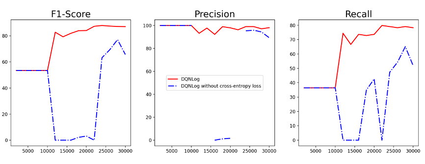
Figure 4. Experimental results of DQNLog and its variants

$\bm{\left(2\right)}$ RQ2: The impact of the added cross-entropy loss term on DQNLog

From the figure 4, it can be observed that after the preheating phase, $DQNLog_{no\_cross}$ may have inferior performance compared to the model initialized with pre-trained LogRobust when the model parameters are initially updated. This difference in performance could be attributed to the randomness in sampling from the stored experience and the inaccuracy of initial transitions. Despite gradual improvement and enhanced performance over time, $DQNLog_{no\_cross}$ does not possess the same level of advantage as DQNLog. For instance, in the HDFS dataset with a data ratio of 3:7, DQNLog exhibited an $18.58\%$ increase in F1-score and a $25.8\%$ boost in recall rate compared to $DQNLog_{no\_cross}$.

In conclusion, integrating the cross-entropy loss term significantly improves the overall performance of DQNLog. It effectively prevents the model from blindly exploring anomalies solely based on reward mechanisms, and instead guides it with reliable label information.

5.7. Hyperparameter analysis

To evaluate the impact of the hyperparameter $\lambda$ on model performance in the DQNLog loss function, we conducted experiments comparing $\lambda$ values of 0, 0.5, 1, and 2. The experiments were carried out under identical conditions using the same dataset. Figure 5 illustrates the changes in precision, recall, and F1 score during the training of the model with different $\lambda$ values on the BGL dataset, with a 2:8 ratio of labeled to unlabeled data.

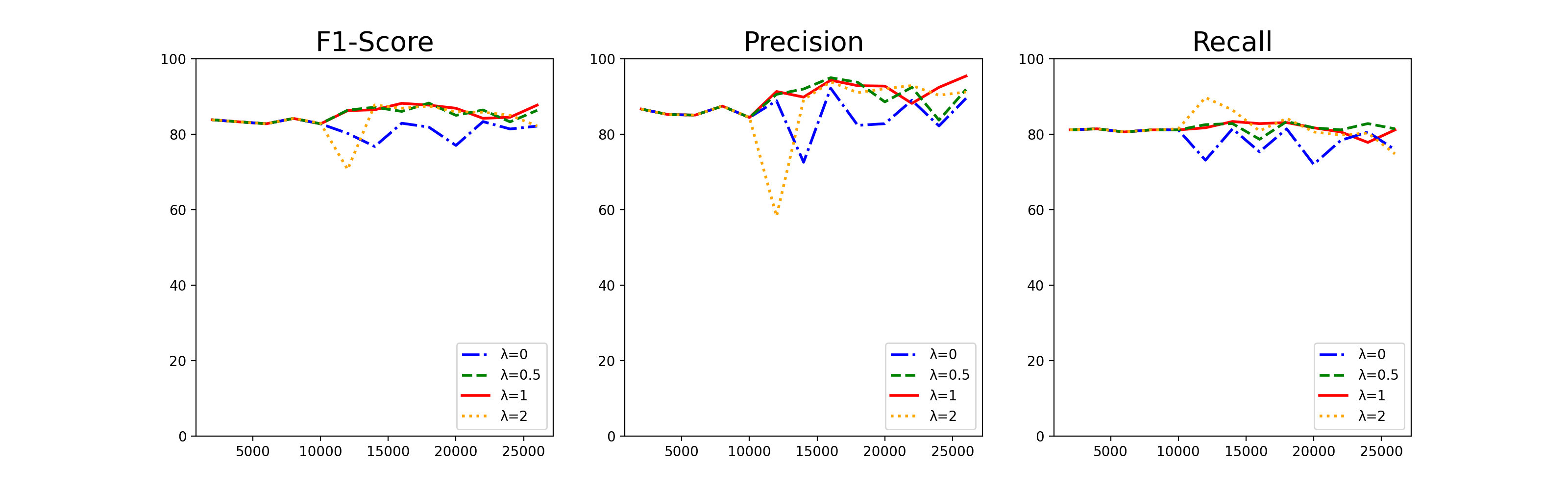
Figure 5. Experimental results for different values of $\lambda$

$\bm{\left(3\right)}$ RQ3: The impact of hyperparameter values in DQNLog

Based on the figure 5, the model shows significant fluctuations in precision, recall, and F1 scores during training at $\lambda=2$. In contrast, at $\lambda=0.5$ or $\lambda=1$, the model’s performance metrics exhibit more stable changes. This suggests that the instability in model performance might be caused by excessive amplification of the cross-entropy loss term. Increasing $\lambda$ from 0.5 to 1 slightly improves the overall model performance by enhancing the effective utilization of information derived from real labels.

Therefore, it is crucial to choose appropriate hyperparameter values. Oversized hyperparameters can result in model instability, while undersized hyperparameters may overlook genuine label information in the log sequence, ultimately reducing the amount of captured information.

6. CONCLUSION

Log anomaly detection is essential for ensuring the security and maintenance of modern software systems. This paper introduces DQNLog, a semi-supervised method for detecting anomalies in log data. Unlike existing log anomaly detection methods, we integrate it with deep reinforcement learning. In this approach, the agent is motivated by external rewards to learn from both known anomalous and normal information, enhancing the model’s detection accuracy. Additionally, driven by internal rewards, the agent actively explores unknown anomalies, enabling the model to learn more generalized anomalies. Furthermore, by introducing a state transition function that favors anomalies, DQNLog is more inclined to sample abnormal instances, thereby partially addressing the issue of data imbalance. Furthermore, an additional cross-entropy loss term has been incorporated into the loss function of DQNLog. This allows the model to leverage the true label information directly during parameter updating, thereby mitigating the deviation caused by model ”mis-estimation” to some extent. Experimental results on three widely used log datasets show that DQNLog outperforms existing log anomaly detection methods in scenarios with limited labeled samples, abundant unlabeled samples, and imbalanced data distributions.

- (1)
- Arulkumaran et al. (2017) Kai Arulkumaran, Marc Peter Deisenroth, Miles Brundage, and Anil Anthony Bharath. 2017. Deep reinforcement learning: A brief survey. IEEE Signal Processing Magazine 34, 6 (2017), 26–38.
- Bellman (1952) Richard Bellman. 1952. On the theory of dynamic programming. Proceedings of the national Academy of Sciences 38, 8 (1952), 716–719.
- Bodik et al. (2010) Peter Bodik, Moises Goldszmidt, Armando Fox, Dawn B Woodard, and Hans Andersen. 2010. Fingerprinting the datacenter: automated classification of performance crises. In Proceedings of the 5th European conference on Computer systems. 111–124.
- Breunig et al. (2000) Markus M Breunig, Hans-Peter Kriegel, Raymond T Ng, and Jörg Sander. 2000. LOF: identifying density-based local outliers. In Proceedings of the 2000 ACM SIGMOD international conference on Management of data. 93–104.
- Chen et al. (2004) Mike Chen, Alice X Zheng, Jim Lloyd, Michael I Jordan, and Eric Brewer. 2004. Failure diagnosis using decision trees. In International Conference on Autonomic Computing, 2004. Proceedings. IEEE, 36–43.
- Du and Li (2016) Min Du and Feifei Li. 2016. Spell: Streaming parsing of system event logs. In 2016 IEEE 16th International Conference on Data Mining (ICDM). IEEE, 859–864.
- Du et al. (2017) Min Du, Feifei Li, Guineng Zheng, and Vivek Srikumar. 2017. Deeplog: Anomaly detection and diagnosis from system logs through deep learning. In Proceedings of the 2017 ACM SIGSAC conference on computer and communications security. 1285–1298.
- Elaziz et al. (2023) Eman Abd Elaziz, Radwa Fathalla, and Mohamed Shaheen. 2023. Deep reinforcement learning for data-efficient weakly supervised business process anomaly detection. Journal of Big Data 10, 1 (2023), 33.
- Fu et al. (2009) Qiang Fu, Jian-Guang Lou, Yi Wang, and Jiang Li. 2009. Execution anomaly detection in distributed systems through unstructured log analysis. In 2009 ninth IEEE international conference on data mining. IEEE, 149–158.
- He et al. (2016b) Pinjia He, Jieming Zhu, Shilin He, Jian Li, and Michael R Lyu. 2016b. An evaluation study on log parsing and its use in log mining. In 2016 46th annual IEEE/IFIP international conference on dependable systems and networks (DSN). IEEE, 654–661.
- He et al. (2017) Pinjia He, Jieming Zhu, Zibin Zheng, and Michael R Lyu. 2017. Drain: An online log parsing approach with fixed depth tree. In 2017 IEEE international conference on web services (ICWS). IEEE, 33–40.
- He et al. (2021) Shilin He, Pinjia He, Zhuangbin Chen, Tianyi Yang, Yuxin Su, and Michael R Lyu. 2021. A survey on automated log analysis for reliability engineering. ACM computing surveys (CSUR) 54, 6 (2021), 1–37.
- He et al. (2016a) Shilin He, Jieming Zhu, Pinjia He, and Michael R Lyu. 2016a. Experience report: System log analysis for anomaly detection. In 2016 IEEE 27th international symposium on software reliability engineering (ISSRE). IEEE, 207–218.
- He et al. (2020) Shilin He, Jieming Zhu, Pinjia He, and Michael R Lyu. 2020. Loghub: A large collection of system log datasets towards automated log analytics. arXiv preprint arXiv:2008.06448 (2020).
- Huang et al. (2018) Chengqiang Huang, Yulei Wu, Yuan Zuo, Ke Pei, and Geyong Min. 2018. Towards experienced anomaly detector through reinforcement learning. In Proceedings of the AAAI Conference on Artificial Intelligence, Vol. 32.
- Joulin et al. (2016) Armand Joulin, Edouard Grave, Piotr Bojanowski, Matthijs Douze, Hérve Jégou, and Tomas Mikolov. 2016. Fasttext. zip: Compressing text classification models. arXiv preprint arXiv:1612.03651 (2016).
- Le and Zhang (2022) Van-Hoang Le and Hongyu Zhang. 2022. Log-based anomaly detection with deep learning: How far are we?. In Proceedings of the 44th international conference on software engineering. 1356–1367.
- Liang et al. (2007) Yinglung Liang, Yanyong Zhang, Hui Xiong, and Ramendra Sahoo. 2007. Failure prediction in ibm bluegene/l event logs. In Seventh IEEE International Conference on Data Mining (ICDM 2007). IEEE, 583–588.
- Lin (1992) Long-Ji Lin. 1992. Self-improving reactive agents based on reinforcement learning, planning and teaching. Machine learning 8 (1992), 293–321.
- Lin et al. (2016) Qingwei Lin, Hongyu Zhang, Jian-Guang Lou, Yu Zhang, and Xuewei Chen. 2016. Log clustering based problem identification for online service systems. In Proceedings of the 38th International Conference on Software Engineering Companion. 102–111.
- Liu et al. (2008) Fei Tony Liu, Kai Ming Ting, and Zhi-Hua Zhou. 2008. Isolation forest. In 2008 eighth ieee international conference on data mining. IEEE, 413–422.
- Lou et al. (2010) Jian-Guang Lou, Qiang Fu, Shenqi Yang, Ye Xu, and Jiang Li. 2010. Mining invariants from console logs for system problem detection. In 2010 USENIX Annual Technical Conference (USENIX ATC 10).
- Makanju et al. (2009) Adetokunbo AO Makanju, A Nur Zincir-Heywood, and Evangelos E Milios. 2009. Clustering event logs using iterative partitioning. In Proceedings of the 15th ACM SIGKDD international conference on Knowledge discovery and data mining. 1255–1264.
- Mansour et al. (2021) Romany F Mansour, José Escorcia-Gutierrez, Margarita Gamarra, Jair A Villanueva, and Nallig Leal. 2021. Intelligent video anomaly detection and classification using faster RCNN with deep reinforcement learning model. Image and Vision Computing 112 (2021), 104229.
- Meng et al. (2019) Weibin Meng, Ying Liu, Yichen Zhu, Shenglin Zhang, Dan Pei, Yuqing Liu, Yihao Chen, Ruizhi Zhang, Shimin Tao, Pei Sun, et al. 2019. Loganomaly: Unsupervised detection of sequential and quantitative anomalies in unstructured logs.. In IJCAI, Vol. 19. 4739–4745.
- Mnih et al. (2015) Volodymyr Mnih, Koray Kavukcuoglu, David Silver, Andrei A Rusu, Joel Veness, Marc G Bellemare, Alex Graves, Martin Riedmiller, Andreas K Fidjeland, Georg Ostrovski, et al. 2015. Human-level control through deep reinforcement learning. nature 518, 7540 (2015), 529–533.
- Oliner and Stearley (2007) Adam Oliner and Jon Stearley. 2007. What supercomputers say: A study of five system logs. In 37th annual IEEE/IFIP international conference on dependable systems and networks (DSN’07). IEEE, 575–584.
- Pang et al. (2021) Guansong Pang, Anton van den Hengel, Chunhua Shen, and Longbing Cao. 2021. Toward deep supervised anomaly detection: Reinforcement learning from partially labeled anomaly data. In Proceedings of the 27th ACM SIGKDD conference on knowledge discovery & data mining. 1298–1308.
- Vaarandi (2003) Risto Vaarandi. 2003. A data clustering algorithm for mining patterns from event logs. In Proceedings of the 3rd IEEE Workshop on IP Operations & Management (IPOM 2003)(IEEE Cat. No. 03EX764). Ieee, 119–126.
- Vaarandi and Pihelgas (2015) Risto Vaarandi and Mauno Pihelgas. 2015. Logcluster-a data clustering and pattern mining algorithm for event logs. In 2015 11th International conference on network and service management (CNSM). IEEE, 1–7.
- Wang et al. (2016) Ziyu Wang, Tom Schaul, Matteo Hessel, Hado Hasselt, Marc Lanctot, and Nando Freitas. 2016. Dueling network architectures for deep reinforcement learning. In International conference on machine learning. PMLR, 1995–2003.
- Xu et al. (2009) Wei Xu, Ling Huang, Armando Fox, David Patterson, and Michael I Jordan. 2009. Detecting large-scale system problems by mining console logs. In Proceedings of the ACM SIGOPS 22nd symposium on Operating systems principles. 117–132.
- Yang et al. (2021) Lin Yang, Junjie Chen, Zan Wang, Weijing Wang, Jiajun Jiang, Xuyuan Dong, and Wenbin Zhang. 2021. Semi-supervised log-based anomaly detection via probabilistic label estimation. In 2021 IEEE/ACM 43rd International Conference on Software Engineering (ICSE). IEEE, 1448–1460.
- Zhang et al. (2019) Xu Zhang, Yong Xu, Qingwei Lin, Bo Qiao, Hongyu Zhang, Yingnong Dang, Chunyu Xie, Xinsheng Yang, Qian Cheng, Ze Li, et al. 2019. Robust log-based anomaly detection on unstable log data. In Proceedings of the 2019 27th ACM Joint Meeting on European Software Engineering Conference and Symposium on the Foundations of Software Engineering. 807–817.
- Zhang et al. (2018) Ying Zhang, Tao Xiang, Timothy M Hospedales, and Huchuan Lu. 2018. Deep mutual learning. In Proceedings of the IEEE conference on computer vision and pattern recognition. 4320–4328.
- Zhu et al. (2019) Jieming Zhu, Shilin He, Jinyang Liu, Pinjia He, Qi Xie, Zibin Zheng, and Michael R Lyu. 2019. Tools and benchmarks for automated log parsing. In 2019 IEEE/ACM 41st International Conference on Software Engineering: Software Engineering in Practice (ICSE-SEIP). IEEE, 121–130.