Estimating the Lateral Motion States of an Underwater Robot by Propeller Wake Sensing Using an Artificial Lateral Line

Abstract

An artificial lateral line (ALL) is a bioinspired flow sensing system of an underwater robot that consists of distributed flow sensors. The ALL has achieved great success in sensing the motion states of bioinspired underwater robots, e.g., robotic fish, that are driven by body undulation and/or tail flapping. However, the ALL has not been systematically tested and studied in the sensing of underwater robots driven by rotating propellers due to the highly dynamic and complex flow field therein. This paper makes a bold hypothesis that the distributed flow measurements sampled from the propeller wake flow, although infeasible to represent the entire flow dynamics, provides sufficient information for estimating the lateral motion states of the leader underwater robot. An experimental testbed is constructed to investigate the feasibility of such a state estimator which comprises a cylindrical ALL sensory system, a rotating leader propeller, and a water tank with a planar sliding guide. Specifically, a hybrid network that consists of a one-dimensional convolution network (1DCNN) and a bidirectional long short-term memory network (BiLSTM) is designed to extract the spatiotemporal features of the time series of distributed pressure measurements. A multi-output deep learning network is adopted to estimate the lateral motion states of the leader propeller. In addition, the state estimator is optimized using the whale optimization algorithm (WOA) considering the comprehensive estimation performance. Extensive experiments are conducted the results of which validate the proposed data-driven algorithm in estimating the motion states of the leader underwater robot by propeller wake sensing.

I Introduction

In the nature, the lateral line is an essential class of fish’s flow-sensing organ that plays a crucial role in their flow-relative behaviors such as obstacle avoidance, rheotaxis, predation, and schooling[1, 2]. Consisting of superficial and canalicular neuromasts, the lateral line measures the fluid vibration and the pressure gradient to perceive the surrounding flow environment[3]. Taking the inspiration therein, researchers have designed various artificial lateral line systems (ALLs) aiming to enhance the flow-sensing capability of bioinspired underwater robots[4, 5, 6, 7, 8, 9, 10, 11].

Most existing research on the ALL has focused on the sensing of flow fields generated by either bioinspired robotic fish with body/fin undulations or dipoles with periodic oscillations. Generally speaking, such flow fields are tractable and represented by either analytical potential flow models[12, 13] or regular vortex street models[14, 15]. Based on these hidden flow models, the sensory measurements of the ALL are sufficient to capture the main coherent flow structures, thus leading to successful estimation of the flow field of interest. However, the majority of underwater robots used in the real world are equipped with high-speed rotating propellers[16, 17, 18], whose wake flows are highly dynamic and complex compared to those of bioinspired fish robots[19, 20, 21, 22, 23]. The modeling and analysis of the propeller wake typically requires high-precision and high-sensitivity computational fluid dynamics simulation, which is computationally expensive inhibiting real-time flow sensing[24, 25]. The dynamic and complex flow field of the propeller wake presents a significant challenge for the application of the ALL therein. Therefore, although many successful designs and applications of ALLs have been demonstrated, there still remains an open question whether ALLs are capable of providing sufficient feedback information for flow sensing of propeller-driven underwater robots, and if yes, how to design an estimation algorithm to assimilate the distributed measurements.

To address the aforementioned problem, this paper investigates the feasibility and the algorithmic design of sensing the wake flow of a high-speed rotating propeller using an ALL. This paper takes a bold hypothesis that the distributed pressure measurement data sampled by the ALL from the highly dynamic and complex wake flow, although cannot represent the entire flow dynamics, is still sufficiently rich for estimating the relative motion states of the leader propeller-driven underwater robot in a leader-follower formation. While the relative longitudinal or forward-backward movement is an important factor in the leader-follower formation control, the lateral or side-to-side movement is more critical for the success of following the leader using the ALL. Therefore, this paper focuses on the estimation of relative lateral motion states of a leader underwater robot.

This paper first designs an ALL with low-cost commercial pressure sensors and a corresponding testbed with data collection devices and motion control module. Extensive experiments are conducted using the designed testbed in a testing pool. To address the problem of flow sensing in the highly dynamic and stochastic propeller wake, this paper adopts a one-dimension convolution neutral network (1DCNN) and a bi-directional long short-term memory neural network (BiLSTM) to extract the spatiotemporal characteristics of the time series data of the pressure measurements collected by the ALL. To simultaneously estimate multiple lateral motion states of a propeller-driven leader robot including the displacement, the velocity magnitude, and the direction of the velocity, a multi-output deep learning network is adopted and trained based on the experimental data. The whale optimization algorithm (WOA) is used to optimize the task weights to improve the overall estimation performance.

The contributions of this paper are twofold. First, this paper presents, to the best of the authors’ knowledge, the first efforts to investigate the feasibility and the algorithmic design of flow sensing with highly dynamic and complex propeller wake using an ALL in a leader-follower formation of underwater robots. A testbed is designed and extensive experiments are conducted to provide insights into this challenging problem. Second, this paper proposes a data-driven algorithm for estimating the lateral motion states of the propeller-driven leader robot using the ALL. The algorithm integrates 1DCNN and BiLSTM to extract spatiotemporal flow features as well as a multi-output deep neutral network for the lateral motion state estimation. In addition, to improve the accuracy of the estimation results, the task weights of the loss function designed for the multi-state estimation are optimized using the bioinspired WOA algorithm.

II Problem Description

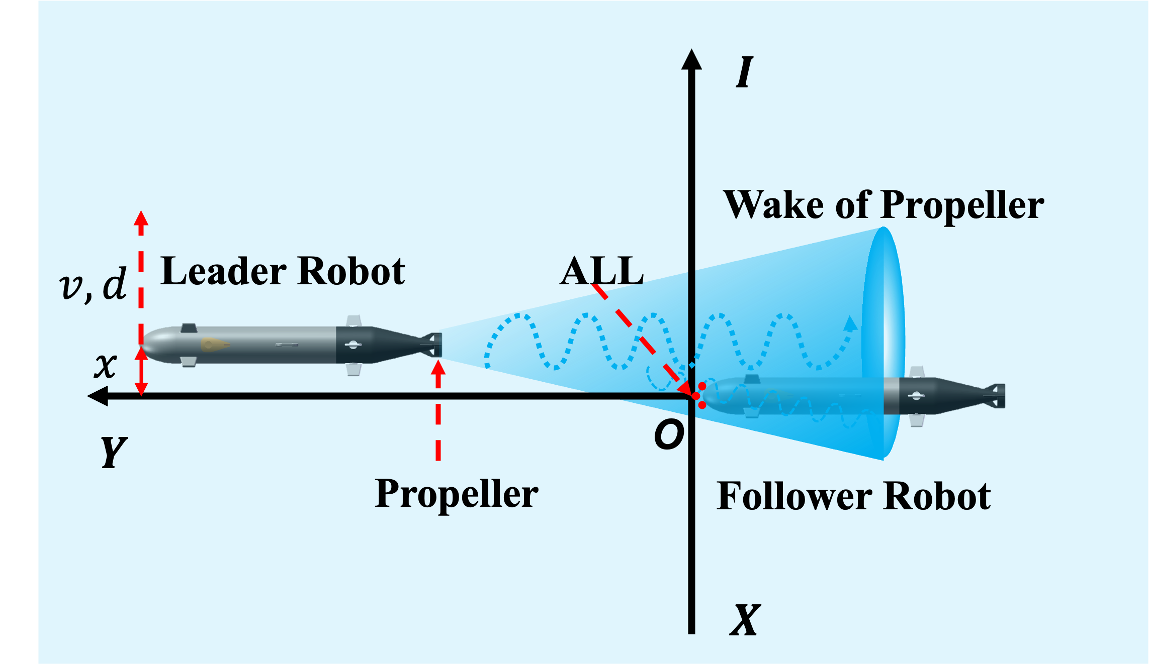
Figure 1: Illustration of the ALL sensing the propeller wake of a leader underwater robot in a leader-follower formation (Top View).

Leader-follower formation is one of the most commonly-used formation configuration in underwater robots[26]. Analogous to the lateral line of biological fish in sensing a leader fish, the ALL is expected to estimate the corresponding motion states of the leader robot by sampling its wake flow (Fig. 1). Particularly, we are more interested in sensing the lateral motion of the leader compared to the longitudinal motion which has a significant influence on the formation control. Unlike the robotic fish whose wake flow is typically generated by the body undulation and/or fin flapping, underwater robots driven by propellers have much more complex wake structures coming from the interaction of the high-speed rotating propellers and the surrounding fluid. In this paper, we hypothesize that the spatiotemporal flow measurement data acquired by the ALL, although only contains partial coherent flow information of the highly dynamic propeller wake, holds sufficient information regarding the lateral motion of the leader robot, which is described by the velocity magnitude, the velocity direction and the displacement.

II-A Testing Platform

The wake of a propeller-driven underwater robot travelling through aquatic environments is mainly dominated by the propeller wake, therefore, this paper simplifies the problem and focuses on the estimation of the motion states of a leading propeller. For this purpose, we have constructed a testing apparatus shown in Fig. 2. This experimental testbed mainly consists of a testing water tank, a high-precision sliding guide, a data acquisition system and a leader propeller. The water tank is 3m long, 2m wide and 1.5m deep. The sliding guide provides support and high-precision movement between the rotating propeller and the ALL system. A high-performance industrial personal computer (IPC) controls the sliding guide with a linear travelling velocity between 0.2 m/min and 1.2 m/min and a positional accuracy of 1 mm. Similarly to a towing tank, the sliding guide is rigidly attached to the water tank and is controllable through preprogramming or manual operation.

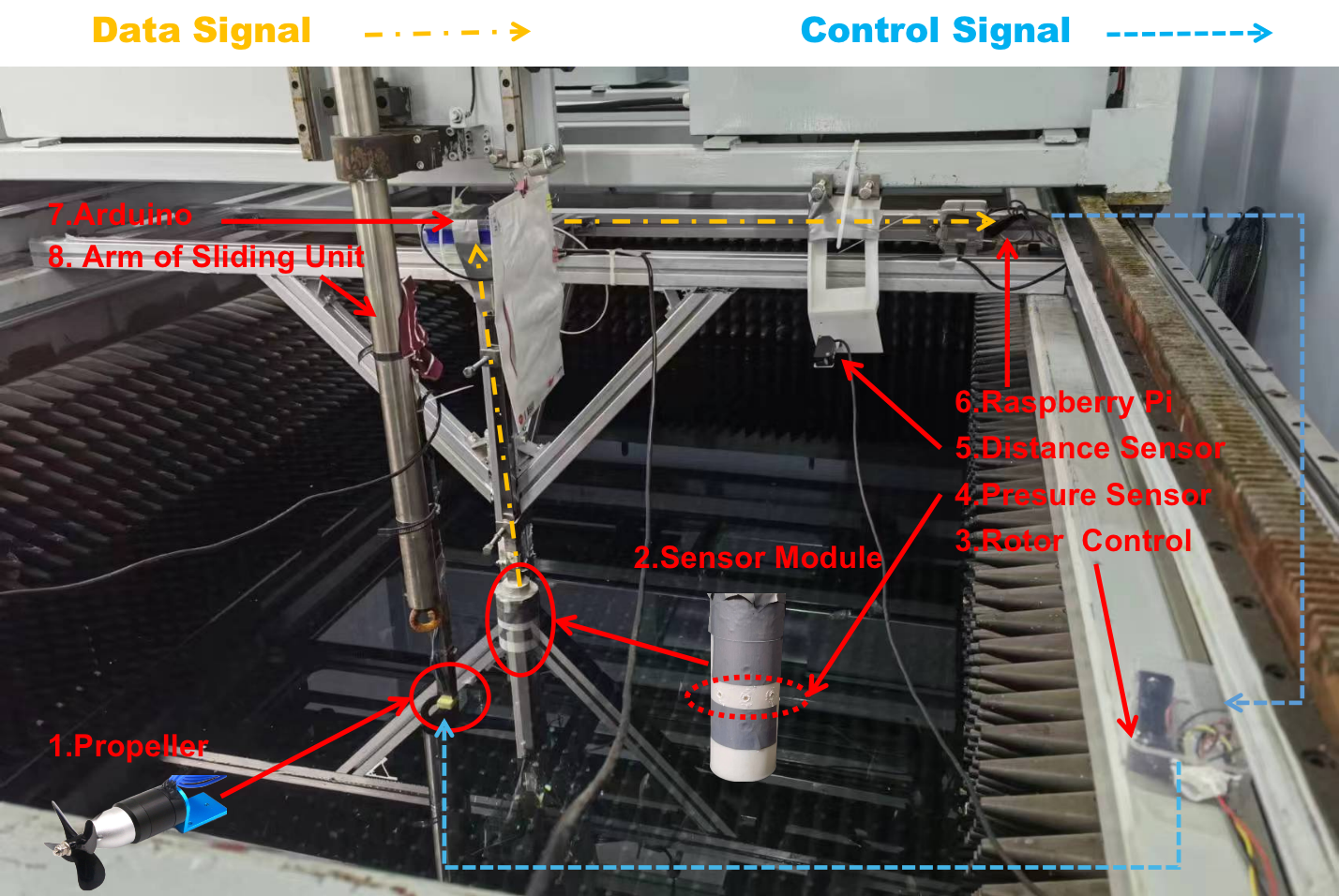
Figure 2: The designed testing platform that comprises a water tank, a sliding guide, a leader propeller, and an ALL.

Attached to the sliding guide are a data acquisition system and a leader propeller system. The data acquisition system comprises an ALL equipped with three pressure sensors and a microcomputer. A circular shaped cross-section is widely used in ALL flow sensing for its corresponding tractable hydrodynamic properties. This paper adopts the same circular shape design for the ALL (Fig. 2). The cylindrical ALL has a radius of 4 cm and a height of 20 cm. Three through-holes with a diameter of 4 mm are evenly placed for holding pressure sensors with an angle of 45 degrees between each adjacent pair at the same horizontal level of 10 cm from the bottom of the cylindar. The pressure sensors used are MS5837-02Ba, featuring a resolution of 1 Pa and I2C bus communication. To acquire multiple sensors simultaneously in real time, an TI TCA9548 eight-channel bidirectional transfer switch is used.

To accurately measure the positional states of the leading propeller, we installed a high-precision laser ranging sensor (LGKG Co HG-C1400-P). This ranging sensor features a measurement range of 0-400 mm and an accuracy of 0.8 mm with an output frequency of 100 Hz. The outputs of the ranging sensors and the ALL pressure sensors are acquired by an Arduino micro-controller that synchronizes all the signals and sends all the real-time data to the host computer, a Raspberry Pi 4 Model B with 8G memory that operates in Linux (Ubuntu 18.04) a Python program for data acquisition, processing and storage.

II-B Estimation Problem

Taking the assumption that the rotating axis of the leader propeller and all the pressure sensors of the ALL locate in the same horizontal plane, we project the propeller and the ALL onto that horizontal plane. The ALL is represented by a circle under the projection and the three sensors are represented by three points on the circle. We define a reference frame $I$ within the horizontal plane, the center of the circle as the origin $O$, and the axis pointing from the origin to the center pressure sensor as the $y$-axis. The $x$-axis is perpendicular to the $y$-axis pointing to the left. In experiment, the rotating axis of the propeller is kept parallel to the $y$-axis. The displacement of the propeller with respect to the origin is denoted by $(x,y)$ where $x$ and $y$ represent the lateral and longitudinal displacements of the leader propeller, respectively. We denote the speed of the propeller’s lateral motion along the $x$-axis by $v$, and the corresponding direction of the motion by the boollean-type varaible $d=\{\mathrm{P\ or\ N\}}$ indicating the positive or negative direction along the $x$-axis. The lateral motion states of the propeller, denoted by $\boldsymbol{s}$, include three variables, i.e., $\boldsymbol{s}=\left[x,v,d\right]^{\mathrm{T}}$. The measurement of the ALL distributed pressure sensors at time $k$ is defined as $\boldsymbol{m}_{k}\in\mathbb{R}^{N}$ where $N$ represents the number of the ALL pressure sensors. With the distributed pressure sensors measuring their corresponding local pressures in the propeller wake, the objective is to design a flow-sensing algorithm represented by function $f$ such that

$$\lim_{k\to\infty}\left|\hat{\boldsymbol{s}}_{k}-\boldsymbol{s}_{k}\right|=0$$ (1)

where $\hat{\boldsymbol{s}}_{k}=f(\boldsymbol{m}_{k})$ calculates the estimated motion states $\hat{\boldsymbol{s}}$ using the ALL pressure measurements $\boldsymbol{m}_{k}$.

III Dataset Construction

III-A Data Acquisition

We conduct extensive experiments using the aforementioned testbed to create a dataset of the ALL measurements given selected lateral motion states of the leader propeller. To eliminate the influence of the submerged depth of the pressure sensors, all the sensor outputs are debiased by deducting the corresponding pressure readings sampled before the rotation of the propeller when the flow is stationary. In each experimental trial, the leader propeller moves along the lateral axis or the $x$-axis at a constant speed $v$ with motion direction $d\in\{N,P\}$ while the longitudinal displacement $y$ is kept constant. We select five representative speeds of the moving propeller, i.e., $v\in\{400,500,600,700,800\}$ mm/s. In each trial, the sliding guide accelerates the propeller from at rest to the selected speed $v$ and keeps it at that constant speed. Considering the effective measurable width of the propeller wake by the ALL and the influence of the transient during the propeller accelerating period, the lateral motion of the propeller goes from $x=-175$ mm to $x=175$ mm and then back to $x=-175$ mm. The effective estimation range is clipped to $x\in[-120,120]$ mm and normalized in the following sections for the convenience of presentation. In addition, two longitudinal displacements are selected in the experiment, i.e., $y\in\{250,300\}$ mm.

The back-and-forth trip is repeated 10 times for each set of motion state configurations.

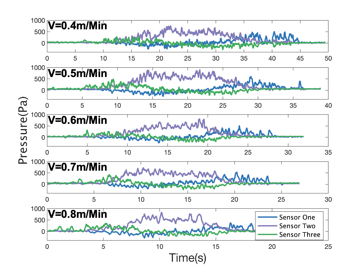
(a) Positive direction of motion or $d=P$.

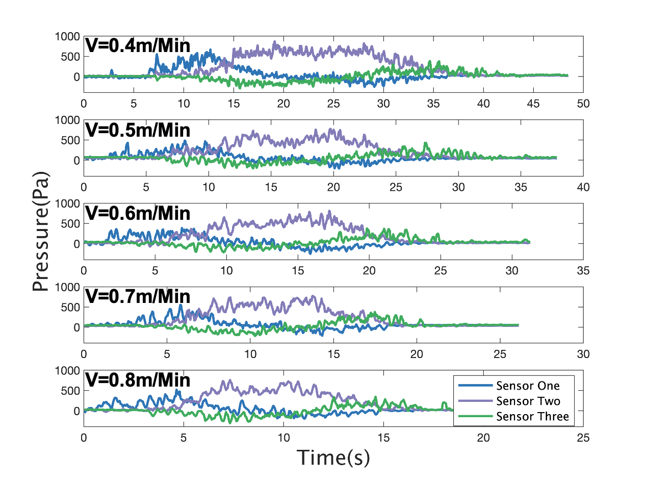
(b) Negative direction of motion or $d=N$.

Figure 3: The trajectories of pressure sensor data collected by the ALL in the experiment when the leader propeller moves laterally at different speeds.

Figure 3 shows the collected distributed pressure data given selected speeds and directions of the leader propeller. We observe strong correlations between time-domain features of the pressure measurements and the lateral motion states of interest. Specifically, the changing trends of the collective pressure measurements are primarily correlated to the direction of motion of the leader propeller; the changing rates of the pressure measurements are mainly correlated to the traveling speed of the propeller; and the magnitudes of the pressure measurements are mainly correlated to the lateral displacement of the propeller. Such observations indicate that the ALL pressure measurements of the propeller wake (most likely) contains sufficiently rich information for the estimation of the lateral motion states of the leader propeller, supporting our previous hypothesis.

III-B Time Series Selection

Most existing flow sensing studies using ALLs deal with structured flow fields such as the Von Karman vortex street of laminar flow passing a cylinder or periodic wake flow of an undulating fish-like fin. This paper, however, targets the propeller wake which features cross-scale dynamic and unstable flow structures, thus making the flow sensing problem extremely challenging. Due to the practical limitation of sampling frequency and sampling resolution of the All, it is infeasible to accurately capture all the characteristics of the propeller wake. Additionally, the phase averaging approach commonly adopted in propeller wake analysis requires the data sampling to occur at uniform phases of the periodic rotation of the propeller, which exceeds the sampling capability of almost all the ALL sensing systems. Through high-fidelity CFD simulation, we find that during the motion of the propeller, there exist a stochastic pulsation process in the ALL pressure output along with statistically distinguishable trends corresponding to different motion configurations. Therefore, we hypothesize that the time series of ALL measurement data provides partial but sufficient information regarding the lateral motion of the propeller of interest. Furthermore, increasing the number of sensors and/or the total sampling time leads to added information acquired, enhancing the robustness of the flow sensing algorithm, which poses a balancing problem between the practical engineering considerations (e.g., the cost, the installation space and real-time calculation) and the estimation accuracy. Specifically, we define the time series of the $i$-th pressure sensor output at time $k$ used for wake flow sensing as

$$\boldsymbol{M}_{k}=\left[\boldsymbol{m}_{k-sl+1},...,\boldsymbol{m}_{k}\right]^{\mathrm{T}}$$ (2)

where $\boldsymbol{m}_{k}\in\mathbb{R}^{N}$ represents the distributed pressure readings at time $k$, and $sl$ represents the sequence length of the time series. The sequential data $\boldsymbol{M}_{k}$ continuously evolves with upcoming sensory measurements embedding the flow dynamics information of the latest $sl$ time steps, forming the dataset of the time series of the ALL distributed pressure measurements for algorithm training and testing.

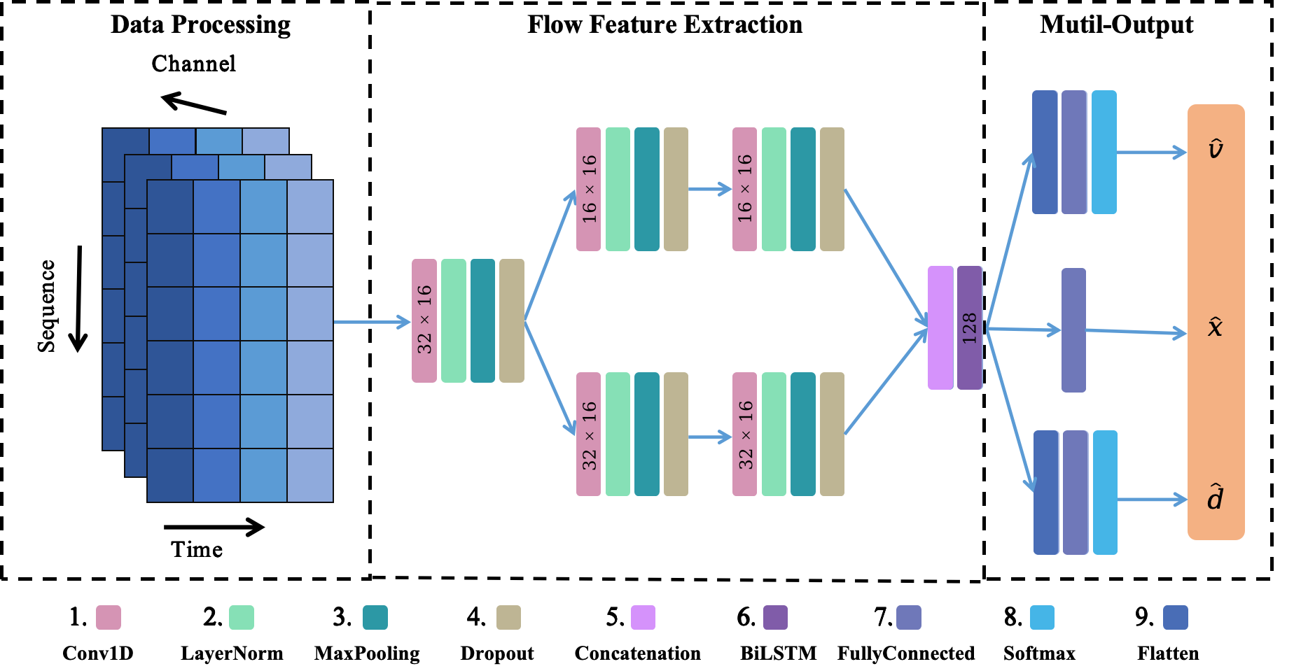
Figure 4: The schematic of the network architecture of the proposed wake flow estimator that consists of a hybrid CNN-BiLSTM network for flow feature extraction and a multi-output neural network for motion state regression and classification.

IV Motion State Estimation via Wake Sensing

IV-A Flow Feature Extraction with Hybrid CNN-BiLSTM

Considering the highly complex and stochastic dynamics of propeller wake, we adopt the trending powerful deep learning approach to extract hidden spatiotemporal flow features given the time series of the distributed ALL measurements and design a hybrid function of the one-dimension convolutional neural network (1DCNN) and the bidirectional long short-term memeory network (BiLSTM). Specifically, as one of the most widely used networks[27, 28], 1DCNN is selected to extract hidden spatial features of the sequential pressure measurement data supported by sparse connections and weight sharing. The network design consists of four main layers including the input, the convolutional, the batch normalization, and the pooling (Fig. 4). On the other hand, BiLSTM is a special recurrent neural network (RNN)[29, 30] which introduces a gate mechanism to control both the forward and reverse information transmission paths, rendering BiLSTM a stronger learning ability for long-range dependency compared to traditional RNNs[29]. In this paper, the BiLSTM network follows 1DCNN and learns the bidirectional sequential relationship from the extracted spatial features, thereby providing long-term characteristics of the time series of ALL data sampled from the unsteady and complex wake flow of the leader propeller.

Figure 4 shows the network architecture of the designed hybrid CNN-BiLSTM model. Firstly, the time series of distributed sensor data is input into a multi-channel 1DCNN where feature extraction and dimension reduction are conducted through the convolution and pooling operations. Next, the output of the 1DCNN network is fed into the BiLSTM network[31, 32] whose forgetting, input, and output gates are optimized via iterative training to learn the time-domain relationship between spatial features extracted by the 1DCNN network. Therefore, the hybrid 1DCNN-BiLSTM network extracts spatiotemporal features of the sampled wake data, expectedly providing sufficient information for estimating the lateral motion states of the leader propeller.

IV-B Motion State Estimator

Design of the loss function. This paper focuses on the estimation of the lateral motion states of the leader propeller including the relative displacement $x$, travelling speed $v$, and direction of motion $d$. Considering the properties of the motion states, we model the estimation task as a combination of regression and classification problem with continuous estimation state space of displacement $\mathcal{X}$ and discretized estimation state space of travelling speed $\mathcal{V}$ and Boolean-type direction $\mathcal{D}$. Correspondingly, we design a multi-output neural network as the motion state estimator that takes the wake flow features as input and estimates the lateral motion states of the leader propeller utilizing parameter sharing [33]. The network architecture of the designed multi-output model is depicted in the right column of Fig. 4. Given sufficiently rich experimental data, the key to the design of the state estimation model lies in the design of the loss function [34]. Considering the continuous and discrete motion states to be estimated, we first design three individual loss functions for the three estimation states, respectively. Specifically, the relative lateral displacement $x$ is estimated by regression, with its loss function $l_{1}$ designed as the mean square error loss (MSE), i.e.,

$$l_{1}=\frac{1}{N}\sum_{i=1}^{N}\left(\hat{x}-x\right)^{2}$$ (3)

where $x$ and $\hat{x}$ represent the actual and the estimated displacements, respectively. Modeled as discrete states, the speed $v$ and the direction of speed $d$ are estimated via classification with their loss functions $l_{2}$ and $l_{3}$ designed using the cross-entropy loss, i.e.,

$$l_{2}=-\frac{1}{N}\sum_{i}^{N}\sum_{k=1}^{V}z_{ik}\log\left(p_{ik}\right)\\$$ (4)

$$l_{3}=-\frac{1}{N}\sum_{i}^{N}\sum_{k=1}^{D}z_{ik}\log\left(p_{ik}\right)$$ (5)

where $N$ is the size of the sampling batch, $V$ and $D$ are the numbers of categories or the discretization levels of the speed and direction of motion, respectively, boolean-type $z_{ik}$ denote whether sample $i$ belongs to category $k$ (1 for yes and 0 for no), $p_{ik}$ denotes the predicted probability that the observed sample $i$ belongs to category $k$.

Designed as a linear combination of the three individual losses, the overall loss function of the state estimator calculates as follows

$$l=\lambda_{1}l_{1}+\lambda_{2}l_{2}+\lambda_{3}l_{3}$$ (6)

where the task weight $\lambda_{i}$ balances the relative importance between the three estimated states. The multiple output model utilizes the feature extraction module with parameter sharing.

Optimizing task weights. Considered as a multi-objective optimization problem, the selection of the weights $\lambda_{i}$ where $i\in\{1,2,3\}$ greatly affects the overall estimation performance. In this paper, a nature inspired meta-heuristic optimization algorithm named the whale optimization algorithm (WOA) is used to search for the optimal weights $\lambda_{i}$. Proposed by Mirjalili et al. in 2016[35], WOA mimics the hunting behavior of humpback whales in their bubble-net predation, featuring the advantage of less parameters to tune and easiness to implement. The primary process of the algorithm consists of three essential stages including encircling prey, feeding with bubble nets, and finding prey[36]. To optimize the task weights, we design a performance evaluation vector $\boldsymbol{e}=[1-\text{ACC}_{1},1-\text{ACC}_{2},\text{ERR}]$ where $\text{ACC}_{1}$ and $\text{ACC}_{2}$ represent the state estimation accuracy of the lateral motion speed $v$ and the direction of motion $d$, respectively, and ERR represents the mean square error of the estimated displacement $x$. The optimization fitness $g$ (or the cost) is then designed as 1-norm of the performance evaluation vector $\boldsymbol{e}$, i.e.,

$$g(\lambda_{1},\lambda_{2},\lambda_{3},)=\|\boldsymbol{e}\|_{1}$$ (7)

Searching for the minimum of the fitness over the task weight space, WOA optimizes the overall estimation performances. Specifically, WOA first initializes the task weights $\lambda_{i}$ and the WOA algorithm parameters such as the searching agent population and the maximum iteration number. Next, given the wake flow dataset constructed in Section III, WOA computes the fitness $g$ for each searching agent and updates the position of each agent accordingly. Repeat the step until conditions are met such as parametric convergence obtained or maximum iteration steps reached.

IV-C Hyperparameters and Training Environment

Hyperparameters are the tunable training parameters that directly affect the learning results of the estimation network model. In this paper, the batch size is set to 64, the learning rate is set to $1\times 10^{4}$, and the number of epochs is set to 200. Adam’s algorithm is used for optimization. Adopting softmax output, the classification task categorizes the direction of motion into two classes and the lateral speed of the propeller into five classes. The regression task adopts a fully connected network output normalized to the interval [-1,1]. To avoid overfitting, the dropout technique is utilized. The model training and testing are conducted on a desktop computer with the configuration of an Intel 12900K CPU, an Nvidia RTX 3080 Ti GPU, and a 64GB RAM.

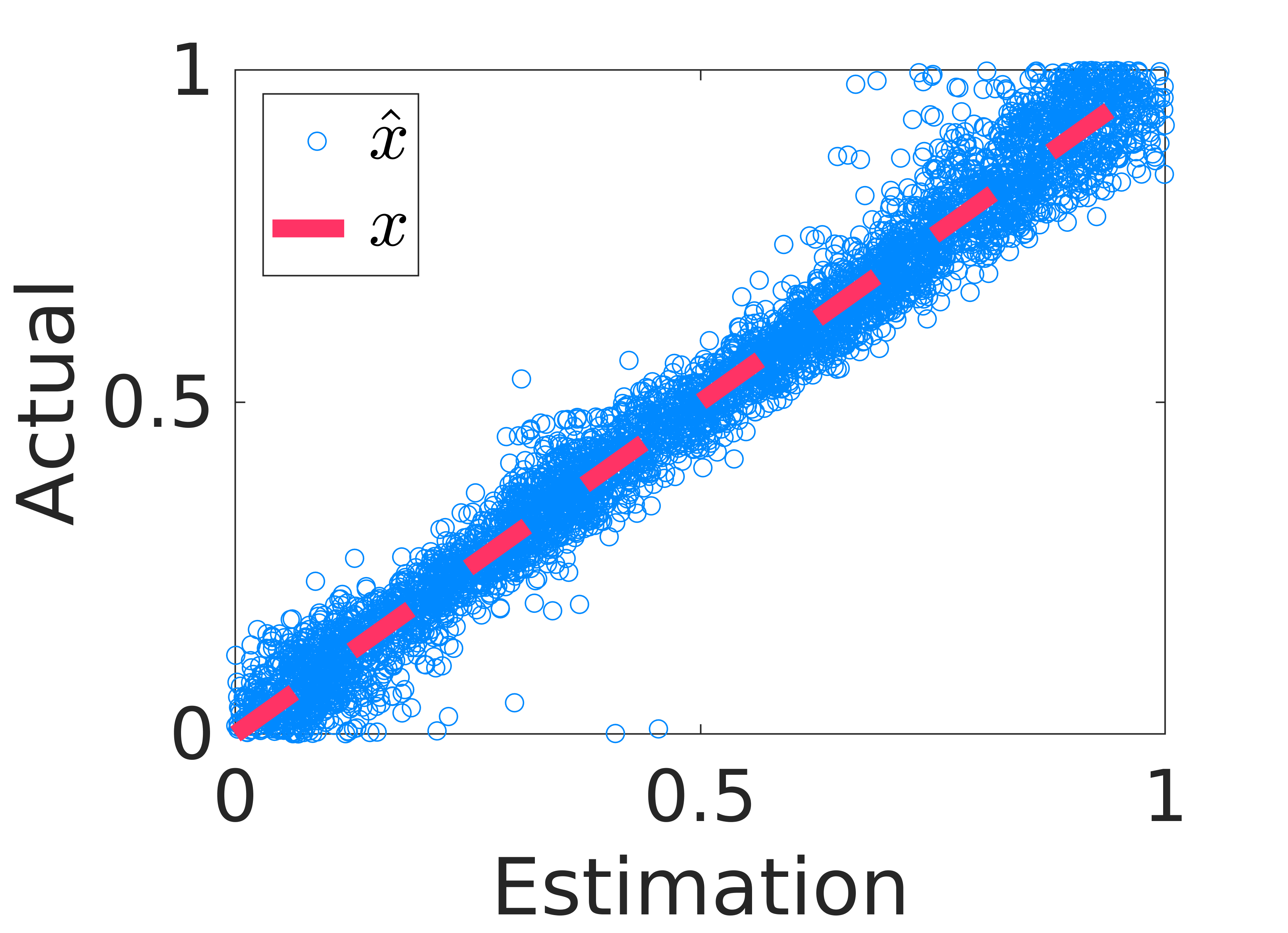
(a) Lateral displacement $\hat{x}$ in Case 1.

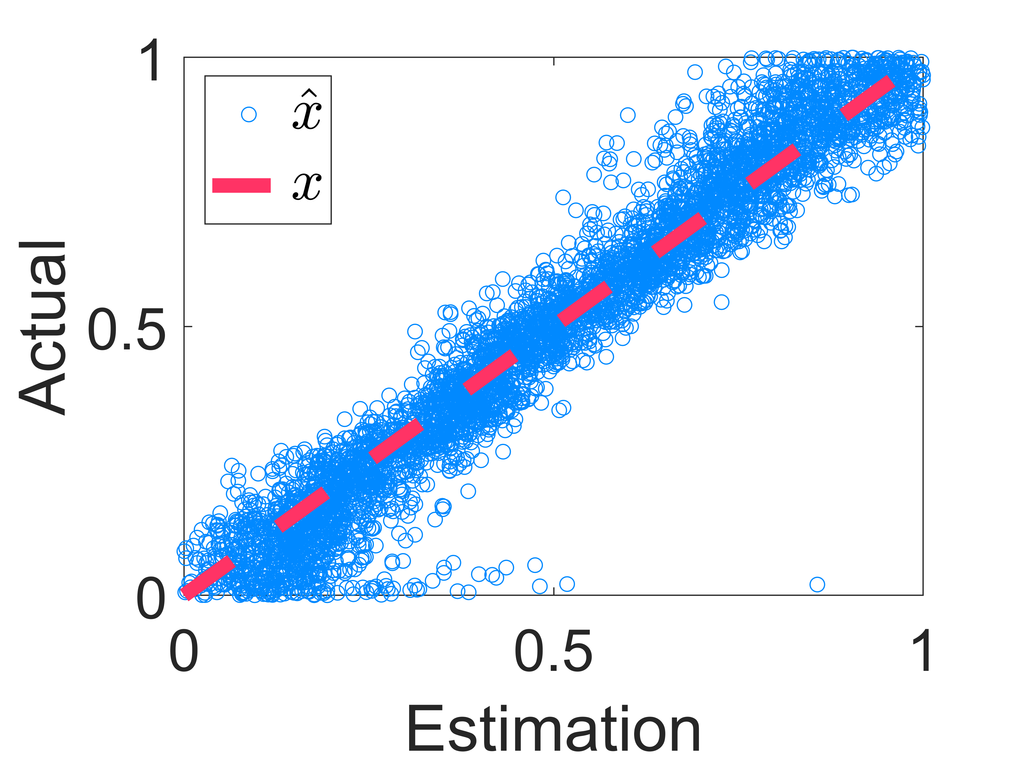
(b) Lateral displacement $\hat{x}$ in Case 2.

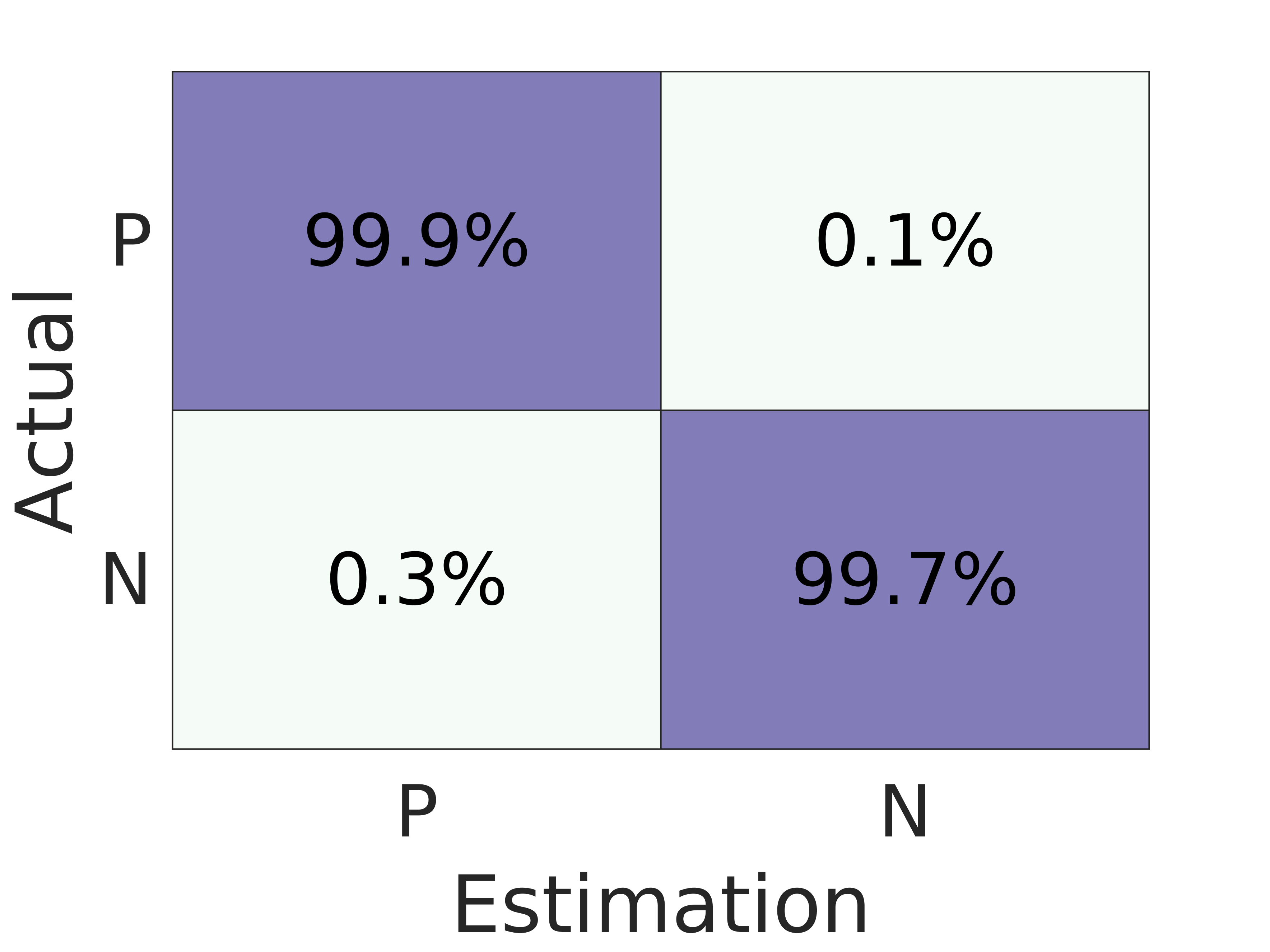
(c) Confusion matrix of direction of motion $\hat{d}$ in Case 1.

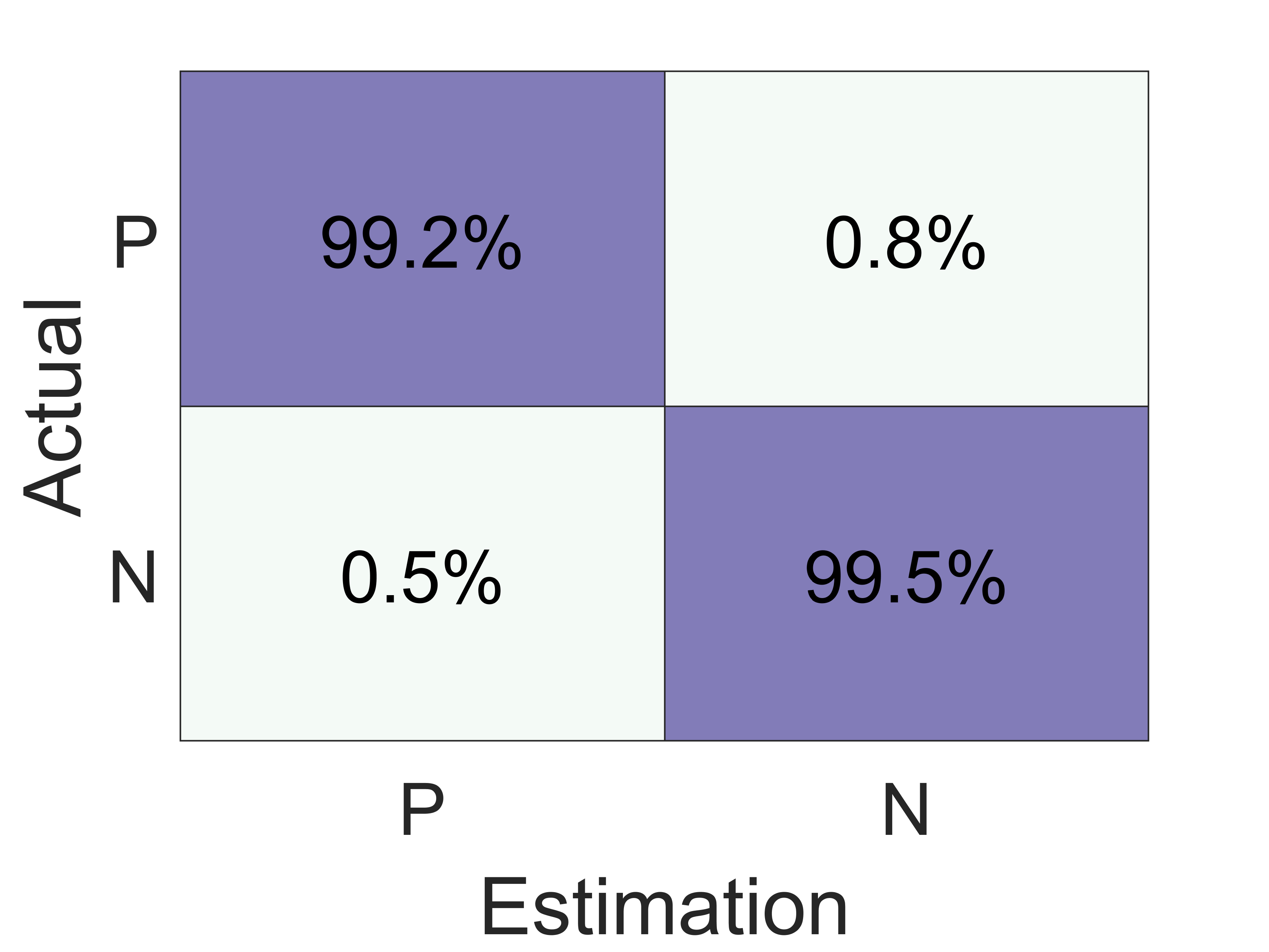
(d) Confusion matrix of direction of motion $\hat{d}$ in Case 2.

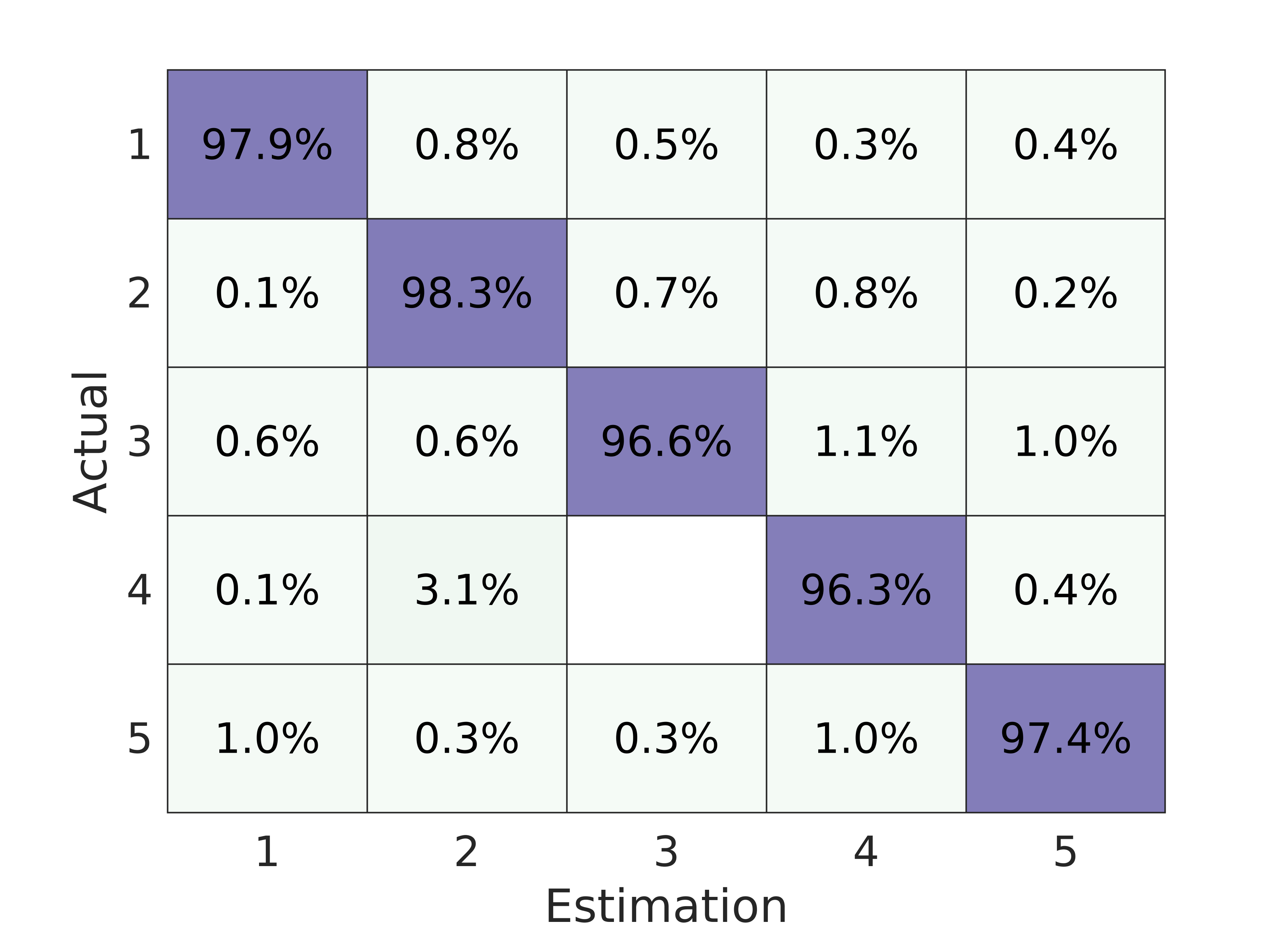
(e) Confusion matrix of traveling speed $\hat{v}$ in Case 1.

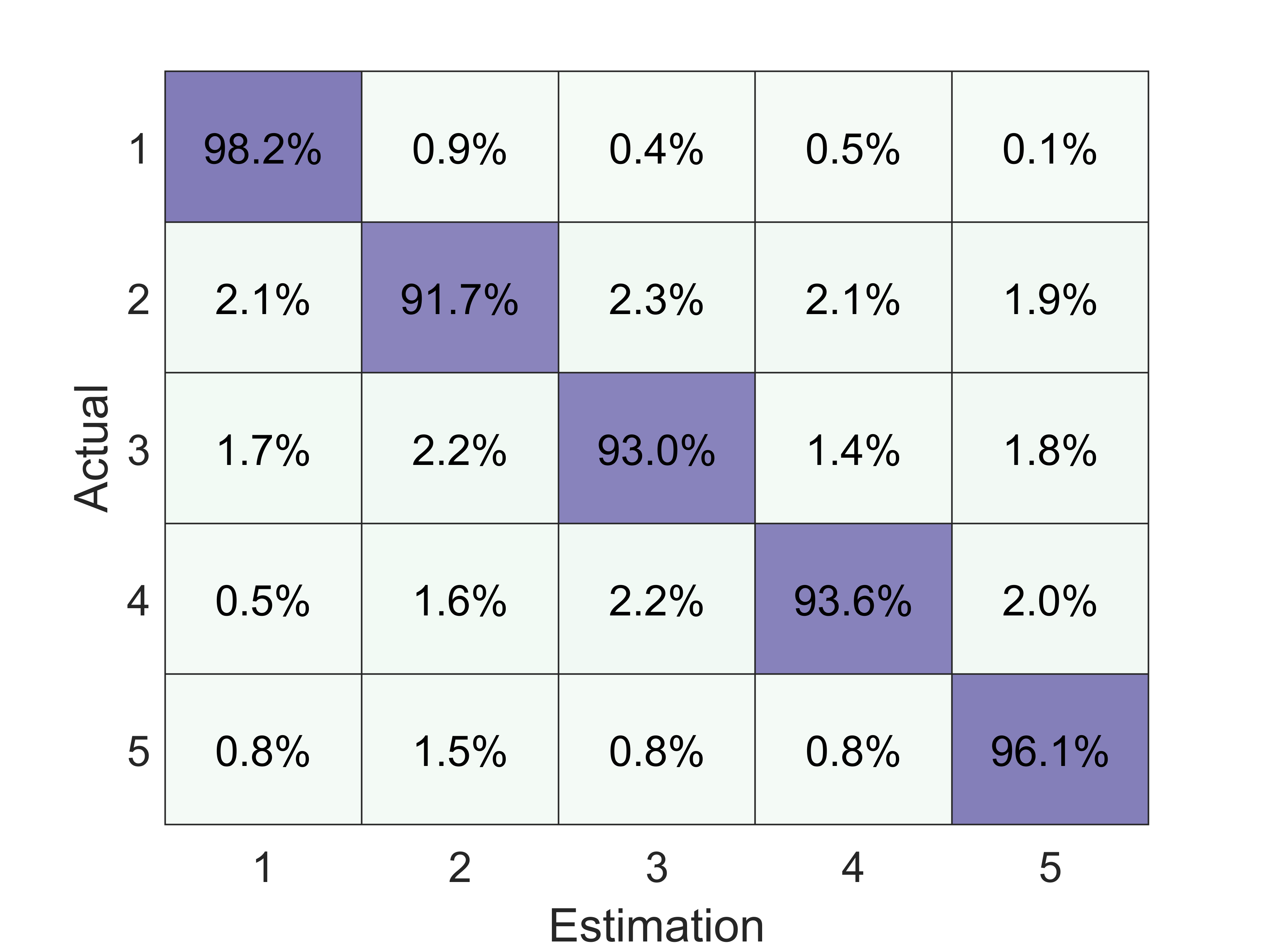
(f) Confusion matrix of traveling speed $\hat{v}$ in Case 2.

Figure 5: The experimental results of the motion state estimation based on propeller wake sensing including specifically the regression results on the lateral displacement $x$, and the classification results on the traveling speed $v$ and the direction of motion $d$.

IV-D Experimental Results

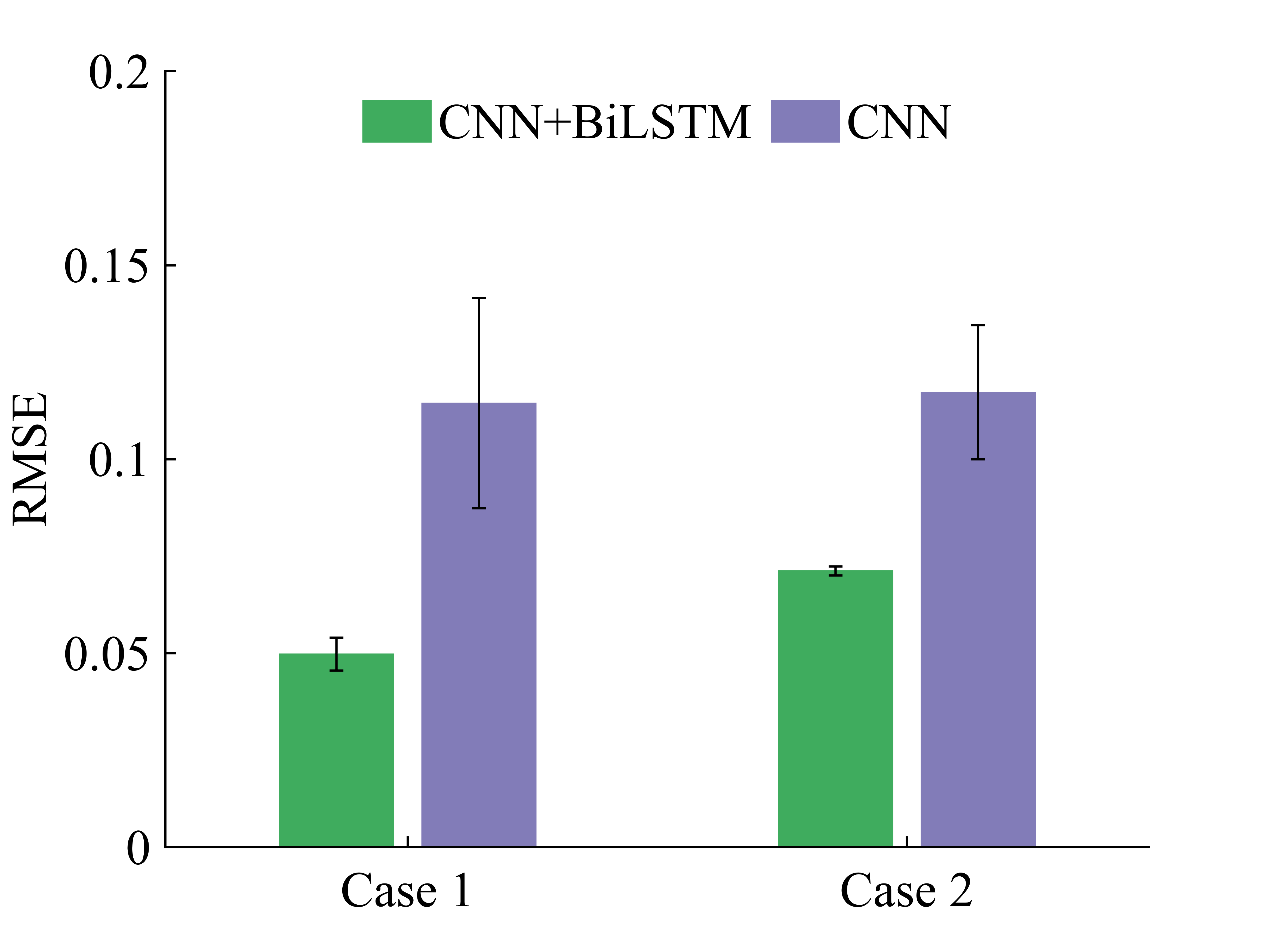
(a) Lateral displacement estimate $\hat{x}$.

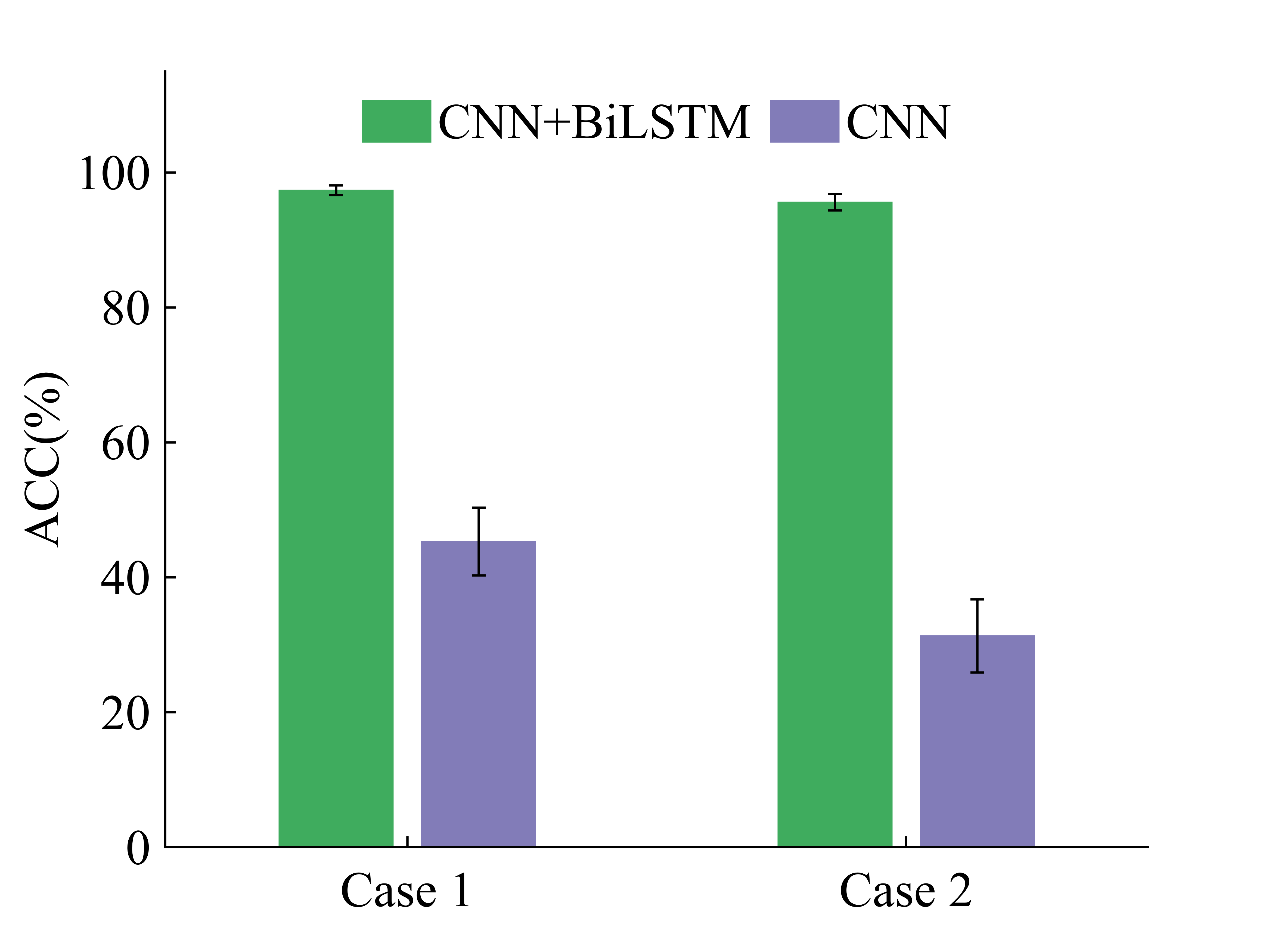
(b) Traveling speed estimate $\hat{v}$.

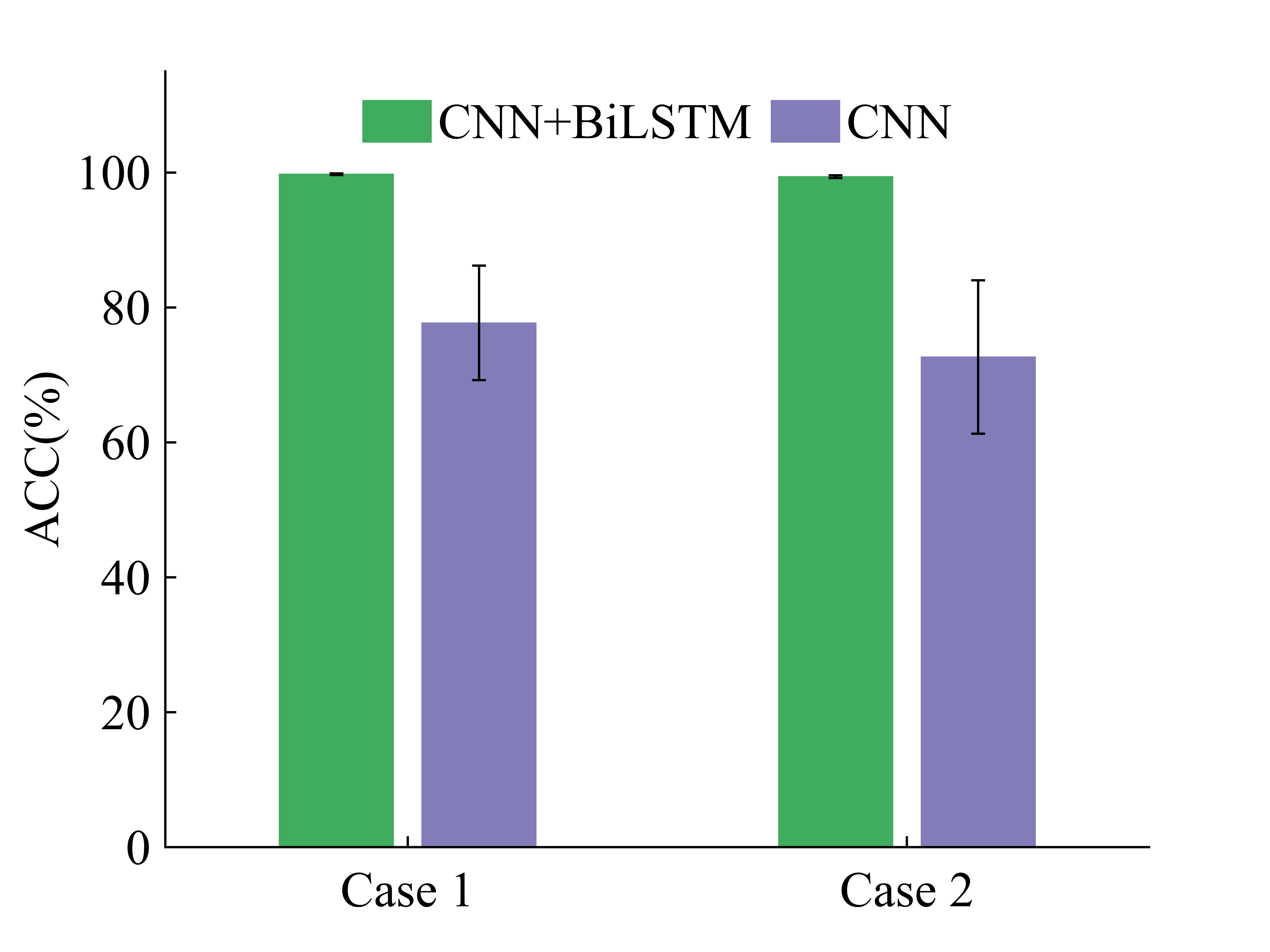
(c) Direction of motion estimate $\hat{d}$.

Figure 6: The experimental results of motion state estimation comparing the proposed hybrid CNN-BiLSTM model and the commonly-used CNN model. The adopted performance evaluation metrics are the RMSE for the lateral displacement and the ACC for the traveling speed and direction of motion.

To demonstrate the effectiveness of the proposed motion state estimation method, experiments are designed and conducted. Two longitudinal displacements $y\in\{250,300\}$ mm are adopted and tested for each experimental configuration as comparative studies pertaining to the separation distance between the ALL sensing system and the leader propeller. The two longitudinal displacements of $250$ mm and $300$ mm are referred to as Case 1 and Case 2 in the following sections for the convenience of discussion. The length of the sliding window $sl$ is set to $64$. The training and testing data follow a 9:1 ratio division.

Figure 5 shows the experimental results of the lateral motion state estimation of the leader propeller. Table I presents the statistical estimation results for each motion state over all the experimental tests in Case 1 and Case 2, respectively. Specifically, Figs 5(a) and 5(b) show the estimates and the actual values of the lateral displacement of the traveling leader propeller for Case 1 and Case 2, respectively. The red dashed line represents perfect estimation for reference; the blue circles represent the state estimates $\hat{x}$. The experimental results show that the estimated displacements are generally close to the actual value indicating a good regression performance. Furthermore, Table I reveals that a larger longitudinal displacement leads to a slightly increased root mean square error (RMSE) at 0.07 compared to that of 0.05 from the smaller longitudinal displacement. Meanwhile, the standard deviation of the estimation error from both cases are satisfactorily small at 0.0042 and 0.0012, respectively. Figures 5(c)-5(f) show the estimation results regarding the travelling speed ${v}$ and the direction of motion ${d}$ of the leader propeller represented by the confusion matrices that demonstrate the classification performance. The rows and the columns of the confusion matrix correspond to the actual and predicted classes, respectively. The diagonal and off-diagonal elements correspond to the true and false observation results, respectively. Figures 5(c) and 5(d) illustrate the estimation performance regarding the direction of motion ${d}$. $P$ and $N$ represent along the positive and negative $y$-axis directions, respectively. It is observed that the accuracy of the direction state classification is greater than 99.5% for the smaller longitudinal displacement $y=250$ mm while the accuracy is greater than 99% for the larger longtudinal displacement $y=300$ mm. The RMSE is less than 0.2% for both the cases. Specifically, Figures 5(e) and 5(f) illustrate the estimation performance regarding the traveling speed ${v}$ where 5 different lateral speeds of $0.4,0.5,0.6,0.7,0.8$ m/min are used corresponding to the first to the fifth columns of the confusion matrix labeled as $1$ to $5$. We observe that the accuracy of the lateral speed classification is consistently greater than 91% with a mean square error less than 1.5%.

TABLE I: The experimental results of the statistical estimation performance for all the three motion states in Case 1 and Case 2 using both optimized and random task weights.

Case	RMSE of $\hat{x}$	ACC1 of $\hat{v}$	ACC2 of $\hat{d}$
Case 1 (with Optimization Parameters)	0.0498$\pm$ 0.0042	97.37$\pm$0.72%	99.75$\pm$0.11%
Case 1 (with Random Parameters)	0.0661$\pm$ 0.0120	93.47$\pm$7.32%	98.31$\pm$1.86%
Case 2 (with Optimization Parameters)	0.0712$\pm$ 0.0012	95.58$\pm$1.21%	99.37$\pm$0.21%
Case 2 (with Random Parameters)	0.0645$\pm$ 0.0159	89.16$\pm$24.23%	98.89$\pm$1.9%

The satisfactory experimental results validate the proposed motion state estimation algorithm, which further indicate that the propeller wake features extracted from the ALL distributed pressure measurements are sufficiently rich for estimating the motion states of a leader propeller-driven underwater robot in a leader-follower formation.

IV-E Ablation Study

Ablation experiments are conducted to verify the proposed hybrid CNN-BiLSTM design in feature extraction. Specifically, the BiLSTM network is removed with only the CNN model left as the comparison. The comparison experimental results are shown in Fig. 6 in terms of the three estimated states, i.e., the lateral displacement $x$, the lateral speed $v$, and the direction of motion $d$ of the leader propeller. The green bars represent the mean of the estimates using the proposed CNN-BiLSTM model while the purple bars represent the mean of the estimates using the CNN model. The error bars represent the standard deviations of the estimates for all the three motion states of interest over all the experimental tests in Case 1 and Case 2, respectively. From the comparison results, we observe a consistent performance improvement using CNN-BiLSTM compared to CNN for all the three motion states of interest and two longitudinal displacement cases. Specifically, Fig. 6(a) shows a roughly 30% improvement in the RMSE of the lateral displacement regression. Figure 6(b) demonstrates a significantly enhanced accuracy of over 50% improvement in estimating the travelling speed of the leader propeller. Similarly, a superior performance is observed with an accuracy improvement of over 10% in estimating the direction of motion as shown in Fig. 6(c). The ablation study validates the necessity and the effectiveness of the proposed CNN-BiLSTM model particularly over the traditionally used CNN network.

V Analysis and Discussion

V-A Length of Time Series on Estimation Performance

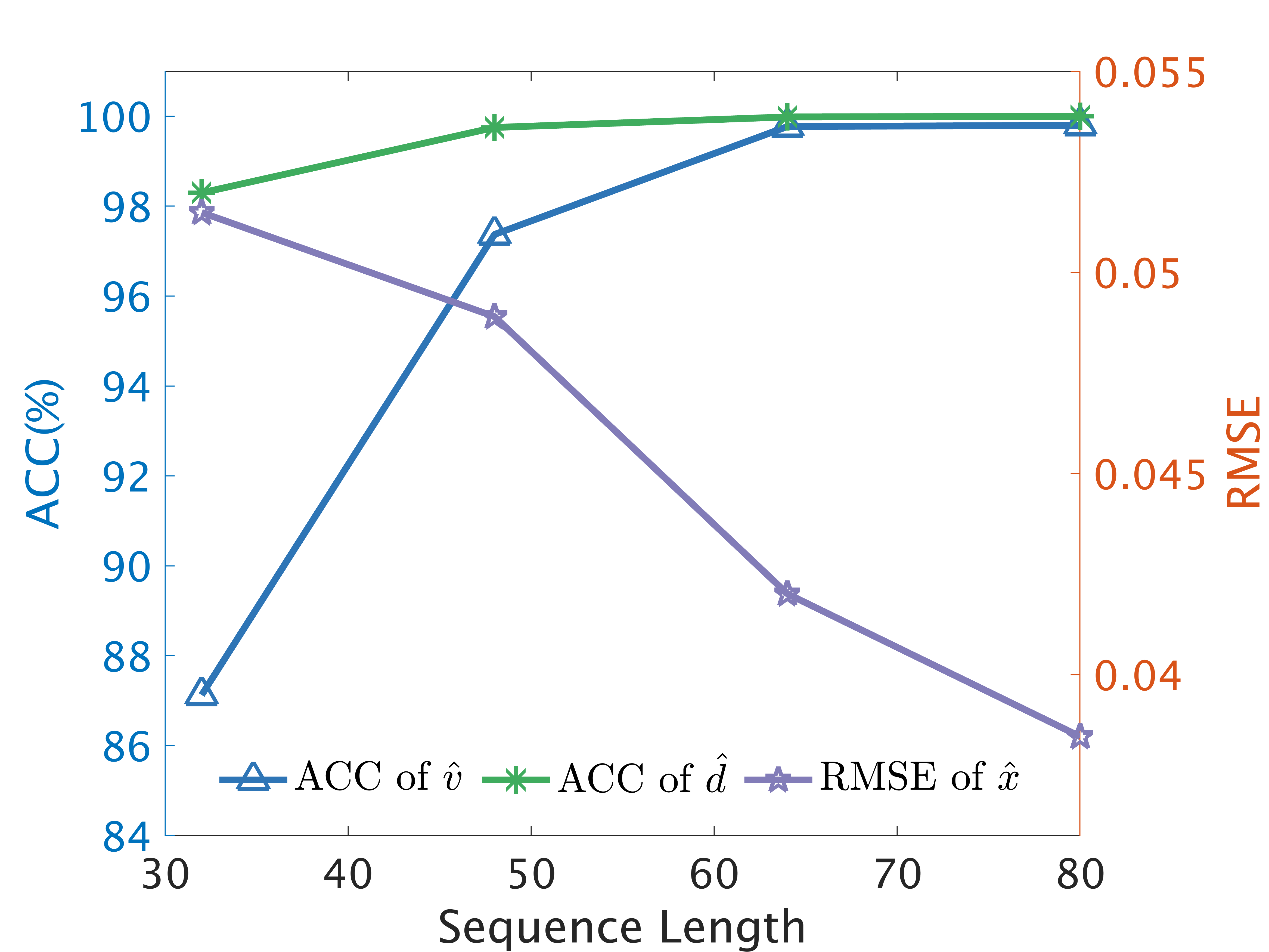
Figure 7: The experimental results of the motion state estimation performance with respect to the sequence length of the time series used in the estimation algorithm. Specifically, the estimation performance ACC of $v$ and $d$ uses the axis scale on the left, and RMSE of $x$ uses the axis scale on the right.

Time series of the ALL pressure measurements are used to capture the dynamics of the propeller wake in this paper. Intuitively, the sequence length of the time series is critical in the extraction of the dynamic flow features. Studies are conducted to further investigate the influence of the sequence length on the estimation results, aiming to provide insights into the relationship between required data length and the motion states of the leader propeller. Experimental data collected at longitudinal displacement $y=250$ mm is used while all the other parameters are kept the same as in aforementioned experiments. The sequence lengths of the pressure measurement data for comparative analysis in the estimation algorithm are selected to be $sl=[32,48,64,80]$.

Figure 7 shows the experimental results of the influence of the time-series sequence length on the estimation performance represented by the corresponding evaluation metrics. Specifically, the classification accuracy (ACC) for the traveling speed $v$ and the motion of direction $d$ follows the axis scale on the left hand side, and the regression root mean square error (RMSE) for the lateral displacement $x$ follows the axis scale on the right hand side. We observe that as the sequence length increases, the RMSE of the lateral displacement decreases slightly indicating a gentle performance improvement. On the other hand, the classification accuracy of both the travelling speed and the motion of direction increases considerably when the sequence length increases. Overall, the longer length of the time-series is used in the estimation algorithm, the higher the motion estimation performance is achieved, which we conjecture comes from the extra flow dynamics information embedded in the added sampled data. However, longer sequence length leads to more time delay in the estimation process, thus possibly hindering real-time control tasks. Comprehensively considering the estimation performance and the real-time requirement of the ALL sensing system, the selection of the sequence length of the sensor measurement time series is expected to be resolved with respect to different applications. Particularly, $sl=64$ is adopted in this paper.

V-B Optimized Task Weights on Estimation Performance

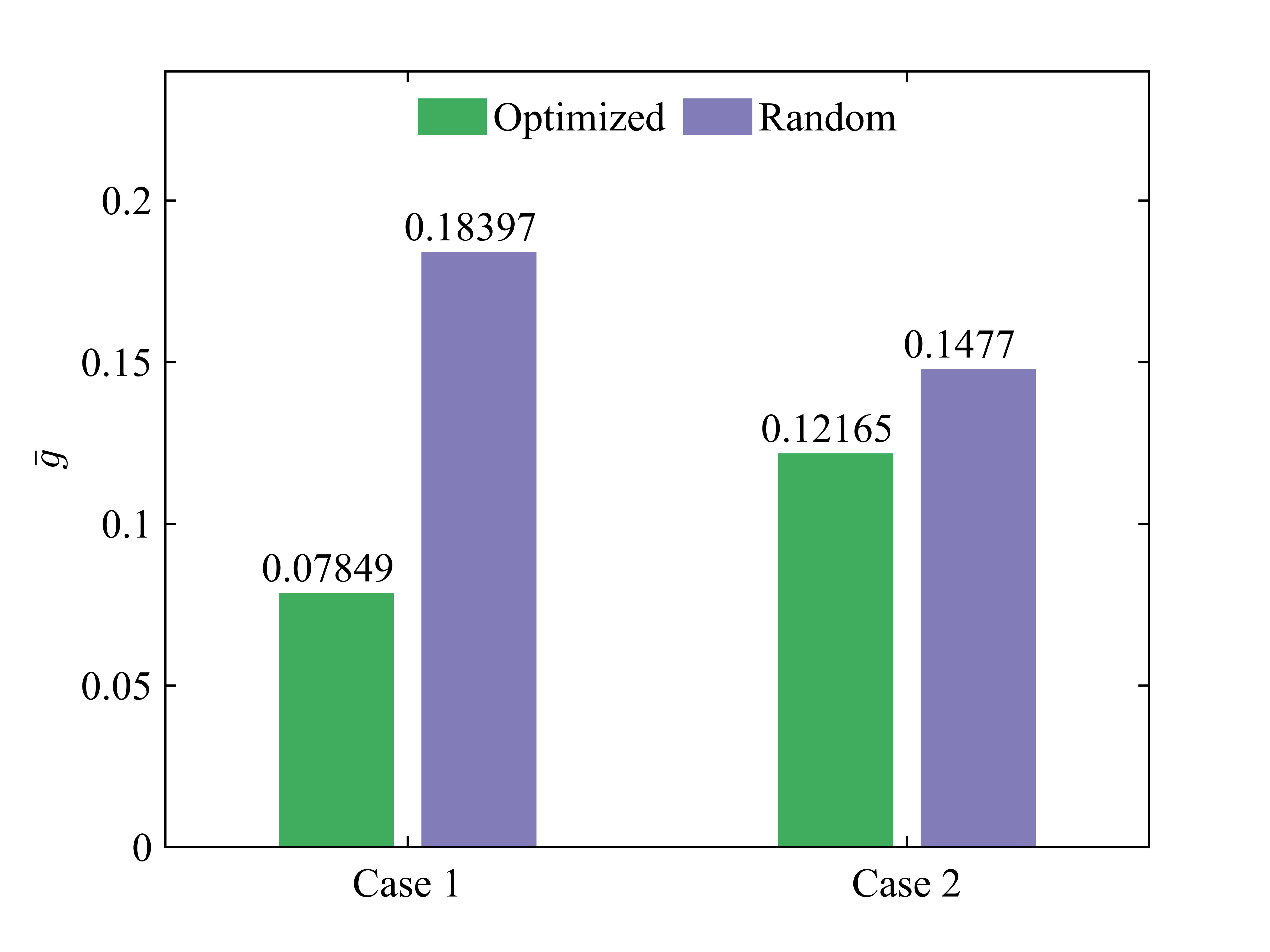
Figure 8: The comparative experimental results of the statistical fitness $g$ between using optimized and random task weights in Case 1 and Case, respectively.

The loss function $l$ in Eq. (6) designed for training the estimator network is a linear combination of the corresponding performance loss for the estimation tasks regarding the three motion states of interest with weight $\lambda_{i}$ as the design parameters. Formulated as a multi-objective optimization problem for the multi-state estimation, a biomimetic algorithm WOA is adopted to find the optimal task weight $\lambda_{i}$. This section conducts comparative experiments between using the optimized weights and using random weights, aiming to shed light on the influence of the weight optimization on the overall estimation performance. The comparative experimental results are shown in Fig. 8 and Table I. From Fig. 8, we observe that the fitness $g$ with optimized weights in Eq. (7) is significantly reduced by roughly 57% and 17% in Case 1 and Case 2, respectively. To further analyze the difference between optimized weights and randomly generated weights, comparative experiments are repeated 10 times for 10 selected trained estimation models. Table I shows the statistical results of the evaluation performances. The first and third rows are the estimation results using the optimized weights and the second and fourth rows use randomly generated weights. From Table I, we observe an estimation accuracy improvement by 4% for the speed $v$ and 1.4% for the direction of motion as well as an estimation accuracy improvement (RMSE) by 24.6% for the displacement $x$ in Case 1. We want to point out the estimation result on displacement $x$ in Case 2 decreases by 0.6% which comes from the highly-coupling phenomenon of the multi-objective optimization. The standard deviations of the estimation accuracy for all the three states are reduced by at least 65% with the optimized weights, indicating a more robust and consistent estimation performance over all the motion states and the testing conditions.

TABLE II: The comparison between our method and other selected methods of ALL-based state estimation of underwater robots.

	wake flow generation	multi-state estimation
MIT [14]	fishlike body undulation + caudal fin flapping	✗
PKU [37, 38, 39, 40]	robot fish tail flapping	✗
NTU [13]	robot fish tail flapping	✔
HEU [41]	robot fish body undulation	✗
UMD [42]	Joukowski hydrofoil flapping	✔
Ours	high-speed rotating propller	✔

V-C Comparison with Other Wake Sensing Methods

This section compares our proposed method with some of the existing wake sensing methods to highlight its unique contributions and advantages in the field. Table II shows the comparison results in terms of the generation method of the wake flow and whether multiple motion states are estimated simultaneously. The table refers to the selected literature by their organizations including the Massachusetts Institute of Technology (MIT)[14], Peking University (PKU)[37, 38, 39, 40], Harbin Engineering University (HEU)[41], National Taiwan University (NTU)[13], and the University of Maryland (UMD)[42]. In contrast to the existing methods that primarily focus on flow fields generated by periodic body undulation and tail flapping of bioinspired robotic fish, our study addresses the dynamic and complex wake flow generated by underwater robots propelled by high-speed rotating propellers. Meanwhile, our method provides the simultaneous estimation of multiple motion states via the multi-output network design that combines regression and classification operations. The existing studies demonstrate various important applications of ALL-based wake sensing such as hydrodynamic efficiency enhancement[14], robot formation control[39, 40, 41], and flow-relative localization[37, 38, 13, 42]. Consequently, our method holds great potential for expanding these applications to a wider range of uses in propeller-driven underwater robots.

VI Conclusions

This paper investigated the challenging problem of estimating the relative motion states of a propeller-driven leader underwater robot in the leader-follower formation. Making a hypothesis that the ALL pressure measurements provide partial but sufficiently rich information of the propeller wake of a leader underwater robot, we proposed a novel motion state estimation method that assimilated distributed pressure measurements sampled from the dynamic and complex propeller wake. Specifically, to estimate the lateral displacement, speed, and direction of motion of the leader propeller, a hybrid network that combined 1DCNN and BiLSTM was designed to extract the spatiotemporal characteristics of the flow field, followed by a multi-output network for state estimation. An experimental testbed was constructed. Extensive experimental tests were conducted, the results of which validated the proposed estimation method. Furthermore, comparative studies were conducted, providing insights into the design of the multi-objective loss function for training the estimator network as well as the selection of the sequence length of the pressure measurement time series used in the estimation algorithm.

In future work, we will apply the proposed wake flow sensing approach to investigate three-dimensional motion state estimation of a propeller-driven leader underwater robot. We also plan to integrate the estimation algorithm with feedback control design and experimentally test leader-follower formation control of propeller-driven underwater robots.

References

- [1] S. Coombs, “Smart skins: information processing by lateral line flow sensors,” Autonomous robots, vol. 11, pp. 255–261, 2001.
- [2] S. Coombs and S. Van Netten, “The hydrodynamics and structural mechanics of the lateral line system,” Fish physiology, vol. 23, pp. 103–139, 2005.
- [3] Y. Zhai, X. Zheng, and G. Xie, “Fish lateral line inspired flow sensors and flow-aided control: A review,” Journal of Bionic Engineering, vol. 18, no. 2, p. 264–291, 2021.
- [4] A. T. Abdulsadda, F. Zhang, and X. Tan, “Localization of source with unknown amplitude using ipmc sensor arrays,” in Electroactive Polymer Actuators and Devices (EAPAD) 2011, vol. 7976. SPIE, 2011, pp. 631–641.
- [5] L. DeVries, F. D. Lagor, H. Lei, X. Tan, and D. A. Paley, “Distributed flow estimation and closed-loop control of an underwater vehicle with a multi-modal artificial lateral line,” Bioinspiration & Biomimetics, vol. 10, no. 2, p. 025002, 2015.
- [6] T. Salumäe and M. Kruusmaa, “Flow-relative control of an underwater robot,” Proceedings of the Royal Society A: Mathematical, Physical and Engineering Sciences, vol. 469, no. 2153, p. 20120671, 2013.
- [7] H. Liu, K. Zhong, Y. Fu, G. Xie, and Q. Zhu, “Pattern recognition for robotic fish swimming gaits based on artificial lateral line system and subtractive clustering algorithms,” Sensors & Transducers, vol. 182, no. 11, p. 207, 2014.
- [8] F. Zhang, F. D. Lagor, D. Yeo, P. Washington, and D. A. Paley, “Distributed flow sensing for closed-loop speed control of a flexible fish robot,” Bioinspiration & Biomimetics, vol. 10, no. 6, p. 065001, 2015.
- [9] W. Yen, D. M. Sierra, and J. Guo, “Controlling a robotic fish to swim along a wall using hydrodynamic pressure feedback,” IEEE Journal of Oceanic Engineering, vol. 43, no. 2, pp. 369–380, 2018.
- [10] F. Dang, S. Nasreen, and F. Zhang, “Dmd-based background flow sensing for auvs in flow pattern changing environments,” IEEE Robotics and Automation Letters, vol. 6, no. 3, p. 5207–5214, 2021.
- [11] Y. Jiang, Z. Gong, Z. Yang, Z. Ma, C. Wang, Y. Wang, and D. Zhang, “Underwater source localization using an artificial lateral line system with pressure and flow velocity sensor fusion,” IEEE/ASME Transactions on Mechatronics, vol. 27, no. 1, p. 245–255, 2022.
- [12] J. Wang, T. Shen, D. Zhao, and F. Zhang, “Flow sensing-based underwater target detection using distributed mobile sensors,” in 2022 IEEE 61st Conference on Decision and Control (CDC). IEEE, 2022, pp. 2681–2687.
- [13] W. Yen, C. Huang, H. Chang, and J. Guo, “Localization of a leading robotic fish using a pressure sensor array on its following vehicle,” Bioinspiration & Biomimetics, vol. 16, no. 1, p. 016007, 2020.
- [14] A. Gao and M. S. Triantafyllou, “Independent caudal fin actuation enables high energy extraction and control in two-dimensional fish-like group swimming,” Journal of Fluid Mechanics, vol. 850, pp. 304–335, 2018.
- [15] B. Colvert, M. Alsalman, and E. Kanso, “Classifying vortex wakes using neural networks,” Bioinspiration & Biomimetics, vol. 13, no. 2, p. 025003, 2018.
- [16] T. Lowndes, “AUV swarms for monitoring rapidly evolving ocean phenomena,” Ph.D. dissertation, University of Southampton, 2020.
- [17] A. Amory and E. Maehle, “SEMBIO-a small energy-efficient swarm AUV,” in OCEANS 2016 MTS/IEEE Monterey. IEEE, 2016, pp. 1–7.
- [18] N. R. Rypkema, “Underwater & out of sight: Towards ubiquity in underwater robotics,” Ph.D. dissertation, Massachusetts Institute of Technology, 2019.
- [19] A. Di Mascio, G. Dubbioso, and R. Muscari, “Vortex structures in the wake of a marine propeller operating close to a free surface,” Journal of Fluid Mechanics, vol. 949, 2022.
- [20] R. Muscari, G. Dubbioso, and A. Di Mascio, “Analysis of the flow field around a rudder in the wake of a simplified marine propeller,” Journal of Fluid Mechanics, vol. 814, p. 547–569, 2017.
- [21] P. Kumar and K. Mahesh, “Large eddy simulation of propeller wake instabilities,” Journal of Fluid Mechanics, vol. 814, p. 361–396, 2017.
- [22] L. Wang, C. Guo, C. Wang, and P. Xu, “Modified phase average algorithm for the wake of a propeller,” Physics of Fluids, vol. 33, no. 3, p. 035146, 2021.
- [23] M. Heydari and H. Sadat-Hosseini, “Analysis of propeller wake field and vortical structures using k- SST method,” Ocean Engineering, vol. 204, p. 107247, 2020.
- [24] J. Gong, J. ming Ding, T. cheng Wu, J. bing Jiang, and C. yu Guo, “2d-3c piv measurement of the near wake of a ducted propeller,” Ocean Engineering, vol. 252, p. 111223, 2022.
- [25] L. Wang, J. E. Martin, M. Felli, and P. M. Carrica, “Experiments and cfd for the propeller wake of a generic submarine operating near the surface,” Ocean Engineering, vol. 206, p. 107304, 2020.
- [26] Y. Jia and L. Wang, “Leader–follower flocking of multiple robotic fish,” IEEE/ASME Transactions on Mechatronics, vol. 20, no. 3, pp. 1372–1383, 2015.
- [27] S. Kiranyaz, O. Avci, O. Abdeljaber, T. Ince, M. Gabbouj, and D. J. Inman, “1D convolutional neural networks and applications: A survey,” Mechanical systems and signal processing, vol. 151, p. 107398, 2021.
- [28] J. Koushik, “Understanding convolutional neural networks,” 2016.
- [29] S. Hochreiter and J. Schmidhuber, “Long short-term memory,” Neural computation, vol. 9, no. 8, pp. 1735–1780, 1997.
- [30] A. Graves and J. Schmidhuber, “Framewise phoneme classification with bidirectional lstm and other neural network architectures,” Neural networks, vol. 18, no. 5-6, pp. 602–610, 2005.
- [31] T. Ma, G. Xiang, Y. Shi, and Y. Liu, “Horizontal in situ stresses prediction using a cnn-bilstm-attention hybrid neural network,” Geomechanics and Geophysics for Geo-Energy and Geo-Resources, vol. 8, no. 5, p. 152, 2022.
- [32] J. Zhang, L. Ye, and Y. Lai, “Stock price prediction using cnn-bilstm-attention model,” Mathematics, vol. 11, no. 9, p. 1985, 2023.
- [33] X. Bao, Y. Liu, B. Liu, H. Liu, and Y. Wang, “Multi-state online estimation of lithium-ion batteries based on multi-task learning,” Energies, vol. 16, no. 7, p. 3002, 2023.
- [34] P. Kumar and K. Mahesh, “Analysis of marine propulsor in crashback using large eddy simulation,” in Fourth International Symposium on Marine Propulsors, Austin, USA, 2015.
- [35] S. Mirjalili and A. Lewis, “The whale optimization algorithm,” Advances in Engineering Software, vol. 95, pp. 51–67, 2016.
- [36] A. Vijaya Lakshmi and P. Mohanaiah, “Woa-tlbo: Whale optimization algorithm with teaching-learning-based optimization for global optimization and facial emotion recognition,” Applied Soft Computing, vol. 110, p. 107623, 2021.
- [37] W. Wang, X. Zhang, J. Zhao, and G. Xie, “Sensing the neighboring robot by the artificial lateral line of a bio-inspired robotic fish,” in 2015 IEEE/RSJ International Conference on Intelligent Robots and Systems (IROS). IEEE, 2015, pp. 1565–1570.
- [38] X. Zheng, C. Wang, R. Fan, and G. Xie, “Artificial lateral line based local sensing between two adjacent robotic fish,” Bioinspiration & Biomimetics, vol. 13, no. 1, p. 016002, 2017.
- [39] X. Zheng, M. Xiong, and G. Xie, “Data-driven modeling for superficial hydrodynamic pressure variations of two swimming robotic fish with leader-follower formation,” in 2019 IEEE International Conference on Systems, Man and Cybernetics (SMC). IEEE, 2019, pp. 4331–4336.
- [40] L. Li, M. Nagy, J. M. Graving, J. Bak-Coleman, G. Xie, and I. D. Couzin, “Vortex phase matching as a strategy for schooling in robots and in fish,” Nature communications, vol. 11, no. 1, p. 5408, 2020.
- [41] W. Xu, G. Xu, and L. Shan, “Real-time parametric estimation of periodic wake-foil interactions using bioinspired pressure sensing and machine learning,” Bioinspiration & Biomimetics, vol. 17, no. 2, p. 026010, 2022.
- [42] B. A. Free and D. A. Paley, “Model-based observer and feedback control design for a rigid joukowski foil in a kármán vortex street,” Bioinspiration & Biomimetics, vol. 13, no. 3, p. 035001, 2018.