SPQR: Controlling Q-ensemble Independence with Spiked Random Model for Reinforcement Learning

Dohyeok Lee1, Seungyub Han1,2, Taehyun Cho1, Jungwoo Lee1,
1Seoul National University, 2Hodoo AI Labs
{dohyeoklee,seungyubhan,talium,junglee}@snu.ac.kr
Corresponding author
Abstract

Alleviating overestimation bias is a critical challenge for deep reinforcement learning to achieve successful performance on more complex tasks or offline datasets containing out-of-distribution data. In order to overcome overestimation bias, ensemble methods for Q-learning have been investigated to exploit the diversity of multiple Q-functions. Since network initialization has been the predominant approach to promote diversity in Q-functions, heuristically designed diversity injection methods have been studied in the literature. However, previous studies have not attempted to approach guaranteed independence over an ensemble from a theoretical perspective. By introducing a novel regularization loss for Q-ensemble independence based on random matrix theory, we propose spiked Wishart Q-ensemble independence regularization (SPQR) for reinforcement learning. Specifically, we modify the intractable hypothesis testing criterion for the Q-ensemble independence into a tractable KL divergence between the spectral distribution of the Q-ensemble and the target Wignerโ€™s semicircle distribution. We implement SPQR in several online and offline ensemble Q-learning algorithms. In the experiments, SPQR outperforms the baseline algorithms in both online and offline RL benchmarks.

1 Introduction

Reinforcement learning (RL), especially deep reinforcement learning (DRL) that contains high capacity function approximators such as deep neural networks, has shown considerable success in complex sequential decision making problems including robotics [1], video games [28], and strategy games [12]. Despite these promising results, modern DRL algorithms consistently suffer from sample-inefficiency and overestimation bias.

Vanilla off-policy Q-learning faces the overestimation issue in both online and offline reinforcement learning. The overestimation problem is specifically worse for out-of-distribution (OOD) state-action pairs. In order to address the overestimation problem, many existing methods utilize ensemble Q-learning. Ensemble Q-learning introduces multiple Q-networks to compute a Bellman target value to benefit from the diversity of their Q-values. Double Q-learning [15] proposes clipped Q-learning as the first method to adopt an ensemble to DRL. Along with double Q-learning, Ensemble DQN [3], Maxmin Q-learning [22], randomized ensembled double Q-learning (REDQ) [6], and SUNRISE [24] are proposed as efficient ensemble Q-learning algorithms on online RL tasks. Clipped SAC [2] is proposed for offline RL tasks to alleviate the overestimation bias of Q-values from OOD data. Despite the objective of ensemble Q-learning, which enables RL agents to access diverse Q-values for each state-action, existing ensemble Q-learning algorithms have only focused on the computing Bellman target over an ensemble. MED-RL [31] and EDAC [2] propose a diversifying loss for online and offline reinforcement learning, such as the Gini coefficient and the variance of the Q-value on OOD data. However, these methods have a limitation in that the proposed losses do not guarantee independence from a theoretical perspective, but diversify Q-functions from heuristics and empirical studies although they have an i.i.d assumption. Most ensemble Q-learning algorithms assume that bias follows a uniform and independent distribution, which may not be true when using deep neural network approximation and a shared Bellman target. Hence we need to reinvestigate the notion of Q-ensemble independence more rigorously through a random matrix theory. The random matrix theory studies the statistical behavior of a random matrix and has a wide range of applications in diverse fields such as physics, engineering, economics, and machine learning as shown in [5, 29, 25].

In this paper, we propose spiked Wishart Q-ensemble independence regularization (SPQR), a tractable Q-ensemble independence regularization method based on the random matrix theory and a spiked random model perspective. SPQR is a regularization method that theoretically guarantees to improve the independence of a Q-ensemble during training. SPQR penalizes the KL divergence between the eigenvalue distribution of the Q-ensemble and an ideal independent ensemble. If a Q-ensemble becomes closer to the ideal independent ensemble, it satisfies the independence assumption of ensemble Q-learning. To show how effective SPQR is, we combine SPQR with various algorithms and online/offline RL tasks. SPQR outperforms baseline algorithms in MuJoCo, D4RL Gym, Franka Kitchen, and Antmaze. To summarize, our contributions are as follows:

  1. 1.

    We propose a tractable loss function for Q-ensemble independence without any prior assumption of Q-function distribution by adopting random matrix theory and a spiked random model for the first time in DRL algorithms.

  2. 2.

    It is empirically shown that the universality and performance gain of SPQR for various algorithms and tasks. SPQR is applied to SAC-Ens, REDQ, SAC-Min, CQL, and EDAC and evaluated in various complex and sparse tasks in online and offline RL, MuJoCo, D4RL Gym, Franka Kitchen, and Antmaze. To ensure our reproducibility and fair comparisons, we prodive our source code.111Code implementation is available at: https://github.com/dohyeoklee/SPQR

2 Related Works

Ensemble Reinforcement Learning.

Ensemble DQN [3] is the first method to adopt ensemble Q-learning for DRL. Ensemble DQN aims to reduce overestimation bias by computing a Bellman target as an average Q-value in the ensemble. Maxmin Q-learning [22] computes a Bellman target as a minimum Q-value over the Q-ensemble and shows significant performance enhancement based on the Atari benchmark. REDQ [6] constructs sample efficient ensemble Q-learning algorithm based on Maxmin Q-learning and SAC with a probabilistic ensemble by selecting a subset over Q-ensemble. Since REDQ combines the update-to-data (UTD) ratio, which is an orthogonal method with ensemble subset minimization, REDQ achieves state-of-the-art performance in the online MuJoCo environment. For offline reinforcement learning tasks, clipped Q-learning [2], denoted as SAC-Min is proposed, which computes the Bellman target as in Maxmin Q-learning. Diversification methods are proposed to improve the performance of ensemble Q-learning. MED-RL [31] optimizes the Gini coefficient to diversify an ensemble, and EDAC [2] optimizes the variance of the Q-value on OOD data to diversify an ensemble from the OOD data. SPQR proposes a Q-ensemble independence loss from a theoretical perspective, based on a spiked random model and random matrix theory to make ensemble Q-networks as independent as possible. In addition, conservative Q-learning (CQL) is proposed by [21], which penalizes the Q-values of OOD actions and performs well on numerous offline datasets.

Spiked Random Model.

Signal recovery for a generative model using a spiked random model is analyzed by [8]. SPQR analyzes Q-ensemble independence for ensemble Q-learning in a spiked random model perspective. A universal data-driven optimal likelihood hypothesis test with linear spectral statistics (LSS) for a spiked random model as a central limit theorem for test statistics is given by [18, 7]. SPQR proposes a tractable universal data-driven test $T(\lambda)$ to regularize the Q-ensemble independence.

3 Backgrounds

In this section, we describe ensemble Q-learning algorithms and visualize an empirical study of their limitations. In order to overcome its limitations, we introduce the random matrix theory and a spiked random model to formulate the notion of Q-ensemble independence from a theoretical perspective.

We consider a Markov decision process (MDP), defined by a tuple $(\mathcal{S,A},P,r,\gamma)$, where $\mathcal{S}$ is a finite state space, $\mathcal{A}$ is a finite action space, $P:\mathcal{S}\times\mathcal{A}\times\mathcal{S}\rightarrow[0,1]$ is the state-action transition probability, $r:\mathcal{S}\times\mathcal{A}\rightarrow\mathbb{R}$ is the reward function, and $\gamma\in[0,1)$ is the discount factor. We define a state-action value function, called Q-function, $Q_{\phi}:\mathcal{S}\times\mathcal{A}\rightarrow\mathbb{R}$, represents an expectation of the discounted sum of rewards for the trajectory started from s,a๐‘ ๐‘Žs,a, given by ๐”ผst,atโ€‹[โˆ‘t=0โˆžฮณtโ€‹rโ€‹(st,at)]subscript๐”ผsubscript๐‘ ๐‘กsubscript๐‘Ž๐‘กdelimited-[]superscriptsubscript๐‘ก0superscript๐›พ๐‘ก๐‘Ÿsubscript๐‘ ๐‘กsubscript๐‘Ž๐‘ก\mathbb{E}_{s_{t},a_{t}}[\sum_{t=0}^{\infty}\gamma^{t}r(s_{t},a_{t})].

Refer to caption
Figure 1: Left 1โ€“4: Histogram visualization of Q-value distribution over networks in the ensemble. Each plot represents a Q-value histogram for one state-action data. The X-axis represents the Q-value of each Q-network and the Y-axis represents the number of Q-networks in the histogram bin. The red horizontal line represents a uniform distribution and the blue solid line represents kernel density estimation for a given histogram. Rightmost: Heatmap visualization of the Pearson correlation coefficient matrix between each Q-network in the ensemble. Detailed values and explanations are given in Appendix E.

3.1 Ensemble Q-learning

We first define bias esโ€‹ai=Qโˆ—โ€‹(s,a)โˆ’Qiโ€‹(s,a)superscriptsubscript๐‘’๐‘ ๐‘Ž๐‘–superscript๐‘„๐‘ ๐‘Žsubscript๐‘„๐‘–๐‘ ๐‘Že_{sa}^{i}=Q^{*}(s,a)-Q_{i}(s,a), where Qโˆ—โ€‹(s,a)superscript๐‘„๐‘ ๐‘ŽQ^{*}(s,a) is the optimal Q-value given for (s,a)๐‘ ๐‘Ž(s,a) and Qiโ€‹(s,a)subscript๐‘„๐‘–๐‘ ๐‘ŽQ_{i}(s,a) is the Q-value of the $i$-th networks in ensemble. Ensemble Q-learning assumes that the bias follows a zero mean, uniform, and independent distribution, i.e., esโ€‹aiโˆผUโ€‹nโ€‹iโ€‹fโ€‹(โˆ’ฯ„,ฯ„)similar-tosuperscriptsubscript๐‘’๐‘ ๐‘Ž๐‘–๐‘ˆ๐‘›๐‘–๐‘“๐œ๐œe_{sa}^{i}\sim Unif(-\tau,\tau) and is independent with respect to $i$, although REDQ does not assume uniform distribution. Given $N$ Q-functions in the ensemble, there are three typical methods to compute a Bellman target: Ensemble DQN, Maxmin Q-learning, and REDQ.

Ensemble DQN. Ensemble DQN computes the Bellman target as the ensemble average Q-value. The bias and variance of the bias monotonically decrease as the ensemble size $N$ increases, and they become 0 as $N$ goes to infinity. We implement the SAC-style of Ensemble DQN, denoted as SAC-Ens.

Maxmin Q-learning. The Bellman target of Maxmin is to select the minimum Q-value within an ensemble, which can control the level of overestimation with a finite number of Q-functions. A modified version called SAC-Min is introduced specifically for offline RL tasks.

REDQ. REDQ computes the Bellman target as the minimum Q-value in a subset of the ensemble to become a sample-efficient algorithm.

Detailed explanations for Bellman targets and the evaluation function of each algorithm, denoted as Eโ€‹nโ€‹stโ€‹aโ€‹r๐ธ๐‘›subscript๐‘ ๐‘ก๐‘Ž๐‘ŸEns_{tar} and Eโ€‹nโ€‹seโ€‹vโ€‹aโ€‹l๐ธ๐‘›subscript๐‘ ๐‘’๐‘ฃ๐‘Ž๐‘™Ens_{eval}, are described in Appendix C.

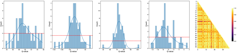
To confirm the validity of uniform and independent assumptions of ensemble Q-learning, we plot Q-value distribution in Figure 1 and test whether each Q-distribution is uniform using the $\chi^{2}$ test. We train 50 Q-networks 3M timesteps by the SAC-Min algorithm in the D4RL hopper-random dataset and evaluate it by the hopper-full-replay dataset. We also perform the $\chi^{2}$ test for independence in Table LABEL:table:num_spike. Out of 1000 batch data, only 35.8% can accept that the distribution is uniform and 30.4% can accept independence. Thus, esโ€‹aiโˆผUโ€‹nโ€‹iโ€‹fโ€‹(โˆ’ฯ„,ฯ„)similar-tosuperscriptsubscript๐‘’๐‘ ๐‘Ž๐‘–๐‘ˆ๐‘›๐‘–๐‘“๐œ๐œe_{sa}^{i}\sim Unif(-\tau,\tau) and i.i.d. assumption is empirically inaccurate and it is necessary to introduce the notion of Q-ensemble independence. More details on the $\chi^{2}$ test are given in Appendix E.

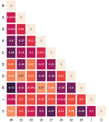
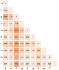
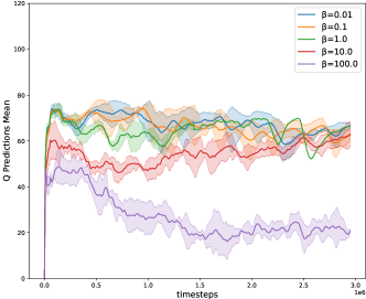
As [30] also points out, the early collapse of Q-values, which means that the Q-values in the ensemble become almost identical, occurs during the training. We empirically visualize a strong correlation among Q-networks in Figure 1. Although the main advantage of ensemble Q-learning is based on diverse Q-functions, network initialization is the only process to maintain diversity over an ensemble since the Bellman target is identical across all networks without diversification and independence regularization methods.

Refer to caption
Figure 2: Eigenvalue plot for the spiked Wishart model with Wignerโ€™s semicircle law. For effective visualization of the spiked model, we use a complex hermitian random matrix, GUE. Blue dots represent each data in a complex plane. The red line represents Wignerโ€™s semicircle distribution. The blue line in the histogram represents kernel density estimation. Left 1โ€“2: Perturbation power is $\psi=0$. Eigenvalue distribution follows Wignerโ€™s semicircle law. Right 3โ€“4: Perturbation power is $\psi=10^{-5}$. Eigenvalue distribution almost follows Wignerโ€™s semicircle law except for the largest eigenvalue, interpreted as a spike.

3.2 Random Matrix Theory

Random matrix theory studies the probabilistic properties of large matrices with random entries. Dyson [10] constructs some categories of the random matrix as a real symmetric matrix as Gaussian orthogonal ensemble (GOE), complex hermitian matrix as Gaussian unitary ensemble (GUE), and quaternion self-dual matrix as Gaussian symplectic ensemble (GSE), called Dysonโ€™s classification. In this paper, we restrict our interest to matrices in GOE.

Definition 3.1 (Gaussian Orthogonal Ensemble, [26]).

Let random matrix $W\in R^{N\times N}$, its entities random variables $w_{i}$, $P[W]=P(w_{1},\dots,w_{N^{2}})$ to be a joint probability density function of $w_{i}$. Define the set of $W$ as GOE when these properties hold:

  1. (1)

    $w_{i}$ are independent with respect to $i$.

  2. (2)

    $W$ is a real symmetric matrix.

  3. (3)

    $W$ is rotational invariance, i.e., $P[W]dW=P[W^{\prime}]dW^{\prime}$ if $W^{\prime}=UWU^{-1}$, $U$ is orthogonal.

GOE is the most natural way to model random matrices in various applications, including machine learning. In simplified terms, we can consider GOE as a Wigner matrix, where entries are independent, symmetric, and follow Gaussian distribution. One of the main areas in random matrix theory is how eigenvalues or singular values of a large random matrix are distributed. More specifically, we only consider limiting properties of empirical spectral density (ESD), which is defined as, for random matrix $W\in\mathbb{R}^{N\times N}$ and its eigenvalues $\lambda_{i},i=1,\dots,N$,

$$\displaystyle p_{W}(\lambda)=\frac{1}{N}\sum\limits_{i=1}^{N}\delta(\lambda-\lambda_{i})$$ (1)

The limits of the empirical spectral density of the GOE, called the Wignerโ€™s semicircle law, are given by [34]. For GOE $\hat{W}\in\mathbb{R}^{N\times N}$ with variance of entries $\sigma^{2}$, $\lambda_{1},\dots,\lambda_{N}$ to be a eigenvalue of $W=\frac{1}{\sqrt{N}}\hat{W}$ and empirical spectral distribution $p_{W}=\frac{1}{N}\sum\limits_{j=1}^{N}\delta(\lambda-\lambda_{j})$, then $p_{W}$ converges to psโ€‹csubscript๐‘๐‘ ๐‘p_{sc} weakly almost surely, where

psโ€‹cโ€‹(ฮป)=12โ€‹ฯ€โ€‹ฯƒ2โ€‹4โ€‹ฯƒ2โˆ’ฮป2โ€‹๐Ÿ™[โˆ’2โ€‹ฯƒ,2โ€‹ฯƒ]subscript๐‘๐‘ ๐‘๐œ†continued-fraction12๐œ‹superscript๐œŽ24superscript๐œŽ2superscript๐œ†2subscript12๐œŽ2๐œŽ\displaystyle p_{sc}(\lambda)=\cfrac{1}{2\pi\sigma^{2}}\sqrt{4\sigma^{2}-\lambda^{2}}\mathbbm{1}_{[-2\sigma,2\sigma]} (2)

We call psโ€‹csubscript๐‘๐‘ ๐‘p_{sc} as the Wignerโ€™s semicircle distribution. Wignerโ€™s semicircle law does not rely on the probability density of entries.

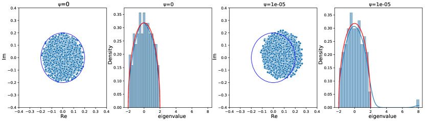
3.3 Spiked Random Model

Random matrix theory models random data well, but in reality, most data have both informative signals and random components. A spiked random model is a theory about constructing a model of perturbation with a data matrix. The objective of this theory is to separate true signals from perturbated ones with random noise. True signals show spiked phenomena that make the largest eigenvalue detach from the bulk of eigenvalues. A spiked model was first introduced by [17] as an application for principal component analysis. We restrict our analysis to a spiked Wishart model, the most natural methodology to model a general perturbation. A spiked Wishart model is defined as follows.

Definition 3.2.

Let $Y\in\mathbb{R}^{N\times M}\sim\mathbb{P}_{\psi}$, $u,v$ is unknown vector, $Y$ is spiked Wishart model when

  1. (1)

    $Y=\sqrt{\frac{\psi}{N}}uv^{T}+W$, which is equivalent to sample covariance matrix $\hat{\Sigma}=I_{N}+\frac{\psi}{N}uu^{T}$

  2. (2)

    $u,v$ are i.i.d from zero mean priors $u\sim P_{u},v\sim P_{v}$, support bounded in radius by $K_{u},K_{v}$

  3. (3)

    $W\sim\mathbb{P}_{0}$ is a matrix with i.i.d noise entries

  4. (4)

    $M/N\rightarrow\omega$

We will assume the spiked Wishart model with $N=M$, where we can ignore property 4. In Figure 2, we visualize how the spiked Wishart model works in both the data and spectral domain. For a detailed explanation, see Appendix A.

4 Q-ensemble Independence Regularization

In this section, we present a method of Q-ensemble independence regularization that is computationally feasible through the utilization of a spiked Wishart model. We bring the concept of ensemble Q-learning to the spiked Wishart model as $Y\sim\mathbb{P}_{\psi}$ representing learned Q-value by Q-learning algorithm and $W\sim\mathbb{P}_{0}$ representing the perfectly independent Q-ensemble. If $W$ dominates $Y$, $Y$ follows independent assumptions of ensemble Q-learning. If not, a collapse of Q-value and high correlation occurs, which cannot be benefited by the ensemble method. By integrating with ensemble Q-learning and Q-ensemble independence testing, we propose a tractable Q-ensemble independence loss with gain $\beta$, which is further described in the following section. To help understand the independence and diversity of Q-ensemble more clearly, we mentioned that $\beta$ can be simply considered as a loss gain (weight) for Q-ensemble independence regularization before providing a detailed explanation about SPQR and $\beta$. A higher $\beta$ represents highly-likely-to-independent.

4.1 Diversity and Independence of Q-ensemble

Refer to caption
Figure 3: Mean of predicted Q-value of SPQR-SAC-Min with various $\beta$ on hopper-random dataset, averaged over 4 seeds.

To clarify our work, we distinguish between the notions of diversity and independence. Numerous ensemble Q-learning methods improve their performance by minimizing the overestimation bias and the variance of the Bellman target estimate. However, such works assume that the biases esโ€‹aisuperscriptsubscript๐‘’๐‘ ๐‘Ž๐‘–e_{sa}^{i} are zero-mean independent and identically distributed over $i$, although early collapse, a high correlation between Q-ensemble, occurs due to the shared Bellman target. On the other hand, diversification methods such as EDAC develop an ensemble diversification objective to reduce the number of ensemble networks required. In particular, EDAC increases the variance of the ensemble to penalize OOD actions. In our work, we focus on the independence of a Q-ensemble to reduce the effect of correlated behavior resulting from a shared Bellman target. Roughly speaking, diversification can be interpreted as flattening the distribution of a Q-ensemble, while independence regularization can be interpreted as promoting an i.i.d. sampling procedure for a given distribution. We verify that our proposed regularization successfully exploits both the conservative behavior and the diversification of a Q-ensemble. The Q-ensemble independence regularization empirically shows a large performance gain by controlling the conservatism, as shown in Figure 3, similar to the performance improvement of the ensemble method caused by the conservatism. For further details, see Appendix E.

4.2 Tractable Loss for Q-ensemble Independence

We construct a tractable testing criterion to determine whether a distribution is independent in Theorem 4.1. DKโ€‹Lโ€‹(pฯˆโ€‹(ฮป),psโ€‹cโ€‹(ฮป))subscript๐ท๐พ๐ฟsubscript๐‘๐œ“๐œ†subscript๐‘๐‘ ๐‘๐œ†D_{KL}(p_{\psi}(\lambda),p_{sc}(\lambda)) does not require any prior assumption about $\mathbb{P}_{0}$ and $\mathbb{P}_{\psi}$ since in spectral domain, Wignerโ€™s semicircle law is universal for all random matrices. Proof of Theorem 4.1 is shown in Appendix B.

Theorem 4.1.

Following definition 3.2, as $N\rightarrow\infty$ with probability at least $1-\delta$, following test $T(\lambda)$ is optimal.

Tโ€‹(ฮป)=๐Ÿ™โ€‹(DKโ€‹Lโ€‹(pฯˆโ€‹(ฮป),psโ€‹cโ€‹(ฮป))โ‰ฅฮต)={H0:Yโˆผโ„™0H1:Yโˆผโ„™ฯˆ๐‘‡๐œ†1subscript๐ท๐พ๐ฟsubscript๐‘๐œ“๐œ†subscript๐‘๐‘ ๐‘๐œ†๐œ€cases:subscript๐ป0similar-to๐‘Œsubscriptโ„™0otherwise:subscript๐ป1similar-to๐‘Œsubscriptโ„™๐œ“otherwise\displaystyle T(\lambda)=\mathbbm{1}(D_{KL}(p_{\psi}(\lambda),p_{sc}(\lambda))\geq\varepsilon)=\begin{cases}H_{0}:Y\sim\mathbb{P}_{0}\\ H_{1}:Y\sim\mathbb{P}_{\psi}\end{cases}

We now describe a practical Q-ensemble independence loss for ensemble Q-learning using the spiked Wishart model and Theorem 4.1. Let $Y$ and $u,v$ for the spiked Wishart model denote a Q-value matrix and an unknown signal. By the test $T(\lambda)$, if DKโ€‹Lโ€‹(pฯˆโ€‹(ฮป),psโ€‹cโ€‹(ฮป))<ฮตsubscript๐ท๐พ๐ฟsubscript๐‘๐œ“๐œ†subscript๐‘๐‘ ๐‘๐œ†๐œ€D_{KL}(p_{\psi}(\lambda),p_{sc}(\lambda))<\varepsilon or is minimized, it is theoretically guaranteed that $Y$ is a random matrix, i.e. a Q-ensemble is independently distributed.

In conclusion, we propose DKโ€‹Lโ€‹(pฯˆโ€‹(ฮป),psโ€‹cโ€‹(ฮป))subscript๐ท๐พ๐ฟsubscript๐‘๐œ“๐œ†subscript๐‘๐‘ ๐‘๐œ†D_{KL}(p_{\psi}(\lambda),p_{sc}(\lambda)) as a Q-ensemble independence regularization loss for ensemble Q-learning, without any prior assumption such as uniform distribution.

4.3 Algorithm

As described in Section 3.1, ensemble Q-learning has crucial but inaccurate assumptions about independence. To address the issue of insufficient independence, we propose SPQR: spiked Wishart Q-ensemble independence regularization for reinforcement learning, which we describe in Algorithm 1. Using the random matrix theory and a spiked random model lens, SPQR minimizes DKโ€‹Lโ€‹(pฯˆโ€‹(ฮป),psโ€‹cโ€‹(ฮป))subscript๐ท๐พ๐ฟsubscript๐‘๐œ“๐œ†subscript๐‘๐‘ ๐‘๐œ†D_{KL}(p_{\psi}(\lambda),p_{sc}(\lambda)) as a form of regularization loss, denoted as SPQR loss, on the baseline ensemble Q-learning algorithms. DKโ€‹Lโ€‹(pฯˆโ€‹(ฮป),psโ€‹cโ€‹(ฮป))subscript๐ท๐พ๐ฟsubscript๐‘๐œ“๐œ†subscript๐‘๐‘ ๐‘๐œ†D_{KL}(p_{\psi}(\lambda),p_{sc}(\lambda)) penalizes for going too far from an independent Q-ensemble, which means promoting Q-ensemble to follow $\mathbb{P}_{0}$. We visualize our concept in Figure 4. To compute the SPQR loss using $p_{\psi}(\lambda)$, we need to construct a symmetric Q-matrix $Y$ filled with Q-values. Then, we normalize the Q-matrix $Y$ with a zero-mean and unit variance to compute the Wignerโ€™s semicircle distribution psโ€‹cโ€‹(ฮป)subscript๐‘๐‘ ๐‘๐œ†p_{sc}(\lambda) with $\sigma=1$. Finally, we compute eigenvalues with a numerically stable algorithm by constructing the ESD $p_{\psi}(\lambda)$ and calculate the KL divergence between $p_{\psi}(\lambda)$ and psโ€‹cโ€‹(ฮป)subscript๐‘๐‘ ๐‘๐œ†p_{sc}(\lambda). The loss function $\mathcal{L}_{SPQR}$ is computed as a expectation of DKโ€‹Lโ€‹(pฯˆโ€‹(ฮป),psโ€‹cโ€‹(ฮป))subscript๐ท๐พ๐ฟsubscript๐‘๐œ“๐œ†subscript๐‘๐‘ ๐‘๐œ†D_{KL}(p_{\psi}(\lambda),p_{sc}(\lambda)) over the batch data. A detailed explanation of implementations and algorithms is shown in Appendix C.

Algorithm 1 SPQR
1:Input: $\gamma,\alpha,N,\beta,\tau,|B|$
2:Initialize policy $\theta$, Q-function $\phi_{i}$, target Q-function $\phi^{\prime}_{i}$, replay buffer $\mathcal{D}$
3:repeat
4:ย ย ย ย ย 

yโ€‹(r,sโ€ฒ)โ†r+ฮณโ€‹(Eโ€‹nโ€‹stโ€‹aโ€‹rโ€‹(ฯ•iโ€ฒ)โˆ’ฮฑโ€‹logโกฯ€ฮธโ€‹(aโ€ฒ|sโ€ฒ))โ†๐‘ฆ๐‘Ÿsuperscript๐‘ โ€ฒ๐‘Ÿ๐›พ๐ธ๐‘›subscript๐‘ ๐‘ก๐‘Ž๐‘Ÿsubscriptsuperscriptitalic-ฯ•โ€ฒ๐‘–๐›ผsubscript๐œ‹๐œƒconditionalsuperscript๐‘Žโ€ฒsuperscript๐‘ โ€ฒy(r,s^{\prime})\leftarrow r+\gamma\biggl{(}\color[rgb]{0,0,1}\definecolor[named]{pgfstrokecolor}{rgb}{0,0,1}Ens_{tar}(\phi^{\prime}_{i})\color[rgb]{0,0,0}\definecolor[named]{pgfstrokecolor}{rgb}{0,0,0}\pgfsys@color@gray@stroke{0}\pgfsys@color@gray@fill{0}-\alpha\log\pi_{\theta}(a^{\prime}|s^{\prime})\biggr{)}

5:ย ย ย ย ย forย i=1,โ€ฆ,N๐‘–1โ€ฆ๐‘i=1,\dots,Nย do
6:ย ย ย ย ย ย ย ย ย 

โ„’Sโ€‹Pโ€‹Qโ€‹R=DKโ€‹Lโ€‹(pฯˆโ€‹(ฮป),psโ€‹cโ€‹(ฮป))subscriptโ„’๐‘†๐‘ƒ๐‘„๐‘…subscript๐ท๐พ๐ฟsubscript๐‘๐œ“๐œ†subscript๐‘๐‘ ๐‘๐œ†\mathcal{L}_{SPQR}=D_{KL}(p_{\psi}(\lambda),p_{sc}(\lambda))

7:ย ย ย ย ย ย ย ย ย 

โˆ‡ฯ•i1|B|โ€‹โˆ‘(Qฯ•iโ€‹(s,a)โˆ’yโ€‹(r,sโ€ฒ))2+ฮฒโ€‹โ„’Sโ€‹Pโ€‹Qโ€‹Rsubscriptโˆ‡subscriptitalic-ฯ•๐‘–continued-fraction1๐ตsuperscriptsubscript๐‘„subscriptitalic-ฯ•๐‘–๐‘ ๐‘Ž๐‘ฆ๐‘Ÿsuperscript๐‘ โ€ฒ2๐›ฝsubscriptโ„’๐‘†๐‘ƒ๐‘„๐‘…\nabla_{\phi_{i}}\cfrac{1}{|B|}\sum(Q_{\phi_{i}}(s,a)-y(r,s^{\prime}))^{2}\color[rgb]{0,0,1}\definecolor[named]{pgfstrokecolor}{rgb}{0,0,1}+\beta\mathcal{L}_{SPQR}

8:ย ย ย ย ย endย for
9:ย ย ย ย ย 

โˆ‡ฮธ1|B|โ€‹โˆ‘sโˆˆB(Eโ€‹nโ€‹seโ€‹vโ€‹aโ€‹lโ€‹(ฯ•i)โˆ’ฮฑโ€‹logโกฯ€ฮธโ€‹(a~|s))subscriptโˆ‡๐œƒcontinued-fraction1๐ตsubscript๐‘ ๐ต๐ธ๐‘›subscript๐‘ ๐‘’๐‘ฃ๐‘Ž๐‘™subscriptitalic-ฯ•๐‘–๐›ผsubscript๐œ‹๐œƒconditional~๐‘Ž๐‘ \nabla_{\theta}\cfrac{1}{|B|}\sum_{s\in B}\biggl{(}\color[rgb]{0,0,1}\definecolor[named]{pgfstrokecolor}{rgb}{0,0,1}Ens_{eval}(\phi_{i})\color[rgb]{0,0,0}\definecolor[named]{pgfstrokecolor}{rgb}{0,0,0}\pgfsys@color@gray@stroke{0}\pgfsys@color@gray@fill{0}-\alpha\log\pi_{\theta}(\tilde{a}|s)\biggr{)}

10:untilย 

Algorithm 2 SPQR Loss
1:Input: Q-network lk={Qฯ•iโ€‹(sโ€ฒ,aโ€ฒ)}i=1Nsubscript๐‘™๐‘˜superscriptsubscriptsubscript๐‘„subscriptitalic-ฯ•๐‘–superscript๐‘ โ€ฒsuperscript๐‘Žโ€ฒ๐‘–1๐‘l_{k}=\{Q_{\phi_{i}}(s^{\prime},a^{\prime})\}_{i=1}^{N}
2:$Y\in\mathbb{R}^{D\times D},\,D=\lfloor\frac{\sqrt{1+8N}-1}{2}\rfloor$:
3:$Y_{pq}\leftarrow\begin{cases}l_{Dp+q},&\text{if}\;p\geq q\\ Y_{qp},&\text{otherwise}\end{cases}$
4:$Y\leftarrow(Y-\mu_{Y})/\sigma_{Y}$
5:$\{\lambda_{i}\}_{i=1}^{N}\leftarrow Eigen(\frac{1}{\sqrt{N}}Y)$
6:peโ€‹sโ€‹dโ€‹(ฮป)=1Nโ€‹โˆ‘iฮดโ€‹(ฮปโˆ’ฮปi)subscript๐‘๐‘’๐‘ ๐‘‘๐œ†1๐‘subscript๐‘–๐›ฟ๐œ†subscript๐œ†๐‘–p_{esd}(\lambda)=\frac{1}{N}\sum_{i}\delta(\lambda-\lambda_{i})
7:$p_{wigner}(\lambda)=\frac{\sqrt{4-\lambda^{2}}}{2\pi}$
8:

โ„’Sโ€‹Pโ€‹Qโ€‹Rโ†1|B|โ€‹โˆ‘jโˆ‘ipeโ€‹sโ€‹dโ€‹(ฮปi)โ€‹logโกpeโ€‹sโ€‹dโ€‹(ฮปi)pwโ€‹iโ€‹gโ€‹nโ€‹eโ€‹rโ€‹(ฮปi)โ†subscriptโ„’๐‘†๐‘ƒ๐‘„๐‘…1๐ตsubscript๐‘—subscript๐‘–subscript๐‘๐‘’๐‘ ๐‘‘subscript๐œ†๐‘–continued-fractionsubscript๐‘๐‘’๐‘ ๐‘‘subscript๐œ†๐‘–subscript๐‘๐‘ค๐‘–๐‘”๐‘›๐‘’๐‘Ÿsubscript๐œ†๐‘–\mathcal{L}_{SPQR}\leftarrow\frac{1}{|B|}\sum_{j}\sum_{i}p_{esd}(\lambda_{i})\log{\cfrac{p_{esd}(\lambda_{i})}{p_{wigner}(\lambda_{i})}}

9:Output: SPQR loss $\mathcal{L}_{SPQR}$
[Uncaptioned image]
Figure 4: Illustrative example of SPQR.
[Uncaptioned image]
Figure 5: Illustration for building Q-matrix.

5 Experimental Results

To reveal the validity and universality of SPQR from algorithms to tasks, we implement SPQR in various ensemble Q-learning algorithms and various online/offline RL tasks. We implement SPQR in SAC-Ens, REDQ, SAC-Min, and CQL, and evaluate them in online MuJoCo Gym tasks, offline D4RL Gym, Franka Kitchen, and Antmaze tasks. We denote the SPQR-implemented version of each ensemble algorithm as SPQR-$*$, such as SPQR-SAC-Ens. All the following implementations use the same hyperparameter and experimental protocol with a baseline. For fair evaluation, the SPQR code is written on top of each official baseline code, REDQ111https://github.com/watchernyu/REDQ, EDAC222https://github.com/snu-mllab/EDAC, and CQL333 https://github.com/aviralkumar2907/CQL. Implementation of SPQR can be done by only 50 lines and training time only increases by 5%. We empirically show that SPQR outperforms baseline ensemble Q-learning algorithms in both online and offline RL tasks. See the implementation details in Appendix D.

Is SPQR really affecting independence?

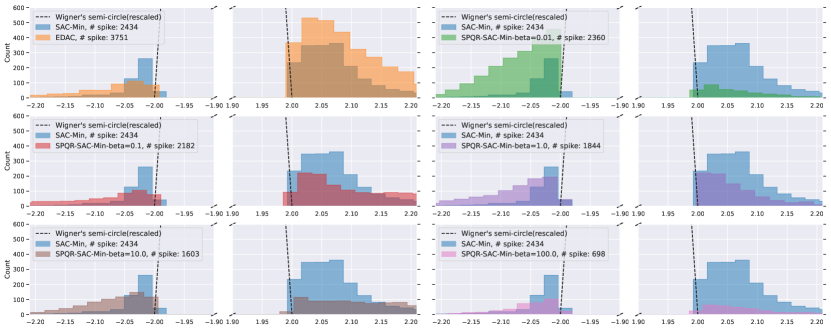
We perform independence hypothesis testing and visualize the spectral distribution to investigate whether SPQR really affects the independence of the Q-ensemble. First, we analyze the performance gain of SPQR from a spike reduction perspective. We train a Q-ensemble using SAC-Min and SPQR-SAC-Min on the hopper-random dataset and test it on the hopper-full-replay dataset. Figure 6 and Table LABEL:table:num_spike show the evaluation results for the spike-reducing phenomenon of SPQR, which deviates less from Wignerโ€™s semicircle law. Compared to SPQR-SAC-Min with $\beta=0.1$, SAC-Min has significantly more spikes, in particular, 2434 spikes compared to 2182 spikes over 25600 data. For extreme regularization gain, $\beta=100$, the spike is drastically reduced to 698, 71% less than the baseline algorithm. We also plot a spike histogram for another diversification method, EDAC. EDAC increases spikes to 54% more than SAC-Min, which can be interpreted as SPQR being the orthogonal method with EDAC.

We also demonstrate the $\chi^{2}$ test with null hypothesis $H_{0}:P(Q_{i},Q_{j})=P(Q_{i})P(Q_{j})$ and significant level $\alpha=0.025$ for independence hypothesis testing on the same experimental setting above. Since SPQR promotes being "more" independent, we use the proportion of data that can accept an independent hypothesis as a measure of more or less independence. In Table LABEL:table:num_spike, we report the proportion of trials over 1000 tests that accept the null hypothesis $H_{0}$, meaning that the Q-ensemble is independent. These empirical studies can be interpreted as SPQR having Q-ensemble independence regularization power since the acceptance rate increases monotonically as $\beta$ increases. Orthogonality between SPQR and EDAC is also found from an independence testing perspective. However, reducing spikes and being more independent does not guarantee optimal performance since there is an optimal conservatism for each task. We can find the proper conservatism by controlling the independence regularization power, $\beta$. More details can be found in Appendix E.

[Uncaptioned image]
Figure 6: Histogram of spikes for Wignerโ€™s semicircle (black line), SAC-Min (blue), EDAC (orange), and SPQR-$\beta=100.0$ (green). For effective visualization, we plot only the eigenvalues that violate Wignerโ€™s semicircle.
Table 1: Number of spikes, independence hypothesis testing acceptance ratio, and performance of SAC-Min, EDAC, and SPQR-$\beta=0.01,0.1,1.0,10.0,100.0$. We reproduce EDAC-$\eta=1.0$. The reported value of EDAC-$\eta=1.0$ is given in the Section H of [2]
Algorithm Spike Performance Accept ratio
SAC-Min 2434 $31.3\pm 0.0$ 30.4%
EDAC-$\eta=1.0$ 3751 $10.3\pm 0.2$ 0.0%
SPQR-$\beta=0.01$ 2360 $33.6\pm 1.8$ 59.0%
SPQR-$\beta=0.1$ 2182 $\textbf{35.6}\pm\textbf{1.4}$ 80.4%
SPQR-$\beta=1.0$ 1844 $32.6\pm 0.4$ 91.4%
SPQR-$\beta=10.0$ 1603 $32.7\pm 0.4$ 92.3%
SPQR-$\beta=100.0$ 698 $32.9\pm 0.8$ 97.6%
Refer to caption
Figure 7: Average returns of SPQR-SAC-Ens, SPQR-REDQ-UTD=1, and SPQR-REDQ-UTD=20 on the MuJoCo environment. Averaged over 4 random seeds.
Table 2: Normalized average returns of SPQR-SAC-Min and SPQR-CQL-Min on D4RL Gym, Franka Kitchen, and Antmaze tasks, averaged over 4 random seeds. Except for SPQR-$*$, the evaluated values of baselines are reported refer to [2, 21], and reproduced for $*$-full-replay tasks of CQL-Min. Reproduced values are indicated as italic font.
Gym BC CQL-Min EDAC SAC-Min SPQR-SAC-Min
walker2d-random $1.3\pm 0.1$ 7.0 $16.6\pm 7.0$ $21.7\pm 0.0$ $\textbf{24.6}\pm\textbf{1.1}$
walker2d-medium $70.9\pm 11.0$ 74.5 $92.5\pm 0.8$ $87.9\pm 0.2$ $\textbf{98.4}\pm\textbf{2.0}$
walker2d-expert $108.7\pm 0.2$ 121.6 $115.1\pm 1.9$ $116.7\pm 0.4$ $115.2\pm 1.3$
walker2d-medium-expert $90.1\pm 13.2$ 98.7 $114.7\pm 0.9$ $116.7\pm 0.4$ $\textbf{118.2}\pm\textbf{0.7}$
walker2d-medium-replay $20.3\pm 9.8$ 32.6 $87.1\pm 2.3$ $78.7\pm 0.7$ $\textbf{87.8}\pm\textbf{2.5}$
walker2d-full-replay $68.8\pm 17.7$ 98.96 $99.8\pm 0.7$ $94.6\pm 0.5$ $\textbf{101.1}\pm\textbf{0.4}$
halfcheetah-random $2.2\pm 0.0$ 35.4 $28.4\pm 1.0$ $28.0\pm 0.9$ $33.5\pm 2.5$
halfcheetah-medium $43.2\pm 0.6$ 44.4 $65.9\pm 0.6$ $67.5\pm 1.2$ $\textbf{74.8}\pm\textbf{1.3}$
halfcheetah-expert $91.8\pm 1.5$ 104.8 $106.8\pm 3.4$ $105.2\pm 2.6$ $\textbf{112.8}\pm\textbf{0.3}$
halfcheetah-medium-expert $44.0\pm 1.6$ 62.4 $106.3\pm 1.9$ $107.1\pm 2.0$ $\textbf{114.0}\pm\textbf{1.6}$
halfcheetah-medium-replay $37.6\pm 2.1$ 46.2 $61.3\pm 1.9$ $63.9\pm 0.8$ $\textbf{69.7}\pm\textbf{1.4}$
halfcheetah-full-replay $62.9\pm 0.8$ 82.07 $84.6\pm 0.9$ $84.5\pm 1.2$ $\textbf{88.5}\pm\textbf{0.5}$
hopper-random $3.7\pm 0.6$ 7.0 $25.3\pm 10.4$ $31.3\pm 0.0$ $\textbf{35.6}\pm\textbf{1.4}$
hopper-medium $54.1\pm 3.8$ 86.6 $\textbf{101.6}\pm\textbf{0.6}$ $100.3\pm 0.3$ $100.2\pm 1.3$
hopper-expert $107.7\pm 9.7$ 109.9 $110.1\pm 0.1$ $110.3\pm 0.3$ $\textbf{112.0}\pm\textbf{0.2}$
hopper-medium-expert $53.9\pm 4.7$ 111.0 $110.7\pm 0.1$ $110.1\pm 0.3$ $\textbf{112.5}\pm\textbf{0.3}$
hopper-medium-replay $16.6\pm 4.8$ 48.6 $101.0\pm 0.5$ $101.8\pm 0.5$ $\textbf{104.9}\pm\textbf{0.7}$
hopper-full-replay $19.9\pm 12.9$ 104.85 $105.4\pm 0.7$ $102.9\pm 0.3$ $\textbf{109.1}\pm\textbf{0.4}$
Average 49.9 70.9 85.2 84.5 89.6
Franka Kitchen BC SAC-Min BEAR CQL-Min SPQR-CQL-Min
kitchen-complete $33.8$ $15.0$ $0.0$ $43.8$ $\textbf{47.9}\pm\textbf{12.3}$
kitchen-partial $33.8$ $0.0$ $13.1$ $49.8$ $\textbf{54.2}\pm\textbf{7.2}$
kitchen-mixed $47.5$ $2.5$ $47.2$ $51.0$ $\textbf{55.6}\pm\textbf{7.9}$
Average 38.4 5.8 20.1 48.2 52.6
Antmaze BC SAC-Min BEAR CQL-Min SPQR-CQL-Min
umaze 65.0 0.0 73.0 74.0 $\textbf{93.3}\pm\textbf{4.7}$
umaze-diverse 55.0 0.0 61.0 84.0 $80.0\pm 0.0$
medium-play 0.0 0.0 0.0 61.2 $\textbf{80.0}\pm\textbf{8.2}$
Average 40.0 0.0 44.7 73.1 84.4

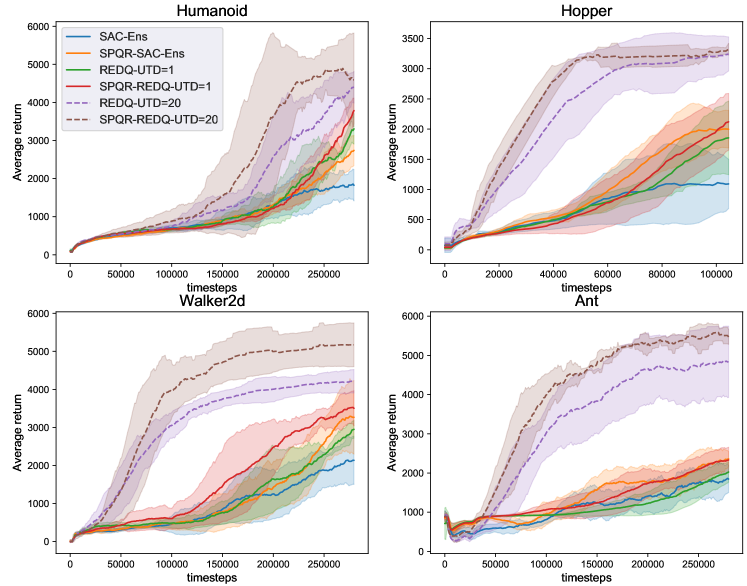
Online Reinforcement Learning.

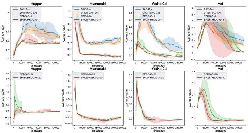
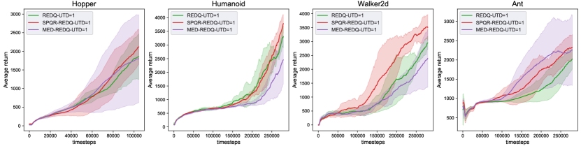
We implement SPQR-SAC-Ens and SPQR-REDQ with UTD ratio 1 and 20, and compare them to SAC-Ens and REDQ to show how SPQR improves performance. We evaluate each algorithm on the OpenAI Gym MuJoCo tasks. Figure 7 shows the training curves for SAC-Ens, REDQ, SPQR-SAC-Ens, and SPQR-REDQ. Since the two main contributions of REDQ, UTD ratio, and subset minimization, are orthogonal methods to each other, we experiment with SPQR-REDQ for UTD ratio 1 and 20. A high UTD ratio can be interpreted as frequent gradient updates, thereby resulting in better performance. For each algorithm, we plot the average return as a solid curve and the standard deviation as a shaded area. The implementation of SPQR yields notable improvements in the performance of SAC-Ens and REDQ across all tasks, as well as under both UTD ratio 1 and 20 conditions. Specifically, SPQR-SAC-Ens performs 2 times better than SAC-Ens on the Hopper task. Also, SPQR-REDQ-UTD=1 and SPQR-REDQ-UTD=20 show 1.1 and 1.3 times better than REDQ-UTD=1 and REDQ-UTD=20 for the Walker2d and Ant tasks.

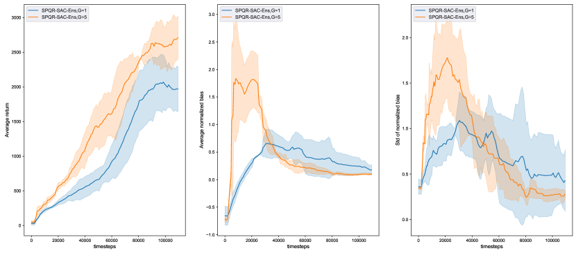
To investigate why SPQR performs better, we evaluate the bias of the Q-value computed by the Monte-Carlo algorithm. The average of the Q-bias decreases with SPQR, which can be interpreted as the relationship between the distribution of the ensemble becoming more independent. We also evaluate the ablation study for the UTD ratio. SPQR-SAC-Ens shows performance improvement and bias alleviation with low standard deviation as the UTD ratio increases although high UTD SAC causes large and unstable bias. In terms of diversity, we also evaluate the standard deviation with different $\beta$ for SPQR. As $\beta$ increases, the standard deviation for explored state-action also increases in all training timesteps. In summary, Q-ensemble independence is the key factor in improving the performance of SPQR. Further details and experimental results can be found in Appendix E.

Offline Reinforcement Learning.

SAC-Min is formally constructed and evaluated in [2]. We follow the reported value and evaluation protocol from the paper. We consider baseline behavior cloning (BC), CQL, EDAC, and SAC-Min. The evaluation results of SPQR-SAC-Min compared with SAC-Min and other baselines are shown in Table LABEL:table:offline_d4rl_result. For most tasks, SPQR outperforms all baselines well. Specifically, for $*$-random dataset, SPQR improves SAC-Min by about 16% when CQL and EDAC fail for $*$-random dataset. It implies that SPQR is robust for the quality of data. Since SPQR gives more conservatism, which shows identical behavior with increasing ensemble size $N$, SPQR-SAC-Min needs a smaller number of ensemble networks to outperform SAC-Min. For the hopper-medium, SAC-Min uses 500 Q-networks and SPQR uses only 50 Q-networks, which is about 90% efficient in terms of computational cost. It implies that the independence regularization of the Q-ensemble becomes computationally efficient.

We also implement SPQR to CQL($\mathcal{H}$), denoted as SPQR-CQL-Min. Referring to the implementation details in the paper and the original baseline code of CQL, the original CQL uses a twin Q-function trick, which is equivalent to SAC-Min with $N=2$. We modified CQL as CQL-Min to use $N$ Q-networks to compute the Bellman target. Hence, the original CQL can be called CQL-Min with $N=2$. We evaluate SPQR-CQL-Min on D4RL Franka Kitchen and Antmaze, one of the most complex and sparse tasks in D4RL.

In Table LABEL:table:offline_d4rl_result, we evaluate SPQR-CQL-Min with other baseline methods. SPQR-CQL-Min outperforms all baseline algorithms, notably 2.6 times better than BEAR. For Franka Kitchen tasks, SPQR consistently improves CQL by 10% for all three tasks, which can be interpreted as robustness over the quality of data. Surprisingly, SPQR achieves the maximum score on 3 different Antmaze tasks, which outperforms all existing algorithms. Further details and results are presented in Appendix D and E.

Can other diversification methods benefit from the SPQR?

Since SPQR regularizes Q-ensemble independence, which is the orthogonal method with other diversification methods, we implement SPQR in EDAC to benefit from the combination of two orthogonal methods. We evaluate SPQR-EDAC for the tasks where EDAC outperforms the baseline algorithm SAC-Min. SPQR and SPQR-EDAC show large performance gains over SAC-Min, as shown in Table LABEL:table:spqr_edac.

Table 3: Normalized average returns of SPQR-SAC-Min and SPQR-EDAC on D4RL Gym tasks, averaged over 4 random seeds. Except for SPQR-$*$, the evaluated values of baselines are reported. Refer to [2].
Gym EDAC SAC-Min SPQR-SAC-Min SPQR-EDAC
walker2d-medium $92.5\pm 0.8$ $87.9\pm 0.2$ $\textbf{98.4}\pm\textbf{2.0}$ $94.8\pm 1.0$
walker2d-medium-replay $87.1\pm 2.3$ $78.7\pm 0.7$ $87.8\pm 2.5$ $\textbf{89.6}\pm\textbf{1.8}$
walker2d-full-replay $99.8\pm 0.7$ $94.6\pm 0.5$ $101.1\pm 0.4$ $\textbf{102.2}\pm\textbf{0.2}$
halfcheetah-expert $106.8\pm 3.4$ $105.2\pm 2.6$ $\textbf{112.8}\pm\textbf{0.3}$ $110.3\pm 0.2$
halfcheetah-full-replay $84.6\pm 0.9$ $84.5\pm 1.2$ $\textbf{88.5}\pm\textbf{0.5}$ $86.8\pm 0.2$
hopper-medium $101.6\pm 0.6$ $100.3\pm 0.3$ $100.2\pm 1.3$ $\textbf{103.8}\pm\textbf{0.1}$
hopper-medium-expert $110.7\pm 0.1$ $110.1\pm 0.3$ $\textbf{112.5}\pm\textbf{0.3}$ $111.7\pm 0.0$
hopper-full-replay $105.4\pm 0.7$ $102.9\pm 0.3$ $\textbf{109.1}\pm\textbf{0.4}$ $108.2\pm 0.5$

6 Conclusions

We propose SPQR, a Q-ensemble independence regularization framework for ensemble Q-learning by applying random matrix theory and a spiked random model. We theoretically propose a tractable loss for Q-ensemble independence. The proposed theoretical approach does not require any prior assumption on the Q-function distribution, such as uniform distribution or i.i.d. In addition, we present the difference between diversity and independence and empirically show the orthogonality of the diversification method and SPQR. Furthermore, SPQR serves as a conservatism control framework for ensemble Q-learning by effectively regularizing independence with various empirical evidence. We also empirically show that SPQR is computationally efficient and outperforms many existing ensemble Q-learning algorithms on various online and offline RL benchmark tasks.

Acknowledgements

We appreciate Minyoung Kim for creating an illustration for our paper, as well as Jaehoon Choi and Yejin Kim for writing advice. We also thank the anonymous reviewers for their insightful feedback and reviews. This work is in part supported by National Research Foundation of Korea (NRF, 2021R1A2C2014504(20%), 2021M3F3A2A02037893(20%)), Institute of Information & communications Technology Planning & Evaluation (IITP, 2021-0-00106(20%), 2021-0-01059(20%), 2021-0-02068(20%)) grant funded by the Ministry of Science and ICT (MSIT), INMAC and BK21 FOUR Program.

References

  • Ahn etย al. [2022] Michael Ahn, Anthony Brohan, Noah Brown, Yevgen Chebotar, Omar Cortes, Byron David, Chelsea Finn, Chuyuan Fu, Keerthana Gopalakrishnan, Karol Hausman, Alex Herzog, Daniel Ho, Jasmine Hsu, Julian Ibarz, Brian Ichter, Alex Irpan, Eric Jang, Rosarioย Jauregui Ruano, Kyle Jeffrey, Sally Jesmonth, Nikhilย J Joshi, Ryan Julian, Dmitry Kalashnikov, Yuheng Kuang, Kuang-Huei Lee, Sergey Levine, Yao Lu, Linda Luu, Carolina Parada, Peter Pastor, Jornell Quiambao, Kanishka Rao, Jarek Rettinghouse, Diego Reyes, Pierre Sermanet, Nicolas Sievers, Clayton Tan, Alexander Toshev, Vincent Vanhoucke, Fei Xia, Ted Xiao, Peng Xu, Sichun Xu, Mengyuan Yan, and Andy Zeng. Do as i can, not as i say: Grounding language in robotic affordances, 2022.
  • An etย al. [2021] Gaon An, Seungyong Moon, Jang-Hyun Kim, and Hyunย Oh Song. Uncertainty-based offline reinforcement learning with diversified q-ensemble. In NeurIPS, pages 7436โ€“7447, 2021.
  • Anschel etย al. [2017] Oron Anschel, Nir Baram, and Nahum Shimkin. Averaged-dqn: Variance reduction and stabilization for deep reinforcement learning. In International conference on machine learning, pages 176โ€“185. PMLR, 2017.
  • Banks etย al. [2018] Jess Banks, Cristopher Moore, Roman Vershynin, Nicolas Verzelen, and Jiaming Xu. Information-theoretic bounds and phase transitions in clustering, sparse pca, and submatrix localization. IEEE Transactions on Information Theory, 64(7):4872โ€“4894, 2018.
  • Baskerville etย al. [2022] Nicholasย P Baskerville, Diego Granziol, and Jonathanย P Keating. Appearance of random matrix theory in deep learning. Physica A: Statistical Mechanics and its Applications, 590:126742, 2022.
  • Chen etย al. [2021] Xinyue Chen, Che Wang, Zijian Zhou, and Keithย W. Ross. Randomized ensembled double q-learning: Learning fast without a model. In International Conference on Learning Representations, 2021.
  • Chung and Lee [2019] Hyeย Won Chung and Jiย Oon Lee. Weak detection of signal in the spiked wigner model. In Kamalika Chaudhuri and Ruslan Salakhutdinov, editors, Proceedings of the 36th International Conference on Machine Learning, volumeย 97 of Proceedings of Machine Learning Research, pages 1233โ€“1241. PMLR, 09โ€“15 Jun 2019.
  • Cocola etย al. [2020] Jorio Cocola, Paul Hand, and Vlad Voroninski. Nonasymptotic guarantees for spiked matrix recovery with generative priors. Advances in Neural Information Processing Systems, 33:15185โ€“15197, 2020.
  • [9] Momar Dieng. On the distribution of eigenvalues and their spacings: a rapid introduction to random matrix theory.
  • Dyson [1962] Freemanย J Dyson. The threefold way. algebraic structure of symmetry groups and ensembles in quantum mechanics. Journal of Mathematical Physics, 3(6):1199โ€“1215, 1962.
  • Elย Abidi [2018] Ahmed Elย Alaoui Elย Abidi. Detection limits and fluctuation results in some spiked random matrix models and pooling of discrete data. University of California, Berkeley, 2018.
  • FAIR etย al. [2022] FAIR, Anton Bakhtin, Noam Brown, Emily Dinan, Gabriele Farina, Colin Flaherty, Daniel Fried, Andrew Goff, Jonathan Gray, Hengyuan Hu, Athulย Paul Jacob, Mojtaba Komeili, Karthik Konath, Minae Kwon, Adam Lerer, Mike Lewis, Alexanderย H. Miller, Sasha Mitts, Adithya Renduchintala, Stephen Roller, Dirk Rowe, Weiyan Shi, Joe Spisak, Alexander Wei, David Wu, Hugh Zhang, and Markus Zijlstra. Human-level play in the game of diplomacy by combining language models with strategic reasoning. Science, 378(6624):1067โ€“1074, 2022.
  • Fu etย al. [2020] Justin Fu, Aviral Kumar, Ofir Nachum, George Tucker, and Sergey Levine. D4rl: Datasets for deep data-driven reinforcement learning. arXiv preprint arXiv:2004.07219, 2020.
  • Giles [2008] Mike Giles. An extended collection of matrix derivative results for forward and reverse mode automatic differentiation. 2008.
  • Hasselt [2010] Hado Hasselt. Double q-learning. Advances in neural information processing systems, 23, 2010.
  • Ionescu etย al. [2015] Catalin Ionescu, Orestis Vantzos, and Cristian Sminchisescu. Matrix backpropagation for deep networks with structured layers. In 2015 IEEE International Conference on Computer Vision (ICCV), pages 2965โ€“2973, 2015. doi: 10.1109/ICCV.2015.339.
  • Johnstone [2001] Iainย M Johnstone. On the distribution of the largest eigenvalue in principal components analysis. The Annals of statistics, 29(2):295โ€“327, 2001.
  • Jung etย al. [2021] Jiย Hyung Jung, Hyeย Won Chung, and Jiย Oon Lee. Detection of signal in the spiked rectangular models. In Marina Meila and Tong Zhang, editors, Proceedings of the 38th International Conference on Machine Learning, volume 139 of Proceedings of Machine Learning Research, pages 5158โ€“5167. PMLR, 18โ€“24 Jul 2021.
  • Keener [2010] Robertย W Keener. Theoretical statistics: Topics for a core course. Springer, 2010.
  • Kostrikov etย al. [2021] Ilya Kostrikov, Ashvin Nair, and Sergey Levine. Offline reinforcement learning with implicit q-learning. CoRR, abs/2110.06169, 2021. URL https://arxiv.org/abs/2110.06169.
  • Kumar etย al. [2020] Aviral Kumar, Aurick Zhou, George Tucker, and Sergey Levine. Conservative q-learning for offline reinforcement learning. Advances in Neural Information Processing Systems, 33:1179โ€“1191, 2020.
  • Lan etย al. [2020] Qingfeng Lan, Yangchen Pan, Alona Fyshe, and Martha White. Maxmin q-learning: Controlling the estimation bias of q-learning. In International Conference on Learning Representations, 2020.
  • LeCam [1960] Lucien LeCam. Locally asymptotically normal families of distributions. Univ. California Publ. Statist., 3:37โ€“98, 1960.
  • Lee etย al. [2021] Kimin Lee, Michael Laskin, Aravind Srinivas, and Pieter Abbeel. Sunrise: A simple unified framework for ensemble learning in deep reinforcement learning. In Marina Meila and Tong Zhang, editors, Proceedings of the 38th International Conference on Machine Learning, volume 139 of Proceedings of Machine Learning Research, pages 6131โ€“6141. PMLR, 18โ€“24 Jul 2021.
  • Liao and Couillet [2018] Zhenyu Liao and Romain Couillet. The dynamics of learning: A random matrix approach. In International Conference on Machine Learning, pages 3072โ€“3081. PMLR, 2018.
  • Mehta [1967] M.L. Mehta. Random matrices and the statistical theory of energy levels, 1967.
  • Pearson [1900] Karl Pearson. X. on the criterion that a given system of deviations from the probable in the case of a correlated system of variables is such that it can be reasonably supposed to have arisen from random sampling. The London, Edinburgh, and Dublin Philosophical Magazine and Journal of Science, 50(302):157โ€“175, 1900.
  • Schrittwieser etย al. [2019] Julian Schrittwieser, Ioannis Antonoglou, Thomas Hubert, Karen Simonyan, Laurent Sifre, Simon Schmitt, Arthur Guez, Edward Lockhart, Demis Hassabis, Thore Graepel, Timothyย P. Lillicrap, and David Silver. Mastering atari, go, chess and shogi by planning with a learned model. CoRR, abs/1911.08265, 2019.
  • Seddik etย al. [2020] Mohamed Elย Amine Seddik, Cosme Louart, Mohamed Tamaazousti, and Romain Couillet. Random matrix theory proves that deep learning representations of gan-data behave as gaussian mixtures. In International Conference on Machine Learning, pages 8573โ€“8582. PMLR, 2020.
  • Sheikh etย al. [2022a] Hassam Sheikh, Kizza Frisbee, and Mariano Phielipp. DNS: Determinantal point process based neural network sampler for ensemble reinforcement learning. In Kamalika Chaudhuri, Stefanie Jegelka, Leย Song, Csaba Szepesvari, Gang Niu, and Sivan Sabato, editors, Proceedings of the 39th International Conference on Machine Learning, volume 162 of Proceedings of Machine Learning Research, pages 19731โ€“19746. PMLR, 17โ€“23 Jul 2022a.
  • Sheikh etย al. [2022b] Hassam Sheikh, Mariano Phielipp, and Ladislau Boloni. Maximizing ensemble diversity in deep reinforcement learning. In International Conference on Learning Representations, 2022b.
  • Vanย der Maaten and Hinton [2008] Laurens Vanย der Maaten and Geoffrey Hinton. Visualizing data using t-sne. Journal of machine learning research, 9(11), 2008.
  • Vanย der Vaart [2000] Aadย W Vanย der Vaart. Asymptotic statistics, volumeย 3. Cambridge university press, 2000.
  • Wigner [1955] Eugeneย P. Wigner. Characteristic vectors of bordered matrices with infinite dimensions. Annals of Mathematics, 62(3):548โ€“564, 1955. ISSN 0003486X.

Appendix A Review for Detection Theory and Spiked Random Model

We call strong detection when we perfectly detect the presence of a spike signal and weak detection when we detect the presence of a spike signal with some error by hypothesis testing. A formal definition for a strong detection can be constructed under the notion of contiguity by [23]. The contiguity of the spiked Wishart model is proven by the second moment method, which means that we cannot distinguish without error whether data is pure noise or contains some signal.

Definition A.1 (Contiguity).

Let $P_{n}$ and $Q_{n}$ be two sequences of probability measures defined on the sequence of measurable spaces $(\Omega_{n},\mathcal{F}_{n})$. $Q_{n}$ is contiguous with respect to the sequence $P_{n}$ if $P_{n}(A_{n})\rightarrow 0$ implies $Q_{n}(A_{n})\rightarrow 0$ as $n\rightarrow\infty$ for every sequence of measurable sets $A_{n}\in\mathcal{F}_{n}$, denoted as $Q_{n}\lhd P_{n}$. The sequences $P_{n}$ and $Q_{n}$ are mutually contiguous if both $Q_{n}\lhd P_{n}$ and $P_{n}\lhd Q_{n}$ holds, denoted as $Q_{n}\lhd\rhd P_{n}$

Lemma A.2 (Le Camโ€™s First Lemma).

Let $P_{n}$ and $Q_{n}$ be two sequences of probability measures defined on the sequence of measurable spaces $(\Omega_{n},\mathcal{F}_{n})$. Then the following statements are equivalent:
1. $Q_{n}\lhd P_{n}$
2. If $dP_{n}/dQ_{n}\xrightarrow{Q_{n}}U$ along a subsequence, then $P(U>0)=1$
3. If $dQ_{n}/dP_{n}\xrightarrow{P_{n}}V$ along a subsequence, then $\mathbb{E}[V]=1$
4. For any statistics $T_{n}:\Omega_{n}\mapsto\mathbb{R}^{k}$, If $T_{n}\xrightarrow{P_{n}}0$, then $T_{n}\xrightarrow{Q_{n}}0$

Lemma A.3 (Second moment method).

Let $P_{n}$ and $Q_{n}$ be two sequences of probability measures defined on the sequence of measurable spaces $(\Omega_{n},\mathcal{F}_{n})$, and Radon-Nikodym derivative of $P_{n}$ with respect to $Q_{n}$ as $L_{n}\equiv dP_{n}/dQ_{n}$. If $\limsup\mathbb{E}_{Q_{n}}[L_{n}^{2}]<\infty$, then $P_{n}\lhd Q_{n}$

Lemma A.4.

For spiked wishart model following definition 3.2, $K_{u}^{4}K_{v}^{4}\psi^{2}<1$, the families of distributions $\mathbb{P}_{0}$ and $\mathbb{P}_{\psi}$,indexed by $M,N$, are mutually contiguous in the limit $N\rightarrow\infty,M/N\rightarrow\omega$

Hypothesis Testing for Weak Detection.

To distinguish whether spiked Wishart model $Y$ follows $\mathbb{P}_{\psi}$ or $\mathbb{P}_{0}$, detection error is inevitable since contiguity holds. Even if the perfect test is not available, it needs to be better than a random guess, which is achievable by constructing a hypothesis test. Let $(\Omega,\mathcal{F},\hat{\rho})$ be a probability space, $(\mathcal{X},\mathcal{B})$ be a topological space with Borel $\sigma$-algebra $\mathcal{B}$, and $\Theta$ to be a set of parameters. For observed random variable $X:\Omega\mapsto\mathcal{X}$ with $X\sim P_{\theta}$, $\theta\in\Theta$, and fixed ฮธ^โ‰ 0^๐œƒ0\hat{\theta}\neq 0, Objective of hypothesis testing is to distinguish between two hypotheses, called null hypothesis $H_{0}$ and alternative hypothesis $H_{1}$

$$\displaystyle H_{0}:\theta=0,H_{1}:\theta=\hat{\theta}$$ (3)

Constructing a measurable function $T:\mathcal{X}\mapsto\{0,1\}$ to represent test, $T(X)=0$ means accept $H_{0}$ and $T(X)=1$ means accept $H_{1}$. The error of test $T$ is the sum of Type-I error, false positive, and Type-II error, false negative, stated as,

$$\displaystyle err(T)=P_{\hat{\theta}}(T(X)=0)+P_{0}(T(X)=1)$$ (4)

Optimal test $T^{*}$ is defined as minimizing Type-II error subject to the constraint that Type-I error is no greater than a predetermined level $\alpha$. $T^{*}$ must have a form of likelihood ratio test by following Neyman-Pearson Lemma and propositions from [19].

Lemma A.5 (Neyman-Pearson Lemma).

Let null hypothesis $H_{0}$ with probability measure $p_{0}$ and density $f_{0}$, alternative hypothesis $H_{1}$ with probability measure $p_{1}$ and density $f_{1}$, density ratio $r(x)=f_{1}(x)/f_{0}(x)$, and constant $k\in\mathbb{R}$ such that $p_{0}\{r(x)>k\}\leq\alpha$ for a given significance level $\alpha$. There exist an optimal test function $T^{*}:\mathbb{R}^{D}\rightarrow\mathbb{R}$, with a mild continuity assumption, such that

$$\displaystyle T^{*}(X)=\mathbbm{1}(f_{1}(x)/f_{0}(x)>k)=\mathbbm{1}(r(x)>k)$$

To construct an optimal test by applying Neyman-Pearson Lemma, we define a likelihood ratio, Radon-Nikodym derivative between $\mathbb{P}_{\psi}$ and $\mathbb{P}_{0}$ as $L(Y;\psi)$ by the following equations. For convience, let Hamiltonian $H:\mathbb{R}^{N+M}\rightarrow\mathbb{R}$ be as follows:

$$\displaystyle-H(u,v)=\sum\limits_{i,j}\sqrt{\cfrac{\psi}{N}}Y_{ij}u_{i}v_{j}-\cfrac{\psi}{2N}u_{i}^{2}v_{j}^{2}$$ (5)
$$\displaystyle dP_{u}^{\otimes N}(u)=dP_{u}(u_{1})\otimes\dots\otimes dP_{u}(u_{N})$$ (6)

where $\otimes$ represents a tensor product, $L(Y;\psi)$ has form of

$$\displaystyle L(Y;\psi)=\frac{d\mathbb{P}_{\psi}}{d\mathbb{P}_{0}}=\int e^{-H(u,v)}dP_{u}^{\otimes N}(u)dP_{v}^{\otimes M}(v)$$ (7)

The optimal test for a spiked Wishart model is given as follows:

Lemma A.6.

Let us assume that a spiked Wishart model is defined in definition 3.2. Let null hypothesis $H_{0}:Y\sim\mathbb{P}_{0}$, alternative hypothesis $H_{1}:Y\sim\mathbb{P}_{\psi}$, likelihood ratio $L$ between $\mathbb{P}_{\psi}$ and $\mathbb{P}_{0}$, and define tests $T:\mathbb{R}^{N\times M}\rightarrow\{0,1\}$. By Lemma A.5, optimal test is,

$$\displaystyle T^{*}(Y)=\mathbbm{1}(\log L>0)=\begin{cases}H_{0}:Y\sim\mathbb{P}_{0},&\text{if}\;\log L\leq 0\\ H_{1}:Y\sim\mathbb{P}_{\psi},&\text{if}\;\log L>0\end{cases}$$

Proof of A.6 is given in Section B.

Corollary A.7.

For optimal test $T^{*}$, Error of $T^{*}$ is

$$\displaystyle err_{M,N}^{*}(T^{*})=P_{0}(\log L(Y;\psi)>0)+P_{\psi}\log L(Y;\psi)\leq 0)=1-D_{TV}(\mathbb{P}_{\psi},\mathbb{P}_{0})$$

For $\psi\geq 0$ such that $K_{u}^{4}K_{v}^{4}\psi^{2}<1$

$$\displaystyle\lim\limits_{N\rightarrow\infty}err_{M,N}^{*}(T^{*})=1-\lim\limits_{N\rightarrow\infty}D_{TV}(\mathbb{P}_{\psi},\mathbb{P}_{0})=erfc\Big{(}\cfrac{1}{4}\sqrt{-\log(1-\psi^{2})}\Big{)}$$

where $erfc(x)=\frac{2}{\sqrt{\pi}}\int_{x}^{\infty}e^{-t^{2}}dt$

The error for optimal test $T^{*}$ is stated at Corollary A.7. Likelihood ratio $\log L$ is used for the optimal test to distinguish whether data $Y$ in ensembles are sampled from i.i.d prior $\mathbb{P}_{0}$. However, $\log L$ is intractable since information about $\psi$ and $u,v$ is not given. Therefore, we need an alternative criterion for optimal test $T^{*}$ that does not require prior knowledge to make it tractable with ensemble Q-learning. Intuitively, although we cannot know the exact form of $\mathbb{P}_{\psi}$ and $\mathbb{P}_{0}$, its eigenvalue distribution can be described by ESD and Wignerโ€™s semicircle law. The expectation of $\log L$ becomes KL divergence between $\mathbb{P}_{\psi}$ and $\mathbb{P}_{0}$, followed by the definition of $\log L$. By integrating these intuitions, intractable criterion $\log L$ can be restated as KL divergence between ESD and Wignerโ€™s semicircle law, which we prove in Section B.

Proof of Lemma A.2..

The proof is exactly same as the Lemma 6.4 of [33] โˆŽ

Proof of Lemma A.3..

For any event $A\in\mathcal{F}_{n}$, by Cauchy-Schwarz inequality,

$$\displaystyle P_{n}(A)=\int\mathbbm{1}_{A}(w)dP_{n}(w)=\int\mathbbm{1}_{A}(w)L_{n}(w)dQ_{n}(w)$$
$$\displaystyle\leq\sqrt{\int L_{n}^{2}dQ_{n}}\cdot\sqrt{\int\mathbbm{1}_{A}dQ_{n}}=\sqrt{\mathbb{E}_{Q_{n}}[L_{n}^{2}]}\cdot\sqrt{Q_{n}(A)}$$

$\therefore$ If $\limsup\mathbb{E}_{Q_{n}}[L_{n}^{2}]<\infty$, then $Q_{n}(A_{n})\rightarrow 0$ implies $P_{n}(A_{n})\rightarrow 0$, concludes to $P_{n}\lhd Q_{n}$ โˆŽ

Proof of Lemma A.4..

The proof is exactly same as the Theorem 4 of [4] โˆŽ

Appendix B Proofs

B.1 Technical Lemmas and Proof

Before proving our theoretical results, we present some lemmas to clear the description.

Lemma B.1 (Convergence).

Let $\psi\geq 0$ such that $K_{u}^{4}K_{v}^{4}\psi^{2}<1$, then in the limit $N\rightarrow\infty$, where $\leadsto$ denotes convergence in distribution,

$\displaystyle\log L(Y;\psi)\leadsto\mathcal{N}\bigg{(}\pm\frac{1}{4}\log(1-\psi^{2}),-\frac{1}{2}\log(1-\psi^{2})\bigg{)}$ (8)

The sign $+$ means $Y\sim\mathbb{P}_{0}$, $-$ means $Y\sim\mathbb{P}_{\psi}$

Lemma B.2 (Concentration).

for fixed $u^{*},v^{*}$, $Y=\sqrt{\frac{\psi}{N}}u^{*}v^{*^{T}}+W$, for every $t\geq 0$,

$\displaystyle Pr(|\log L(Y;\psi)-\mathbb{E}[\log L(Y;\psi)]|\geq Nt)\leq 2\exp(-Nt^{2}/2\psi K_{u}^{2}K_{v}^{2})$
Lemma B.3 (Weylโ€™s Lemma).

If $X$ is rotational invariance, $P[X]=g(Tr(X),Tr(X^{2}),\dots,Tr(X^{N}))$

Lemma B.4 (Vandermonde determinant).

For GOE $Y=O\Lambda O^{T}$, the relationship between joint probability density function of matrix entity and eigenvalues is given as,

$$\displaystyle P(Y_{11},Y_{12},\cdots,Y_{NN})dY_{11}dY_{12}\cdots dY_{NN}=P(\lambda_{1},\lambda_{2},\cdots,\lambda_{N},\{O\})d\lambda_{1}d\lambda_{2}\cdots d\lambda_{N}d\{O\}$$
$$\displaystyle P(\lambda_{1},\lambda_{2},\cdots,\lambda_{N},\{O\})=P(Y_{11},Y_{12},\cdots,Y_{NN})|J(Y\rightarrow\lambda,\{O\})|$$
$$\displaystyle\text{where }J(Y\rightarrow\lambda,\{O\})=dY_{11}dY_{12}\cdots dY_{NN}/d\lambda_{1}d\lambda_{2}\cdots d\lambda_{N}d\{O\}$$

Then vandermonde determinant become

$$\displaystyle|J(Y\rightarrow\lambda,\{O\})|=|J(Y\rightarrow\lambda)|=|dY/d\lambda|=\prod_{i<j}|\lambda_{i}-\lambda_{j}|$$
Proof of Lemma B.1..

The proof is exactly same as the Theorem 3.1 of [11] โˆŽ

Proof of Lemma B.2..

The proof is exactly same as the Lemma 3.14 of [11] โˆŽ

Proof of Lemma B.3..

The proof is exactly same as the Lemma 1.1 of [9] โˆŽ

Proof of Lemma B.4..

The proof is exactly same as the procedure in Chapter 3 of [26] โˆŽ

Proof of lemma A.6..

Using Lemma B.1 and Lemma A.5, $\log L$ can distinguish at $\log L=0$ as $N\rightarrow\infty$ because of symmetry of Gaussian mean, i.e $k=1$ for Neyman-Pearson Leamma. Therefore, optimal test $T^{*}=\mathbbm{1}(\log L>0)$ โˆŽ

B.2 Proof of Main Theorem

See 4.1

Proof.

By Lemma B.3 and Lemma B.4, For spiked wishart model $Y\sim\mathbb{P}_{\psi}$

$$\displaystyle p_{\psi}(\lambda)=P(\lambda_{1},\lambda_{2},\cdots,\lambda_{N})=\int dOP(\lambda_{1},\lambda_{2},\cdots,\lambda_{N},\{O\})$$
$$\displaystyle=\int dOP(Y_{11},Y_{12},\cdots,Y_{NN})|J(Y\rightarrow\lambda,\{O\})|$$
$$\displaystyle=|J_{\psi}|\mathbb{P}_{\psi}(Y)\int dO,\text{ where }\int dO=\text{ constant(volume) }>0$$

If DKโ€‹Lโ€‹(pฯˆโ€‹(ฮป),psโ€‹cโ€‹(ฮป))<ฮตsubscript๐ท๐พ๐ฟsubscript๐‘๐œ“๐œ†subscript๐‘๐‘ ๐‘๐œ†๐œ€D_{KL}(p_{\psi}(\lambda),p_{sc}(\lambda))<\varepsilon,

DKโ€‹Lโ€‹(โ„™ฯˆ,โ„™0)=|Jฯˆ|โ€‹DKโ€‹Lโ€‹(pฯˆโ€‹(ฮป),psโ€‹cโ€‹(ฮป))+|Jฯˆ|โ€‹logโกCโ€‹|Jฯˆ||J0|,C>0formulae-sequencesubscript๐ท๐พ๐ฟsubscriptโ„™๐œ“subscriptโ„™0subscript๐ฝ๐œ“subscript๐ท๐พ๐ฟsubscript๐‘๐œ“๐œ†subscript๐‘๐‘ ๐‘๐œ†subscript๐ฝ๐œ“๐ถsubscript๐ฝ๐œ“subscript๐ฝ0๐ถ0\displaystyle D_{KL}(\mathbb{P}_{\psi},\mathbb{P}_{0})=|J_{\psi}|D_{KL}(p_{\psi}(\lambda),p_{sc}(\lambda))+|J_{\psi}|\log\frac{C|J_{\psi}|}{|J_{0}|},C>0
$$\displaystyle\Rightarrow D_{KL}(\mathbb{P}_{\psi},\mathbb{P}_{0})<|J_{\psi}|\varepsilon+|J_{\psi}|\log\frac{C|J_{\psi}|}{|J_{0}|}=\tilde{\varepsilon},\quad\because|J_{\psi}|>0$$

Let $\Delta=\log L-\mathbb{E}[\log L]$, $\hat{t}=Nt$. By Lemma B.2,

$$\displaystyle Pr(|\Delta|\geq\hat{t})\leq 2\exp(-\hat{t}^{2}/2\psi NK_{u}^{2}K_{v}^{2})$$

Let $\delta=2\exp(-\hat{t}^{2}/2\psi NK_{u}^{2}K_{v}^{2})$. Then, with probability at least $1-\delta$,

$$\displaystyle\Delta\in[-\Delta_{max},\Delta_{max}]$$
$$\displaystyle\Delta_{max}=\sqrt{2N\psi K_{u}^{2}K_{v}^{2}\log{(2/\delta)}}$$

Since $D_{KL}(\mathbb{P}_{\psi},\mathbb{P}_{0})<\tilde{\varepsilon}$, then,

$$\displaystyle\log L=\mathbb{E}[\log L]+\Delta=D_{KL}(\mathbb{P}_{\psi},\mathbb{P}_{0})+\Delta<\tilde{\varepsilon}+\Delta$$

Choose $\tilde{\varepsilon}=-\Delta-\delta^{\prime}$, $\delta^{\prime}>0$. Then,

$$\displaystyle\log L<-\delta^{\prime}<0$$

$\therefore$ with probability at least $1-\delta$, test $T(\lambda)$ is optimal test $T^{*}$ as $N\rightarrow\infty$ โˆŽ

Appendix C Algorithm Details

C.1 Detailed Algorithm for SPQR

We describe a detailed version of SPQR for Algorithm 3. A detailed description for computing SPQR loss is shown in Algorithm 4. Table 4 shows functions used in implementing baseline ensemble Q-learning. For Figure 8, we visualize an illustrative example of SPQR.

Algorithm 3 SPQR
Input: discount $\gamma\in[0,1)$, temperature parameter $\alpha$, ensemble size $N$, SPQR loss gain $\beta$, polyak $\tau$, batch size $|B|$
Initialize policy parameter $\theta$, Q-function parameters $\{\phi_{i}\}_{i=1}^{N}$, target Q-function parameters $\{\phi^{\prime}_{i}\leftarrow\phi_{i}\}_{i=1}^{N}$, online/offline replay buffer $\mathcal{D}$
repeat
ย ย ย ย ย ifย ๐’Ÿ๐’Ÿ\mathcal{D} not offline datasetย then
ย ย ย ย ย ย ย ย ย Take action from $a_{t}\sim\pi_{\theta}(\cdot|s_{t})$, observe reward $r_{t}$, next state st+1subscript๐‘ ๐‘ก1s_{t+1}
ย ย ย ย ย ย ย ย ย ๐’Ÿโ†๐’Ÿโˆช{(st,at,rt,st+1)}โ†๐’Ÿ๐’Ÿsubscript๐‘ ๐‘กsubscript๐‘Ž๐‘กsubscript๐‘Ÿ๐‘กsubscript๐‘ ๐‘ก1\mathcal{D}\leftarrow\mathcal{D}\cup\{(s_{t},a_{t},r_{t},s_{t+1})\}
ย ย ย ย ย endย if
ย ย ย ย ย Bโ†{(sj,aj,rj,sjโ€ฒ)}j=1|B|โ†๐ตsuperscriptsubscriptsubscript๐‘ ๐‘—subscript๐‘Ž๐‘—subscript๐‘Ÿ๐‘—subscriptsuperscript๐‘ โ€ฒ๐‘—๐‘—1๐ตB\leftarrow\{(s_{j},a_{j},r_{j},s^{\prime}_{j})\}_{j=1}^{|B|} from $\mathcal{D}$ $\triangleright$ Sample a mini-batch
ย ย ย ย ย 

y(r,sโ€ฒ)โ†r+ฮณ(Enstโ€‹aโ€‹r({Qฯ•iโ€ฒ(sโ€ฒ,aโ€ฒ)}i=1N)โˆ’ฮฑlogฯ€ฮธ(aโ€ฒ|sโ€ฒ)),aโ€ฒโˆผฯ€ฮธ(โ‹…|sโ€ฒ)y(r,s^{\prime})\leftarrow r+\gamma\biggl{(}\color[rgb]{0,0,1}\definecolor[named]{pgfstrokecolor}{rgb}{0,0,1}Ens_{tar}(\{Q_{\phi^{\prime}_{i}}(s^{\prime},a^{\prime})\}_{i=1}^{N})\color[rgb]{0,0,0}\definecolor[named]{pgfstrokecolor}{rgb}{0,0,0}\pgfsys@color@gray@stroke{0}\pgfsys@color@gray@fill{0}-\alpha\log\pi_{\theta}(a^{\prime}|s^{\prime})\biggr{)},a^{\prime}\sim\pi_{\theta}(\cdot|s^{\prime})

$\triangleright$ Compute Q-target
ย ย ย ย ย  โ„’Sโ€‹Pโ€‹Qโ€‹Rโ†โ„’Sโ€‹Pโ€‹Qโ€‹Rโ€‹({ฯ•i}i=1N)โ†subscriptโ„’๐‘†๐‘ƒ๐‘„๐‘…subscriptโ„’๐‘†๐‘ƒ๐‘„๐‘…superscriptsubscriptsubscriptitalic-ฯ•๐‘–๐‘–1๐‘\mathcal{L}_{SPQR}\leftarrow\mathcal{L}_{SPQR}(\{\phi_{i}\}_{i=1}^{N}) $\triangleright$ Compute SPQR loss using Algorithm 4
ย ย ย ย ย forย i=1,โ€ฆ,N๐‘–1โ€ฆ๐‘i=1,\dots,Nย do
ย ย ย ย ย ย ย ย ย โ„’ฯ•iโ†1|B|โ€‹โˆ‘(s,a,r,sโ€ฒ)(Qฯ•iโ€‹(s,a)โˆ’yโ€‹(r,sโ€ฒ))2+ฮฒโ€‹โ„’Sโ€‹Pโ€‹Qโ€‹Rโ†subscriptโ„’subscriptitalic-ฯ•๐‘–continued-fraction1๐ตsubscript๐‘ ๐‘Ž๐‘Ÿsuperscript๐‘ โ€ฒsuperscriptsubscript๐‘„subscriptitalic-ฯ•๐‘–๐‘ ๐‘Ž๐‘ฆ๐‘Ÿsuperscript๐‘ โ€ฒ2๐›ฝsubscriptโ„’๐‘†๐‘ƒ๐‘„๐‘…\mathcal{L}_{\phi_{i}}\leftarrow\cfrac{1}{|B|}\sum_{(s,a,r,s^{\prime})}(Q_{\phi_{i}}(s,a)-y(r,s^{\prime}))^{2}\color[rgb]{0,0,1}\definecolor[named]{pgfstrokecolor}{rgb}{0,0,1}+\beta\mathcal{L}_{SPQR} $\triangleright$ Compute Q loss
ย ย ย ย ย ย ย ย ย Update $\phi_{i}$ with gradient descent using $\nabla_{\phi_{i}}\mathcal{L}_{\phi_{i}}$
ย ย ย ย ย ย ย ย ย Update $\phi^{\prime}_{i}\leftarrow\tau\phi^{\prime}_{i}+(1-\tau)\phi_{i}$
ย ย ย ย ย endย for
ย ย ย ย ย 

โ„’ฮธโ†1|B|โˆ‘sโˆˆB(Enseโ€‹vโ€‹aโ€‹l({Qฯ•i(s,a~)}i=1N)โˆ’ฮฑlogฯ€ฮธ(a~|s)),a~โˆผฯ€ฮธ(โ‹…|s)\mathcal{L}_{\theta}\leftarrow\cfrac{1}{|B|}\sum_{s\in B}\biggl{(}\color[rgb]{0,0,1}\definecolor[named]{pgfstrokecolor}{rgb}{0,0,1}Ens_{eval}(\{Q_{\phi_{i}}(s,\tilde{a})\}^{N}_{i=1})\color[rgb]{0,0,0}\definecolor[named]{pgfstrokecolor}{rgb}{0,0,0}\pgfsys@color@gray@stroke{0}\pgfsys@color@gray@fill{0}-\alpha\log\pi_{\theta}(\tilde{a}|s)\biggr{)},\tilde{a}\sim\pi_{\theta}(\cdot|s)

$\triangleright$ Compute policy loss
ย ย ย ย ย Update $\theta$ with gradient ascent using $\nabla_{\theta}\mathcal{L}_{\theta}$
untilย 
Output: parameter $\theta,\{\phi_{i}\}_{i=1}^{N},\{\phi^{\prime}_{i}\}_{i=1}^{N}$
Table 4: Target and evaluation functions used in Ensemble Q-learning algorithms
Algorithm Eโ€‹nโ€‹stโ€‹aโ€‹rโ€‹({Qฯ•iโ€ฒโ€‹(sโ€ฒ,aโ€ฒ)}i=1N)๐ธ๐‘›subscript๐‘ ๐‘ก๐‘Ž๐‘Ÿsuperscriptsubscriptsubscript๐‘„subscriptsuperscriptitalic-ฯ•โ€ฒ๐‘–superscript๐‘ โ€ฒsuperscript๐‘Žโ€ฒ๐‘–1๐‘Ens_{tar}(\{Q_{\phi^{\prime}_{i}}(s^{\prime},a^{\prime})\}_{i=1}^{N}) Eโ€‹nโ€‹seโ€‹vโ€‹aโ€‹lโ€‹({Qฯ•iโ€‹(s,a~)}i=1N)๐ธ๐‘›subscript๐‘ ๐‘’๐‘ฃ๐‘Ž๐‘™subscriptsuperscriptsubscript๐‘„subscriptitalic-ฯ•๐‘–๐‘ ~๐‘Ž๐‘๐‘–1Ens_{eval}(\{Q_{\phi_{i}}(s,\tilde{a})\}^{N}_{i=1})
SAC-Ens 1Nโ€‹โˆ‘i=1NQฯ•iโ€ฒโ€‹(sโ€ฒ,aโ€ฒ)1๐‘superscriptsubscript๐‘–1๐‘subscript๐‘„subscriptsuperscriptitalic-ฯ•โ€ฒ๐‘–superscript๐‘ โ€ฒsuperscript๐‘Žโ€ฒ\frac{1}{N}\sum_{i=1}^{N}Q_{\phi^{\prime}_{i}}(s^{\prime},a^{\prime}) 1Nโ€‹โˆ‘i=1NQฯ•iโ€‹(s,a~)1๐‘superscriptsubscript๐‘–1๐‘subscript๐‘„subscriptitalic-ฯ•๐‘–๐‘ ~๐‘Ž\frac{1}{N}\sum_{i=1}^{N}Q_{\phi_{i}}(s,\tilde{a})
REDQ miniโˆˆโ„ณโกQฯ•iโ€ฒโ€‹(sโ€ฒ,aโ€ฒ),โ„ณโŠ‚{1,โ€ฆ,N}subscript๐‘–โ„ณsubscript๐‘„subscriptsuperscriptitalic-ฯ•โ€ฒ๐‘–superscript๐‘ โ€ฒsuperscript๐‘Žโ€ฒโ„ณ1โ€ฆ๐‘\min_{i\in\mathcal{M}}Q_{\phi^{\prime}_{i}}(s^{\prime},a^{\prime}),\mathcal{M}\subset\{1,\dots,N\} 1Nโ€‹โˆ‘i=1NQฯ•iโ€‹(s,a~)1๐‘superscriptsubscript๐‘–1๐‘subscript๐‘„subscriptitalic-ฯ•๐‘–๐‘ ~๐‘Ž\frac{1}{N}\sum_{i=1}^{N}Q_{\phi_{i}}(s,\tilde{a})
SAC-Min mini=1,โ€ฆ,NโกQฯ•iโ€ฒโ€‹(sโ€ฒ,aโ€ฒ)subscript๐‘–1โ€ฆ๐‘subscript๐‘„subscriptsuperscriptitalic-ฯ•โ€ฒ๐‘–superscript๐‘ โ€ฒsuperscript๐‘Žโ€ฒ\min_{i=1,\dots,N}Q_{\phi^{\prime}_{i}}(s^{\prime},a^{\prime}) mini=1,โ€ฆ,NโกQฯ•iโ€‹(s,a~)subscript๐‘–1โ€ฆ๐‘subscript๐‘„subscriptitalic-ฯ•๐‘–๐‘ ~๐‘Ž\min_{i=1,\dots,N}Q_{\phi_{i}}(s,\tilde{a})
CQL-Min mini=1,โ€ฆ,NโกQฯ•iโ€ฒโ€‹(sโ€ฒ,aโ€ฒ)subscript๐‘–1โ€ฆ๐‘subscript๐‘„subscriptsuperscriptitalic-ฯ•โ€ฒ๐‘–superscript๐‘ โ€ฒsuperscript๐‘Žโ€ฒ\min_{i=1,\dots,N}Q_{\phi^{\prime}_{i}}(s^{\prime},a^{\prime}) mini=1,โ€ฆ,NโกQฯ•iโ€‹(s,a~)subscript๐‘–1โ€ฆ๐‘subscript๐‘„subscriptitalic-ฯ•๐‘–๐‘ ~๐‘Ž\min_{i=1,\dots,N}Q_{\phi_{i}}(s,\tilde{a})
Refer to caption
Figure 8: Illustrative example of SPQR compared to baseline methods.

C.2 Detailed Algorithm for SPQR Loss

Algorithm 4 gives a detailed explanation for computing SPQR loss. We build a symmetric random matrix with a randomly-ordered Q-value. Our goal is to generate a symmetric Q-value matrix filled with an ensemble size of N. To avoid training or capturing the order of a matrix, we shuffle the filling order. This can be achieved by sorting the list of Q-networks $l_{k}$. In order to create a symmetric matrix of maximum size, the upper triangle part and the corresponding lower triangle part are equally filled. The size of the matrix is set as $D=\lfloor\frac{\sqrt{1+8N}-1}{2}\rfloor$. D can be found by finding the largest integer that satisfies $\frac{D^{2}+D}{2}\leq N$. To avoid numerical instability when computing KL divergence, we formulate Wignerโ€™s semicircle distribution as like $\varepsilon$-soft, in which all probability distribution value is at least $\varepsilon$, and we call it a soft Wignerโ€™s semicircle distribution. $\rho$ gives weight between $\varepsilon$-soft distribution and Wignerโ€™s semicircle distribution. We fix $\rho=0.5$ and $\varepsilon=0.01$.

Algorithm 4 SPQR Loss
Input: List of Q-network lk={Qฯ•iโ€‹(sโ€ฒ,aโ€ฒ)}i=1Nsubscript๐‘™๐‘˜superscriptsubscriptsubscript๐‘„subscriptitalic-ฯ•๐‘–superscript๐‘ โ€ฒsuperscript๐‘Žโ€ฒ๐‘–1๐‘l_{k}=\{Q_{\phi_{i}}(s^{\prime},a^{\prime})\}_{i=1}^{N}
$Y\in\mathbb{R}^{D\times D},\,D=\lfloor\frac{\sqrt{1+8N}-1}{2}\rfloor$:
$Y_{pq}\leftarrow\begin{cases}l_{Dp+q},&\text{if}\;p\geq q\\ Y_{qp},&\text{otherwise}\end{cases}$ $\triangleright$ Build random matrix
$Y\leftarrow(Y-\mu_{Y})/\sigma_{Y}$ $\triangleright$ Normalizing
$\{\lambda_{i}\}_{i=1}^{N}\leftarrow Eigen(\frac{1}{\sqrt{N}}Y)$ $\triangleright$ Compute eigenvalue
peโ€‹sโ€‹dโ€‹(ฮป)=1Nโ€‹โˆ‘iฮดโ€‹(ฮปโˆ’ฮปi)subscript๐‘๐‘’๐‘ ๐‘‘๐œ†1๐‘subscript๐‘–๐›ฟ๐œ†subscript๐œ†๐‘–p_{esd}(\lambda)=\frac{1}{N}\sum_{i}\delta(\lambda-\lambda_{i}) $\triangleright$ Define ESD where $\delta$ is dirac delta function
$p_{wigner}(\lambda)=\begin{cases}\rho\frac{\sqrt{4-\lambda^{2}}}{2\pi},&\text{if}\;\lambda\leq 2\\ (1-\rho)\varepsilon,&\text{otherwise}\end{cases}$ $\triangleright$ Define soft Wignerโ€™s semicircle distribution
โ„’Sโ€‹Pโ€‹Qโ€‹Rโ†1|B|โ€‹โˆ‘jโˆ‘ipeโ€‹sโ€‹dโ€‹(ฮปi)โ€‹logโกpeโ€‹sโ€‹dโ€‹(ฮปi)pwโ€‹iโ€‹gโ€‹nโ€‹eโ€‹rโ€‹(ฮปi)โ†subscriptโ„’๐‘†๐‘ƒ๐‘„๐‘…1๐ตsubscript๐‘—subscript๐‘–subscript๐‘๐‘’๐‘ ๐‘‘subscript๐œ†๐‘–continued-fractionsubscript๐‘๐‘’๐‘ ๐‘‘subscript๐œ†๐‘–subscript๐‘๐‘ค๐‘–๐‘”๐‘›๐‘’๐‘Ÿsubscript๐œ†๐‘–\mathcal{L}_{SPQR}\leftarrow\frac{1}{|B|}\sum_{j}\sum_{i}p_{esd}(\lambda_{i})\log{\cfrac{p_{esd}(\lambda_{i})}{p_{wigner}(\lambda_{i})}} $\triangleright$ Compute SPQR loss
Output: SPQR loss $\mathcal{L}_{SPQR}$

C.3 Eigenvalue Backpropagation

To use DKโ€‹Lโ€‹(pฯˆโ€‹(ฮป),psโ€‹cโ€‹(ฮป))subscript๐ท๐พ๐ฟsubscript๐‘๐œ“๐œ†subscript๐‘๐‘ ๐‘๐œ†D_{KL}(p_{\psi}(\lambda),p_{sc}(\lambda)) as a regularization loss, we need to backpropagate loss gradient through eigenvalue. In Theorem C.1, we construct a backpropagation equation about eigenvalue refer to [16] and [14]. For practical implementation, using torch.eigvals and torch.eigvalsh gives numerically stable eigenvalue backpropagation by solving $det(X-\lambda I)=0$, not solving $Xu=\lambda u$ geometrically.

Theorem C.1.

Let $L:\mathbb{R}^{d}\rightarrow\mathbb{R}$ be a loss function, and $X=U\Lambda U^{T}$ with $X\in\mathbb{R}^{m\times m}$, such that $U^{T}U=I$ and $\Lambda$ possessing diagonal structure. Using the notation $A\circ B$ as a Hadamard product of two matrices, which $(A\circ B)_{ij}=A_{ij}B_{ij}$ and Asโ€‹yโ€‹m=12โ€‹(AT+A),Adโ€‹iโ€‹aโ€‹g=Iโˆ˜Aformulae-sequencesubscript๐ด๐‘ ๐‘ฆ๐‘š12superscript๐ด๐‘‡๐ดsubscript๐ด๐‘‘๐‘–๐‘Ž๐‘”๐ผ๐ดA_{sym}=\frac{1}{2}(A^{T}+A),A_{diag}=I\circ A Then

$\displaystyle d\Lambda=(U^{T}dXU)_{diag}$
dโ€‹U=Uโ€‹(KTโˆ˜(UTโ€‹dโ€‹Xโ€‹U)sโ€‹yโ€‹m)๐‘‘๐‘ˆ๐‘ˆsuperscript๐พ๐‘‡subscriptsuperscript๐‘ˆ๐‘‡๐‘‘๐‘‹๐‘ˆ๐‘ ๐‘ฆ๐‘š\displaystyle dU=U(K^{T}\circ(U^{T}dXU)_{sym})
Kiโ€‹j={1ฮปiโˆ’ฮปj,iโ‰ j0,i=jsubscript๐พ๐‘–๐‘—casescontinued-fraction1subscript๐œ†๐‘–subscript๐œ†๐‘—๐‘–๐‘—0๐‘–๐‘—\displaystyle K_{ij}=\begin{cases}\cfrac{1}{\lambda_{i}-\lambda_{j}},&i\neq j\\ 0,&i=j\end{cases}

The resulting partial derivatives are

โˆ‚Lโˆ‚X=Uโ€‹{(KTโˆ˜(UTโ€‹โˆ‚Lโˆ‚U)sโ€‹yโ€‹m)+(โˆ‚Lโˆ‚ฮ›)dโ€‹iโ€‹aโ€‹g}โ€‹UT๐ฟ๐‘‹๐‘ˆsuperscript๐พ๐‘‡subscriptsuperscript๐‘ˆ๐‘‡๐ฟ๐‘ˆ๐‘ ๐‘ฆ๐‘šsubscript๐ฟฮ›๐‘‘๐‘–๐‘Ž๐‘”superscript๐‘ˆ๐‘‡\displaystyle\frac{\partial L}{\partial X}=U\Bigg{\{}\Bigg{(}K^{T}\circ\bigg{(}U^{T}\frac{\partial L}{\partial U}\bigg{)}_{sym}\Bigg{)}+\bigg{(}\frac{\partial L}{\partial\Lambda}\bigg{)}_{diag}\Bigg{\}}U^{T}
Proof.

Let $X=U\Lambda U^{T},U^{T}U=I$, then $XU=U\Lambda$. Differentiation gives

$$\displaystyle dXU+XdU=dU\Lambda+Ud\Lambda$$

Define $dC=U^{T}dU$, so that $dU=UdC$, then

$$\displaystyle dXU+U\Lambda dC=UdC\Lambda+Ud\Lambda$$

Multiplying $U^{T}$ to both sides and rearranging gives

$$\displaystyle dC\Lambda-\Lambda dC+d\Lambda=U^{T}dXU$$

Let $E_{ij}=\lambda_{j}-\lambda_{i}$, then

$$\displaystyle dC\Lambda-\Lambda dC=E\circ dC$$

Rearranging gives,

$$\displaystyle E\circ dC+d\Lambda=U^{T}dXU$$

Since the diagonal of $E$ are zero,

$$\displaystyle d\Lambda=I\circ(U^{T}dXU)=(U^{T}dXU)_{diag}$$

So,

dโ€‹C=Kโˆ˜(UTโ€‹dโ€‹Xโ€‹U)โ‡’dโ€‹U=Uโ€‹(Kโˆ˜(UTโ€‹dโ€‹Xโ€‹U)),ย whereย โ€‹Kiโ€‹j={1ฮปiโˆ’ฮปj,iโ‰ j0,i=jformulae-sequence๐‘‘๐ถ๐พsuperscript๐‘ˆ๐‘‡๐‘‘๐‘‹๐‘ˆโ‡’๐‘‘๐‘ˆ๐‘ˆ๐พsuperscript๐‘ˆ๐‘‡๐‘‘๐‘‹๐‘ˆย whereย subscript๐พ๐‘–๐‘—casescontinued-fraction1subscript๐œ†๐‘–subscript๐œ†๐‘—๐‘–๐‘—0๐‘–๐‘—\displaystyle dC=K\circ(U^{T}dXU)\Rightarrow dU=U(K\circ(U^{T}dXU)),\text{ where }K_{ij}=\begin{cases}\cfrac{1}{\lambda_{i}-\lambda_{j}},&i\neq j\\ 0,&i=j\end{cases}
$$\displaystyle\therefore d\Lambda=I\circ(U^{T}dXU)=(U^{T}dXU)_{diag},\quad dU=U(K^{T}\circ(U^{T}dXU)_{sym})$$

โˆŽ

Appendix D Implementation Details

D.1 Online RL

We implement SPQR to SAC-Ens and REDQ on the REDQ code, SPQR to SAC-Min on the SAC-Min code, and SPQR to CQL on the CQL code. For online MuJoCo environment experiments, we implement SPQR-SAC-Ens and SPQR-REDQ. We use $*$-v2 version of MuJoCo environments and train 12.5k timesteps for Hopper and 30k for Humanoid, Walker2d, and Ant. Hyperparameters shown in Table 5 are the same with REDQ implementation, including the size of a subset $M=2$ for REDQ and SPQR-REDQ. For fair evaluation, we fix ensemble size $N$ for each corresponding baseline algorithm, $N=20$ for SAC-Ens and SPQR-SAC-Ens, and $N=10$ for REDQ and SPQR-REDQ. We use annealing beta with a linear decay to stabilize training.

Table 5: Hyperparameters used in the Mujoco environments
Hyperparameter value
discount factor $\gamma$ 0.99
initial temperature parameter $\alpha$ 0.2
Q learning rate 3e-4
policy learning rate 3e-4
hidden layer width 256
hidden layer depth 2
batch size $|B|$ 256
polyak parameter $\tau$ 0.995
optimizer Adam
Table 6: Algorithm hyperparameters used in the Mujoco environments
Task SPQR-SAC-Ens $(N,\beta)$ SPQR-REDQ $(N,\beta)$
Hopper 20,0.5 10,0.5
Humanoid 20,2.0 10,2.0
Walker2d 20,0.1 10,0.1
Ant 20,2.0 10,2.0

D.2 Offline RL

SPQR-SAC-Min is implemented based on SAC-Min and evaluated on D4RL MuJoCo Gym tasks with three environments, walker2d, halfcheetah, and hopper, each having separated six datasets. Each dataset is built with a different behavior policy. random uses 1M samples generated from the randomly initialized policy. expert uses 1M samples generated from a policy trained to completion with SAC. medium uses 1M samples generated from a policy that performs approximately 1/3 of the expert policy. medium-replay uses the replay buffer of a policy that performs as much as the medium agent. full-replay uses 1M samples from the final replay buffer of the expert policy. medium-expert uses a 50-50 split of medium and expert data, slightly less than 2M samples total. For fair evaluation with SAC-Min and EDAC, $*$-v2 datasets are used for all tasks, and the same hyperparameter with SAC-Min and EDAC, as shown in Table 7.

We use normalized score by calculating 100ร—rโ€‹aโ€‹wโ€‹_โ€‹sโ€‹cโ€‹oโ€‹rโ€‹eโˆ’rโ€‹aโ€‹nโ€‹dโ€‹oโ€‹mโ€‹_โ€‹sโ€‹cโ€‹oโ€‹rโ€‹eeโ€‹xโ€‹pโ€‹eโ€‹rโ€‹tโ€‹_โ€‹sโ€‹cโ€‹oโ€‹rโ€‹eโˆ’rโ€‹aโ€‹nโ€‹dโ€‹oโ€‹mโ€‹_โ€‹sโ€‹cโ€‹oโ€‹rโ€‹e100continued-fraction๐‘Ÿ๐‘Ž๐‘ค_๐‘ ๐‘๐‘œ๐‘Ÿ๐‘’๐‘Ÿ๐‘Ž๐‘›๐‘‘๐‘œ๐‘š_๐‘ ๐‘๐‘œ๐‘Ÿ๐‘’๐‘’๐‘ฅ๐‘๐‘’๐‘Ÿ๐‘ก_๐‘ ๐‘๐‘œ๐‘Ÿ๐‘’๐‘Ÿ๐‘Ž๐‘›๐‘‘๐‘œ๐‘š_๐‘ ๐‘๐‘œ๐‘Ÿ๐‘’100\times\cfrac{raw\_score-random\_score}{expert\_score-random\_score}, proposed evaluation metric from [13]. Algorithmic hyperparameter $\beta$ is shown in Table 8. We fix $\beta$ over similar tasks to show the robustness of SPQR. Also, we use a smaller ensemble size $N$ for SPQR-SAC-Min rather than $N$ for SAC-Min. For the hopper-$*$ dataset, SPQR drastically reduces ensemble size $N$, using only 10% of $N$ for SAC-Min. For SPQR-EDAC, we use the same hyperparameter with SPQR-SAC-Min and $\eta=0.5$ for EDAC.

SPQR-CQL-Min is implemented based on CQL($\mathcal{H}$), called CQL-Min, and evaluated on D4RL Franka Kitchen and Antmaze tasks, one of the most complicated tasks in the D4RL environment. Since there is no information about any hyperparameters for evaluating Franka Kitchen using CQL in the official paper and code, we use hyperparameters given for evaluating Antmaze in the CQL paper, shown in Table 7. Like our efforts at SPQR-SAC-Min to test the SPQRโ€™s robustness, we fix all hyperparameters $\beta$, as shown in Table 8. For all D4RL tasks, we use annealing beta with an exponential decay to stabilize training.

Table 7: Hyperparameters used in the D4RL tasks
Hyperparameter Gym Franka Kitchen Antmaze
discount factor $\gamma$ 0.99 0.99 0.99
initial temperature parameter $\alpha$ 1.0 1.0 1.0
Q learning rate 3e-4 3e-4 3e-4
policy learning rate 3e-4 1e-4 1e-4
hidden layer width 256 256 256
hidden layer depth 3 3 3
batch size $|B|$ 256 256 256
polyak parameter $\tau$ 0.995 0.995 0.995
optimizer Adam Adam Adam
lagrange threshold (for CQL) - 5.0 5.0
Table 8: Algorithmic hyperparameter used in the D4RL Gym and Franka Kitchen tasks. SAC-Min and CQL-Min follow reported values. Refer to [2] and [21]
Gym SAC-Min $(N)$ SPQR-SAC-Min $(N)$ SPQR-SAC-Min $(\beta)$
walker2d-random 20 20 0.1
walker2d-medium 20 10
walker2d-expert 100 100
walker2d-medium-expert 20 20
walker2d-medium-replay 20 10
walker2d-full-replay 20 20
halfcheetah-random 10 3
halfcheetah-medium 10 3
halfcheetah-expert 10 10
halfcheetah-medium-expert 10 10
halfcheetah-medium-replay 10 10
halfcheetah-full-replay 10 3
hopper-random 500 50
hopper-medium 500 50
hopper-expert 500 200
hopper-medium-expert 200 50
hopper-medium-replay 200 50
hopper-full-replay 200 50
Franka Kitchen CQL-Min $(N)$ SPQR-CQL-Min $(N)$ SPQR-CQL-Min $(\beta)$
kitchen-complete 2 6 2.0
kitchen-partial 2 6
kitchen-mixed 2 6
Antmaze CQL-Min $(N)$ SPQR-CQL-Min $(N)$ SPQR-CQL-Min $(\beta)$
umaze 2 6 2.0
umaze-diverse 2 6
medium-play 2 3
medium-diverse 2 3

Appendix E Further Experimental Results

E.1 Evaluation Result with More Baselines

Table 9: Normalized average returns of SPQR-SAC-Min, SPQR-EDAC and SPQR-CQL-Min on D4RL Gym, Franka Kitchen, and Antmaze tasks, averaged over 4 random seeds. Except for SPQR-$*$, the evaluated values of baselines are reported. Refer to [2],[20], and [21], and reproduced. Reproduced values are indicated as italic font.
Gym BC CQL-Min EDAC SAC-Min SPQR-SAC-Min SPQR-EDAC
walker2d-random $1.3\pm 0.1$ 7.0 $16.6\pm 7.0$ $21.7\pm 0.0$ $\textbf{24.6}\pm\textbf{1.1}$ -
walker2d-medium $70.9\pm 11.0$ 74.5 $92.5\pm 0.8$ $87.9\pm 0.2$ $\textbf{98.4}\pm\textbf{2.0}$ $94.8\pm 1.0$
walker2d-expert $108.7\pm 0.2$ 121.6 $115.1\pm 1.9$ $116.7\pm 0.4$ $115.2\pm 1.3$ -
walker2d-medium-expert $90.1\pm 13.2$ 98.7 $114.7\pm 0.9$ $116.7\pm 0.4$ $\textbf{118.2}\pm\textbf{0.7}$ -
walker2d-medium-replay $20.3\pm 9.8$ 32.6 $87.1\pm 2.3$ $78.7\pm 0.7$ $87.8\pm 2.5$ $\textbf{89.6}\pm\textbf{1.8}$
walker2d-full-replay $68.8\pm 17.7$ 98.96 $99.8\pm 0.7$ $94.6\pm 0.5$ $101.1\pm 0.4$ $\textbf{102.2}\pm\textbf{0.2}$
halfcheetah-random $2.2\pm 0.0$ 35.4 $28.4\pm 1.0$ $28.0\pm 0.9$ $33.5\pm 2.5$ -
halfcheetah-medium $43.2\pm 0.6$ 44.4 $65.9\pm 0.6$ $67.5\pm 1.2$ $\textbf{74.8}\pm\textbf{1.3}$ -
halfcheetah-expert $91.8\pm 1.5$ 104.8 $106.8\pm 3.4$ $105.2\pm 2.6$ $\textbf{112.8}\pm\textbf{0.3}$ $110.3\pm 0.2$
halfcheetah-medium-expert $44.0\pm 1.6$ 62.4 $106.3\pm 1.9$ $107.1\pm 2.0$ $\textbf{114.0}\pm\textbf{1.6}$ -
halfcheetah-medium-replay $37.6\pm 2.1$ 46.2 $61.3\pm 1.9$ $63.9\pm 0.8$ $\textbf{69.7}\pm\textbf{1.4}$ -
halfcheetah-full-replay $62.9\pm 0.8$ 82.07 $84.6\pm 0.9$ $84.5\pm 1.2$ $\textbf{88.5}\pm\textbf{0.5}$ $86.8\pm 0.2$
hopper-random $3.7\pm 0.6$ 7.0 $25.3\pm 10.4$ $31.3\pm 0.0$ $\textbf{35.6}\pm\textbf{1.4}$ -
hopper-medium $54.1\pm 3.8$ 86.6 $101.6\pm 0.6$ $100.3\pm 0.3$ $100.2\pm 1.3$ $\textbf{103.8}\pm\textbf{0.1}$
hopper-expert $107.7\pm 9.7$ 109.9 $110.1\pm 0.1$ $110.3\pm 0.3$ $\textbf{112.0}\pm\textbf{0.2}$ -
hopper-medium-expert $53.9\pm 4.7$ 111.0 $110.7\pm 0.1$ $110.1\pm 0.3$ $\textbf{112.5}\pm\textbf{0.3}$ $111.7\pm 0.0$
hopper-medium-replay $16.6\pm 4.8$ 48.6 $101.0\pm 0.5$ $101.8\pm 0.5$ $\textbf{104.9}\pm\textbf{0.7}$ -
hopper-full-replay $19.9\pm 12.9$ 104.85 $105.4\pm 0.7$ $102.9\pm 0.3$ $\textbf{109.1}\pm\textbf{0.4}$ -
Average 49.9 70.9 85.2 84.5 89.6 -
Franka Kitchen BC SAC-Min BEAR IQL CQL-Min SPQR-CQL-Min
kitchen-complete $33.8$ $15.0$ $0.0$ 62.5 $43.8$ $47.9\pm 12.3$
kitchen-partial $33.8$ $0.0$ $13.1$ 46.3 $49.8$ $\textbf{54.2}\pm\textbf{7.2}$
kitchen-mixed $47.5$ $2.5$ $47.2$ 51.0 $51.0$ $\textbf{55.6}\pm\textbf{7.9}$
Average 38.4 5.8 20.1 53.3 48.2 52.6
Antmaze BC SAC-Min BEAR IQL CQL-Min SPQR-CQL-Min
umaze 65.0 0.0 73.0 87.5 74.0 $\textbf{93.3}\pm\textbf{4.7}$
umaze-diverse 55.0 0.0 61.0 62.2 84.0 $80.0\pm 0.0$
medium-play 0.0 0.0 0.0 71.2 61.2 $\textbf{80.0}\pm\textbf{8.2}$
Average 40.0 0.0 44.7 73.6 73.1 84.4

E.2 Hypothesis Testing for Uniform Distribution

To check whether bias esโ€‹aisuperscriptsubscript๐‘’๐‘ ๐‘Ž๐‘–e_{sa}^{i} follows a uniform distribution, itโ€™s sufficient to check Qiโ€‹(s,a)superscript๐‘„๐‘–๐‘ ๐‘ŽQ^{i}(s,a) follows a uniform distribution since Qโˆ—โ€‹(s,a)superscript๐‘„๐‘ ๐‘ŽQ^{*}(s,a) is constant for fixed s,a๐‘ ๐‘Žs,a. [27] propose a powerful test, called $\chi^{2}$ test which determines whether a given distribution follows uniform or not using hypothesis testing. We perform a $\chi^{2}$ test with significant level $\alpha=0.025$ on 50 Q-ensemble trained in the D4RL hopper-random dataset in 3M timesteps with 10000 data of D4RL hopper-full-replay dataset. Since the $\chi^{2}$ test can be applied in a discrete random variable, we need to construct an approximative probabilistic mass function by binning. In Table 10, we show the acceptance rate of $\chi^{2}$ test over 10000 data with different bin sizes. Especially in experiments with 20 bins, SPQR-SAC-Min shows a better acceptance rate than SAC-Min approximately 40%.

Table 10: $\chi^{2}$ test
Algorithm bin=10 bin=20 bin=25 bin=30 bin=50
SAC-Min 20.08% 32.12% 36.38% 38.54% 50.99%
SPQR-SAC-Min 33.67% 44.97% 49.78% 51.12% 63.56%

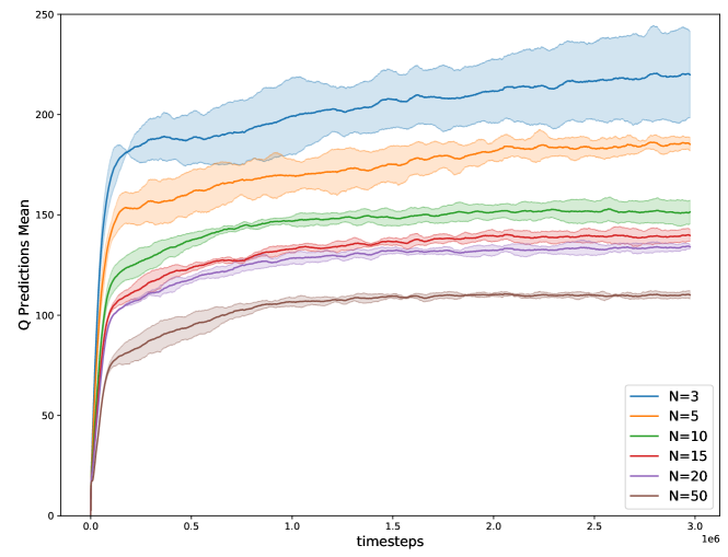
E.3 Conservatism of ensemble and SPQR

We visualize how ensemble size $N$ affects the conservatism, and how SPQR can be computationally effective. As we described in Section 4.1 and Figure 3, SPQR has conservatism power. Increasing ensemble size $N$ for SAC-Min shows conservative behavior, as proven in [22] and Figure 9. We train SAC-Min for 3M timesteps in a halfcheetah-random dataset with ensemble size $N=3,5,10,15,20,50$. SAC-Min empirically shows conservative behavior as ensemble size increases. As a result, SPQR can be a computationally efficient algorithm when using SAC-Min.

Refer to caption
Figure 9: Mean of predicted Q-value with various $N$, averaged over 4 seeds

E.4 Spike histogram visualization

We plot a more detailed visualization of the spike histogram for Figure 10. We visualize how the spike histogram of EDAC and SPQR varies compared with SAC-Min.

Refer to caption
Figure 10: Spike visualization for SAC-Min, EDAC, and SPQR-$\beta=0.01,0.1,1.0,10.0,100.0$.

E.5 Bias of Q

In Figure 11, we plot the average normalized bias and standard deviation of normalized bias. Bias is calculated by Monte-Carlo estimation. SPQR-$*$ decreases average bias and standard deviation of bias from baseline algorithms. For all environments, SPQR-SAC-Ens shows a smaller bias and standard deviation of bias than SAC-Ens. For Hopper and Humanoid tasks, SPQR-REDQ shows underestimation, and for Walker2d and Ant tasks, SPQR-REDQ shows unbiased estimation. For Ant, SPQR-REDQ shows less bias than REDQ.

Refer to caption
Figure 11: Average of bias and std of bias for SPQR-SAC-Ens and SPQR-REDQ, averaged over 4 seeds. G represents the UTD ratio.

E.6 UTD Ablation Study

We visualize the performance of SPQR-SAC-Ens over variation of UTD ratio in Figure 12. SPQR-SAC-Ens shows performance improvement by increasing the UTD ratio with a conservative and stable bias.

Refer to caption
Figure 12: Left 1: Average return of SPQR-SAC-Ens for UTD ratio 1,5, Left 2: Average of bias of SPQR-SAC-Ens for UTD ratio 1,5, Left 3: Standard deviation of bias of SPQR-SAC-Ens for UTD ratio 1,5. All experiments are averaged over 4 seeds. G represents the UTD ratio.

E.7 Early Collapse

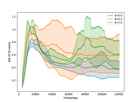
To show how SPQR affects the ensemble when the agent collects new tuple (s,a,r,sโ€ฒ)๐‘ ๐‘Ž๐‘Ÿsuperscript๐‘ โ€ฒ(s,a,r,s^{\prime}) in terms of exploration and variance, we evaluate the standard deviation with different $\beta$.

As [30] pointed out, the early collapse of Q-values occurs, which means that in an early stage of training, the variance of the Q-ensemble is almost zero since Q-values become similar to each other. To show how SPQR addresses the early collapse problem, we visualize the standard deviation of Q-ensemble in Figure 13. We train 10 Q-networks from the MuJoCo Hopper environment with the SAC-Min algorithm with the same hyperparameter. SPQR does not collapse Q-values during training, preserving appropriate variance of Q-value, and higher values of $\beta$ result in greater variance for $\beta=0.3$ and $\beta=2.0$.

Refer to caption
Figure 13: Standard deviation of Q-ensemble with different $\beta$, average over 3 seeds

E.8 Hyperparameter Sensitivity

We evaluate SPQR over various $\beta$ to demonstrate hyperparameter sensitivity. We fix $N=10$ for SPQR-SAC-Min and evaluate it on the D4RL Gym halfcheetah-random dataset and halfcheetah-medium dataset. Evaluation results are shown in Table 11.

Table 11: Performance of SPQR-SAC-Min over various $\beta$ on the D4RL halfcheetah-* dataset, averaged over 4 seeds
dataset $\beta=0.0$ $\beta=0.01$ $\beta=0.1$ $\beta=0.5$ $\beta=1.0$ $\beta=2.0$ $\beta=5.0$ $\beta=10.0$
random $28.0\pm 0.9$ $30.6\pm 3.4$ $32.4\pm 0.4$ $30.6\pm 1.3$ $30.7\pm 1.8$ $31.2\pm 2.2$ $31.1\pm 1.8$ $32.3\pm 2.4$
medium $67.5\pm 1.2$ $70.0\pm 0.5$ $71.7\pm 0.6$ $70.1\pm 1.0$ $70.5\pm 1.7$ $69.2\pm 1.3$ $70.0\pm 0.9$ $70.4\pm 1.3$

E.9 Compare with MED-RL

We implement and evaluate another diversifying method for online RL tasks, MED-RL. We use the Gini coefficient for MED-RL and use reported hyperparameters with UTD ratio 1. SPQR outperforms MED-RL for all tasks.

Refer to caption
Figure 14: Average returns of REDQ, SPQR-REDQ and MED-RL with UTD ratio 1 on the MuJoCo environment, averaged over 4 random seeds.

E.10 t-SNE Visualization

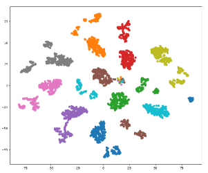
Figure 15 shows t-SNE [32] clustering visualization of Q-ensemble trained 3M timesteps by SPQR-SAC-Min algorithm at halfcheetah-medium-expert. We use t-SNE clustering for the last hidden layer representation of Q-ensemble with ensemble size 10 and 256 batch data at halfcheetah-medium-expert tasks. The t-SNE result shows that Q-ensemble trained by SPQR-SAC-Min is well clustered.

Refer to caption
Figure 15: t-SNE for SPQR-SAC-Min at halfcheetah-medium-expert

E.11 Correlation Visualization

We visualize a detailed figure for the Rightmost figure of Figure 1, the Pearson correlation coefficient matrix for a fully trained Q-ensemble and initial Q-ensemble in Figure 16. We train each Q-ensemble in the D4RL hopper-random dataset. For effective visualization, we sample randomly 10 Q-networks among 50 Q-networks and compute the Pearson correlation coefficient between each sampled Q-network with 256 batch data in a hopper-full-replay dataset. For the initial Q-ensemble, Q-networks are uncorrelated from each other. As we train Q-ensemble with SAC-Min for 3M timesteps, Q-networks become strongly correlated with each other.

Refer to caption
Refer to caption
Figure 16: Left: Q-ensemble trained 0 timesteps. Right: Q-ensemble trained 3M timesteps