Energy-efficient Decentralized Learning via Graph Sparsification

Abstract

This work aims at improving the energy efficiency of decentralized learning by optimizing the mixing matrix, which controls the communication demands during the learning process. Through rigorous analysis based on a state-of-the-art decentralized learning algorithm, the problem is formulated as a bi-level optimization, with the lower level solved by graph sparsification. A solution with guaranteed performance is proposed for the special case of fully-connected base topology and a greedy heuristic is proposed for the general case. Simulations based on real topology and dataset show that the proposed solution can lower the energy consumption at the busiest node by $54\%$–$76\%$ while maintaining the quality of the trained model.

1 Introduction

Learning from decentralized data [1] is an emerging machine learning paradigm that has found many applications [2].

Communication efficiency has been a major consideration in designing learning algorithms, as the cost in communicating model updates, e.g., communication time, bandwidth consumption, and energy consumption, dominates the total operation cost in many application scenarios [1]. Existing works on reducing this cost can be broadly classified into (i) model compression for reducing the cost per communication [3] and (ii) hyperparameter optimization for reducing the number of communications until convergence [4]. The two approaches are orthogonal and can be applied jointly.

In this work, we focus on hyperparameter optimization in the decentralized learning setting, where nodes communicate with neighbors according to a given base topology [5]. To this end, we adopt a recently proposed optimization framework from [6] that allows for systematic design of a critical hyperparameter in decentralized learning, the mixing matrix, to minimize a generally-defined cost measure. The choice of mixing matrix as the design parameter utilizes the observation from [7] that not all the links are equally important for convergence. Hence, instead of communicating over all the links at the same frequency as in most of the existing works [1, 4], communicating on different links with different frequencies can further improve the communication efficiency. However, the existing mixing matrix designs [7, 6] fall short at addressing a critical cost measure in wireless networks: energy consumption at the busiest node. Although energy consumption is considered in [6], its cost model only captures the total energy consumption over all the nodes. In this work, we address this gap based on a rigorous theoretical foundation.

1.1 Related Work

Decentralized learning algorithms. The standard algorithm for learning under a fully decentralized architecture was an algorithm called Decentralized Parallel Stochastic Gradient Descent (D-PSGD) [5], which was shown to achieve the same computational complexity but a lower communication complexity than training via a central server. Since then a number of improvements have been developed, e.g., [8], but these works only focused on the number of iterations.

Communication cost reduction. One line of works tried to reduce the amount of data per communication through model compression, e.g., [3]. Another line of works reduced the frequency of communications, e.g., [4]. Later works [9, 10] started to combine model compression and infrequent communications. Recently, it was recognized that better tradeoffs can be achieved by activating subsets of links, e.g., via event-based triggers [9, 10] or predetermined mixing matrices [7, 6]. Our work is closest to [7, 6] by also designing the mixing matrix, but we address a different objective of maximum per-node energy consumption.

Mixing matrix design. Mixing matrix design has been considered in the classical problem of distributed averaging, e.g., [11, 12] designed a mixing matrix with the fastest convergence to $\epsilon$-average and [13] designed a sequence of mixing matrices to achieve exact average in finite time. In contrast, fewer works have addressed the design of mixing matrices in decentralized learning [14, 7, 6, 15, 16]. Out of these, most focused on optimizing the training time, either by minimizing the time per iteration on computation [14] or communication [7, 15], or by minimizing the number of iterations [16]. To our knowledge, [6] is the only prior work that explicitly designed mixing matrices for minimizing energy consumption. However, [6] only considered the total energy consumption, but this work considers the energy consumption at the busiest node. Our design is based on an objective function that generalizes the spectral gap objective [17] to random mixing matrices. Spectral gap is an important parameter for capturing the impact of topology on the convergence rate of decentralized learning [5, 14]. Even if recent works identified some other parameters through which the topology can impact the convergence rate, such as the effective number of neighbors [17] and the neighborhood heterogeneity [16], their results did not invalidate the impact of spectral gap and just pointed out additional factors.

1.2 Summary of Contributions

We study the design of mixing matrix in decentralized learning with the following contributions:

1) Instead of considering the total energy consumption as in [6], our design aims at minimizing the energy consumption at the busiest node, leading to a more balanced load.

2) Instead of using a heuristic objective as in [7] or a partially justified objective as in [6], we use a fully theoretically-justified design objective, which enables a new approach for mixing matrix design based on graph sparsification.

3) Based on the new approach, we propose an algorithm with guaranteed performance for a special case and a greedy heuristic for the general case. Our solution achieves $54\%$–$76\%$ lower energy consumption at the busiest node while producing a model of the same quality as the best-performing benchmark in simulations based on real topology and dataset.

Roadmap. Section 2 formulates our problem, Section 3 presents the proposed solution, Section 4 evaluates it against benchmarks, and Section 5 concludes the paper. Proofs and additional evaluation results are provided in the appendix.

2 Background and Problem Formulation

2.1 Decentralized Learning Algorithm

Consider a network of $m$ nodes connected through a base topology $G=(V,E)$ ($|V|=m$), where $E$ defines the pairs of nodes that can directly communicate. Each node $i\in V$ has a local objective function $F_{i}(\bm{x})$ that depends on the parameter vector $\bm{x}\in\mathbb{R}^{d}$ and its local dataset. The goal is to minimize the global objective function $F(\bm{x}):=\frac{1}{m}\sum_{i=1}^{m}F_{i}(\bm{x}).$

We consider a state-of-the-art decentralized learning algorithm called D-PSGD [5]. Let $\bm{x}_{i}^{(k)}$ ($k\geq 1$) denote the parameter vector at node $i$ after $k-1$ iterations and $g(\bm{x}_{i}^{(k)};\xi_{i}^{(k)})$ the stochastic gradient computed in iteration $k$. D-PSGD runs the following update in parallel at each node $i$:

$$\bm{x}^{(k+1)}_{i}=\sum_{j=1}^{m}W^{(k)}_{ij}(\bm{x}^{(k)}_{j}-\eta g(\bm{x}^{(k)}_{j};\xi^{(k)}_{j})),$$ (1)

where $\bm{W}^{(k)}=(W^{(k)}_{ij})_{i,j=1}^{m}$ is the $m\times m$ mixing matrix in iteration $k$, and $\eta>0$ is the learning rate. To be consistent with the base topology, $W^{(k)}_{ij}\neq 0$ only if $(i,j)\in E$.

The convergence of this algorithm is guaranteed under the following assumptions:

1. Each local objective function $F_{i}(\bm{x})$ is $l$-Lipschitz smooth, i.e., $\|\nabla F_{i}(\bm{x})-\nabla F_{i}(\bm{x}^{\prime})\|\leq l\|\bm{x}-\bm{x}^{\prime}\|,\>\forall i\in V$.

2. There exist constants $M_{1},\hat{\sigma}$ such that ${1\over m}\sum_{i\in V}{\rm I\kern-2.70003ptE}[\|g(\bm{x}_{i};\xi_{i})-\nabla F_{i}(\bm{x}_{i})\|^{2}]\leq\hat{\sigma}^{2}+{M_{1}\over m}\sum_{i\in V}\|\nabla F(\bm{x}_{i})\|^{2}$, $\forall\bm{x}_{1},\ldots,\bm{x}_{m}\in\mathbb{R}^{d}$.

3. There exist constants $M_{2},\hat{\zeta}$ such that ${1\over m}\sum_{i\in V}\|\nabla F_{i}(\bm{x})\|^{2}\leq\hat{\zeta}^{2}+M_{2}\|\nabla F(\bm{x})\|^{2},\forall\bm{x}\in\mathbb{R}^{d}$.

Theorem 2.1.

[18, Theorem 2] Let $\bm{J}:={1\over m}\bm{1}\bm{1}^{\top}$. Under assumptions (1)–(3), if there exist a constant $p\in(0,1]$ such that the mixing matrices $\{\bm{W}^{(k)}\}_{k=1}^{K}$, each being symmetric with each row/column summing to one, satisfy

$${\rm I\kern-2.70003ptE}[\|\bm{X}\bm{W}^{(k)}-\bm{X}\bm{J}\|_{F}^{2}]\leq(1-p)\|\bm{X}-\bm{X}\bm{J}\|_{F}^{2},$$ (2)

for all $\bm{X}:=[\bm{x}_{1},\ldots,\bm{x}_{m}]$ and integer $k\geq 1$, then D-PSGD can achieve $\frac{1}{K}\sum_{k=1}^{K}\mathbbm{E}[\|\nabla F(\bm{\overline{x}}^{k})\|^{2}]\leq\epsilon_{0}$ for any given $\epsilon_{0}>0$ ($\overline{\bm{x}}^{(k)}:={1\over m}\sum_{i=1}^{m}\bm{x}^{(k)}_{i}$) when the number of iterations reaches

$$K(p) :=l(F(\overline{\bm{x}}^{(1)})-F_{\inf})$$

$$\cdot O\left({\hat{\sigma}^{2}\over m\epsilon_{0}^{2}}+{\hat{\zeta}\sqrt{M_{1}+1}+\hat{\sigma}\sqrt{p}\over p\epsilon_{0}^{3/2}}+{\sqrt{(M_{2}+1)(M_{1}+1)}\over p\epsilon_{0}}\right).$$

Remark: The required number of iterations $K(p)$ depends on the mixing matrix only through the parameter $p$: the larger $p$, the smaller $K(p)$. Originally, [18, Theorem 2] only mandates (2) for the product of $\tau$ mixing matrices, but we consider the case of $\tau=1$ for the tractability of mixing matrix design.

2.2 Mixing Matrix

As node $i$ needs to send its parameter vector to node $j$ in iteration $k$ only if $W^{(k)}_{ij}\neq 0$, we can control the communications by designing the mixing matrix $\bm{W}^{(k)}$. To this end, we use $\bm{W}^{(k)}:=\bm{I}-\bm{L}^{(k)},$ where $\bm{L}^{(k)}$ is the weighted Laplacian matrix [19] of the topology $G^{(k)}=(V,E^{(k)})$ activated in iteration $k$. Given the incidence matrix $\bm{B}$ of the base topology $G$ and a vector of link weights $\bm{\alpha}^{(k)}$, the Laplacian matrix $\bm{L}^{(k)}$ is given by $\bm{L}^{(k)}=\bm{B}\operatorname{diag}(\bm{\alpha}^{(k)})\bm{B}^{T}.$ The above reduces the mixing matrix design problem to a problem of designing the link weights $\bm{\alpha}^{(k)}$, where a link $(i,j)\in E$ will be activated in iteration $k$ if and only if $\alpha_{(i,j)}^{(k)}\neq 0$. This construction guarantees that $\bm{W}^{(k)}$ is symmetric with each row/column summing up to one.

2.3 Cost Model

We use $c(\bm{\alpha}^{(k)}):=(c_{i}(\bm{\alpha}^{(k)}))_{i=1}^{m}$ to denote the cost vector in an iteration when the link weight vector is $\bm{\alpha}^{(k)}$. We focus on the energy consumption at each node $i$, which contains two parts: (i) computation energy $c_{i}^{a}$ for computing the local stochastic gradient and the local aggregation, and (ii) communication energy $c_{ij}^{b}$ for sending the updated local parameter vector from node $i$ to node $j$. Then the energy consumption at node $i$ in iteration $k$ is modeled as

$$c_{i}(\bm{\alpha}^{(k)}):=c^{a}_{i}+\sum_{j:(i,j)\in E}c^{b}_{ij}\mathbbm{1}(\alpha_{(i,j)}^{(k)}\neq 0),$$ (3)

where $\mathbbm{1}(\cdot)$ denotes the indicator function. This cost function models the basic scenario where all communications are point-to-point and independent. Other scenarios are left to future work.

2.4 Optimization Framework

To trade off between the cost per iteration and the convergence rate, we adopt a bi-level optimization framework:

Lower-level optimization: design link weights $\bm{\alpha}$ to maximize the convergence rate (by maximizing $p$) under a given budget $\Delta$ on the maximum cost per node in each iteration, which results in a required number of iterations of $K(p_{\Delta})$.

Upper-level optimization: design $\Delta$ to minimize the total maximum cost per node ${\Delta}\cdot K(p_{\Delta})$.

3 Mixing Matrix Design via Graph Sparsification

As the upper-level optimization only involves one scalar decision variable, we will focus on the lower-level optimization.

3.1 Simplified Objective

The parameter $p$ that minimizes the required number of iterations $K(p)$ is given by

$$p:=\min_{\bm{X}\neq\bm{0}}\left(1-{{\rm I\kern-2.70003ptE}[\|\bm{X}(\bm{W}-\bm{J})\|_{F}^{2}]\over\|\bm{X}(\bm{I}-\bm{J})\|_{F}^{2}}\right).$$ (4)

As (4) is not an explicit function of the mixing matrix, we first relate it to an equivalent quantity that is easier to handle. We can relate $p$ to an explicit function of $\bm{W}$ as follows.

Lemma 3.1.

For any randomized mixing matrix $\bm{W}$ that is symmetric with every row/column summing to one, $p$ defined in (4) satisfies $p=1-\rho$ for $\rho:=\|{\rm I\kern-3.00003ptE}[\bm{W}^{\top}\bm{W}]-\bm{J}\|$.

Lemma 3.1 implies that the lower-level optimization should minimize $\rho$. While it is possible to formulate this minimization in terms of the link weights $\bm{\alpha}$, the resulting optimization problem, with a form similar to [6, (18)], will be intractable due to the presence of non-linear matrix inequality constraint. We thus further simplify the objective as follows.

Lemma 3.2.

For any mixing matrix $\bm{W}:=\bm{I}-\bm{L}$, where $\bm{L}$ is a randomized Laplacian matrix,

$$\rho \leq{\rm I\kern-2.70003ptE}\left[\|\bm{I}-\bm{L}-\bm{J}\|^{2}\right]$$ (5)

$$={\rm I\kern-2.70003ptE}\left[\max\left((1-\lambda_{2}(\bm{L}))^{2},(1-\lambda_{m}(\bm{L}))^{2}\right)\right],$$ (6)

where $\lambda_{i}(\bm{L})$ denotes the $i$-th smallest eigenvalue of $\bm{L}$.

By Lemma 3.2, we relax the objective of the lower-level optimization to designing a randomized $\bm{\alpha}$ by solving

$$\min_{\bm{\alpha}} \quad{\rm I\kern-2.70003ptE}\left[\|\bm{I}-\bm{B}\operatorname{diag}(\bm{\alpha})\bm{B}^{\top}-\bm{J}\|^{2}\right]$$ (7a)

s.t. $$\quad{\rm I\kern-2.70003ptE}[c_{i}(\bm{\alpha})]\leq\Delta,~{}~{}~{}\forall i\in V.$$ (7b)

3.2 Idea on Leveraging Graph Sparsification

We propose to solve the relaxed lower-level optimization (7) based on graph (spectral) sparsification. First, we compute the optimal link weight vector $\bm{\alpha}^{\prime}$ without the budget constraint (7b) by solving the following optimization:

$$\min_{\bm{\alpha}}\>\tilde{\rho}$$ (8a)

s.t. $$-\tilde{\rho}\bm{I}\preceq\bm{I}-\bm{B}\operatorname{diag}(\bm{\alpha})\bm{B}^{\top}-\bm{J}\preceq\tilde{\rho}\bm{I}.$$ (8b)

Constraint (8b) ensures $\tilde{\rho}=\|\bm{I}-\bm{B}\operatorname{diag}(\bm{\alpha})\bm{B}^{\top}-\bm{J}\|$ at the optimum, i.e., $\bm{\alpha}^{\prime}$ minimizes $\|\bm{I}-\bm{B}\operatorname{diag}(\bm{\alpha})\bm{B}^{\top}-\bm{J}\|$. Optimization (8) is a semi-definite programming (SDP) problem that can be solved in polynomial time by existing algorithms [20]. The vector $\bm{\alpha}^{\prime}$ establishes a lower bound on the relaxed objective: if $\bm{\alpha}^{*}$ is the optimal randomized solution for (7), then ${\rm I\kern-3.00003ptE}\left[\|\bm{I}-\bm{B}\operatorname{diag}(\bm{\alpha}^{*})\bm{B}^{\top}-\bm{J}\|^{2}\right]\geq\|\bm{I}-\bm{B}\operatorname{diag}(\bm{\alpha}^{\prime})\bm{B}^{\top}-\bm{J}\|^{2}$.

Then, we use a graph sparsification algorithm to sparsify the weighted graph with link weights $\bm{\alpha}^{\prime}$ to satisfy the budget constraint. As $\|\bm{I}-\bm{B}\operatorname{diag}(\bm{\alpha}^{\prime})\bm{B}^{\top}-\bm{J}\|^{2}$ $=\max\big{(}(1-\lambda_{2}(\bm{B}\operatorname{diag}(\bm{\alpha}^{\prime})\bm{B}^{\top}))^{2},$ $(1-\lambda_{m}(\bm{B}\operatorname{diag}(\bm{\alpha}^{\prime})\bm{B}^{\top}))^{2}\big{)}$, and graph sparsification aims at preserving the original eigenvalues $\left(\lambda_{i}(\bm{B}\operatorname{diag}(\bm{\alpha}^{\prime})\bm{B}^{\top})\right)_{i=1}^{m}$ [21], the sparsified link weight vector $\bm{\alpha}_{s}$ is expected to achieve an objective value $\|\bm{I}-\bm{B}\operatorname{diag}(\bm{\alpha}_{s})\bm{B}^{\top}-\bm{J}\|^{2}$ that approximates the optimal for (7).

3.3 Algorithm Design

We now apply the above idea to develop algorithms for mixing matrix design.

3.3.1 Ramanujan-Graph-based Design for a Special Case

Consider the special case when the base topology $G$ is a complete graph and all transmissions by a node have the same cost, i.e., $c_{ij}^{b}\equiv c_{i}^{b}$ for all $j$ such that $(i,j)\in E$. Let $d:=\min_{i\in V}\lfloor(\Delta-c_{i}^{a})/c_{i}^{b}\rfloor$. Then any graph with degrees bounded by $d$ satisfies the budget constraint. The complete graph has an ideal sparsifier known as Ramanujan graph. A $d$-regular graph $H$ is a Ramanujan graph if all the non-zero eigenvalues of its Laplacian matrix $\bm{L}_{H}$ lie between $d-2\sqrt{d-1}$ and $d+2\sqrt{d-1}$ [22]. By assigning weight ${1}/{d}$ to every link of a Ramanujan graph $H$, we obtain a weighted graph $H^{\prime}$, whose Laplacian $\bm{L}_{H^{\prime}}$ satisfies $\lambda_{1}(\bm{L}_{H^{\prime}})=0$ and

$$1-{2\sqrt{d-1}\over d}\leq\lambda_{2}(\bm{L}_{H^{\prime}})\leq\cdots\leq\lambda_{m}(\bm{L}_{H^{\prime}})\leq 1+{2\sqrt{d-1}\over d}.$$

By Lemma 3.2, the deterministic mixing matrix $\bm{W}_{H^{\prime}}:=\bm{I}-\bm{L}_{H^{\prime}}$ achieves a $\rho$-value $\rho_{H^{\prime}}$ that satisfies

$$\rho_{H^{\prime}} \leq\max\left((1-\lambda_{2}(\bm{L}_{H^{\prime}}))^{2},(1-\lambda_{m}(\bm{L}_{H^{\prime}}))^{2}\right)$$

$$\leq{4(d-1)\over d^{2}}=O\left({1\over d}\right)=O\left({1\over\Delta}\right).$$

Ramanujan graphs can be easily constructed by drawing random $d$-regular graphs until satisfying the Ramanujan definition [23]. By the result of [24], for $d\leq m^{1/3}$, we can generate random $d$-regular graphs in polynomial time. Thus, the above method can efficiently construct a deterministic mixing matrix with guaranteed performance in solving the lower-level optimization for a given budget $\Delta$ such that $d\leq m^{1/3}$.

3.3.2 Greedy Heuristic for General Case

For the general case, ideally we want to sparsify a weighted graph $G^{\prime}$ with link weights $\bm{\alpha}^{\prime}$ such that the sparsified graph with link weights $\bm{\alpha}_{s}$ will approximate the eigenvalues of $G^{\prime}$ while satisfying the constraint $c_{i}(\bm{\alpha}_{s})\leq\Delta$ for each $i\in V$. While this remains an open problem for general graphs, we propose a greedy heuristic based on the intuition that the importance of a link is reflected in its absolute weight. Specifically, we will find the link $(i,j)$ with the minimum absolute weight according to the solution to (8) such that the cost for either node $i$ or node $j$ exceeds the budget $\Delta$, set $\alpha_{(i,j)}=0$, and then find the next link by re-solving (8) under this additional constraint, until all the nodes satisfy the budget.

4 Performance Evaluation

We evaluate the proposed solution for the general case based on a real dataset and the topology of a real wireless network. We defer the evaluation in the special case to Appendix 5.2.

Experiment setting: We consider training for image classification based on CIFAR-10, which consists of 60,000 color images in 10 classes. We train the ResNet-50 model over its training dataset with 50,000 images, and then test the trained model over the testing dataset with 10,000 images. We use the topology of Roofnet [25] at data rate 1 Mbps as the base topology, which contains 33 nodes and 187 links. To evaluate the cost, we set the computation energy as $c^{a}_{i}=0.0003342$ (Wh) and the communication energy as $c^{b}_{ij}=0.0138$ (Wh) based on our parameters and the parameters from [26]. Following [6], we set the learning rate as 0.8 at the beginning and reduce it by 10X after 100, 150, 180, 200 epochs, and the mini-batch size to 32.

Benchmarks: We compare the proposed solution with with four benchmarks: ‘Vanilla D-PSGD’ [5] where all the neighbors communicate in all the iterations, ‘Periodic’ where all the neighbors communicate periodically, ‘MATCHA’ [7] which was designed to minimize training time, and Algorithm 1 in [6] (‘Greedy total’ or ‘Gt’ ) for the cost model (3) which was designed to minimize the total energy consumption. In ‘Vanilla D-PSGD’, ‘Periodic’, and ‘MATCHA’, identical weights are assigned to every activated link, whereas in ‘Greedy total’ and the proposed algorithm, heterogeneous link weights are parts of the designs. We first tune MATCHA to minimize its loss at convergence, and then tune the other benchmarks to activate the same number of links on the average. We evaluate two versions of the proposed algorithm (‘Greedy per-node’ or ‘Gp’): one with the same maximum energy consumption per node as the best-performing benchmark (leading to a budget that amounts to $55\%$ of maximum degree) and the other with the same accuracy as the best-performing benchmark at convergence (leading to a budget that amounts to $25\%$ of maximum degree).

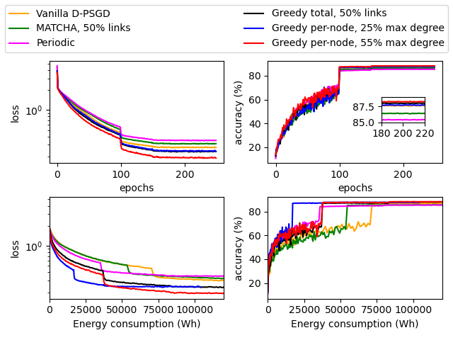
Fig. 1: Training loss and testing accuracy for decentralized learning over Roofnet.

Table 1: Stats at epoch 200.

Method	Loss	Acc.	Per-node Ene.	Total Ene.
Vanilla	0.277	87.6%	280kWh	4980kWh
Periodic	0.350	85.4%	140kWh	2490kWh
MATCHA	0.313	86.4%	213kWh	2490kWh
Gt, 50%	0.236	88.0%	147kWh	2477kWh
Gp, 25%	0.244	87.7%	67kWh	1465kWh
Gp, 55%	0.192	88.2%	147kWh	3169kWh

Results: Fig. 1 shows the loss and accuracy of the trained model, with respect to both the epochs and the maximum energy consumption per node. We see that: (i) instead of activating all the links as in ‘Vanilla D-PSGD’, it is possible to activate fewer (weighted) links without degrading the quality of the trained model; (ii) different ways of selecting the links to activate lead to different quality-cost tradeoffs; (iii) the algorithm designed to optimize the total energy consumption (‘Greedy total’) performs the best among the benchmarks; (iv) however, by balancing the energy consumption across nodes, the proposed algorithm (‘Greedy per-node’) can achieve either a better loss/accuracy at the same maximum energy consumption per node, or a lower maximum energy consumption per node at the same loss and accuracy. In particular, the proposed algorithm (at $25\%$ maximum degree) can save $54\%$ energy at the busiest node compared to the best-performing benchmark (‘Greedy total’) and $76\%$ compared to ‘Vanilla D-PSGD’, while producing a model of the same quality. Meanwhile, the proposed algorithm also saves $41$–$71\%$ of the total energy consumption compared to the benchmarks, as shown in Table 1.

5 Conclusion

Based on an explicit characterization of how the mixing matrix affects the convergence rate in decentralized learning, we proposed a bi-level optimization for mixing matrix design, with the lower level solved by graph sparsification. This enabled us to develop a solution with guaranteed performance for a special case and a heuristic for the general case. Our solution greatly reduced the energy consumption at the busiest node while maintaining the quality of the trained model.

Appendix

5.1 Supporting Proofs

Proof of Lemma 3.1.

One direction $p\leq 1-\rho$ was proved in [6], and we will prove that $p\geq 1-\rho$, or equivalently $1-p\leq\rho$. For this, we rely on the following fact (see [7, Lemma 1]): for any matrix $\bm{A}\in\mathbb{R}^{d\times m}$,

$${\rm I\kern-3.00003ptE}\left[\|\bm{A}(\bm{W}-\bm{J})\|_{F}^{2}\right]\leq\rho\|\bm{A}\|_{F}^{2}.$$ (9)

We fix a matrix $\bm{X}\neq 0$. Now set $\bm{A}=\bm{X}(\bm{I}-\bm{J})$, and (9) yields that

$$\frac{{\rm I\kern-3.00003ptE}\left[\|\bm{X}(\bm{I}-\bm{J})(\bm{W}-\bm{J})\|_{F}^{2}\right]}{\|\bm{X}(\bm{I}-\bm{J})\|_{F}^{2}}\leq\rho.$$ (10)

Note that for our choice of matrix $\bm{W}$, $\bm{WJ}=\bm{JW}=\bm{JJ}=\bm{J}$. Hence,

$$\bm{X}(\bm{I}-\bm{J})(\bm{W}-\bm{J})=\bm{X}(\bm{W}-\bm{J}-\bm{J}+\bm{J})=\bm{X}(\bm{W}-\bm{J}).$$ (11)

Thus, by (10) and (11), we establish that

$${{\rm I\kern-3.00003ptE}[\|\bm{X}(\bm{W}-\bm{J})\|_{F}^{2}]\over\|\bm{X}(\bm{I}-\bm{J})\|_{F}^{2}}\leq\rho.$$ (12)

Since $\bm{X}$ is an arbitrary nonzero matrix, it follows from (4) that $1-p\leq\rho$. ∎

Proof of Lemma 3.2.

As the spectral norm is convex, Jensen’s inequality implies

$$\rho:=\|{\rm I\kern-3.00003ptE}[\bm{W}^{\top}\bm{W}]-\bm{J}\|\leq{\rm I\kern-3.00003ptE}\|\bm{W}^{\top}\bm{W}-\bm{J}\|.$$ (13)

For a given Laplacian matrix $\bm{L}$,

$$\|\bm{W}^{\top}\bm{W}-\bm{J}\|=\|\bm{W}-\bm{J}\|^{2}=\|\bm{I}-\bm{L}-\bm{J}\|^{2},$$ (14)

where the first “$=$” is because the eigenvalues of $\bm{W}^{\top}\bm{W}-\bm{J}$ are squares of the eigenvalues of $\bm{W}-\bm{J}$ as shown by eigenvalue decomposition. By Lemma IV.2 in [6],

$$\|\bm{I}-\bm{L}-\bm{J}\|=\max\{1-\lambda_{2}(\bm{L}),\>\lambda_{m}(\bm{L})-1\},$$ (15)

Combining (13)–(15) yields (6). ∎

5.2 Additional Evaluation Results

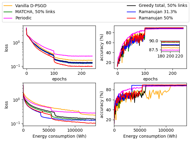
Fig. 2: Training loss and testing accuracy for decentralized learning over a complete graph.

In addition to the evaluation of the general case in Section 4, we also evaluate the special case of a fully-connected base topology. We use the same experiment setting and benchmarks as in Section 4, except that the base topology is a $33$-node complete graph. The proposed solution in this case is the Ramanujan-graph-based design in Section 3.3.1. We still evaluate two versions of this solution: one with the same maximum energy consumption per node as the best-performing benchmark (leading to a budget that amounts to $50\%$ of node degree in the base topology) and the other with an accuracy no worse than vanilla D-PSGD (leading to a budget that amounts to $31.3\%$ of node degree).

The results in Fig. 2 show that: (i) similar to Fig. 1, careful selection of the links to activate can notably improve the quality-cost tradeoff in decentralized learning; (ii) however, the best-performing benchmark under fully-connected base topology becomes ‘MATCHA’ even if it was designed for a different objective [7]; (iii) nevertheless, by intentionally optimizing a parameter (6) controlling the convergence rate while balancing the communication load across nodes, the proposed Ramanujan-graph-based solution can achieve a better loss/accuracy at the same maximum energy consumption per node (‘Ramanujan $50\%$’), or $37.5\%$ lower maximum energy consumption per node with a loss/accuracy no worse than ‘Vanilla D-PSGD’ (‘Ramanujan $31.3\%$’).

Compared with the results in Fig. 1, the proposed solution delivers less energy saving at the busiest node under a fully-connected base topology. Intuitively, this phenomenon is because the symmetry of the base topology leads to naturally balanced loads across nodes even if this is not considered by the benchmarks, which indicates that there is more room for improvement in cases with asymmetric base topology.

References

- [1] H. McMahan, Eider Moore, D. Ramage, S. Hampson, and Blaise Agüera y Arcas, “Communication-efficient learning of deep networks from decentralized data,” in AISTATS, 2017.
- [2] Peter Kairouz et al., Advances and Open Problems in Federated Learning, Now Foundations and Trends, 2021.
- [3] Anastasia Koloskova, Tao Lin, Sebastian U Stich, and Martin Jagg, “Decentralized deep learning with arbitrary communication compression,” in The International Conference on Learning Representations (ICLR), 2020.
- [4] Shiqiang Wang, Tiffany Tuor, Theodoros Salonidis, Kin K. Leung, Christian Makaya, Ting He, and Kevin Chan, “Adaptive federated learning in resource constrained edge computing systems,” IEEE Journal on Selected Areas in Communications, vol. 37, no. 6, pp. 1205–1221, 2019.
- [5] Xiangru Lian, Ce Zhang, Huan Zhang, Cho-Jui Hsieh, Wei Zhang, and Ji Liu, “Can decentralized algorithms outperform centralized algorithms? a case study for decentralized parallel stochastic gradient descent,” in Proceedings of the 31st International Conference on Neural Information Processing Systems, 2017, p. 5336–5346.
- [6] Cho-Chun Chiu, Xusheng Zhang, Ting He, Shiqiang Wang, and Ananthram Swami, “Laplacian matrix sampling for communication- efficient decentralized learning,” IEEE Journal on Selected Areas in Communications, vol. 41, no. 4, pp. 887–901, 2023.
- [7] J. Wang, A. K. Sahu, Z. Yang, G. Joshi, and S. Kar, “MATCHA: Speeding up decentralized SGD via matching decomposition sampling,” in NeurIPS Workshop on Federated Learning, 2019.
- [8] Yucheng Lu and Christopher De Sa, “Optimal complexity in decentralized training,” in International Conference on Machine Learning (ICML), 2021.
- [9] Navjot Singh, Deepesh Data, Jemin George, and Suhas Diggavi, “SPARQ-SGD: Event-triggered and compressed communication in decentralized optimization,” in IEEE CDC, 2020.
- [10] Navjot Singh, Deepesh Data, Jemin George, and Suhas Diggavi, “SQuARM-SGD: Communication-efficient momentum SGD for decentralized optimization,” IEEE Journal on Selected Areas in Information Theory, vol. 2, no. 3, pp. 954–969, 2021.
- [11] Lin Xiao and Stephen Boyd, “Fast linear iterations for distributed averaging,” Systems & Control Letters, vol. 53, pp. 65–78, September 2004.
- [12] Stephen Boyd, Arpita Ghosh, Balaji Prabhakar, and Devavrat Shah, “Randomized gossip algorithms,” in IEEE Transactions on Information Theory, 2006, vol. 52.
- [13] Julien M Hendrickx, Raphaël M Jungers, Alexander Olshevsky, and Guillaume Vankeerberghen, “Graph diameter, eigenvalues, and minimum-time consensus,” Automatica, pp. 635–640, 2014.
- [14] G. Neglia, G. Calbi, D. Towsley, and G. Vardoyan, “The role of network topology for distributed machine learning,” in IEEE INFOCOM, 2019.
- [15] Othmane Marfoq, Chuan Xu, Giovanni Neglia, and Richard Vidal, “Throughput-optimal topology design for cross-silo federated learning,” in Proceedings of the 34th International Conference on Neural Information Processing Systems, Red Hook, NY, USA, 2020, NIPS’20, Curran Associates Inc.
- [16] Batiste Le Bars, Aurélien Bellet, Marc Tommasi, Erick Lavoie, and Anne-Marie Kermarrec, “Refined convergence and topology learning for decentralized sgd with heterogeneous data,” in Proceedings of The 26th International Conference on Artificial Intelligence and Statistics, Francisco Ruiz, Jennifer Dy, and Jan-Willem van de Meent, Eds. 25–27 Apr 2023, vol. 206 of Proceedings of Machine Learning Research, pp. 1672–1702, PMLR.
- [17] Thijs Vogels, Hadrien Hendrikx, and Martin Jaggi, “Beyond spectral gap: the role of the topology in decentralized learning,” in Advances in Neural Information Processing Systems, S. Koyejo, S. Mohamed, A. Agarwal, D. Belgrave, K. Cho, and A. Oh, Eds. 2022, vol. 35, pp. 15039–15050, Curran Associates, Inc.
- [18] Anastasia Koloskova, Nicolas Loizou, Sadra Boreiri, Martin Jaggi, and Sebastian Stich, “A unified theory of decentralized SGD with changing topology and local updates,” in ICML, 2020.
- [19] Béla Bollobás, Modern Graph Theory, Graduate texts in mathematics. Springer, 2013.
- [20] Haotian Jiang, Tarun Kathuria, Yin Tat Lee, Swati Padmanabhan, and Zhao Song, “A faster interior point method for semidefinite programming,” in 2020 IEEE 61st Annual Symposium on Foundations of Computer Science (FOCS), 2020, pp. 910–918.
- [21] Daniel A. Spielman and Nikhil Srivastava, “Graph sparsification by effective resistances,” in ACM STOC, 2008.
- [22] Shlomo Hoory, Nathan Linial, and Avi Wigderson, “Expander graphs and their applications,” Bull. Amer. Math. Soc., vol. 43, no. 04, pp. 439–562, Aug. 2006.
- [23] Joel Friedman, “Relative expanders or weakly relatively Ramanujan graphs,” Duke Mathematical Journal, vol. 118, no. 1, pp. 19 – 35, 2003.
- [24] Jeong Han Kim and Van H. Vu, “Generating random regular graphs,” in Proceedings of the Thirty-Fifth Annual ACM Symposium on Theory of Computing, New York, NY, USA, 2003, STOC ’03, p. 213–222, Association for Computing Machinery.
- [25] Daniel Aguayo, John Bicket, Sanjit Biswas, Glenn Judd, and Robert Morris, “Link-level measurements from an 802.11b mesh network,” in SIGCOMM, 2004.
- [26] Xinchi Qiu, Titouan Parcollet, Javier Fernandez-Marques, Pedro P. B. Gusmao, Daniel J. Beutel, Taner Topal, Akhil Mathur, and Nicholas D. Lane, “A first look into the carbon footprint of federated learning,” 2021.