Accelerating non-local exchange in
generalized optimized Schwarz methods

X.Claeys Sorbonne Université, Laboratoire Jacques-Louis Lions R.Atchekzai Sorbonne Université, Laboratoire Jacques-Louis Lions CEA, CESTA
Abstract

The generalized optimised Schwarz method proposed in [Claeys & Parolin, 2022] is a variant of the Després algorithm for solving harmonic wave problems where transmission condition are enforced by means of a non-local exchange operator. We introduce and analyse an acceleration technique that significantly reduces the cost of applying this exchange operator without deteriorating the precision and convergence speed of the overall domain decomposition algorithm.

Introduction

The present article is concerned with the efficient numerical solution of time harmonic scalar wave equation by means of a substructuring domain decomposition method. In a recent series of contributions, we introduced variants of Després’ algorithm, also dubbed Optimized Schwarz Method (OSM), able to treat the presence of cross points in a systematic manner while maintaining geometric convergence of the overall DDM algorithms. This approach was proved a generalization of classical OSM in the sense that it coincides with it under appropriate circumstances. A full convergence framework was also provided for this new approach, including a precise quantification of convergence rates.

In classical OSM, wave equations are solved locally in each subdomain. The local solves are then coupled by means of a swapping operator $\Pi_{\mathrm{loc}}$ that exchanges ingoing/outgoing traces through each interface. In the generalized variant of OSM introduced in [4], a key innovation lies in a more sophisticated exchange operator $\Pi$ that replaces the swapping operator. While $\Pi_{\mathrm{loc}}$ is local by nature, the new exchange operator $\Pi$ is non-local because it a priori couples distant non-neighbouring subdomains (although $\Pi=\Pi_{\mathrm{loc}}$ in well identified circumstances).

Compared to the standard OSM, the generalized OSM leads to fastly converging DDM algorithms, but requires dealing with a potentially non-local exchange operator instead of the initial swapping operator, which represents an extra non-negligible computational cost. To be more precise, while the operation $\boldsymbol{x}\to\Pi_{\mathrm{loc}}(\boldsymbol{x})$ is trivial and simply consists in a permutation of unknowns, the operation $\boldsymbol{x}\to\Pi(\boldsymbol{x})$ requires the solution to a global problem that has nevertheless the favorable property of being hermitian positive definite. The goal of the present article is to exhibit one strategy that allows to perform the exchange operation $\boldsymbol{x}\to\Pi(\boldsymbol{x})$ approximately but much faster. We will prove in addition that this approximation does not induce any error in the overall DDM algorithm.

The exchange operation $\boldsymbol{x}\to\Pi(\boldsymbol{x})$ requires solving a self-adjoint positive definite (SPD) linear system, for which we rely on a preconditioned conjugate gradient (PCG) solver. At each iteration $n$ of the DDM algorithm, such a linear system $\mathrm{L}(\boldsymbol{x}^{(n)})=\boldsymbol{b}^{(n)}$ has to be solved. Two remarks can be made that allow to substantially accelerate these linear solves. First of all, the linear operator $\mathrm{L}$ is independent of $n$. Besides, the right hand sides $\boldsymbol{b}^{(n)}$ vary from one step $n$ to another, but they form a converging sequence because of the convergence of the overall DDM algorithm. In this context, our acceleration strategy consists in a simple recycling strategy combined with a brutal truncation of PCG (only a few iterations are needed). After a description of our method, we shall give numerical evidence of the performance of this approach. In the last of this contribution, we give a theoretical justification of the efficiency through derivation of an explicit convergence.

1 Scattering problem under study

We start by describing a typical wave propagation boundary value problem. The aim of the domain decomposition we are discussing here is to solve this problem as efficiently as possible. In the sequel $\Omega\subset\mathbb{R}^{d}$ will refer to a polygonal/polyhedral bounded domain, and we wish to solve the boundary value problem

$\displaystyle\text{Find}\;u\in\mathrm{H}^{1}(\Omega)\;\text{such that}$ (1)
$\displaystyle\Delta u+\kappa^{2}u=0\;\;\text{in}\;\Omega,$
$\displaystyle\partial_{\boldsymbol{n}}u-i\kappa u=f\;\;\text{on}\;\partial\Omega.$

where $f\in\mathrm{L}^{2}(\partial\Omega):=\{v:\Omega\to\mathbb{C},\;\|v\|_{\mathrm{L}^{2}(\partial\Omega)}^{2}:=\int_{\partial\Omega}|v|^{2}d\sigma<+\infty\}$ is any square integrable function and $\partial_{\boldsymbol{n}}u:=\boldsymbol{n}\cdot\nabla u$ with $\boldsymbol{n}$ the vector field normal to the boundary $\partial\Omega$ directed toward the exterior. The wave number is modelled as a real constant $\kappa>0$. Following widespread notations, we have considered the Sobolev space $\mathrm{H}^{1}(\Omega):=\{v\in\mathrm{L}^{2}(\Omega),\;\nabla v\in\mathrm{L}^{2}(\Omega)^{d}\}$ equipped with $\|v\|_{\mathrm{H}^{1}(\Omega)}^{2}:=\|\nabla v\|_{\mathrm{L}^{2}(\Omega)}^{2}+\kappa^{2}\|v\|_{\mathrm{L}^{2}(\Omega)}^{2}$. Problem (1) can be put in the variational form: find $u\in\mathrm{H}^{1}(\Omega)$ such that $a(u,v)=\ell(v)\;\forall v\in\mathrm{H}^{1}(\Omega)$ where

$$\begin{array}[]{rl}a(u,v)&\!\!\!:=\int_{\Omega}\nabla u\nabla\overline{v}-\kappa^{2}u\overline{v}\,d\boldsymbol{x}-i\kappa\int_{\partial\Omega}u\overline{v}\,d\sigma\\[5.0pt] \ell(v)&\!\!\!:=\int_{\partial\Omega}f\overline{v}\,d\sigma.\end{array}$$ (2)

Next we consider a regular triangulation $\mathcal{T}_{h}(\Omega)$ of the computational domain $\overline{\Omega}=\cup_{\tau\in\mathcal{T}_{h}(\Omega)}\overline{\tau}$ and we denote $\mathrm{V}_{h}(\Omega):=\{v\in\mathscr{C}^{0}(\overline{\Omega}):v|_{\tau}\in\mathbb{P}_{k}(\overline{\tau})\;\forall\tau\in\mathcal{T}_{h}(\Omega)\}\subset\mathrm{H}^{1}(\Omega)$ a space of $\mathbb{P}_{k}$-Lagrange finite element functions constructed on this mesh, where $\mathbb{P}_{k}(\overline{\tau}):=\{$ polynomials of order $\leq k$ on $\overline{\tau}$ $\}$.The associated discrete variational formulation then writes

$\displaystyle\text{Find}\;u_{h}\in\mathrm{V}_{h}(\Omega)\;\text{such that}$ (3)
$\displaystyle a(u_{h},v_{h})=\ell(v_{h})\;\;\forall v_{h}\in\mathrm{V}_{h}(\Omega).$

Problem (3) shall be assumed to admit a unique solution, which is simply equivalent to assuming that the corresponding matrix (for a given choice of shape functions) is invertible. The domain decomposition strategy that we subsequently discuss aims at computing this solution.

2 Decomposition of the computational domain

In the perspective of domain decomposition, we need to introduce a geometric decompositon of the computational domain. The strategy we wish to consider belongs to the class of substructuring methods and thus requires a non-overlapping partition of the computational domain

$\displaystyle\overline{\Omega}$ $\displaystyle=\overline{\Omega}_{1}\cup\dots\cup\overline{\Omega}_{\mathrm{J}}$ with $\displaystyle\;\;\Omega_{j}\cap\Omega_{k}=\emptyset\;\text{for}\;j\neq k,$ (4)
$\displaystyle\Sigma$ $\displaystyle=\Gamma_{1}\cup\dots\cup\Gamma_{\mathrm{J}}$ where $\displaystyle\;\;\Gamma_{j}:=\partial\Omega_{j}.$

Each $\Omega_{j}\subset\Omega$ will be a polyhedral assumed to be exactly resolved by the triangulation i.e. $\overline{\Omega}_{j}=\cup_{\tau\in\mathcal{T}_{h}(\Omega_{j})}\overline{\tau}$ where $\mathcal{T}_{h}(\Omega_{j}):=\{\tau\in\mathcal{T}_{h}(\Omega):\tau\subset\Omega_{j}\}$. Following usual parlance, we shall call $\Sigma$ the skeleton of the partition.

In practice the geometric decomposition above is obtained by means of a graph partitionner. Such a decomposition a priori involves cross-points i.e. points of adjacency of either three sub-domains or two sub-domains meeting and the exterior boundary. The set of cross-points is also refered to as wire basket in DDM related litterature. A major advantage of the DDM strategy we will consider is its ability to handle cross-points properly.

We consider finite element spaces local to each subdomain $\mathrm{V}_{h}(\Omega_{j}):=\{v_{h}|_{\Omega_{j}}:v_{h}\in\mathrm{V}_{h}(\Omega)\}$, as well as finite element spaces on local boundaries $\mathrm{V}_{h}(\Gamma_{j}):=\{v_{h}|_{\Gamma_{j}}:v_{h}\in\mathrm{V}_{h}(\Omega)\}$. We shall also refer to finite element functions defined on the skeleton

$$\mathrm{V}_{h}(\Sigma):=\{v_{h}|_{\Sigma}:\;v_{h}\in\mathrm{V}_{h}(\Omega)\}.$$ (5)

We also need to consider volume based finite element functions that are only piecewise continuous, with possible jumps through interfaces. Such a space is naturally identified with a cartesian product. This leads to setting

$$\mathbb{V}_{h}(\Omega):=\mathrm{V}_{h}(\Omega_{1})\times\dots\times\mathrm{V}_{h}(\Omega_{\mathrm{J}}).$$ (6)

We are interested in domain decomposition where behaviour of functions at interfaces play a crucial role, so we also need to introduce a space of traces at local boundaries $\mathbb{V}_{h}(\Sigma)$ and the corresponding trace map $\mathrm{B}:\mathbb{V}_{h}(\Omega)\to\mathbb{V}_{h}(\Sigma)$ defined by

$\displaystyle\mathbb{V}_{h}(\Sigma):=\mathrm{V}_{h}(\Gamma_{1})\times\dots\times\mathrm{V}_{h}(\Gamma_{\mathrm{J}})$ (7)
$\displaystyle\mathrm{B}(v):=(v_{1}|_{\Gamma_{1}},\dots,v_{\mathrm{J}}|_{\Gamma_{\mathrm{J}}}).$

Finally we need to embbed the space of trace on the skeleton into the space of traces on local boundaries by means of a restriction operator $\mathrm{R}:\mathrm{V}_{h}(\Sigma)\to\mathbb{V}_{h}(\Sigma)$ defined subdomain-wise through

$$\mathrm{R}(v):=(v|_{\Gamma_{1}},\dots,v|_{\Gamma_{\mathrm{J}}}).$$ (8)

The geometric decomposition that we have introduced above induces a decomposition of the sesquilinear form (2) and leads to an elementary reformulation of the discrete problem (3). Define $\mathrm{A}:\mathbb{V}_{h}(\Omega)\to\mathbb{V}_{h}(\Omega)^{*}$ and $\boldsymbol{l}\in\mathbb{V}_{h}(\Omega)^{*}$ by

$\displaystyle\langle\mathrm{A}(\boldsymbol{u}),\boldsymbol{v}\rangle$ $\displaystyle:=\sum_{j=1,\dots,\mathrm{J}}\int_{\Omega_{j}}\nabla u_{j}\nabla v_{j}-\kappa^{2}u_{j}v_{j}\,d\boldsymbol{x}-i\kappa\int_{\partial\Omega\cap\partial\Omega_{j}}u_{j}v_{j}d\sigma$ (9)
$\displaystyle\langle\boldsymbol{l},\boldsymbol{v}\rangle$ $\displaystyle:=\sum_{j=1,\dots,\mathrm{J}}\int_{\partial\Omega\cap\partial\Omega_{j}}f\,v_{j}\,d\boldsymbol{x}$

for any $\boldsymbol{u}=(u_{1},\dots,u_{\mathrm{J}}),\boldsymbol{v}=(v_{1},\dots,v_{\mathrm{J}})\in\mathbb{V}_{h}(\Omega)$. The operator $\mathrm{A}$ is block diagonal, with each block associated with a different subdomain. The initial discrete variational formulation can be rewritten as follows: a function $u_{h}\in\mathrm{V}_{h}(\Omega)$ solves (3) if and only if $\boldsymbol{u}=(u_{h}|_{\Omega_{1}},\dots,u_{h}|_{\Omega_{\mathrm{J}}})$ solves

$\displaystyle\boldsymbol{u}\in\mathbb{X}_{h}(\Omega):=\{(v|_{\Omega_{1}},\dots,v|_{\Omega_{\mathrm{J}}}),v\in\mathrm{V}_{h}(\Omega)\}$ (10)
$\displaystyle\text{and}\;\;\mathrm{A}(\boldsymbol{u}),\boldsymbol{v}\rangle=\langle\boldsymbol{l},\boldsymbol{v}\rangle\;\;\forall\boldsymbol{v}\in\mathbb{X}_{h}(\Omega).$

3 Exchange operator

To obtain a domain decomposition method, we need to further transform (10). Our final formulation will be posed in the function space $\mathbb{V}_{h}(\Sigma)$ attached to the skeleton, and we need to introduce a scalar product for this space i.e. an hermitian positive definite operator

$\displaystyle\mathrm{T}:\mathbb{V}_{h}(\Sigma)\to\mathbb{V}_{h}(\Sigma)^{*}\;\;\text{such that}$ (11)
$\displaystyle\mathrm{T}=\mathrm{T}^{*}\;\;\text{and}\;\;\langle\mathrm{T}(\boldsymbol{v}),\overline{\boldsymbol{v}}\rangle>0\;\forall\boldsymbol{v}\in\mathbb{V}_{h}(\Sigma)\setminus\{0\}.$

The operator $\mathrm{T}^{-1}:\mathbb{V}_{h}(\Sigma)^{*}\to\mathbb{V}_{h}(\Sigma)$ induces a scalar product on $\mathbb{V}_{h}(\Sigma)^{*}$. This scalar product will be used to quantify convergence of our domain decomposition algorithm. In the subsequent analysis, the space $\mathbb{V}_{h}(\Sigma)$ (resp. $\mathbb{V}_{h}(\Sigma)^{*}$) will be equipped with the norm

$\displaystyle\|\boldsymbol{v}\|_{\mathrm{T}}^{2}$ $\displaystyle:=\langle\mathrm{T}(\boldsymbol{v}),\overline{\boldsymbol{v}}\rangle$ (12)
$\displaystyle\|\boldsymbol{q}\|_{\mathrm{T}^{-1}}^{2}$ $\displaystyle:=\langle\mathrm{T}^{-1}(\boldsymbol{q}),\overline{\boldsymbol{q}}\rangle$

Based on the scalar products above, we are going to consider so-called exchange operators that are responsible for enforcing transmission conditions through interfaces and hence coupling between subdomains. We define the exchange operator $\Pi:\mathbb{V}_{h}(\Sigma)^{*}\to\mathbb{V}_{h}(\Sigma)^{*}$ by identity

$$\Pi:=2\mathrm{T}\mathrm{R}(\mathrm{R}^{*}\mathrm{T}\mathrm{R})^{-1}\mathrm{R}^{*}-\mathrm{Id}.$$ (13)

Because $\mathrm{T}\mathrm{R}(\mathrm{R}^{*}\mathrm{T}\mathrm{R})^{-1}\mathrm{R}^{*}$ is a $\mathrm{T}^{-1}$-orthogonal projector, it is clear that $\Pi$ is unitary by construction i.e. $\|\Pi(\boldsymbol{p})\|_{\mathrm{T}^{-1}}=\|\boldsymbol{p}\|_{\mathrm{T}^{-1}}\forall\boldsymbol{p}\in\mathbb{V}_{h}(\Sigma)^{*}$. Besides it is a priori non-local in the sense that it may couple trace function attached to distant subdomains.

4 Skeleton formulation

Now we describe a formulation equivalent to (10) that serves as the master equation of our domain decomposition algorithm. It will be posed on the skeleton of the decomposition. In this skeleton equation, wave problems local to each subdomain are written by means of a so-called scattering operator $\mathrm{S}:\mathbb{V}_{h}(\Sigma)^{*}\to\mathbb{V}_{h}(\Sigma)^{*}$ defined by

$\displaystyle\mathrm{S}:=\mathrm{Id}+2i\mathrm{T}\mathrm{B}(\mathrm{A}-i\mathrm{B}^{*}\mathrm{T}\mathrm{B})^{-1}\mathrm{B}^{*}$ (14)
$\displaystyle\boldsymbol{g}:=2i\mathrm{T}\mathrm{B}(\mathrm{A}-i\mathrm{B}^{*}\mathrm{T}\mathrm{B})^{-1}\boldsymbol{l}$

Since $\mathrm{A},\mathrm{B}$ are both subdomain-wise block-diagonal, when $\mathrm{T}$ is subdomain-wise block-diagonal, so is the scattering operator $\mathrm{S}$. This makes such an operator adapted to parallelism. The following Proposition was established in [2, Sec.6].

Proposition 4.1.

The tuple function $\boldsymbol{u}\in\mathbb{X}_{h}(\Omega)$ solves (10) if and only if there exists $\boldsymbol{q}\in\mathbb{V}_{h}(\Sigma)^{*}$ satisfying $\mathrm{B}^{*}\boldsymbol{q}=(\mathrm{A}-i\mathrm{B}^{*}\mathrm{T}\mathrm{B})\boldsymbol{u}-\boldsymbol{l}$ and the skeleton formulation

$\displaystyle\boldsymbol{q}\in\mathbb{V}_{h}(\Sigma)^{*}\;\text{and}$ (15)
$\displaystyle(\mathrm{Id}+\Pi\mathrm{S})\boldsymbol{q}=\boldsymbol{g}$

From the proposition above, we see that if the skeleton formulation (15) is solved, then the complete solution $\boldsymbol{u}=(\mathrm{A}-i\mathrm{B}^{*}\mathrm{T}\mathrm{B})^{-1}(\mathrm{B}^{*}\boldsymbol{q}+\boldsymbol{l})$ can be reconstructed, and this reconstruction step is fully parallel if the impedance operator $\mathrm{T}$ is block-diagonal.

A key feature of the skeleton formulation above is its strong coercivity with respect to the scalar product induced by $\mathrm{T}^{-1}$, in spite of the a priori sign indefiniteness of (10). The following result was established in [2, Cor. 6.2].

Proposition 4.2.

The operator $\mathrm{Id}+\Pi\mathrm{S}:\mathbb{V}_{h}(\Sigma)^{*}\to\mathbb{V}_{h}(\Sigma)^{*}$ is a bijection that fulfills a coercivity bound in the scalar product induced by $\mathrm{T}^{-1}$. For all $\boldsymbol{q}\in\mathbb{V}_{h}(\Sigma)^{*}$ we have

$\displaystyle\Re e\{\langle(\mathrm{Id}+\Pi\mathrm{S})\boldsymbol{q},\mathrm{T}^{-1}\overline{\boldsymbol{q}}\rangle\}\geq\frac{\gamma_{h}^{2}}{2}\|\boldsymbol{q}\|_{\mathrm{T}^{-1}}^{2}$
$\displaystyle\text{where}\;\;\gamma_{h}:=\mathop{\inf}_{\boldsymbol{q}\in\mathbb{V}_{h}(\Sigma)^{*}\setminus\{0\}}\|(\mathrm{Id}+\Pi\mathrm{S})\boldsymbol{q}\|_{\mathrm{T}^{-1}}/\|\boldsymbol{q}\|_{\mathrm{T}^{-1}}$

This result garantees a good behaviour of classical iterative solvers such as Richardson or GMRes when applied to the skeleton formulation (15). The coercivity estimate above leads to convergence bounds for such solvers, see e.g. [1].

In a Krylov solver, the matrix-vector operation $\boldsymbol{v}\mapsto(\mathrm{Id}+\Pi\mathrm{S})\boldsymbol{v}$ is a crucial step that has enormous impact on the computational cost of the overall solution procedure. In a situation where the impedance operator $\mathrm{T}$ is block-diagonal, the matrix-vector product $\boldsymbol{v}\mapsto\mathrm{S}\boldsymbol{v}$ is ambarassingly parallel as the scattering operator is itself block-diagonal.

As a consequence, the cost of the operation $\boldsymbol{v}\mapsto\Pi(\boldsymbol{v})$ is critical. This reduces to performing $\boldsymbol{v}\mapsto(\mathrm{R}^{*}\mathrm{T}\mathrm{R})^{-1}\boldsymbol{v}$ which, if performed in a naive way (like with a direct Cholesky solver), might be costly. Indeed solving a linear system attached to $\mathrm{R}^{*}\mathrm{T}\mathrm{R}$ is required each time a matrix-vector product is required inside the global Krylov solver.

The main goal of the present article is to show how this core step, that is at the center of our DDM strategy, can be optimized. We wish to exhibit how each such linear solve can benefit from the previous solves by means of a simple recycling strategies in such a way that the convergence speed of the overall DDM algorithm is not deteriorated.

For the sake of concreteness, we consider a Richardson solver, see e.g. Example 4.1 in [9], as a model iterative solver for the skeleton formulation (15). Starting from a trivial initial guess $\boldsymbol{q}^{(0)}=0$ and choosing $\alpha\in(0,1)$ as relaxation parameter, Richardson’s iteration takes the form

$$\boldsymbol{q}^{(n+1)}=(1-\alpha)\boldsymbol{q}^{(n)}-\alpha\Pi\mathrm{S}\boldsymbol{q}^{(n)}+\alpha\boldsymbol{g}.$$ (16)

Taking account of the expression of the exchange operator given by (13), this iteration can be decomposed as follows

$$\begin{array}[]{l}\textbf{Exact Richardson iteration}\\[5.0pt] \begin{aligned} \boldsymbol{p}^{(n+1)}&=(\mathrm{R}^{*}\mathrm{T}\mathrm{R})^{-1}\mathrm{R}^{*}\mathrm{S}\boldsymbol{q}^{(n)}\\ \boldsymbol{q}^{(n+1)}&=((1-\alpha)\mathrm{Id}+\alpha\mathrm{S})\boldsymbol{q}^{(n)}-2\alpha\mathrm{T}\mathrm{R}(\boldsymbol{p}^{(n+1)})+\alpha\boldsymbol{g}\end{aligned}\end{array}$$ (17)

We dub this algorithm "exact" because all steps in this procedure are assumed to be conducted without any error. In particular, it is assumed that no approximation is made when evaluating the action of $(\mathrm{R}^{*}\mathrm{T}\mathrm{R})^{-1}$ in the first line above.

5 Approximation of the exchange operator

In a large distributed memory environment, the linear solve of $\boldsymbol{q}\mapsto(\mathrm{R}^{*}\mathrm{T}\mathrm{R})^{-1}\boldsymbol{q}$ cannot be achieved exactly but should rely instead on an approximate PCG solve that consists in Galerkin projections onto a Krylov space that depends itself on the right hand side, see e.g. [7, §2.3].

Consider a linear map $\mathrm{P}:\mathrm{V}_{h}(\Sigma)^{*}\to\mathrm{V}_{h}(\Sigma)$ that, in the subsequent analysis, shall play the role of a preconditioner. For a given integer $k\geq 1$ and an initial guess $\boldsymbol{x}_{0}\in\mathrm{V}_{h}(\Sigma)$, define the $k$-th order Krylov space

$\displaystyle\mathscr{K}_{k}(\boldsymbol{b},\boldsymbol{x}_{0}):=\textrm{vect}\{\boldsymbol{r}_{0},(\mathrm{P}\mathrm{R}^{*}\mathrm{T}\mathrm{R})\boldsymbol{r}_{0},\dots,(\mathrm{P}\mathrm{R}^{*}\mathrm{T}\mathrm{R})^{k-1}\boldsymbol{r}_{0}\}$ (18)
$\displaystyle\text{where}\;\;\boldsymbol{r}_{0}:=\mathrm{P}\boldsymbol{b}-(\mathrm{P}\mathrm{R}^{*}\mathrm{T}\mathrm{R})\boldsymbol{x}_{0}.$

Define $\mathrm{PCG}_{k}:\mathrm{V}_{h}(\Sigma)\times\mathrm{V}_{h}(\Sigma)^{*}\to\mathrm{V}_{h}(\Sigma)$ as the map that takes a right-hand side $\boldsymbol{b}\in\mathrm{V}_{h}(\Sigma)^{*}$ and an initial guess $\boldsymbol{x}_{0}\in\mathrm{V}_{h}(\Sigma)$, and returns the result of $k$ steps of a PCG algorithm preconditionned with $\mathrm{P}$, see [9, §9.2]. Following the interpretation of Krylov methods in terms of projections, see [9, Chap.5 & 6] and [7, Chap.2], it is caracterised as the unique solution to the following minimization problem

$\displaystyle\mathrm{PCG}_{k}(\boldsymbol{x}_{0},\boldsymbol{b})\in\boldsymbol{x}_{0}+\mathscr{K}_{k}(\boldsymbol{x}_{0},\boldsymbol{b})\quad\text{and}$ (19)
$\displaystyle\|(\mathrm{R}^{*}\mathrm{T}\mathrm{R})^{-1}\boldsymbol{b}-\mathrm{PCG}_{k}(\boldsymbol{x}_{0},\boldsymbol{b})\|_{\mathrm{R}^{*}\mathrm{T}\mathrm{R}}=\min_{\eta\in\boldsymbol{x}_{0}+\mathscr{K}_{k}(\boldsymbol{x}_{0},\boldsymbol{b})}\|(\mathrm{R}^{*}\mathrm{T}\mathrm{R})^{-1}\boldsymbol{b}-\eta\|_{\mathrm{R}^{*}\mathrm{T}\mathrm{R}}.$

Let us see how the preconditioned conjugate gradient map $\mathrm{PCG}_{k}$ can be inserted into Richardson’s iteration (17). A naive approach would systematically take $\boldsymbol{x}_{0}=0$ as initial guess which leads to considering the relation $\boldsymbol{p}^{(n+1)}=\mathrm{PCG}_{k}(0,\mathrm{R}^{*}\mathrm{S}\boldsymbol{q}^{(n)})$ for the first equation in (17). However, because the overall DDM algorithm is supposed to converge, the right-hand sides $\mathrm{R}^{*}\mathrm{S}\boldsymbol{q}^{(n)}$ should themselve form a converging sequence. As a consequence $\mathrm{R}^{*}\mathrm{S}\boldsymbol{q}^{(n-1)}$ should remain close to $\mathrm{R}^{*}\mathrm{S}\boldsymbol{q}^{(n)}$, so that taking $\boldsymbol{x}_{0}=\boldsymbol{p}^{(n)}$ appears as a natural recycling strategy. The modified DDM strategy then takes the form

$$\begin{array}[]{l}\textbf{Approximate Richardson iteration}\\[5.0pt] \begin{aligned} \tilde{\boldsymbol{p}}^{(n+1)}&=\mathrm{PCG}_{k}(\tilde{\boldsymbol{p}}^{(n)},\mathrm{R}^{*}\mathrm{S}\tilde{\boldsymbol{q}}^{(n)})\\ \tilde{\boldsymbol{q}}^{(n+1)}&=((1-\alpha)\mathrm{Id}+\alpha\mathrm{S})\tilde{\boldsymbol{q}}^{(n)}-2\alpha\mathrm{T}\mathrm{R}(\tilde{\boldsymbol{p}}^{(n+1)})+\alpha\boldsymbol{g}\end{aligned}\end{array}$$ (20)

The parameter $k$ that represents the dimension of the Krylov space is assumed fixed and independent of $n$. Because the map $\mathrm{PCG}_{k}$ is not linear, we underline that the iterative procedure above is itself non-linear.

6 Numerical experiment

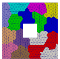
We now present a numerical experiment illustrating the strategy described above. We will consider Problem (1) set in $\mathbb{R}^{d}=\mathbb{R}^{2}$ in the computational domain $\Omega=(-1,+1)^{2}\setminus(-0.25,+0.25)^{2}$ represented below in Fig.1. We take $\lambda=1/10$ hence a wavenumber $\kappa=2\pi/\lambda\simeq 62.83$, and the source function $f(\boldsymbol{x})=\exp(i\kappa\,\boldsymbol{d}\cdot\boldsymbol{x})$ with $\boldsymbol{d}=(-1/\sqrt{2},+1/\sqrt{2},0)$. The problem is discretized with $\mathbb{P}_{1}$-Lagrange finite elements based on a mesh generated with gmsh and partitioned with metis in 16 subdomains. The computations were run sequentially with the C++ library ddmtool on a laptop with Intel® Core™ i7-1185G7 processor with 62.5 Gb of RAM.

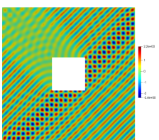
All the numerical experiments of the present section have been conducted with the same fixed mesh that contains 175794 nodes (which is also the dimension of $\mathrm{V}_{h}(\Omega)$) and 349588 triangles. The maximum mesh element size equals $h=0.005$ so this discretization represents approximately $\lambda/h=20$ points per wavelength. We compute a reference solution of (15) by means of a direct solver using umpfpack. This reference solution will be denoted $\boldsymbol{q}^{(\infty)}$ subsequently. Its real part is plotted in the right hand side of Figure 1 below.

Refer to caption
Refer to caption
Figure 1: Left: Computational domain. Right: Real part of the reference solution.

We construct the impedance operator $\mathrm{T}=\mathrm{diag}(\mathrm{T}_{1},\dots,\mathrm{T}_{\mathrm{J}}):\mathbb{V}_{h}(\Sigma)\to\mathbb{V}_{h}(\Sigma)^{*}$ following the strategy advocated in [8, Chap.8], [5], [3, §4.2]. In the present case, this boils down to selecting a subset of each subdomain $\tilde{\Omega}_{j}\subset\Omega_{j}$ consisting in 5 layers of elements neighbouring $\Gamma_{j}=\partial\Omega_{j}$ (in particular $\Gamma_{j}\subset\partial\tilde{\Omega}_{j}$) and defining each $\mathrm{T}_{j}:\mathrm{V}_{h}(\Gamma_{j})\to\mathrm{V}_{h}(\Gamma_{j})^{*}$ as the unique hermitian positive definite linear map satisfying the minimization property

$$\langle\mathrm{T}_{j}(v),v\rangle:=\min\{\;\|\tilde{v}\|_{\mathrm{L}^{2}(\tilde{\Omega}_{j})}^{2}+\kappa^{2}\|\tilde{v}\|_{\mathrm{L}^{2}(\tilde{\Omega}_{j})}^{2}+\kappa\|\tilde{v}\|_{\mathrm{L}^{2}(\partial\tilde{\Omega}_{j}\setminus\Gamma_{j})}^{2},\;\tilde{v}\in\mathrm{V}_{h}(\tilde{\Omega}_{j}),\;\tilde{v}|_{\Gamma_{j}}=v\}.$$

The actual evaluation of this impedance operator rests on a (sparse) Cholesky factorization performed by means of umfpack locally in each $\tilde{\Omega}_{j}$. As for the preconditioner $\mathrm{P}$ for the linear solve associated to the operation $\boldsymbol{b}\mapsto(\mathrm{R}^{*}\mathrm{T}\mathrm{R})^{-1}\boldsymbol{b}$, we choose the single level Neumann-Neumann preconditioner, see [6, §7.8.1] or [10, §6.2].

In a first experiment we run a variant of Algorithm (20) with $\alpha=1/2$, where the initial guess of PCG is chosen trivial i.e. we set $\tilde{\boldsymbol{p}}^{(n+1)}=\mathrm{PCG}_{k}(0,\boldsymbol{b})$ where $\boldsymbol{b}=\mathrm{R}^{*}\mathrm{S}\,\tilde{\boldsymbol{q}}^{(n)}$, and the PCG algorithm is executed until the relative residual error $\|\boldsymbol{b}-(\mathrm{R}^{*}\mathrm{T}\mathrm{R})\mathrm{PCG}_{k}(0,\boldsymbol{b})\|_{\mathrm{P}}/\|\boldsymbol{b}\|_{\mathrm{P}}\leq 1e-20$ is reached. In Figure 2 below, we plot the norm of the error $\|\boldsymbol{q}^{(\infty)}-\tilde{\boldsymbol{q}}^{(n)}\|_{\mathrm{T}^{-1}}/\|\boldsymbol{q}^{(\infty)}\|_{\mathrm{T}^{-1}}$ of Algorithm (20) versus the iteration number $n$.

Refer to caption
Refer to caption
Figure 2: Relative error $\|\boldsymbol{q}^{(\infty)}-\tilde{\boldsymbol{q}}^{(n)}\|_{\mathrm{T}^{-1}}/\|\boldsymbol{q}^{(\infty)}\|_{\mathrm{T}^{-1}}$ versus iteration number $n$ in Richardson’s Algorithm. No initial guess of PCG i.e. no recycling strategy. Left: no limitation on PCG iteration count i.e. $k_{\textsc{max}}=\infty$. Right: imposing in addition $k\leq k_{\textsc{max}}$.

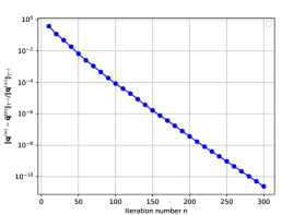
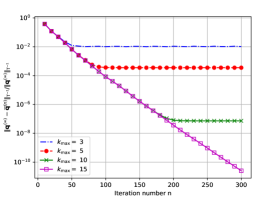
On the left picture of Fig.2, we take as many iterations of PCG as needed. For this plot, as a matter of fact, 14 iterations of PCG take place at each iteration of the global Richardson algorithm. On the right hand side of Fig.2, we plot the same graph except that this time the number of iterations of PCG is limited $k\leq k_{\textsc{max}}$ for several values of $k_{\textsc{max}}$. We see that when the number of PCG iterations is limited, the error $\|\boldsymbol{q}^{(\infty)}-\tilde{\boldsymbol{q}}^{(n)}\|_{\mathrm{T}^{-1}}/\|\boldsymbol{q}^{(\infty)}\|_{\mathrm{T}^{-1}}$ of the global Richardson algorithm decays normally until it reaches a certain critical value where it stalls. This plateau phenomenon appears here for $k_{\textsc{max}}<14$.

Next we launch the same computation, again limiting the number of PCG iterations $k\leq k_{\textsc{max}}$. This time though, we choose the initial guess from the previous iterate as described before i.e. $\tilde{\boldsymbol{p}}^{(n+1)}=\mathrm{PCG}_{k}(\boldsymbol{x}_{0},\boldsymbol{b})$ with $\boldsymbol{b}=\mathrm{R}^{*}\mathrm{S}\,\tilde{\boldsymbol{q}}^{(n)}$ and $\boldsymbol{x}_{0}=\tilde{\boldsymbol{p}}^{(n)}$. We do this for the two values $k_{\textsc{max}}=5$ and $k_{\textsc{max}}=10$ and plot the corresponding error $\|\boldsymbol{q}^{(\infty)}-\tilde{\boldsymbol{q}}^{(n)}\|_{\mathrm{T}^{-1}}/\|\boldsymbol{q}^{(\infty)}\|_{\mathrm{T}^{-1}}$ versus $n$. This time the error keeps on decaying without reaching any plateau.

Refer to caption
Figure 3: Relative error $\|\boldsymbol{q}^{(\infty)}-\tilde{\boldsymbol{q}}^{(n)}\|_{\mathrm{T}^{-1}}/\|\boldsymbol{q}^{(\infty)}\|_{\mathrm{T}^{-1}}$ versus iteration number $n$ in Richardson’s Algorithm with a recycled initial guess for PCG and $k\leq k_{\textsc{max}}=5,10$.

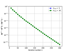
The plot of Fig.3 looks identical to the one in the left hand side of Fig.2. This suggests that, when combining a truncation of PCG with the simple recycling strategy described above, the error decay of the global Richardson algorithm does not experience any deterioration. Keeping this strategy consisting in both recycling and truncating PCG, in the next table, we give the number of iterations $n$ required to reach a relative tolerance $\|\boldsymbol{q}^{(\infty)}-\tilde{\boldsymbol{q}}^{(n)}\|_{\mathrm{T}^{-1}}/\|\boldsymbol{q}^{(\infty)}\|_{\mathrm{T}^{-1}}<1e-10$.

$k_{\textsc{max}}$ 20 15 10 5 3 2 1
$\#$iter 281 281 281 281 282 286 616

This clearly indicates that, when using a recycling strategy, only a few PCG iterations are needed to maintain the same convergence speed for the overall Richardson algorithm. This represents a clear computational gain since the cost of each iteration of (20) depends directly on $k_{\textsc{max}}$.

The previous result shows that, although the operator $\Pi$ is non-local, in practice its action may be evaluated with a cost corresponding to a small number of matrix-vector products from the operator $\mathrm{T}$. In the next section, we provide theoretical analysis supporting this conclusion.

7 Convergence analysis

We exhibited an efficient heuristic to approximate the action of the non-local exchange operator i.e. the first line in (17). It consists in combining a brutal truncation of PCG with a basic recycling scheme. We provided numerical evidence supporting the relevance of this strategy.

We seek now to obtain a theoretical explanation for the performance of this approach. Instead of trying to systematically derive the sharpest estimates, at certain points of our analysis we will take upper bounds that are larger than strictly required which, hopefully, will help simplify the calculus. To begin with, we re-arrange the approximate Richardson iteration (20),

$\displaystyle\tilde{\boldsymbol{p}}^{(n+1)}-\tilde{\boldsymbol{p}}^{(n+1)}_{\infty}=\mathrm{PCG}_{k}(\tilde{\boldsymbol{p}}^{(n)},\mathrm{R}^{*}\mathrm{S}\tilde{\boldsymbol{q}}^{(n)})-(\mathrm{R}^{*}\mathrm{T}\mathrm{R})^{-1}\mathrm{R}^{*}\mathrm{S}\tilde{\boldsymbol{q}}^{(n)}$ (21)
$\displaystyle\tilde{\boldsymbol{q}}^{(n+1)}=((1-\alpha)\mathrm{Id}-\alpha\Pi\mathrm{S})\tilde{\boldsymbol{q}}^{(n)}-2\alpha\mathrm{T}\mathrm{R}(\tilde{\boldsymbol{p}}^{(n+1)}-\tilde{\boldsymbol{p}}^{(n+1)}_{\infty})+\alpha\boldsymbol{g}$
$\displaystyle\text{where}\quad\tilde{\boldsymbol{p}}_{\infty}^{(n)}:=(\mathrm{R}^{*}\mathrm{T}\mathrm{R})^{-1}\mathrm{R}^{*}\mathrm{S}\tilde{\boldsymbol{q}}^{(n-1)}.$

Focusing on the first line of (21), we try to estimate the decay of the left hand side, making use of the classical convergence estimate for the conjugate gradient, see e.g. Corollary 5.6.7 in [7] that, in our notations, yields the following inequality

$\displaystyle\|(\mathrm{R}^{*}\mathrm{T}\mathrm{R})^{-1}\boldsymbol{b}-\mathrm{PCG}_{k}(\boldsymbol{x}_{0},\boldsymbol{b})\|_{\mathrm{R}^{*}\mathrm{T}\mathrm{R}}\leq\epsilon\|(\mathrm{R}^{*}\mathrm{T}\mathrm{R})^{-1}\boldsymbol{b}-\boldsymbol{x}_{0}\|_{\mathrm{R}^{*}\mathrm{T}\mathrm{R}}$ (22)
$\displaystyle\text{with}\;\;\epsilon=2\Big{(}\frac{\sqrt{\mathrm{cond}(\mathrm{P}\mathrm{R}^{*}\mathrm{T}\mathrm{R})}-1}{(\sqrt{\mathrm{cond}(\mathrm{P}\mathrm{R}^{*}\mathrm{T}\mathrm{R})}+1}\Big{)}^{k}$

and $\mathrm{cond}(\mathrm{L})$ refers to the spectral condition number i.e. $\mathrm{cond}(\mathrm{L})=\sup\mathfrak{S}(\mathrm{L})/\inf\mathfrak{S}(\mathrm{L})$ where $\mathfrak{S}(\mathrm{L})$ is the spectrum of a linear map $\mathrm{L}:\mathrm{V}_{h}(\Sigma)\to\mathrm{V}_{h}(\Sigma)$. For the moment, we assume that $k$ is chosen sufficiently large hence $\epsilon$ as small as required. We shall come back an discuss later on the choice of the parameter $k$. Injecting Estimate (22) into (21) leads to following inequality

$\displaystyle\|\tilde{\boldsymbol{p}}^{(n+1)}_{\infty}-\tilde{\boldsymbol{p}}^{(n+1)}\|_{\mathrm{R}^{*}\mathrm{T}\mathrm{R}}$ $\displaystyle\leq\epsilon\|\tilde{\boldsymbol{p}}^{(n+1)}_{\infty}-\tilde{\boldsymbol{p}}^{(n)}\|_{\mathrm{R}^{*}\mathrm{T}\mathrm{R}}$
$\displaystyle\leq\epsilon\|\tilde{\boldsymbol{p}}^{(n)}_{\infty}-\tilde{\boldsymbol{p}}^{(n)}\|_{\mathrm{R}^{*}\mathrm{T}\mathrm{R}}+\epsilon\|\tilde{\boldsymbol{p}}^{(n+1)}_{\infty}-\tilde{\boldsymbol{p}}^{(n)}_{\infty}\|_{\mathrm{R}^{*}\mathrm{T}\mathrm{R}}.$

By the very definition of the auxiliary variable in (21), we have $\tilde{\boldsymbol{p}}^{(n+1)}_{\infty}-\tilde{\boldsymbol{p}}^{(n)}_{\infty}=(\mathrm{R}^{*}\mathrm{T}\mathrm{R})^{-1}\mathrm{R}^{*}\mathrm{S}(\boldsymbol{w})$ where $\boldsymbol{w}=\tilde{\boldsymbol{q}}^{(n)}-\tilde{\boldsymbol{q}}^{(n-1)}$. On the other hand, since $\mathrm{T}\mathrm{R}(\mathrm{R}^{*}\mathrm{T}\mathrm{R})^{-1}\mathrm{R}^{*}$ is a $\mathrm{T}^{-1}$-orthogonal projection, and $\mathrm{S}$ is a contraction with respect to $\|\;\|_{\mathrm{T}^{-1}}$ according to Lemma 5.2 in [2], we have $\|\tilde{\boldsymbol{p}}^{(n+1)}_{\infty}-\tilde{\boldsymbol{p}}^{(n)}_{\infty}\|_{\mathrm{R}^{*}\mathrm{T}\mathrm{R}}=\|\mathrm{T}\mathrm{R}(\mathrm{R}^{*}\mathrm{T}\mathrm{R})^{-1}\mathrm{R}^{*}\mathrm{S}(\boldsymbol{w})\|_{\mathrm{T}^{-1}}\leq\|\boldsymbol{w}\|_{\mathrm{T}^{-1}}=\|\tilde{\boldsymbol{q}}^{(n)}-\tilde{\boldsymbol{q}}^{(n-1)}\|_{\mathrm{T}^{-1}}$. From this we obtain

$\displaystyle\|\tilde{\boldsymbol{p}}^{(n+1)}_{\infty}-\tilde{\boldsymbol{p}}^{(n+1)}\|_{\mathrm{R}^{*}\mathrm{T}\mathrm{R}}\leq\epsilon\|\tilde{\boldsymbol{p}}^{(n)}_{\infty}-\tilde{\boldsymbol{p}}^{(n)}\|_{\mathrm{R}^{*}\mathrm{T}\mathrm{R}}+\epsilon\|\tilde{\boldsymbol{q}}^{(n)}-\tilde{\boldsymbol{q}}^{(n-1)}\|_{\mathrm{T}^{-1}}.$ (23)

Coming back to the approximate Richardson iteration (21), we now focus on the second line. We take the difference of two successive iterates, which yields

$\displaystyle\tilde{\boldsymbol{q}}^{(n+1)}-\tilde{\boldsymbol{q}}^{(n)}$ $\displaystyle=((1-\alpha)\mathrm{Id}-\alpha\Pi\mathrm{S})(\tilde{\boldsymbol{q}}^{(n)}-\tilde{\boldsymbol{q}}^{(n-1)})$ (24)
$\displaystyle\phantom{=}-2\alpha\mathrm{T}\mathrm{R}(\tilde{\boldsymbol{p}}^{(n+1)}-\tilde{\boldsymbol{p}}^{(n+1)}_{\infty})+2\alpha\mathrm{T}\mathrm{R}(\tilde{\boldsymbol{p}}^{(n)}-\tilde{\boldsymbol{p}}^{(n)}_{\infty})$

Next we bound the norm of the left-hand side above, taking account of Inequality (23), and introducing the continuity modulus of $(1-\alpha)\mathrm{Id}-\alpha\Pi\mathrm{S}$ with respect to the norm induced by $\mathrm{T}^{-1}$. This yields

$\displaystyle\|\tilde{\boldsymbol{q}}^{(n+1)}-\tilde{\boldsymbol{q}}^{(n)}\|_{\mathrm{T}^{-1}}$ (25)
$\displaystyle\leq\rho\|\tilde{\boldsymbol{q}}^{(n)}-\tilde{\boldsymbol{q}}^{(n-1)}\|_{\mathrm{T}^{-1}}+2\alpha\|\tilde{\boldsymbol{p}}^{(n+1)}_{\infty}-\tilde{\boldsymbol{p}}^{(n+1)}\|_{\mathrm{R}^{*}\mathrm{T}\mathrm{R}}+2\alpha\|\tilde{\boldsymbol{p}}^{(n)}_{\infty}-\tilde{\boldsymbol{p}}^{(n)}\|_{\mathrm{R}^{*}\mathrm{T}\mathrm{R}}$
$\displaystyle\leq(\rho+2\alpha\epsilon)\|\tilde{\boldsymbol{q}}^{(n)}-\tilde{\boldsymbol{q}}^{(n-1)}\|_{\mathrm{T}^{-1}}+2\alpha(1+\epsilon)\|\tilde{\boldsymbol{p}}^{(n)}_{\infty}-\tilde{\boldsymbol{p}}^{(n)}\|_{\mathrm{R}^{*}\mathrm{T}\mathrm{R}}$
$\displaystyle\text{where}\quad\rho:=\sup_{\boldsymbol{q}\in\mathbb{V}_{h}(\Sigma)^{*}\setminus\{0\}}\frac{\|((1-\alpha)\mathrm{Id}-\alpha\Pi\mathrm{S})\boldsymbol{q}\|_{\mathrm{T}^{-1}}}{\|\boldsymbol{q}\|_{\mathrm{T}^{-1}}}.$

Now we can gather (23) and (25) to form a system of $2\times 2$ recursive inequalities. We slightly rescale the inequalities and apply the majorizations $\epsilon\leq 2\epsilon$ and $\alpha\leq 1$ to make the analysis more comfortable. Set

$$\mathfrak{R}:=\left[\begin{array}[]{cc}\rho+2\epsilon&2\sqrt{\epsilon(1+\epsilon)}\\ 2\sqrt{\epsilon(1+\epsilon)}&2\epsilon\end{array}\right],\quad\mathfrak{e}^{(n)}:=\left[\begin{array}[]{l}\|\tilde{\boldsymbol{q}}^{(n)}-\tilde{\boldsymbol{q}}^{(n-1)}\|_{\mathrm{T}^{-1}}\\ \|\tilde{\boldsymbol{p}}^{(n)}_{\infty}-\tilde{\boldsymbol{p}}^{(n)}\|_{\mathrm{R}^{*}\mathrm{T}\mathrm{R}}\sqrt{1+1/\epsilon}\end{array}\right].$$ (26)

Given two vectors of positive coefficients $u,v\in\mathbb{R}_{+}^{2}$ with $u=(u_{1},u_{2})$ and $v=(v_{1},v_{2})$, we shall write $u\leq v\iff u_{j}\leq v_{j}$ for $j=1,2$. With this notation we obtain $\mathfrak{e}^{(n+1)}\leq\mathfrak{R}\cdot\mathfrak{e}^{(n)}$. Iterating over $n$, since all coefficients are positive, we obtain $\mathfrak{e}^{(n)}\leq\mathfrak{R}^{n}\cdot\mathfrak{e}^{(0)}$ with $\mathfrak{e}^{(0)}=(\|\tilde{\boldsymbol{q}}^{(0)}\|_{\mathrm{T}^{-1}},0)^{\top}$. For $\boldsymbol{x}=(x_{1},x_{2})\in\mathbb{R}^{2}$, denoting $|\boldsymbol{x}|:=(|x_{1}|^{2}+|x_{2}|^{2})^{1/2}$ and the associated matrix norm $|\mathfrak{R}|=\sup_{\boldsymbol{x}\in\mathbb{R}^{2}\setminus\{0\}}|\mathfrak{R}\boldsymbol{x}|/|\boldsymbol{x}|$.

Lemma 7.1.

Under the condition that $|\mathfrak{R}|<1$, the sequence $\tilde{\boldsymbol{q}}^{(n)}$ defined by (20) converges toward $\boldsymbol{q}^{(\infty)}:=(\mathrm{Id}+\Pi\mathrm{S})^{-1}\boldsymbol{g}$ the solution to (15) and we have $\|\tilde{\boldsymbol{q}}^{(n)}-\boldsymbol{q}^{(\infty)}\|_{\mathrm{T}^{-1}}\leq\|\tilde{\boldsymbol{q}}^{(0)}\|_{\mathrm{T}^{-1}}\,|\mathfrak{R}|^{n+1}/(1-|\mathfrak{R}|)$ for all $n\geq 0$.

Proof:

First of all observe that $\|\tilde{\boldsymbol{q}}^{(n)}-\tilde{\boldsymbol{q}}^{(n-1)}\|_{\mathrm{T}^{-1}}\leq|\mathfrak{e}^{(n)}|\leq|\mathfrak{R}|^{n}\cdot|\mathfrak{e}^{(0)}|$. and $|\mathfrak{e}^{(0)}|=\|\tilde{\boldsymbol{q}}^{(0)}\|_{\mathrm{T}^{-1}}$. Now pick arbitrary integers $n,m$ with $m>n$. Under the assumption that $|\mathfrak{R}|<1$, we have the following estimate

$\displaystyle\|\tilde{\boldsymbol{q}}^{(m)}-\tilde{\boldsymbol{q}}^{(n)}\|_{\mathrm{T}^{-1}}$ $\displaystyle\leq\sum_{\nu=n+1}^{m}\|\tilde{\boldsymbol{q}}^{(\nu)}-\tilde{\boldsymbol{q}}^{(\nu-1)}\|_{\mathrm{T}^{-1}}\leq\|\tilde{\boldsymbol{q}}^{(0)}\|_{\mathrm{T}^{-1}}\sum_{\nu=n+1}^{m}|\mathfrak{R}|^{\nu}$ (27)
$\displaystyle\leq\|\tilde{\boldsymbol{q}}^{(0)}\|_{\mathrm{T}^{-1}}|\mathfrak{R}|^{n+1}/(1-|\mathfrak{R}|).$

This proves that the sequence $\tilde{\boldsymbol{q}}^{(n)}$ is of Cauchy type in the norm $\|\cdot\|_{\mathrm{T}^{-1}}$ and admits a limit that we denote $\tilde{\boldsymbol{q}}^{(\infty)}$. Letting $m\to\infty$ in (27) yields $\|\tilde{\boldsymbol{q}}^{(n)}-\tilde{\boldsymbol{q}}^{(\infty)}\|_{\mathrm{T}^{-1}}\leq\|\tilde{\boldsymbol{q}}^{(0)}\|_{\mathrm{T}^{-1}}|\mathfrak{R}|^{n+1}/(1-|\mathfrak{R}|)$, so there only remains to prove that $\tilde{\boldsymbol{q}}^{(\infty)}=\boldsymbol{q}^{(\infty)}$. Observe now that we also have

$$\|\tilde{\boldsymbol{p}}_{\infty}^{(n)}-\tilde{\boldsymbol{p}}^{(n)}\|_{\mathrm{R}^{*}\mathrm{T}\mathrm{R}}\leq\frac{|\mathfrak{e}^{(n)}|}{\sqrt{1+1/\epsilon}}\leq\frac{|\mathfrak{e}^{(0)}|\,|\mathfrak{R}|^{n}}{\sqrt{1+1/\epsilon}}$$

which proves that $\|\tilde{\boldsymbol{p}}_{\infty}^{(n)}-\tilde{\boldsymbol{p}}^{(n)}\|_{\mathrm{R}^{*}\mathrm{T}\mathrm{R}}\to 0$. Next, coming back to (20), recall that we have the relation $\tilde{\boldsymbol{q}}^{(n+1)}=((1-\alpha)\mathrm{Id}-\alpha\Pi\mathrm{S})\tilde{\boldsymbol{q}}^{(n)}-2\alpha\mathrm{T}\mathrm{R}(\tilde{\boldsymbol{p}}^{(n+1)}-\tilde{\boldsymbol{p}}^{(n+1)}_{\infty})+\alpha\boldsymbol{g}$. Taking $n\to\infty$ in the previous relation, we obtain that $\tilde{\boldsymbol{q}}^{(\infty)}$ satisfies the equation $\tilde{\boldsymbol{q}}^{(\infty)}=((1-\alpha)\mathrm{Id}-\alpha\Pi\mathrm{S})\tilde{\boldsymbol{q}}^{(\infty)}+\alpha\boldsymbol{g}$. After re-arrangement, this leads to $\tilde{\boldsymbol{q}}^{(\infty)}=(\mathrm{Id}+\Pi\mathrm{S})^{-1}\boldsymbol{g}=\boldsymbol{q}^{(\infty)}$, which ends the proof. $\Box$

A remarkable conclusion that can be drawn from the previous lemma is that, with recycling, truncation of the PCG algorithm for the computation of the exchange operator $\Pi$ does not induce any consistency error in the global DDM algorithm. Such is not the case when recycling is not used, as was shown through numerical experiments in the previous section.

Let us quantify more precisely the convergence rate. Because $\mathfrak{R}$ is symetric, its norm $|\mathfrak{R}|$ equals its spectral radius. As a consequence, to bound the convergence rate provided by the previous lemma, we need to estimate the largest eigenvalue of $\mathfrak{R}$. This can be done explicitely by examining its caracteristic polynomial.

$\displaystyle\mathrm{det}(\lambda\mathrm{Id}-\mathfrak{R})$ $\displaystyle=(\rho+2\epsilon-\lambda)(2\epsilon-\lambda)-4\epsilon(1+\epsilon)$
$\displaystyle=\lambda^{2}-\lambda(\rho+4\epsilon)-(2-\rho)2\epsilon$

Because $\rho<1$, we see that $(2-\rho)2\epsilon>0$ and that the roots of this polynomial have opposite signs. Hence $|\mathfrak{R}|$ agrees with the positive root. With the gross estimate $\sqrt{x+y}\leq\sqrt{x}+\sqrt{y}$, we deduce

$\displaystyle|\mathfrak{R}|$ $\displaystyle=\frac{1}{2}(\rho+4\epsilon)+\frac{1}{2}\sqrt{(\rho+4\epsilon)^{2}+8(2-\rho)\epsilon},$ (28)
$\displaystyle|\mathfrak{R}|$ $\displaystyle\leq\rho+4\epsilon+2\sqrt{\epsilon}.$

To simplify the above estimate observe that, if $\rho+4\sqrt{\epsilon}<1$, then $2\sqrt{\epsilon}<1\Rightarrow 4\epsilon<2\sqrt{\epsilon}$ and in this case $|\mathfrak{R}|\leq\rho+4\epsilon+2\sqrt{\epsilon}<\rho+4\sqrt{\epsilon}<1$. Let us examine what does the condition $\rho+4\sqrt{\epsilon}<1$ means. Recall that the operator $(1-\alpha)\mathrm{Id}-\alpha\Pi\mathrm{S}$ was proved to be a contraction, with the estimate $\rho\leq 1-\alpha(1-\alpha)\gamma_{h}^{2}$, see [4, Thm.9.2]. As a consequence, to ensure $\rho+4\sqrt{\epsilon}<1$, it is sufficient that

$$\epsilon=2\Big{(}\frac{\sqrt{\mathrm{cond}(\mathrm{P}\mathrm{R}^{*}\mathrm{T}\mathrm{R})}-1}{(\sqrt{\mathrm{cond}(\mathrm{P}\mathrm{R}^{*}\mathrm{T}\mathrm{R})}+1}\Big{)}^{k}<\big{(}\alpha(1-\alpha)\gamma_{h}^{2}/4\big{)}^{2}$$ (29)

Because $\epsilon$ decays exponentially fast to 00 as $k\to\infty$, which reflects the spectral convergence of the (preconditioned) conjugate gradient, only a few PCG iterations are necessary for satisfying (29). This is particularly true when the preconditioner $\mathrm{P}$ is devised appropriately. The next lemma summarizes the previous dsicussion on convergence criterion and convergence rate.

Lemma 7.2.

Assume the number $k$ of PCG iterations constant and chosen sufficiently large to satisfy Condition (29). Then $\rho+4\sqrt{\epsilon}<1$, and the sequence $\tilde{\boldsymbol{q}}^{(n)}$ defined by (20) converges toward $\boldsymbol{q}^{(\infty)}$ solution to (15) with the error estimate

$$\|\tilde{\boldsymbol{q}}^{(n)}-\boldsymbol{q}^{(\infty)}\|_{\mathrm{T}^{-1}}\leq\frac{\|\tilde{\boldsymbol{q}}^{(0)}\|_{\mathrm{T}^{-1}}}{1-(\rho+4\sqrt{\epsilon})}\;(\rho+4\sqrt{\epsilon})^{n}.$$

References

  • [1] B. Beckermann, S. A. Goreinov, and E. E. Tyrtyshnikov. Some remarks on the Elman estimate for GMRES. SIAM J. Matrix Anal. Appl., 27(3):772–778, 2006.
  • [2] X. Claeys. Non-self adjoint impedance in Generalized Optimized Schwarz Methods, 2021. preprint arXiv:2108.03652, to appear in IMA J.Num.An.
  • [3] X. Claeys, F. Collino, and E. Parolin. Nonlocal optimized Schwarz methods for time-harmonic electromagnetics. Adv. Comput. Math., 48(6):Paper No. 72, 36, 2022.
  • [4] X. Claeys and E. Parolin. Robust treatment of cross-points in Optimized Schwarz Methods. Numer. Math., 151(2):405–442, 2022.
  • [5] F. Collino, P. Joly, and E. Parolin. Non-local impedance operator for non-overlapping ddm for the helmholtz equation. In Domain Decomposition Methods in Science and Engineering XXVI, pages 725–733, Cham, 2022. Springer International Publishing.
  • [6] V. Dolean, P. Jolivet, and F. Nataf. An introduction to domain decomposition methods. Society for Industrial and Applied Mathematics (SIAM), Philadelphia, PA, 2015. Algorithms, theory, and parallel implementation.
  • [7] J. Liesen and Z. Strakoš. Krylov subspace methods. Numerical Mathematics and Scientific Computation. Oxford University Press, Oxford, 2013. Principles and analysis.
  • [8] E. Parolin. Non-overlapping domain decomposition methods with non-local transmissionoperators for harmonic wave propagation problems. Theses, Institut Polytechnique de Paris, December 2020.
  • [9] Y. Saad. Iterative methods for sparse linear systems. Philadelphia, PA: SIAM Society for Industrial and Applied Mathematics, 2nd ed. edition, 2003.
  • [10] A. Toselli and O. Widlund. Domain decomposition methods—algorithms and theory, volume 34 of Springer Series in Computational Mathematics. Springer-Verlag, Berlin, 2005.