LINKED FACTOR ANALYSIS

Abstract

Factor models are widely used in the analysis of high-dimensional data in several fields of research. Estimating a factor model, in particular its covariance matrix, from partially observed data vectors is very challenging. In this work, we show that when the data are structurally incomplete, the factor model likelihood function can be decomposed into the product of the likelihood functions of multiple partial factor models relative to different subsets of data. If these multiple partial factor models are linked together by common parameters, then we can obtain complete maximum likelihood estimates of the factor model parameters and thereby the full covariance matrix. We call this framework Linked Factor Analysis (LINFA). LINFA can be used for covariance matrix completion, dimension reduction, data completion, and graphical dependence structure recovery. We propose an efficient Expectation-Maximization algorithm for maximum likelihood estimation, accelerated by a novel group vertex tessellation (GVT) algorithm which identifies a minimal partition of the vertex set to implement an efficient optimization in the maximization steps. We illustrate our approach in an extensive simulation study and in the analysis of calcium imaging data collected from mouse visual cortex.

Keywords: EM algorithm; dimension reduction; graphical model; group vertex tessellation; matrix completion; maximum likelihood estimation; missing data.

1 Introduction

Factor analysis has been widely used to model high-dimensional data in neuroscience [9, 19, 47], psychology [36], psychometrics [6], econometrics [30, 1], financial econometrics [15, 18, 10], macroeconomics [42], and astrophysics [32, 26]. In a classical (Gaussian exploratory) factor analysis model we assume to observe $n$ independent and identically distributed (i.i.d.) $d$-dimensional random vectors $X_{1},\ldots,X_{n}$, generated according to the equation

$$X_{r}=\mu+\Lambda Z_{r}+\epsilon_{r},$$ (1.1)

where $\mu\in\mathbb{R}^{d}$ is the mean vector, $\Lambda\in\mathbb{R}^{d\times q}$ is the loading matrix, $Z_{1}$, …, $Z_{n}\stackrel{{\scriptstyle{\footnotesize\rm i.i.d.}}}{{\sim}}N(0,I_{q})$ are $q$-dimensional latent factors with identity covariance matrix, and $\epsilon_{1},\ldots,\epsilon_{n}\stackrel{{\scriptstyle{\footnotesize\rm i.i.d.}}}{{\sim}}N(0,\Psi)$ are $d$-dimensional error components with (diagonal) covariance matrix $\Psi$. Indeed, $X_{1},\ldots,X_{n}\stackrel{{\scriptstyle{\footnotesize\rm i.i.d.}}}{{\sim}}N(\mu,\Sigma)$, where

$$\Sigma=\Lambda\Lambda^{\mathrm{T}}+\Psi$$ (1.2)

is a $d\times d$ covariance matrix, and $\Lambda\Lambda^{\mathrm{T}}$ is a $d\times d$ matrix with rank no larger than $q$. The parameters $\mu$, $\Lambda$, and $\Psi$ of the factor model can be estimated in various ways, including maximum likelihood estimation [4, 17], penalized maximum likelihood estimation [14, 44, 23, 13], and Bayesian methods [7, 24, 35, 39].

Factor models are very attractive from the estimation point of view, because the number of parameters involved can be maintained substantially low even for very large $d$. Indeed, the total number of parameters that characterize the covariance matrix $\Sigma$ in Equation (1.2) is $d(q+1)$, so if $q<(d-1)/2$, then it can be very much smaller than the full dimensionality $d(d+1)/2$ of an unconstrained covariance matrix. This property is especially useful in the high-dimensional setting since, for a fixed number of factors $q$, the total number of parameters in a factor model increases only linearly with $d$, while in the unconstrained case it increases quadratically. However, Equation (1.2) is notoriously affected by a rotational invariance problem: for any $q\times q$ orthogonal matrix $P$, we have that $\tilde{\Lambda}=\Lambda P$ yields the same covariance matrix $\Sigma=\tilde{\Lambda}\tilde{\Lambda}^{\mathrm{T}}+\Psi$ simply because $\Lambda\Lambda^{\mathrm{T}}=\tilde{\Lambda}\tilde{\Lambda}^{\mathrm{T}}$. With no appropriate constraints, any estimation algorithm would yield one of infinitely many possible estimates of $\Lambda$ [3, 27, 4]. However, the covariance matrix $\Sigma$ in Equation (1.2) ultimately is not affected by the rotational invariance dilemma because the loading matrix $\Lambda$ simply acts as a nuisance parameter in Equation (1.2) [7]. The focus of our work is the estimation of $\Sigma$, so the rotation problem plays a minor role in our methodology. Nonetheless, in our estimation algorithms, we apply the simple but effective constraint of $\Lambda^{\mathrm{T}}\Psi^{-1}\Lambda$ being a diagonal matrix with diagonal entries in decreasing order [4]. This constrain allows us to identify $\Lambda$ up to a sign flip.

In this paper we investigate the problem of estimating a factor model in case of structural or deterministic missingness, where the data vectors $X_{1},\ldots,X_{n}$ are not fully observed because of technological constraints, in which case several pairs of variables may even have no joint data observation. For example, in neuroscience it is often impossible to record the activity of an entire population of neurons simultaneously with a reasonable temporal resolution. Instead, smaller subsets of neurons are usually recorded simultaneously over independent experimental sessions using a fine temporal resolution. These settings, however, yield $K$ data sets about the activity of $K$ different subsets of neurons, and several pairs of neurons may never be recorded jointly. Structural or deterministic missingness profoundly differs from typical missing-data problems [12, 11, 28, 25, 40, 38], such as missingness at random and variants, where each variable pair may be observed at least a few times with high-probability. The type of structural missingness we deal with has been investigated outside of factor modeling, such as in the context of sparse precision matrix estimation [46], and recovery of exact low rank positive semidefinite matrices [8].

We tackle the problem of estimating a factor model, in particular the covariance matrix $\Sigma$ in Equation (1.2), from structurally incomplete data as follows. In Section 2, we note that the likelihood function of the observed data can be factorized into the product of the likelihood functions of multiple partial factor models that are linked together by shared portions of the loading matrix $\Lambda$ and $\Psi$. Maximum likelihood estimation can be implemented efficiently to estimate the components $(\Lambda,\Psi)$ in Equation (1.2), and thereby $\Sigma$. We call this modeling framework Linked Factor Analysis, or LINFA. In Section 3, we propose an Expectation-Maximization (EM) algorithm for the computation of the maximum likelihood estimator $(\hat{\Lambda},\hat{\Psi})$ of the parameters $(\Lambda,\Psi)$. The EM algorithm has been implemented for factor models also in, for example, [48], [37], and [5]. However, [48] assumed complete data observations, [37] considered missing data but assumed the loading matrix $\Lambda$ to be known, and [5] dealt with arbitrary missing data patterns but used the Kalman filter to approximate the various conditional expectations involved in the expectation step. Our LINFA EM algorithm can also be applied to data with arbitrary missingness patterns, and involves conditional expectations and updating equations all in closed form. Furthermore, the maximization step of our proposed EM algorithm is accelerated by a novel Group Vertex Tessellation (GVT) algorithm, which identifies a minimal partition of the vertex set to implement an efficient circular optimization in the maximization steps. The GVT algorithm is very fast and needs to be run only once before the EM algorithm is executed.

In Section 4 we demonstrate in simulations that LINFA can be effectively used for covariance matrix completion, dimension reduction, data completion, and graphical dependence structure recovery, and our proposed EM algorithm with GVT acceleration is computationally efficient. In Section 5 we apply the methods to the analysis of calcium imaging data collected from mouse visual cortex, and finally, in Section 6, we discuss our results and future research directions.

2 The Linked Factor Analysis Model

Assume the generative factor model in Equation (1.1), and suppose we observe $K$ independent data matrices $\mathbf{X}^{(1)},\ldots,\mathbf{X}^{(K)}$, where $\mathbf{X}^{(k)}\in\mathbb{R}^{n_{k}\times|V_{k}|}$ contains $n_{k}$ independent and identically distributed samples $X_{1}^{(k)},\ldots,X_{n_{k}}^{(k)}$ about variables in the set $V_{k}$, where $V_{1},\ldots,V_{K}\subset V=\{1,\ldots,d\}$ with $|V_{k}|>1$ for all $k=1,\ldots K$, and $\cup_{k=1}^{K}V_{k}=V=\{1,\ldots,d\}$. Indeed,

$$X_{r}^{(k)}=\mu^{(k)}+\Lambda^{(k)}Z_{r}+\epsilon_{r}^{(k)},~{}~{}~{}~{}r=1,\ldots,n_{k},~{}k=1,\ldots,K,$$ (2.1)

where $\mu^{(k)}=(\mu_{j})_{j\in V_{k}}$, $\Lambda^{(k)}=[\Lambda_{ij}]_{i\in V_{k},j\in\{1,\ldots,q\}}$, $\epsilon_{1}^{(k)},\ldots,\epsilon_{n_{k}}^{(k)}\stackrel{{\scriptstyle{\footnotesize\rm i.i.d.}}}{{\sim}}N(0,\Psi_{V_{k}})$, and $\Psi^{(k)}=[\Psi_{ij}]_{i,j\in V_{k}}$. Thus, $X_{r}^{(k)}\sim N(0,[\Lambda\Lambda^{\mathrm{T}}+\Psi]_{V_{k},V_{k}})$, where $[\Lambda\Lambda^{\mathrm{T}}+\Psi]_{V_{k},V_{k}}=\Lambda^{(k)}\Lambda^{(k){\mathrm{T}}}+\Psi^{(k)}$. For simplicity, we shall assume $\mu=0$. We further assume that the observational pattern is structural and independent of any random variable in the system. Therefore, the likelihood function of the observed data $\mathbf{X}^{(1)},\ldots,\mathbf{X}^{(K)}$ takes the form

$$L(\Lambda,\Psi;\mathbf{X}^{(1)},\ldots,\mathbf{X}^{(K)})~{}=~{}\prod_{k=1}^{K}L_{k}(\Lambda^{(k)},\Psi^{(k)};\mathbf{X}^{(k)}),$$ (2.2)

where $L_{k}(\Lambda^{(k)},\Psi^{(k)};\mathbf{X}^{(k)})$ is the Gaussian likelihood function for the data set $\mathbf{X}^{(k)}$. If $V_{1},\ldots,V_{K}$ overlap sufficiently, then the $K$ likelihood functions in Equation (2.2) are linked together by the shared portions of parameters $\Lambda$ and $\Psi$, so inference based on their product will yield appropriate full estimates of $\Lambda$ and $\Psi$. For example, suppose $d=100$ and $K=2$, with $V_{1}=\{1,\ldots,80\}$ and $V_{2}=\{21,\ldots,100\}$. Then, $\Lambda^{(1)}$ and $\Lambda^{(2)}$ share the components $\Lambda_{ij}$ of $\Lambda$ for $i\in\{21,\ldots,80\}$ and $j=1,\ldots,q$, and $\Psi^{(1)}$ and $\Psi^{(2)}$ share the diagonal entries $\Psi_{ii}$ of $\Psi$ for $21\leq i\leq 80$. In Section 3 we propose an expectation-maximization algorithm for the computation of the maximum likelihood estimators $(\hat{\Lambda},\hat{\Psi})$ of $(\Lambda,\Psi)$.

LINFA is a unified framework for covariance matrix completion, dimension reduction, data completion and graphical dependence structure recovery in the case where the data suffer from structural missingness. Indeed, given the maximum likelihood estimates $(\hat{\Lambda},\hat{\Psi})$, the LINFA covariance matrix estimate is given by

$$\hat{\Sigma}=\hat{\Lambda}\hat{\Lambda}^{\mathrm{T}}+\hat{\Psi}$$ (2.3)

Moreover, dimension reduction can be performed by predicting the latent factors as

$$\hat{Z}_{r}^{(k)}~{}=~{}\hat{\Lambda}^{(k){\mathrm{T}}}\hat{\Sigma}^{(k)-1}X_{r}^{(k)}$$ (2.4)

where $\hat{\Lambda}^{(k)}$ is the estimate of $\Lambda^{(k)}$, $\hat{\Sigma}^{(k)}=\hat{\Sigma}_{V_{k}V_{k}}$, and $X_{r}\in\mathbb{R}^{|V_{k}|}$ is the $r$-th sample in $\mathbf{X}^{(k)}$. Furthermore, data completion can then be implemented by using the relevant predicted entries in the vectors

$$\hat{X}_{r}=\hat{\Lambda}\hat{Z}_{r}^{(k)}$$ (2.5)

Finally, in our framework, conditional dependence can be studied in two ways: (a) unconditionally on the factors and (b) conditionally on the factors. In case (a), we study the partial correlations between variable pairs $(X_{ri},X_{rj})$,

$$\rho_{ij}~{}:=~{}{\rm Cor}(X_{ri},X_{rj}\mid\{X_{rh}\}_{h\notin\{i,j\}})~{}=~{}-\frac{\Theta_{ij}}{\sqrt{\Theta_{ii}\Theta_{jj}}},~{}~{}~{}\text{for}~{}1\leq i<j\leq d$$ (2.6)

where $\Theta=\Sigma^{-1}$ can be computed efficiently via Woodbury Matrix Identity

$$\Theta~{}=~{}\Psi^{-1}-\Psi^{-1}\Lambda(I+\Lambda^{\mathrm{T}}\Psi^{-1}\Lambda)^{-1}\Lambda^{\mathrm{T}}\Psi^{-1},$$ (2.7)

Then, a partial correlation graph will contain $d$ nodes representing the variables $X_{r1},\ldots,X_{rd}$, and an edge connects nodes $(i,j)$ with strength proportional to the magnitude of $\rho_{ij}\in[-1,1]$. In case (b), we compute the conditional correlations

$$\gamma_{ij}~{}=~{}{\rm Cor}(X_{ri},Z_{rj}\mid\{Z_{rh}\}_{h\neq j})~{}=~{}\frac{\Lambda_{ij}}{\sqrt{\Lambda_{ij}^{2}+\Psi_{ii}}},~{}~{}~{}\text{for}~{}1\leq i\leq d,1\leq j\leq q$$ (2.8)

Then, we can construct a factor graph with $d$ nodes representing the variables $X_{r1},\ldots,X_{rd}$ and $q$ nodes representing the latent factors $Z_{r1},\ldots,Z_{rd}$, and an edge connects a variable node $X_{ri}$ and a latent node $Z_{rj}$ with strength proportional to the magnitude of $\gamma_{ij}\in[-1,1]$. No edge connects any two variables $X_{ri},X_{rj}$ or any two latent factors $Z_{ri},Z_{rj}$.

We investigate all these applications of LINFA in Section 4.

Figure 1: Latent factors and observed variables. LINFA lets us learn the parameters of the factor model (Equation (1.2)) from partially observed random vectors.

3 Maximum Likelihood Estimation

In this section we present an expectation-maximization algorithm to compute the maximum likelihood estimators of $\Lambda$ and $\Psi$,

$$(\hat{\Lambda},\hat{\Psi})~{}=~{}\underset{\Lambda\in\mathbb{R}^{d\times q},\Psi\in\mathcal{D}^{d\times d}_{++}}{\arg\max}L(\Lambda,\Psi;\mathbf{X}^{(1)},\ldots,\mathbf{X}^{(K)}),$$ (3.1)

where $L(\Lambda,\Psi;\mathbf{X}^{(1)},\ldots,\mathbf{X}^{(K)})$ is the likelihood function defined in Equation (2.2), and $\mathcal{D}^{d\times d}_{++}$ is the set of $d\times d$ positive diagonal matrices. Our algorithm can also be applied to data with arbitrary missingness patterns, and involves conditional expectations and updating equations all in closed form. Furthermore, the maximization step of our proposed EM algorithm is accelerated by the novel Group Vertex Tessellation (GVT) algorithm, which identifies a minimal partition of the vertex set to implement an efficient optimization in the maximization steps. The GVT algorithm is very fast and needs to be run only once before the EM algorithm is executed.

3.1 Expectation-Maximization Algorithm Accelerated by Group Vertex Tessellation

The expectation-maximization (EM) algorithm [16] proceeds as follows: (1) identify the complete log-likelihood function assuming the latent variables were actually observed; (2) compute the expected complete log-likelihood function $Q$ conditionally on the observed data $\mathbf{X}^{(1)},\ldots,\mathbf{X}^{(K)}$, assuming they follow a distribution given some parameter values $(\tilde{\Lambda},\tilde{\Psi})$ (E-step); (3) maximize $Q$ with respect to $(\Lambda,\Psi)$ to produce new updated $(\tilde{\Lambda},\tilde{\Psi})$ (M-step); (4) iterate (2)–(3) until some convergence criterion is satisfied. The EM algorithm for the computation of the MLE for the LINFA model is detailed in the following sections.

3.1.1 Complete log-likelihood function

The complete log-likelihood function for the observed data $\mathbf{X}^{(1)},\dots,\mathbf{X}^{(K)}$ and the corresponding latent factors $\mathbf{Z}^{(1)},\ldots,\mathbf{Z}^{(K)}$ is

$$\ell(\Lambda,\Psi;\{\mathbf{Z}^{(k)}\},\{\mathbf{X}^{(k)}\})=\sum_{k=1}^{K}\log L_{k}(\Lambda^{(k)},\Psi^{(k)};\mathbf{Z}^{(k)},\mathbf{X}^{(k)})$$ (3.2)

$$=-\frac{1}{2}\sum_{k=1}^{K}\left\{n_{k}\log\det\Psi^{(k)}+{\rm tr}\left((\mathbf{X}^{(k)}-\mathbf{Z}^{(k)}\Lambda^{(k){\mathrm{T}}})\Psi^{(k)-1}(\mathbf{X}^{(k)}-\mathbf{Z}^{(k)}\Lambda^{(k){\mathrm{T}}})^{\mathrm{T}}\right)\right\}+C$$

where $C$ is a term that does not involve the parameters of interest $(\Lambda,\Psi)$.

3.1.2 E-step.

The expectation of the complete log-likelihood function in Equation (3.2) given the data $\{\mathbf{X}^{(k)}\}$ and current estimates $\Lambda_{t}$, $\Psi_{t}$, is

$$Q_{t}(\Lambda,\Psi) = \mathbb{E}_{t}\left[\ell(\Lambda,\Psi;\{\mathbf{Z}^{(k)}\},\{\mathbf{X}^{(k)}\})\mid\{\mathbf{X}^{(k)}\}\right]$$

$$= -\frac{1}{2}\sum_{k=1}^{K}\Big{\{}n_{k}\log\det\Psi^{(k)}+{\rm tr}\left(\mathbf{X}^{(k){\mathrm{T}}}\mathbf{X}^{(k)}\Psi^{(k)-1}\right)$$

$$~{}~{}~{}~{}~{}~{}+{\rm tr}\left(S_{t}^{(k)}\Lambda^{(k){\mathrm{T}}}\Psi^{(k)-1}\Lambda^{(k)}\right)+2{\rm tr}\left(M_{t}^{(k)}\Lambda^{(k){\mathrm{T}}}\Psi^{(k)-1}\mathbf{X}^{(k){\mathrm{T}}}\right)\Big{\}}+C$$

where $\mathbb{E}_{t}[*]$ denotes expectation assuming the distribution of $\mathbf{X}^{(1)},\ldots,\mathbf{X}^{(K)}$ has parameters equal to $\Lambda_{t},\Psi_{t}$, and

$$M_{t}^{(k)}~{}=~{}\mathbb{E}_{t}[\mathbf{Z}^{(k)}\mid\mathbf{X}^{(k)}]~{}=~{}\mathbf{X}^{(k)}\Gamma^{(k)}_{t},$$ (3.4)

$$S_{t}^{(k)}~{}=~{}\mathbb{E}_{t}[\mathbf{Z}^{(k){\mathrm{T}}}\mathbf{Z}^{(k)}\mid\mathbf{X}^{(k)}]~{}=~{}n_{k}(I_{q}-\Gamma^{(k){\mathrm{T}}}_{t}\Lambda^{(k)}_{t})+M^{(k){\mathrm{T}}}_{t}M_{t}^{(k)}$$ (3.5)

$$\Gamma^{(k)}_{t}~{}=~{}A^{(k)}_{t}(I_{q}-(I_{q}+B^{(k)}_{t})^{-1}B^{(k)}_{t})$$ (3.6)

with $A^{(k)}_{t}=\Psi^{(k)-1}_{t}\Lambda^{(k)}_{t}$ and $B^{(k)}_{t}=A_{t}^{\mathrm{T}}\Lambda^{(k)}_{t}$.

3.1.3 M-step accelerated by Group Vertex Tessellation.

The expected complete log-likelihood function $Q_{t}(\Lambda,\Psi)$ in Equation (3.1.2) could be maximized with respect to all parameters relative to node $i$, i.e. $\Lambda_{i1},\ldots,\Lambda_{iq},\Psi_{ii}$, with repeated cycles of iterations for $i=1,...,d$. In each iteration, all samples relative to node $i$ would be involved. However, this procedure would require $d$ computations per cycle. This computational burden can be circumvented with the Group Vertex Tessellation (GVT) Algorithm 1, which lets us identify a minimal partition $W_{1},...,W_{J}$ of the vertex set $V=\{1,\ldots,d\}$, where $J\leq d$ and all nodes in $W_{k}$ are observed simultaneously on exactly the same samples across the $K$ data sets $\mathbf{X}^{(1)},\ldots,\mathbf{X}^{(K)}$, allowing us to implement the M-step with closed form expressions.

Input: $V_{1},\ldots,V_{K}$, where $\cup_{k}V_{k}=\{1,...,d\}$;

1. Create $I\in\{0,1\}^{d\times K}$, where $I_{ik}=1$ if $i\in V_{k}$, and $I_{ik}=0$ otherwise.

2. Compute the distance matrix $\Delta\in\mathbb{R}_{+}^{d\times d}$, where $\Delta_{ij}=\|I_{i.}-I_{j.}\|_{1}$.

3. Obtain the set $\mathcal{W}=\big{\{}\{j:\Delta_{ij}=0\}:i=1,\ldots,d\big{\}}$.

Output: $\mathcal{W}=\{W_{1},\ldots,W_{J}\}$.

Algorithm 1 Group Vertex Tessellation (GVT)

It can be verified that the sets $W_{1},\ldots,W_{J}$ produced by Algorithm 1 are indeed a partition of $V$, and so $\cup_{j}W_{j}=\cup_{k}V_{k}$. Moreover, we have that $W_{j}\cap V_{k}\neq\emptyset$ if and only if $W_{j}\subseteq V_{k}$, $\forall j=1,\ldots,J$, guaranteeing no redundancies in the updating equations defined below. For example, suppose $K=2$ and $V_{1}=\{1,\ldots,80\}$ and $V_{2}=\{21,\ldots,100\}$. Then, $W_{1}=\{1,\ldots,20\}$, $W_{2}=\{21,\ldots,80\}$, and $W_{3}=\{81,\ldots,100\}$. Figure 2 illustrates the Group Vertex Tessellation Algorithm 1 in the case where $V_{1},\ldots,V_{K}$ serially overlap (Figure 2A) and in the case of non-serial overlap (Figure 2B).

Figure 2: Group Vertex Tessellation. (A) Vertex tessellation in a sequential observation pattern. Different colors identify different node subsets $W_{1},\ldots,W_{J}$. (B) Vertex tessellation in a nonsequential observation pattern.

We now show that the expected complete log-likelihood function $Q_{t}(\Lambda,\Psi)$ can be maximized sequentially with respect to $(\Lambda_{W_{j}},\Psi_{W_{j}})$, for $j=1,\ldots,J$. Let $\mathcal{K}_{W_{j}}=\{k:W_{j}\subseteq V_{k}\}$ be the set of indices of the data sets where all nodes in $W_{j}$ were fully observed. The gradient of $Q_{t}$ with respect to the portion $\Lambda_{W_{j}}=[\Lambda_{il}]_{i\in W_{j},l\in\{1,\ldots,q\}}$ is

$$\frac{\partial Q_{t}}{\partial\Lambda_{W_{j}}} = \Psi^{-1}_{{W_{j}}{W_{j}}}\left(-\Lambda_{W_{j}}\sum_{k\in\mathcal{K}_{W_{j}}}S^{(k)}_{t}+\sum_{k\in\mathcal{K}_{W_{j}}}\mathbf{X}^{(k){\mathrm{T}}}_{W_{j}}M_{t}^{(k)}\right)$$

By setting this gradient to zero we obtain the updating equation

$$\Lambda_{{W_{j}},t+1}=\left(\sum_{k\in\mathcal{K}_{W_{j}}}\mathbf{X}^{(k){\mathrm{T}}}_{W_{j}}M_{t}^{(k)}\right)\left(\sum_{k\in\mathcal{K}_{W_{j}}}S^{(k)}_{t}\right)^{-1}$$ (3.7)

where $\sum_{k\in\mathcal{K}_{W_{j}}}S^{(k)}_{t}$ is guaranteed to be positive definite, hence invertible. Applying Equation (3.7) for all $j=1,\ldots,J$ yields the updated $\Lambda_{t+1}$.

Next, let $\Omega=\Psi^{-1}$. The gradient of $Q_{t}$ with respect to the portion $\Omega_{W_{j}W_{j}}$ is

$$\frac{\partial Q_{t}}{\partial\Omega_{{W_{j}}{W_{j}}}} = \frac{1}{2}\sum_{k\in\mathcal{K}_{W_{j}}}\left(n_{k}\Omega_{{W_{j}}{W_{j}}}^{-1}-\mathbf{X}^{(k){\mathrm{T}}}_{W_{j}}\mathbf{X}^{(k)}_{W_{j}}-\Lambda_{{W_{j}}}S_{t}^{(k)}\Lambda^{\mathrm{T}}_{{W_{j}}}+2\mathbf{X}^{(k){\mathrm{T}}}_{W_{j}}M_{t}^{(k)}\Lambda^{T}_{{W_{j}}}\right)$$

By setting this gradient to zero and then plugging in $\Lambda_{W_{j},t+1}$ in place of $\Lambda_{W_{j}}$ (Equation (3.7)), we obtain the updating equation

$$\Psi_{{W_{j}}{W_{j}},t+1}={\rm Diag}\left\{\sum\limits_{k\in\mathcal{K}_{W_{j}}}\left(\mathbf{X}_{W_{j}}^{(k){\mathrm{T}}}\mathbf{X}^{(k)}_{W_{j}}-\Lambda_{{W_{j}},t+1}S^{(k)}_{t}\Lambda_{{W_{j}},t+1}^{\mathrm{T}}\right)\right\}\left(\sum\limits_{k\in\mathcal{K}_{W_{j}}}n_{k}\right)^{-1},$$ (3.8)

where ${\rm Diag}(A)$ denotes the diagonal matrix with same diagonal entries of the square matrix $A$ (i.e. ${\rm diag}({\rm Diag}(A))={\rm diag}(A)$ or, equivalently, ${\rm Diag}(A)=A\odot I$, where $I$ is the identity matrix). Applying Equation (3.8) for all $j=1,\ldots,J$ yields the updated $\Psi_{t+1}$. The solution $(\Lambda_{t+1},\Psi_{t+1})$ is a maximum point since, for all $j=1,\ldots,J$, we have

$$-\frac{\partial^{2}Q_{t}}{\partial\Lambda_{W_{j}}\partial\Lambda_{W_{j}}^{\mathrm{T}}}=\Psi^{-1}_{{W_{j}}{W_{j}}}\sum_{k\in\mathcal{K}_{W_{j}}}S^{(k)}_{t}\succ 0$$

and

$$-\frac{\partial^{2}Q_{t}}{\partial\Omega_{{W_{j}}{W_{j}}}\partial\Omega_{{W_{j}}{W_{j}}}^{\mathrm{T}}}=\Omega_{{W_{j}}{W_{j}}}^{-2}\succ 0.$$

where $A\succ 0$ means that $A$ is a positive definite matrix.

Iterating the E and M steps several times, will produce a sequence $(\Lambda_{0},\Psi_{0}),(\Lambda_{1},\Psi_{1}),...$ that will converge to one of infinitely many possible solutions of the MLE problem in Equation (3.1). Applying the rotation $\hat{\Lambda}\equiv\hat{\Lambda}R$, where $R$ is the matrix of eigenvectors of $\frac{1}{d}\hat{\Lambda}^{\mathrm{T}}\hat{\Psi}^{-1}\hat{\Lambda}$ [34, 22], ensures identifiability of $\Lambda$ up to a sign flip.

Input: Data $\mathbf{X}^{(1)},\ldots,\mathbf{X}^{(K)}$; $V_{1},\ldots,V_{K}$; start values $\Lambda\in\mathbb{R}^{d\times q}$ and $\Psi\succ 0$;

1. Obtain $W_{1},\ldots,W_{J}$ from $V_{1},\ldots,V_{K}$ via Algorithm 1, and $D_{W_{1}},\ldots,D_{W_{J}}$, where

   $$D_{W}=\frac{1}{n_{W}}{\rm Diag}\left(\sum_{k\in\mathcal{K}_{W}}\mathbf{X}_{W}^{(k){\mathrm{T}}}\mathbf{X}_{W}^{(k)}\right),$$

   $\mathcal{K}_{W}=\{k:W\subseteq V_{k}\}$, and $n_{W}=\sum_{k\in\mathcal{K}_{W}}n_{k}$.

2. Iterate until convergence:

   1. E-step.  For $k=1,\ldots,K$, update

      $$A^{(k)} = \Psi^{(k)-1}\Lambda^{(k)}$$

      $$B^{(k)} = A^{(k){\mathrm{T}}}\Lambda^{(k)}$$

      $$\Gamma^{(k)} = A^{(k)}(I_{q}-(I_{q}+B^{(k)})^{-1}B^{(k)})$$

      $$M^{(k)} = \mathbf{X}^{(k)}\Gamma^{(k)}$$

      $$S^{(k)} = n_{k}(I_{q}-\Gamma^{(k){\mathrm{T}}}\Lambda^{(k)})+M^{(k){\mathrm{T}}}M^{(k)}$$

   2. M-step.  For $j=1,\ldots,J$, compute $S_{W_{j}}=\sum_{k\in\mathcal{K}_{W_{j}}}S^{(k)}$ and update

      $$\Lambda_{W_{j}} = \left(\sum_{k\in\mathcal{K}_{W_{j}}}\mathbf{X}^{(k){\mathrm{T}}}_{W_{j}}M^{(k)}\right)S_{W_{j}}^{-1}$$

      $$\Psi_{{W_{j}}} = D_{W_{j}}-\frac{1}{n_{W_{j}}}{\rm Diag}\left(\Lambda_{{W_{j}}}S_{W_{j}}\Lambda_{{W_{j}}}^{\mathrm{T}}\right),$$

3. Rotation: update $\hat{\Lambda}\equiv\hat{\Lambda}R$, where $R$ is the matrix of eigenvectors of $\frac{1}{d}\hat{\Lambda}^{\mathrm{T}}\hat{\Psi}^{-1}\hat{\Lambda}$.

Output: Maximum likelihood estimate $(\hat{\Lambda},\hat{\Psi})$.

Algorithm 2 LINFA Maximum Likelihood Estimation

3.1.4 Full algorithm

The full EM optimization procedure is summarized in the LINFA Maximum Likelihood Estimation Algorithm 2, where steps are arranged to minimize redundant computations and thereby reduce use of computer memory pressure and processor load. Algorithm 2 takes as input the observed data $\mathbf{X}^{(1)},\ldots,\mathbf{X}^{(K)}$, the corresponding observed node subsets $V_{1},\ldots,V_{K}$, and start values $\Lambda\in\mathbb{R}^{d\times q}$ and $\Psi\succ 0$ (See Appendix A). In step 1, the GVT Algorithm 1 yields the vertex partition $W_{1},\ldots,W_{J}$ and we compute the diagonal matrices $D_{W_{1}},\ldots,D_{W_{J}}$ which are constants to be used throughout all EM iterations. In step 2, the EM steps are iterated until convergence. Finally, in step 3 the factor loadings are rotated so that $\hat{\Lambda}^{\mathrm{T}}\hat{\Psi}^{-1}\hat{\Lambda}$ is a diagonal matrix to ensure identifiability of $\Lambda$ up to a sign flip.

3.2 Model selection empirical criteria

There exist several criteria to determine the number of factors $q$ in a factor model; for example, see [33] and [20]. In this paper we propose to select the number of factors $q$ via $N$-fold cross-validation (N-CV) or via Akaike Information Criterion (AIC) [2].

We implement N-CV as follows. In our settings, we observe $K$ independent data sets $\mathbf{X}^{(1)},\ldots,\mathbf{X}^{(K)}$, thus, we randomly split each observed data set $\mathbf{X}^{(i)}$ into $N$ disjoint subsets $\mathbf{X}^{(i)}_{1},\ldots,\mathbf{X}^{(i)}_{N}$ with approximately equal sample sizes. Then, we let $\mathcal{X}_{j}=\{\mathbf{X}^{(1)}_{j},\ldots,\mathbf{X}^{(K)}_{j}\}$ be the $j$-th fold, and we define the LINFA $N$-fold cross-validation risk as

$$\textsc{Risk}_{\rm NCV}(q)~{}=~{}-\frac{1}{N}\sum_{j=1}^{N}\log L(\hat{\Lambda}_{-j},\hat{\Psi}_{-j};\mathcal{X}_{j}),$$ (3.9)

where $L$ is the LINFA likelihood function of the data $\mathcal{X}_{j}$ with same form as Equation (2.2), and $(\hat{\Lambda}_{-j},\hat{\Psi}_{-j})$ are the MLEs of $(\Lambda,\Psi)$ based on all data except $\mathcal{X}_{j}$. The optimal number of factors $q_{\rm CV}$ selected via N-CV is the minimizer of $\textsc{Risk}_{\rm NCV}(q)$.

We define the LINFA AIC risk as

$$\textsc{Risk}_{\rm AIC}(q)~{}=~{}-2\log L(\hat{\Lambda},\hat{\Psi};\mathbf{X}^{(1)},\ldots,\mathbf{X}^{(K)})+2d(q+1),$$ (3.10)

where $L$ is the LINFA likelihood function in Equation (2.2), and $d(q+1)$ is the number of parameters in $\Lambda,\Psi$. The optimal number of factors $q_{\rm AIC}$ selected via AIC is the minimizer of $\textsc{Risk}_{\rm AIC}(q)$.

In Section 4.2.6 we observe in simulations that N-CV and AIC yield similar selections and adequately recover the true number of factors under various settings.

3.3 Uncertainty quantification

The standard errors of the MLE of LINFA could be estimated in various ways, analogously to the family of methods for traditional factor analysis (see for example [49]). We consider two approaches: parametric bootstrap and nonparametric bootstrap.

Input: MLE $(\hat{\Lambda},\hat{\Psi})$; $V_{1},\ldots,V_{K}$; sample sizes $n_{1},\ldots,n_{K}$ of the $K$ observed data $\mathbf{X}^{(1)},\ldots,\mathbf{X}^{(K)}$; real valued function of interest $\theta=g(\Lambda,\Psi)$; number of repeats $B$;

 

For $b=1,\ldots,B$:

1. Generate $K$ independent datasets $\tilde{\mathbf{X}}^{(1)},\ldots,\tilde{\mathbf{X}}^{(K)}$, where $\tilde{\mathbf{X}}_{k}$ consists of $n_{k}$ i.i.d. samples drawn from $N(0,\hat{\Lambda}^{(k)}\hat{\Lambda}^{(k){\mathrm{T}}}+\hat{\Psi}^{(k)})$.

2. Compute the MLE $(\tilde{\Lambda}(b),\tilde{\Psi}(b))$ via Algorithm 2 based on $\tilde{\mathbf{X}}^{(1)},\ldots,\tilde{\mathbf{X}}^{(K)}$.

3. Compute $\tilde{\theta}_{b}=g(\tilde{\Lambda}(b),\tilde{\Psi}(b))$.

Output: Estimate of the standard error of the MLE $\hat{\theta}$:

$$\widehat{SE}(\hat{\theta})=\sqrt{\frac{1}{B-1}\sum_{b=1}^{B}\left(\tilde{\theta}_{b}-\frac{1}{B}\sum_{b=1}^{B}\tilde{\theta}_{b}\right)^{2}}$$

Algorithm 3 Parametric bootstrap

Suppose we want to approximate the standard error of the MLE $\hat{\theta}$ of a function $\theta=g(\Lambda,\Psi)$ (not affected by rotation invariance of $\Lambda$) where $\hat{\theta}=g(\hat{\Lambda},\hat{\Psi})$; for example, $\theta:=\Sigma_{ij}=\sum_{l=1}^{q}\Lambda_{il}\Lambda_{jl}+\Psi_{ij}$. The parametric bootstrap (Algorithm 3) approximates the standard error of $\hat{\theta}$ with the empirical standard deviation of multiple MLEs $\hat{\theta}_{1},\ldots,\hat{\theta}_{B}$ obtained from $B$ artificial datasets drawn from the same parametric distribution (Normal distribution) with parameters set equal to the MLE $(\hat{\Lambda},\hat{\Psi})$. The nonparametric bootstrap (Algorithm 4) is similar to the parametric bootstrap as it also approximates the standard error of $\hat{\theta}$ with the empirical standard deviation of multiple MLEs $\hat{\theta}_{1},\ldots,\hat{\theta}_{B}$ obtained from $B$ artificial data sets, but these data sets are drawn with replacement from the original data rather than being generated from the estimated parametric distribution. In Section 4.2.5 we show via simulations that both parametric and nonparametric bootstrap approaches approximate the true estimator variances adequately.

Input: Data sets $\mathbf{X}^{(1)},\ldots,\mathbf{X}^{(K)}$ with sample sizes $n_{1},\ldots,n_{K}$, respectively; $V_{1},\ldots,V_{K}$; real valued function of interest $\theta=g(\Lambda,\Psi)$; number of repeats $B$;

 

For $b=1,\ldots,B$:

1. Generate $K$ independent datasets $\tilde{\mathbf{X}}_{1},\ldots,\tilde{\mathbf{X}}_{K}$, where $\tilde{\mathbf{X}}_{k}$ consists of $n_{k}$ samples drawn with replacement from $\mathbf{X}^{(k)}$.

2. Compute the MLE $(\tilde{\Lambda}(b),\tilde{\Psi}(b))$ via Algorithm 2 based on $\tilde{\mathbf{X}}_{1},\ldots,\tilde{\mathbf{X}}_{K}$.

3. Compute $\tilde{\theta}_{b}=g(\tilde{\Lambda}(b),\tilde{\Psi}(b))$.

Output: Estimate of the standard error of the MLE $\hat{\theta}$:

$$\widehat{SE}(\hat{\theta})=\sqrt{\frac{1}{B-1}\sum_{b=1}^{B}\left(\tilde{\theta}_{b}-\frac{1}{B}\sum_{b=1}^{B}\tilde{\theta}_{b}\right)^{2}}$$

Algorithm 4 Nonparametric bootstrap

4 Simulations

In this section we present the results of an extensive simulation study to assess the performance of LINFA at estimating a factor model from structurally incomplete data. In particular, we investigate the performance of LINFA at (a) estimating the complete covariance matrix $\Sigma=\Lambda\Lambda^{\mathrm{T}}+\Psi$, (b) predicting the latent factors, (c) completing the data, and (d) recovering the dependence structure of the factor model. All these tasks can be implemented based on the LINFA MLE (Section 3) as described in Section 2. We further investigate the performance of the model selection criteria proposed in Section 3.2, and the methods for uncertainty quantification proposed in Section 3.3.

4.1 Simulation settings and alternative methods

We generate zero mean Gaussian data with ground truth covariance matrix $\Sigma=\Lambda\Lambda^{T}+\Psi$, where $\Lambda$ has entries with values drawn without replacement from a set of $d\cdot q$ evenly spaced values between $-2$ and $2$, and the diagonals of $\Psi$ are equal to a sequence of evenly spaced values $1/d,\ldots,5$. We compare the performance of LINFA with the following alternative approaches built upon traditional data completion approaches:

1. Simple Fill & Factor Analysis (SF-FA): this approach first produces a completed data matrix $\mathbf{X}_{\rm SF}$ by filling any missing data point about the $j$-th variable with the simple average of all observed values about variable $j$. This yields a $n\times d$ data matrix $\mathbf{X}_{\rm SF}$. Then, a factor model is fitted via MLE on the completed data $\mathbf{X}_{\rm SF}$ and used to produce $\hat{\Sigma}_{\rm SFFA}$ and predicted factors $\mathbf{Z}_{\rm SFFA}$.

2. KNN & Factor Analysis (KNN-FA): this approach first produces a completed data matrix $\mathbf{X}_{\rm KNN}$ using $K$-nearest neighbor (KNN) matrix completion [45]. Then, a factor model is fitted via MLE on $\mathbf{X}_{\rm KNN}$ and used to produce $\hat{\Sigma}_{\rm KNNFA}$ and predicted factors $\mathbf{Z}_{\rm KNNFA}$.

3. Low-Rank & Factor Analysis (LR-FA): this approach first produces a completed data matrix $\mathbf{X}_{\rm LR}$ using low-rank matrix completion [29, 21, 45]. Then, a factor model is fitted via MLE on $\mathbf{X}_{\rm LR}$ and used to produce $\hat{\Sigma}_{\rm LRFA}$ and predicted factors $\mathbf{Z}_{\rm LRFA}$.

The main difference between LINFA and the methods SF-FA, KNN-FA, and LR-FA, is that LINFA is a unified framework that allows for covariance matrix completion, dimension reduction, data completion, and dependence structure recovery, and all these tasks are implemented based on the MLE of $\Lambda$ and $\Psi$. Conversely, SF-FA, KNN-FA, and LR-FA are two-step procedures that start with data completion first, and then proceed with the other tasks based on the completed data matrix. Indeed, LINFA only requires picking the number of factors $q$, while KNN-FA and LR-FA involve parameter choices at the data completion step and also at the FA estimation step.

Figure 3: Correlation recovery. The left panels illustrate the data observation pattern for three levels of missingness $\eta=0.3,0.5,0.7$ (Equation (4.1)), while the other panels display the risk for correlation estimation in the set $O$ and $O^{c}$ for different number of variables $d$ and total sample size $n$.

4.2 Results

4.2.1 Covariance matrix completion

In Figure 3, we summarize the results for covariance matrix estimation in various settings with $d=100,200$, number of factors $q=2$, number of incomplete data sets $K=4$, total sample size $n=100,300,500,1000$ (each of the $K$ incomplete data sets has sample size $n_{k}=n/K$), and three levels of pairwise missingness proportion $\eta=0.3,0.5,0.7$, where

$$\eta:=|O^{c}|/d^{2}$$ (4.1)

and $O:=\cup_{k=1}^{K}V_{k}$ is the set of observed variable pairs and, thereby, $O^{c}$ is the set of variable pairs that have no joint data observation. For each method, we compute the average squared loss $\binom{d}{2}^{-1}\sum_{i<j}(\hat{C}_{ij}-C_{ij})^{2}$ between the correlation matrix estimate $\hat{C}={\rm diag}(\hat{\Sigma})^{-1/2}\times\hat{\Sigma}\times{\rm diag}(\hat{\Sigma})^{-1/2}$ and the ground truth correlation matrix $C={\rm diag}(\Sigma)^{-1/2}\times\Sigma\times{\rm diag}(\Sigma)^{-1/2}$ over 50 repeats, and plot their average with confidence intervals. We can see that, in all conditions, LINFA outperforms all other approaches, in both estimating parameters within the set $O$ of observed pairs of variables, and in the set $O^{c}$ of unobserved variable pairs. Similarly, in Figure 4, we assess the performance at recovering the components $\Lambda\Lambda^{\mathrm{T}}$ and $\Psi$, by computing the average squared loss $d^{-2}\sum_{i,j}([\hat{\Lambda}\hat{\Lambda}^{\mathrm{T}}]_{ij}-[\Lambda\Lambda^{\mathrm{T}}]_{ij})^{2}$ and $d^{-1}\sum_{i=1}^{d}(\hat{\Psi}_{ii}-\Psi_{ii})^{2}$. LINFA outperforms all other approaches, although we can notice that LR-FA performs well at recovering $\Lambda\Lambda^{\mathrm{T}}$, but not $\Psi$, for smaller values of $\eta$.

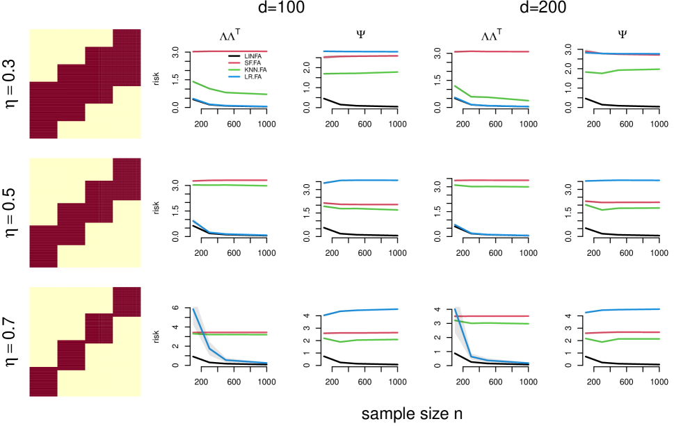
Figure 4: Covariance components estimation. The left panels illustrate the data observation pattern for three levels of missingness $\eta=0.3,0.5,0.7$ (Equation (4.1)), while the other panels display the risk for estimating the components $\Lambda\Lambda^{\mathrm{T}}$ and $\Psi$ for different number of variables $d$ and total sample size $n$.

4.2.2 Dimension reduction

In this simulation we assess the performance of LINFA and the alternative methods at predicting the latent factors. LINFA predicts the latent factors via Equation (2.4). Similarly, SF-FA, LR-FA, and KNN-FA, predict the latent factors via the equation $\hat{Z}_{r}=\hat{\Lambda}^{\mathrm{T}}\hat{\Sigma}^{-1}\tilde{X}_{r}$, where $\hat{\Lambda}$ and $\hat{\Sigma}$ are estimates from the the FA model fit on the completed data vectors $\tilde{X}_{1},\ldots,\tilde{X}_{n}\in\mathbb{R}^{d}$ in $\mathbf{X}_{\rm SF}$, $\mathbf{X}_{\rm KNN}$, and $\mathbf{X}_{\rm LR}$, respectively. We assess the precision of factor prediction using the trace $R^{2}$ metric of the regression of the estimated factors on the true ones [41, 17, 5], which is defined as

$$R^{2}(Z,\hat{Z})=\frac{{\rm tr}\left(Z^{\mathrm{T}}\hat{Z}(\hat{Z}^{\mathrm{T}}\hat{Z})^{-1}\hat{Z}^{\mathrm{T}}Z\right)}{{\rm tr}\left(Z^{\mathrm{T}}Z\right)},$$ (4.2)

where $Z\in\mathbb{R}^{n\times q}$ is the matrix containing the $n$ generated factor vectors $Z_{1},\ldots,Z_{n}$, and $\hat{Z}$ is the predicted counterpart. In Figure 5 we summarize the results of this simulation, showing that LINFA outperforms all other methods, although also LR-FA appears to perform well for small values of $\eta$.

4.2.3 Data completion

Let $V(r)=\{i\in V:X_{ri}~{}\text{is observed}\}$. Given the predicted factors $\hat{Z}_{r}$, LINFA can be used to predict the missing data entries $(X_{ri})_{i\notin V(r)}$ on the $r$-th sample by taking the corresponding entries of $\hat{X}_{r}$ in Equation (2.5). We compare the accuracy of LINFA at completing the data with the completions yielded in the data completion step in SF-FA, KNN-FA, and LR-FA. We compute the empirical (Pearson) correlation between the true unobserved values $(X_{ri})_{i\notin V(r)}$ and the predicted ones for all methods. We summarize the results in Figure 5, where we can see that LINFA outperforms all other methods, although LR-FA also yields satisfactory performance but only for small values of $\eta$.

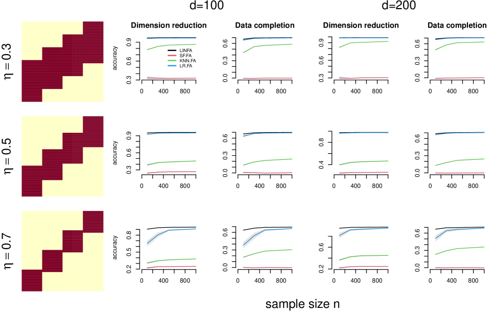
Figure 5: Dimension reduction and data completion. The left panels illustrate the data observation pattern for three levels of missingness $\eta=0.3,0.5,0.7$ (Equation (4.1)), while the other panels display the accuracy for dimension reduction and data completion for different number of variables $d$ and total sample size $n$.

4.2.4 Dependence structure recovery

In this simulation, we assess the accuracy of recovery of the dependence structure of the factor model. In our framework we may approach this task in two ways: (a) unconditionally on the factors by computing partial correlations $\rho_{ij}$ (Equation (2.6)) between variable pairs $(X_{ri},X_{rj})$, and (b) conditionally on the factors by computing the conditional correlations $\gamma_{ij}$ (Equation (2.8)) between observable variables and latent factors $(X_{ri},Z_{rj})$. Here, we focus on case (a). Figure 6 presents analogous results to Figure 3, but in terms of partial correlation estimation. Also in this case, LINFA outperforms all other methods.

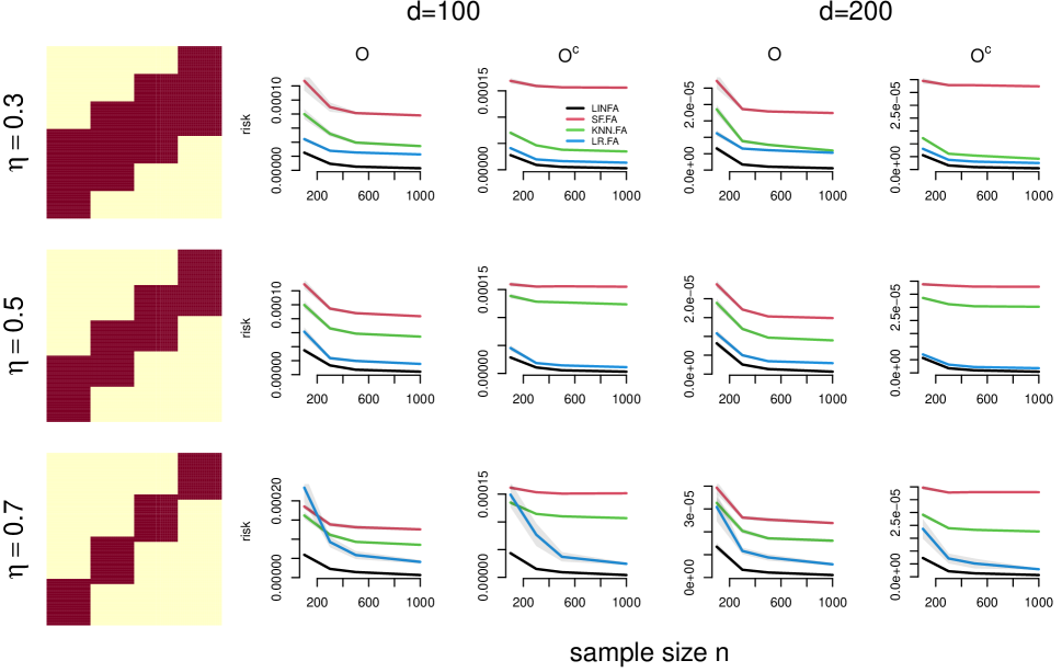
Figure 6: Partial correlation recovery. The left panels illustrate the data observation pattern for three levels of missingness $\eta=0.3,0.5,0.7$ (Equation (4.1)), while the other panels display the risk for partial correlation estimation in the set $O$ and $O^{c}$ for different number of variables $d$ and total sample size $n$.

4.2.5 Uncertainty quantification

In Figure 7 we compare the standard errors of Fisher transformed correlation MLEs obtained via LINFA approximated via parametric bootstrap (Algorithm 3) and nonparametric bootstrap (Algorithm 4) with the true ones approximated via Monte Carlo integration. Both methods appear to approximate the standard errors adequately although, as expected, the parametric bootstrap appears to perform better since the generative model and the one used in the bootstrap are in the same (Gaussian) family. In this simulation we used $d=100$ and $n=1000$, and $B=1000$ bootstrap samples for each method.

Figure 7: Uncertainty quantification. (A) True standard error of Fisher transformed MLE of correlations. (B) Parametric bootstrap approximations of the standard errors versus true standard errors. (C) Nonparametric bootstrap approximations of the standard errors versus true standard errors.

4.2.6 Model selection

In Figure 8 we display the boxplots of the selected number of factors $q_{\rm CV}$ and $q_{\rm AIC}$ obtained by minimizing $\textsc{Risk}_{\rm 2CV}$ (Equation (3.9)) and $\textsc{Risk}_{\rm AIC}$ (Equation (3.10)), respectively, versus the true value $q_{\rm true}=2,4,6,8,10$. The two criteria appear to yield similar selections and adequately recover the true number of factors under various settings with $K=3$, $d=50$, $n=500,1000$, $\eta=0.2,0.4$. However, AIC is less computationally expensive than cross-validation, so for large scale data sets it may be more convenient than cross-validation.

Figure 8: Model selection via 2-fold cross-validation and AIC. Boxplots of number of factors selected via 2-fold cross-validation ($q_{\rm CV}$) and AIC ($q_{\rm AIC}$) given true number of factors $q=2,4,6,8,10$, for $K=3$, $d=50$, and different proportions of missingness $\eta=0.2,0.4$ (Equation (4.1)) and total sample size $n=500,1000$.

5 Data analysis

We apply LINFA to the analysis of publicly available neuroscience data [43] consisting of calcium activity traces recorded from about 10,000 neurons in a 1mm $\times$ 1mm $\times$ 0.5mm volume of mouse visual cortex (70–385µm depth). The neuronal activities were simultaneously recorded in vivo via 2–photon imaging of GCaMP6s with 2.5Hz scan rate [31]. During the experiment, the animal was free to run on an air-floating ball in complete darkness for 105 minutes.

For our analyses, we focus on the most superficial layer of the brain portion containing 725 neurons. A graphical illustration of the neurons’ positions is in Figure 9A, where we depict four scenarios where we observe the full data ($\eta=0$; Equation (4.1)) or three subsets of the neurons over different sections of the recordings, inducing different proportions of missingness ($\eta=0.1,0.2,0.3$). In Figure 9B we show the corresponding observed data patterns which we create by appropriately obliterating portions of data. We estimate LINFA in each scenario with number of factors $q$ selected via AIC (Section 3.2). In Figure 9C we show partial correlation graphs (top 400 edges with largest $|\rho_{ij}|$, Equation (2.6)), and in parentheses we indicate the average square distance between correlations and partial correlations from the case of complete data ($\eta=0$). It appears that LINFA robustly recovers correlations and partial correlations for different levels of missingness. In Figure 9D we show the factor graphs (top 400 edges with largest $|\gamma_{ij}|$, Equation (2.8)), where the factor nodes (red squares) have positions computed as average neuron coordinates with weights proportional to the magnitudes of $\gamma_{ij}$’s. Specifically, if $Y\in\mathbb{R}^{d\times 2}$ contains the 2D coordinates of the $d$ neurons, then the position of the $j$-th factor is given by $(\sum_{i=1}^{d}Y_{i1}|\gamma_{ij}|/\sum_{i=1}^{d}|\gamma_{ij}|,~{}\sum_{i=1}^{d}Y_{i2}|\gamma_{ij}|/\sum_{i=1}^{d}|\gamma_{ij}|)$. It is interesting to note that the weighted positions of the most important factors (largest red squares; factors $j$ with largest $\sum_{i=1}^{d}|\gamma_{ij}|$) are approximately the same across different levels of missingness $\eta=0,0.1,0.2,0.3$.

Figure 9: (A) Observed sets of neurons simultaneously recorded ($V_{1}$ blue, $V_{2}$ red, and $V_{3}$ green) for different proportions of missingness $\eta=0,0.1,0.2,0.3$ (Equation (4.1)). (B) Illustration of corresponding observed data patterns. (C) Partial correlation graphs (top 400 edges), where in parenthesis we indicate the average square distance between correlations and partial correlations from the case of complete data ($\eta=0$). (D) Factor graphs (top 400 edges), where the factor nodes (red squares) have positions computed as average neuron coordinates with weights proportional to the relevant $\gamma_{ij}$’s (Equation (2.8)).

6 Discussion

In this paper we investigated the problem of estimating a factor model in case of structural or deterministic missingness, where the data vectors $X_{1},\ldots,X_{n}$ are not fully observed because of technological constraints, in which case several pairs of variables may even have no joint data observation. We proposed Linked Factor Analysis, or LINFA, a unified framework for covariance matrix completion, dimension reduction, data completion, and graphical dependence structure recovery in the case where the data suffer from structural missingness. We proposed an efficient Expectation-Maximization algorithm for the computation of the maximum likelihood estimator of the parameters of LINFA. This algorithm can be applied to data with arbitrary missingness patterns, and involves conditional expectations and updating equations all in closed form. Moreover, the maximization step of our proposed EM algorithm is accelerated by the Group Vertex Tessellation algorithm, which identifies a minimal partition of the vertex set to implement an efficient optimization in the maximization steps. We demonstrated the performance of LINFA in an extensive simulation study and with the analysis of neuroscience data. We expect LINFA to be useful for the multivariate analysis of data from disparate scientific fields where structural missingness is a common issue, such as genomics, psychology, and medicine, among many others.

Appendix A Start values of LINFA MLE EM Algorithm

We construct start values $(\Lambda_{0},\Psi_{0})$ for $(\Lambda,\Psi)$ of the LINFA MLE Algorithm 2 as follows. We first complete the observed data by filling any missing data point about node $j$ with the simple average of all observed values about node $j$. This yields a $n\times d$ data matrix $\tilde{\mathbf{X}}$. We then obtain the sample covariance matrix $\tilde{\Sigma}$ and its spectral decomposition

$$\tilde{\Sigma}=V\Phi V^{T}$$ (A.1)

where $V\in\mathbb{R}^{d\times d}$ contains the eigenvectors and $\Phi$ is the diagonal matrix containing eigenvalues. The unrotated start value for $\Lambda$ is then defined as

$$\tilde{\Lambda}_{0}~{}=~{}V_{.,1:q}\Phi_{1:q,1:q}^{1/2}$$ (A.2)

where $V_{.,1:q}$ contains the first $q$ columns of $V$ and $\Phi_{1:q,1:q}^{1/2}={\rm diag}(\sqrt{\Phi_{11}},...,\sqrt{\Phi_{qq}})$. The start value for $\Psi$ is defined as

$$\Psi_{0}~{}=~{}{\rm Diag}(\tilde{\Sigma})$$

Finally, we compute the matrix $R$ of eigenvectors of $\frac{1}{d}\tilde{\Lambda}_{0}^{\mathrm{T}}\Psi_{0}^{-1}\tilde{\Lambda}_{0}$ to obtain the rotated start value

$$\Lambda_{0}=\tilde{\Lambda}_{0}R$$

References

- Ahn and Horenstein, [2013] Ahn, S. C. and Horenstein, A. R. (2013). Eigenvalue ratio test for the number of factors. Econometrica, 81(3):1203–1227.
- Akaike, [1974] Akaike, H. (1974). A new look at the statistical model identification. IEEE transactions on automatic control, 19(6):716–723.
- Anderson and Rubin, [1956] Anderson, T. W. and Rubin, H. (1956). Statistical inference in factor analysis. In Proceedings of the third Berkeley symposium on mathematical statistics and probability, volume 5, pages 111–150.
- Bai and Li, [2012] Bai, J. and Li, K. (2012). Statistical analysis of factor models of high dimension. The Annals of Statistics, 40(1):436–465.
- Bańbura and Modugno, [2014] Bańbura, M. and Modugno, M. (2014). Maximum likelihood estimation of factor models on datasets with arbitrary pattern of missing data. Journal of applied econometrics, 29(1):133–160.
- Barratt, [1965] Barratt, E. S. (1965). Factor analysis of some psychometric measures of impulsiveness and anxiety. Psychological reports, 16(2):547–554.
- Bhattacharya and Dunson, [2011] Bhattacharya, A. and Dunson, D. B. (2011). Sparse bayesian infinite factor models. Biometrika, pages 291–306.
- Bishop and Byron, [2014] Bishop, W. E. and Byron, M. Y. (2014). Deterministic symmetric positive semidefinite matrix completion. In Advances in Neural Information Processing Systems, pages 2762–2770.
- Bong et al., [2020] Bong, H., Liu, Z., Ren, Z., Smith, M., Ventura, V., and Robert, K. E. (2020). Latent dynamic factor analysis of high-dimensional neural recordings. Advances in neural information processing systems, 33.
- Campbell, [1996] Campbell, J. Y. (1996). Understanding risk and return. Journal of Political economy, 104(2):298–345.
- Candès and Plan, [2010] Candès, E. J. and Plan, Y. (2010). Matrix completion with noise. Proceedings of the IEEE, 98(6):925–936.
- Candès and Recht, [2009] Candès, E. J. and Recht, B. (2009). Exact matrix completion via convex optimization. Foundations of Computational mathematics, 9(6):717.
- Caner and Han, [2014] Caner, M. and Han, X. (2014). Selecting the correct number of factors in approximate factor models: The large panel case with group bridge estimators. Journal of Business & Economic Statistics, 32(3):359–374.
- Carvalho et al., [2008] Carvalho, C. M., Chang, J., Lucas, J. E., Nevins, J. R., Wang, Q., and West, M. (2008). High-dimensional sparse factor modeling: applications in gene expression genomics. Journal of the American Statistical Association, 103(484):1438–1456.
- Chamberlain and Rothschild, [1982] Chamberlain, G. and Rothschild, M. (1982). Arbitrage, factor structure, and mean-variance analysis on large asset markets.
- Dempster et al., [1977] Dempster, A. P., Laird, N. M., and Rubin, D. B. (1977). Maximum likelihood from incomplete data via the em algorithm. Journal of the Royal Statistical Society: Series B (Methodological), 39(1):1–22.
- Doz et al., [2012] Doz, C., Giannone, D., and Reichlin, L. (2012). A quasi–maximum likelihood approach for large, approximate dynamic factor models. Review of economics and statistics, 94(4):1014–1024.
- Fama and French, [1992] Fama, E. F. and French, K. R. (1992). The cross-section of expected stock returns. the Journal of Finance, 47(2):427–465.
- Freeman and Grajski, [1987] Freeman, W. J. and Grajski, K. A. (1987). Relation of olfactory eeg to behavior: factor analysis. Behavioral neuroscience, 101(6):766.
- Haslbeck and van Bork, [2022] Haslbeck, J. and van Bork, R. (2022). Estimating the number of factors in exploratory factor analysis via out-of-sample prediction errors. Psychological Methods.
- James et al., [2021] James, G., Witten, D., Hastie, T., and Tibshirani, R. (2021). An introduction to statistical learning, second edition. New York: Springers.
- Jennrich, [1974] Jennrich, R. I. (1974). Simplified formulae for standard errors in maximum-likelihood factor analysis. British Journal of Mathematical and Statistical Psychology, 27(1):122–131.
- Kneip and Sarda, [2011] Kneip, A. and Sarda, P. (2011). Factor models and variable selection in high-dimensional regression analysis. The Annals of Statistics, 39(5):2410–2447.
- Knowles and Ghahramani, [2011] Knowles, D. and Ghahramani, Z. (2011). Nonparametric bayesian sparse factor models with application to gene expression modeling. The Annals of Applied Statistics, 5(2B):1534–1552.
- Kolar and Xing, [2012] Kolar, M. and Xing, E. P. (2012). Estimating sparse precision matrices from data with missing values. In International Conference on Machine Learning, pages 635–642.
- Kurtz et al., [2000] Kurtz, M. J., Eichhorn, G., Accomazzi, A., Grant, C. S., Murray, S. S., and Watson, J. M. (2000). The nasa astrophysics data system: Overview. Astronomy and astrophysics supplement series, 143(1):41–59.
- Lawley and Maxwell, [1962] Lawley, D. N. and Maxwell, A. E. (1962). Factor analysis as a statistical method. Journal of the Royal Statistical Society. Series D (The Statistician), 12(3):209–229.
- Loh and Wainwright, [2011] Loh, P.-L. and Wainwright, M. J. (2011). High-dimensional regression with noisy and missing data: Provable guarantees with non-convexity. In Advances in Neural Information Processing Systems, pages 2726–2734.
- Mazumder et al., [2010] Mazumder, R., Hastie, T., and Tibshirani, R. (2010). Spectral regularization algorithms for learning large incomplete matrices. The Journal of Machine Learning Research, 11:2287–2322.
- Onatski, [2009] Onatski, A. (2009). Testing hypotheses about the number of factors in large factor models. Econometrica, 77(5):1447–1479.
- Pachitariu et al., [2017] Pachitariu, M., Stringer, C., Dipoppa, M., Schröder, S., Rossi, L. F., Dalgleish, H., Carandini, M., and Harris, K. D. (2017). Suite2p: beyond 10,000 neurons with standard two-photon microscopy. Biorxiv, page 061507.
- Patat et al., [1994] Patat, F., Barbon, R., Cappellaro, E., and Turatto, M. (1994). Light curves of type ii supernovae. 2: The analysis. Astronomy and Astrophysics, 282:731–741.
- Preacher et al., [2013] Preacher, K. J., Zhang, G., Kim, C., and Mels, G. (2013). Choosing the optimal number of factors in exploratory factor analysis: A model selection perspective. Multivariate behavioral research, 48(1):28–56.
- Rao, [1955] Rao, C. R. (1955). Estimation and tests of significance in factor analysis. Psychometrika, 20(2):93–111.
- Ročková and George, [2016] Ročková, V. and George, E. I. (2016). Fast bayesian factor analysis via automatic rotations to sparsity. Journal of the American Statistical Association, 111(516):1608–1622.
- Russell, [2002] Russell, D. W. (2002). In search of underlying dimensions: The use (and abuse) of factor analysis in personality and social psychology bulletin. Personality and social psychology bulletin, 28(12):1629–1646.
- Shumway and Stoffer, [1982] Shumway, R. H. and Stoffer, D. S. (1982). An approach to time series smoothing and forecasting using the em algorithm. Journal of time series analysis, 3(4):253–264.
- Soudry et al., [2015] Soudry, D., Keshri, S., Stinson, P., Oh, M.-h., Iyengar, G., and Paninski, L. (2015). Efficient “shotgun” inference of neural connectivity from highly sub-sampled activity data. PLoS computational biology, 11(10):e1004464.
- Srivastava et al., [2017] Srivastava, S., Engelhardt, B. E., and Dunson, D. B. (2017). Expandable factor analysis. Biometrika, 104(3):649–663.
- Städler and Bühlmann, [2012] Städler, N. and Bühlmann, P. (2012). Missing values: sparse inverse covariance estimation and an extension to sparse regression. Statistics and Computing, 22(1):219–235.
- [41] Stock, J. H. and Watson, M. W. (2002a). Forecasting using principal components from a large number of predictors. Journal of the American statistical association, 97(460):1167–1179.
- [42] Stock, J. H. and Watson, M. W. (2002b). Macroeconomic forecasting using diffusion indexes. Journal of Business & Economic Statistics, 20(2):147–162.
- Stringer et al., [2019] Stringer, C., Pachitariu, M., Steinmetz, N., Reddy, C. B., Carandini, M., and Harris, K. D. (2019). Spontaneous behaviors drive multidimensional, brainwide activity. Science, 364(6437):eaav7893.
- Tsai and Tsay, [2010] Tsai, H. and Tsay, R. S. (2010). Constrained factor models. Journal of the American Statistical Association, 105(492):1593–1605.
- Vinci, [2024] Vinci, G. (2024). Unsupervised learning, chapter 12 in statistical methods in epilepsy. Routhledge.
- Vinci et al., [2019] Vinci, G., Dasarathy, G., and Allen, G. I. (2019). Graph quilting: graphical model selection from partially observed covariances. arXiv preprint arXiv:1912.05573.
- Vinci et al., [2018] Vinci, G., Ventura, V., Smith, M., and Kass, R. E. (2018). Adjusted regularization in latent graphical models: Application to multiple-neuron spike count data. The Annals of Applied Statistics, 12(2):1068–1095.
- Watson and Engle, [1983] Watson, M. W. and Engle, R. F. (1983). Alternative algorithms for the estimation of dynamic factor, mimic and varying coefficient regression models. Journal of Econometrics, 23(3):385–400.
- Zhang, [2014] Zhang, G. (2014). Estimating standard errors in exploratory factor analysis. Multivariate behavioral research, 49(4):339–353.