Hashing Modulo Context-Sensitive $\alpha$-Equivalence

Abstract.

The notion of $\alpha$-equivalence between $\lambda$-terms is commonly used to identify terms that are considered equal. However, due to the primitive treatment of free variables, this notion falls short when comparing subterms occurring within a larger context. Depending on the usage of the Barendregt convention (choosing different variable names for all involved binders), it will equate either too few or too many subterms. We introduce a formal notion of context-sensitive $\alpha$-equivalence, where two open terms can be compared within a context that resolves their free variables. We show that this equivalence coincides exactly with the notion of bisimulation equivalence. Furthermore, we present an efficient $O(n\log n)$ runtime algorithm that identifies $\lambda$-terms modulo context-sensitive $\alpha$-equivalence, improving upon a previously established $O(n\log^{2}n)$ bound for a hashing modulo ordinary $\alpha$-equivalence by Maziarz et al (DBLP:conf/pldi/MaziarzELFJ21, ). Hashing $\lambda$-terms is useful in many applications that require common subterm elimination and structure sharing. We employ the algorithm to obtain a large-scale, densely packed, interconnected graph of mathematical knowledge from the Coq proof assistant for machine learning purposes.

1. Introduction

This paper studies equivalence of $\lambda$-terms modulo renaming of bound variables, so called $\alpha$-equivalence. This has been studied extensively in the history of $\lambda$-calculus, starting with Church (Church, ). The overview book by Barendregt (BarendregtLambdaCalc, ) also defines and studies it in detail. There, $\alpha$-equivalence is defined as a relation $t=_{\alpha}u$ between two $\lambda$-terms that captures the idea that $t$ can be obtained from $u$ by renaming bound variables.

In the present paper we study a more general situation where $t$ and $u$ are accompanied by a context that binds their free variables. Hence, we study the notion of context-sensitive $\alpha$-equivalence, which we will show to coincide with bisimulation when interpreting $\lambda$-terms as a graph. This notion has particular importance in case one wants to semantically compare and de-duplicate the subterms of huge $\lambda$-terms (e.g. a dataset extracted from the Coq proof assistant (the_coq_development_team_2020_4021912, )). To this end, we also define an efficient $O(n\log n)$-time hashing algorithm that respects this equivalence, in the sense that sub-terms receive the same hash if and only if they are context-sensitive $\alpha$-equivalent.

1.1. Problem Description

The $\alpha$-equivalence relation equates $\lambda$-terms modulo the names of binders. For example, $\lambda x.\lambda y.x=_{\alpha}\lambda y.\lambda x.y$. De Bruijn indices are a way to make the syntax of $\lambda$-terms invariant w.r.t. the $\alpha$-equivalence relation. Using de Bruijn indices, both terms above would be represented by $\lambda\lambda\ \underline{1}$, and would hence be syntactically equal.

The $\alpha$-equivalence relation becomes less clear when free variables are involved. Usually, it is understood that terms are only equal when all occurrences of free variables are equal. However, the situation is more complicated when considering free variables within a known context. Consider the example

(0.1) $$\lambda t.\ Q\ (\lambda p.\lambda f.\ f\ t)\ (\lambda g.\ g\ t).$$

In this term, are the subterms $\lambda f.\ f\ t$ and $\lambda g.\ g\ t$ considered $\alpha$-equivalent? Most would agree they are equivalent because we can share these terms with a let-construct without changing the meaning of the term:

(0.2) $$\lambda t.\ \text{let}\ s\coloneqq\lambda f.\ f\ t\text{ in }Q\ (\lambda p.s)\ s$$

Here, the justification that we are “not changing the meaning of the term” is that one $\beta$-reduction of the introduced let will give us the original term (modulo renaming of bound variables). However, when we represent the original term with de Bruijn indices, these two sub-terms are not syntactically equal.

$$\lambda\ Q\ (\lambda\lambda\ \underline{0}\ \underline{2})\ (\lambda\ \underline{0}\ \underline{1})$$

The promise of de Bruijn indices has failed us! If we want to find the common sub-terms of a program, we cannot simply convert the program to use de Bruijn indices, hash the program into a Merkle tree, and call it a day.

In addition to false negatives, de Bruijn indices can also lead to false positives. Consider the example

(0.3) $$\lambda t.\ Q\ (\lambda p.\lambda f.\ f\ p)\ (\lambda g.\ g\ t).$$

Here, the subterms $\lambda f.\ f\ p$ and $\lambda g.\ g\ t$ are not $\alpha$-equivalent. However, when expressed using de Bruijn indices they become equal.

$$\lambda\ Q\ (\lambda\lambda\ \underline{0}\ \underline{1})\ (\lambda\ \underline{0}\ \underline{1})$$

Given these counter-examples, one might conclude that de Bruijn indices are not as useful in deciding equality between (sub)-terms as is commonly thought. Unfortunately, the situation is not much better for $\lambda$-terms with ordinary named variables. Take for example this naive attempt at defining context-sensitive $\alpha$-equivalence:

Two subterms of $t$ are $\alpha$-equivalent in the context of $t$ if the bound variables in $t$ can be renamed such that the subterms become syntactically equal.

An immediate counter-example to this definition is the term $Q\ (\lambda x.x)\ (\lambda xy.\ x)$ and the question wether the two occurrences of the variable $x$ are $\alpha$-equivalent. According to the definition, yes, but the variables correspond to binders that cannot possibly be considered equivalent.

At this point, it is not even clear what precise equivalence relation we are looking for, even though many people would “know an equivalence between subterms when they see one.” The only intuitive idea we have to build on is the introduction of a let-abstraction in Formula 0.2. But, as we will see, this is not sufficient on its own.

1.2. Fork Equivalence

Let us return to Example 0.1, where we used let-abstraction to “show” that two subterms are equal. We make this slightly more precise (a fully formal treatment can be found in Section 2). To conveniently talk about the equality of subterms within a context, we underline the two terms of interest. This allows us to restate the question in Example 0.1 as follows.

(0.4) $$\begin{gathered}\lambda t.\ Q\ (\lambda p.\underline{\lambda f.\ f\ t})\ (\underline{\lambda g.\ g\ t})\\ \lambda\ Q\ (\lambda\underline{\lambda\ \underline{0}\ \underline{2}})\ (\underline{\lambda\ \underline{0}\ \underline{1}})\end{gathered}$$

The underlined subterms are the subject of the context-sensitive $\alpha$-equivalence. The remainder of the term, which we can write as $\lambda t.\ Q\ (\lambda p.\ \_)\ \_$ or $\lambda\ Q\ (\lambda\ \_)\ \_$, is the context in which the equivalence is to be shown. Now, in order to perform the let-abstraction, we must split the context into two pieces, such that we can insert the let in between. In this case, the split we make is $\lambda t.\ \_$ and $Q\ (\lambda p.\ \_)\ \_$. We can then show that the term $\lambda f.\ f\ t$ is closed under the outer context and when we substitute it into the holes in the inner context (while avoiding variable capture), we obtain the original term. Hence, we can reassemble everything to obtain the same term from Example 0.2.

$$\lambda t.\ \text{let}\ s\coloneqq\lambda f.\ f\ t\text{ in }Q\ (\lambda p.s)\ s$$

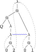
(a) The single fork in Example 0.4.

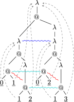
(b) Illustration of sub-forks and transitivity from Example 0.5.

Figure 1. Illustrations of forks in terms built from de Bruijn indices. Subject terms are related through a squiggly line. Back-edges from variables to binders are illustrative only.

Let-abstractable subterms are the first ingredient of the fork-equivalence relation. This relation is named so because the relation is built upon a fork, starting with a single outer context that forms the base of the fork. Then follows an inner context that acts as the bifurcation of the base towards the two subjects. The fork is shown in Figure 1(a).

However, the definition of fork equivalence is not complete. Let-abstraction only allows us to compare subjects that share a common context. However, when two subjects are closed, their context is irrelevant. In that situation, both subjects may occur in a completely different context while still being equivalent. This gives rise to an equivalence relation $\sim_{\text{f}}$ formed between two pairs of a subject and context. This allows establishing equivalences between closed subjects such as

$$P\ (\underline{\lambda x.x})\sim_{\text{f}}Q\ (\underline{\lambda y.y}).$$

In general, in addition to let-abstraction, we say that a fork can also be established between any two closed subjects that are equal modulo variable renaming (or syntactically equal in the case of de Bruijn indices). Closed subjects can be accompanied by arbitrary contexts, as they can never influence the meaning of the subjects. Let-abstraction, when phrased as a relation $\sim_{\text{f}}$, would still require a common context even though that common context is stated twice. Our running Example 0.4 would be phrased as

$$\lambda t.\ Q\ (\lambda p.\underline{\lambda f.\ f\ t})\ (\lambda g.\ g\ t)\sim_{\text{f}}\lambda t.\ Q\ (\lambda p.\lambda f.\ f\ t)\ (\underline{\lambda g.\ g\ t}).$$

To complete the definition of fork equivalence, we must also extend it with both the sub-fork and with transitivity of forks. The following example illustrates the need for these extensions:

(0.5) $$\lambda t.\ (\lambda x.\ \underline{x\ t}\ (\lambda y.\ x\ t))\ (\lambda z.\ \lambda x.\ x\ t\ (\lambda y.\ x\ t))$$

$$\sim_{\text{f}}{} \lambda t.\ (\lambda x.\ x\ t\ (\lambda y.\ \underline{x\ t}))\ (\lambda z.\ \lambda x.\ x\ t\ (\lambda y.\ x\ t))$$

$$\sim_{\text{f}}{} \lambda t.\ (\lambda x.\ x\ t\ (\lambda y.\ x\ t))\ (\lambda z.\ \lambda x.\ x\ t\ (\lambda y.\ \underline{x\ t}))$$

Notice how the first equivalence can be established because the subjects are let-abstractable. For the second equivalence, we have no such luck. There is no place where we could split the context such that both instances of $x\ t$ would be closed under the outer context. Note, however, that if we widen the subject $x\ t$ to $\lambda x.\ x\ t\ (\lambda y.\ x\ t)$, a let-abstraction can indeed be performed. Because both underscored instances of $x\ t$ occur in the same position in this wider term, we allow for the creation of a sub-fork between them. Finally, to demonstrate the transitivity concept, we can combine both let-abstractions in the following term, such that all underscored locations coincide:

$$\lambda t.\ \text{let }u\coloneqq(\lambda x.\ \text{let }v\coloneqq x\ t\text{ in }v\ \lambda y.v)\text{ in }u\ \lambda z.u$$

This is further illustrated in Figure 1(b). The two red forks are created by let-abstraction, as well as the dark blue fork. The two teal lines are sub-forks of the dark blue fork. Finally, using transitivity, fork equivalence is formed between all four connected sub-terms.

At this point, the definition of fork equivalence includes (1) let-abstraction, (2) equivalence between equal closed terms, (3) the sub-fork and (4) a transitive closure. It is not obvious that this relation is indeed sound and complete w.r.t. the intuitive notion of equivalence between subterms. To mitigate such doubts, we will now introduce a completely separate equivalence relation that will be shown equal to fork equivalence in Appendix A.

1.3. Equivalence through Bisimulation

For our second equivalence relation, we will interpret $\lambda$-terms as directed graphs. The skeleton of the graph is formed by the abstract syntax tree of the $\lambda$-term, but instead of having variables or de Bruijn indices in the leaves, they have a pointer back to the location where the variable was bound.

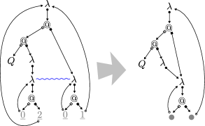
(a) Subterms of Example 0.1 are bisimilar. Their nodes can be merged, resulting in variables without a unique de Bruijn index.

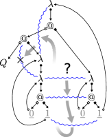
(b) Subterms of Example 0.3 are not bisimilar, shown by a counter-example.

Figure 2. Illustrations of $\lambda$-terms as unordered graphs with labeled edges. Subject terms are related through a squiggly line. De Bruijn indices in variables are for illustrative purposes only.

With such an interpretation, it becomes possible to define context-sensitive $\alpha$-equivalence as the well-known notion of the bisimilarity relation that is common in the analysis of labeled transition systems and many other (potentially) infinite structures (DBLP:books/daglib/0020348, ). As a refresher, we will restate the definition of bisimilarity on a directed graph with labeled nodes and edges: A relation $R$ between nodes is a bisimulation relation when for all nodes $(p_{1},p_{2})\in R$ the labels of $p_{1}$ and $p_{2}$ are equal and

$$\begin{split}&\text{if}\ p_{1}\xrightarrow{a}q_{1}\ \text{then there exists}\ q_{2}\ \text{such that}\ p_{2}\xrightarrow{a}q_{2}\ \text{and}\ (q_{1},q_{2})\in R\\ &\text{if}\ p_{2}\xrightarrow{a}q_{2}\ \text{then there exists}\ q_{1}\ \text{such that}\ p_{1}\xrightarrow{a}q_{1}\ \text{and}\ (q_{1},q_{2})\in R.\end{split}$$

Two nodes $p_{1}$ and $p_{2}$ in a graph are then considered bisimilar if there exists a bisimulation relation $R$ such that $(p_{1},p_{2})\in R$. The bisimilarity relation is the union of all bisimulation relations, and is itself a bisimulation.

Figure 2(a) shows the term in Example 0.1 as a graph. Due to the unordered nature of graphs, in contrast to more common presentation of syntax trees as ordered trees, edges are annotated with a shape that represents their label. It is straight-forward to build a relation $R$ that includes the two subject terms and satisfies the requirements of a bisimulation relation. The existence of the bisimulation certifies that we can de-duplicate the two subject terms in the graph structure without changing their meaning. Note that as a result, variables can no longer be assigned a unique de Bruijn index.

Figure 2(b) shows how the subterms in Example 0.3 are not bisimilar. This is done by assuming a valid bisimulation relation $R$ that contains the two subject terms. One can then simultaneously follow equal edges on both sides until two nodes with different labels are encountered that are not allowed to be in $R$.

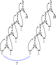
Figure 3. To decide wether two variables are bisimilar, we must examine bisimilarity between far-away terms $A$ and $B$.

Deciding wether two subterms are equal is not always as easy as the illustrations in Figure 2 suggest. Consider the bisimulation question in Figure 3 between two variables. To decide wether the variables are bisimilar, we must repeatedly travel up and down into the term jumping between variables and their binders, until we reach the root. From there, we must travel into the subterms $A$ and $B$. The two variables will be bisimilar if and only if $A$ and $B$ are bisimilar. This shows that no matter the size of the subject terms, one might need to traverse and examine the entire context in order to decide their bisimilarity. A decision procedure or hashing scheme must take all of this information into account while still being efficient.

Finally, we note the importance of having variable nodes in the embedding of $\lambda$-terms as graphs. Since variable nodes only have a single incoming edge and a single outgoing back-edge to the corresponding binder, one might be tempted to skip the variable node altogether. However, such an embedding would lead to a situation where we share too many terms. One example of such problems is the following sequence of terms that should not be bisimilar.

$$\lambda x.x\sim_{\text{b}}\lambda y.\lambda x.x\sim_{\text{b}}\lambda z.\lambda y.\lambda x.x\sim_{\text{b}}\ldots$$

However, under the following encoding, which omits variables, these terms would be bisimilar.

For some readers, it might be obvious that the bisimilarity relation indeed corresponds to the intuitive notion of subterm equality, while for others this might be less clear. We hope that by providing both the notion of fork equivalence an bisimilarity, and proving they are equal in Appendix A, the reader will be convinced that this is indeed the intuitively expected relation.

With the relation between $\lambda$-terms and labeled transition systems established, we can now borrow from the wealth of research into process algebras to find an algorithm that constructs the full context-sensitive $\alpha$-equivalence of $\lambda$-terms. Indeed, we can use an off-the-shelf bisimulation decision procedure to solve our problem in $O(n\log n)$ time (DBLP:journals/tcs/DovierPP04, ).

Such an off-the-shelf algorithm is not fully satisfactory however. One reason is that the class of graphs induced by $\lambda$-terms is a significant restriction that allows for the creation of a simpler algorithm. In particular, we will construct a simple recursive algorithm that only relies on well-known operations in $\lambda$-calculus, such as capture-avoiding substitution. Another reason to avoid an off-the-shelf algorithm is that we would like to assign a uniquely identifying hash to each subterm for quick comparisons. We are not aware of existing graph-hashing algorithms that operate modulo bisimilarity. In Section 3 we present hashing algorithms for $\lambda$-terms that respects the context-sensitive $\alpha$-equivalence relation.

1.4. Context-Sensitive $\alpha$-Equivalence versus Ordinary $\alpha$-Equivalence

We will now explore some of the differences between context-sensitive $\alpha$-equivalence and ordinary $\alpha$-equivalence. Previously, Maziarz et al (DBLP:conf/pldi/MaziarzELFJ21, ) have constructed a hashing scheme modulo ordinary $\alpha$-equivalence. How does this differ from our scheme and when is one relation or algorithm to be preferred over another?

To examine this question, we again look at the term in Example 0.5 as visualized in Figure 1(b).

$$\lambda t.\ (\lambda x.\ x\ t\ (\lambda y.\ x\ t))\ (\lambda z.\ \lambda x.\ x\ t\ (\lambda y.\ x\ t))$$

$$\lambda t.\ (\lambda x.\ \underline{0}\ \underline{1}\ (\lambda y.\ \underline{1}\ \underline{2}))\ (\lambda z.\ \lambda x.\ \underline{0}\ \underline{2}\ (\lambda y.\ \underline{1}\ \underline{3}))$$

This term contains four instances of the term $x\ t$, all of whom are represented differently using de Bruijn indices, and all of whom are considered equal modulo context-sensitive $\alpha$-equivalence. Which of these instances of $x\ t$ are equal under ordinary $\alpha$-equivalence? This is a tricky question to answer. Both the variables $x$ and $t$ are free in the term $(x\ t)$. As such, under ordinary $\alpha$-equivalence, they would be compared syntactically. This would indeed make all four instances $\alpha$-equivalent. However, such an interpretation would get us into trouble when we rename the bound variables in the term. This may change the variable names in the subterms, which in turn may cause them to no longer be $\alpha$-equivalent. Hence, $\alpha$-equality between subterms is contingent on the particular choice of bound variable names we have made. That is not acceptable. Maziarz et al. solve this ambiguity by globally enforcing the Barendregt convention on the entire universe of $\lambda$-terms. That is, no two binders may ever have the same name. The term in our example does not satisfy the Barendregt convention. We must rewrite it to

$$\lambda t.\ (\lambda x_{1}.\ x_{1}\ t\ (\lambda y_{1}.\ x_{1}\ t))\ (\lambda z.\ \lambda x_{2}.\ x_{2}\ t\ (\lambda y_{2}.\ x_{2}\ t)).$$

We now have two $\alpha$-equivalent instances of $x_{1}\ t$ and two $\alpha$-equivalent instances of $x_{2}\ t$. This is contrasted by context-sensitive $\alpha$-equivalence, where all four terms are equal. In general, we have that ordinary $\alpha$-equivalence is a sub-relation of context-sensitive $\alpha$-equivalence. This can lead to some counter-intuitive situations: The subterms $\lambda x_{1}.\ x_{1}\ t\ (\lambda y_{1}.\ x_{1}\ t)$ and $\lambda x_{2}.\ x_{2}\ t\ (\lambda y_{2}.\ x_{2}\ t)$ are considered $\alpha$-equivalent according to Maziarz et al., but not all their constituent parts are mutually $\alpha$-equivalent. No such issues exist for the context-sensitive variant.

Trade-offs between the two relations are as follows:

• Ordinary $\alpha$-equivalence is simple. It is defined on $\lambda$-terms, while context-sensitive $\alpha$-equivalence needs an additional context.

• Ordinary $\alpha$-equivalence cannot be defined properly on open terms encoded with de Bruijn indices. Syntactic comparisons between open de Bruijn indices leads to incorrect results (see Example 0.3). A hybrid approach, such as a locally-nameless representation (DBLP:journals/jar/Chargueraud12, ), is required to resolve this. Context-sensitive $\alpha$-equivalence can be properly defined for any representation of $\lambda$-terms.

• When interpreting $\lambda$-terms as a graph, one should use context-sensitive $\alpha$-equivalence because it equals the graph-theoretic notion of bisimilarity.

• For tasks like common subterm elimination in compilers, both relations may be appropriate because there one usually seeks to find the largest $\alpha$-equivalent subterms and not their descendants. Both relations achieve this.

Furthermore, the trade-offs between the hashing algorithm in this paper and the one by Maziarz et al. are as follows:

• Our algorithm hashes all nodes in a term in $O(n\log n)$ time while Maziarz et al. require $O(n\log^{2}n)$ time.

• Maziarz et al. require a global preprocessing step to enforce the Barendregt convention. No such step is required for our algorithm.

• The algorithm by Maziarz et al. is compositional. That is, given two hashed terms $t$ and $u$, one can relatively efficiently compute the hash for $(t\ u)$. This may be a desirable property in a compiler, allowing one to maintain a correct hashes while rewriting a terms during optimization passes. Compositionality is not possible for context-sensitive $\alpha$-equivalence, because changing the context may require a change in the hash of all subterms (see Figure 3).

• Maziarz et al. rely fundamentally on named variables, while we rely fundamentally on de Bruijn indices. In both cases, it is possible to do a representation conversion before hashing, but both algorithms have a clear “native” representation. Much has been said around the relative merits of $\lambda$-term representations (DBLP:journals/entcs/BerghoferU07, ), and we do not wish to make a value judgement here. It is good to know there are viable algorithms for both representational approaches, even if those algorithms have subtle differences in how they operate.

1.5. Applications

The original motivation for the subterm sharing algorithm in this paper was the creation of a large-scale, graph-based machine learning dataset of terms in the calculus of inductive constructions, exported from the Coq Proof Assistant (the_coq_development_team_2020_4021912, ). Extracting data from over a hundred Coq developments leads to a single, interconnected graph containing over 520k definitions, theorems and proofs. For each node in this graph we calculate a hash modulo context-sensitive $\alpha$-equivalence. The hash is then used to maximally share all subterms, resulting in a dense graph with approximately 250 million nodes. A very small section of this graph is visualized in Figure 4. More details on the construction can be found elsewhere (web-paper, ). Experiments show that subterm sharing allows for an 88% reduction in the number of nodes. Hence, without sharing, such a graph would have over 2 billion nodes. Identifying identical subterms in a graph is helpful semantic information that can be used by machine learning algorithms to make predictions. The graph dataset has been leveraged to train a state of the art graph neural network to synthesize proofs in Coq (graph2tac, ).

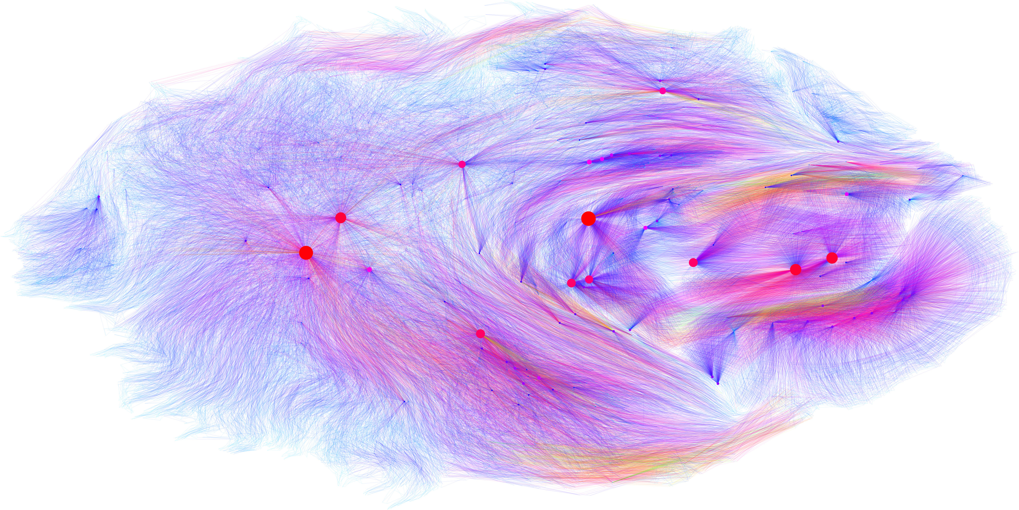
Figure 4. A visualization of a maximally shared graph of CIC terms extracted from Coq’s Prelude.

In addition to our original motivation, we expect our algorithm to be useful in other applications as well. In compilers, common sub-expression elimination is a common optimization pass (DBLP:conf/comop/Cocke70, ) that can be performed quickly using our algorithm. This was the original motivation for the algorithm by Maziarz et al. (DBLP:conf/pldi/MaziarzELFJ21, ). Similarly, the identity hashes of subterms may be used to build indexes of program libraries that can then be queried to find opportunities for code sharing (DBLP:conf/iwsc/ThomsenH12, ) or plagiarism detection (DBLP:conf/bwcca/ZhaoXFC15, ).

1.6. Contributions

In this paper, we develop a notion of context-sensitive $\alpha$-equivalence that compares potentially open terms within a context. We define this notion both through let-abstraction and bisimulation. Even though these notions seem quite dissimilar, we prove them to be equivalent. We present an efficient decision procedure and hashing algorithm that identifies terms modulo context-sensitive $\alpha$-equivalence. These algorithms have been successfully used to efficiently encode a graph of Coq terms for machine learning purposes. A reference implementation written in OCaml is available (lasse_blaauwbroek_2023_10421517, ).

The remainder of the paper is organized as follows. Section 2 first introduces the preliminaries followed by the formal definitions of forking equivalence in Section 2.4 and bisimilarity in Section 2.5. Then, Section 3.1 presents a simple, naive algorithm for hashing $\lambda$-terms in $O(n^{2})$ time. This is then refined in Section 3.2 and finally a concrete, $O(n\log n)$ hashing algorithm implemented in OCaml is presented in Section 3.3. Proofs of equality between the two relations and the algorithms can be found in Appendix A.

2. Definitions

In this section, we will further formalize the equivalence relations presented in the introduction. From this point, we will only consider $\lambda$-terms encoded with de Bruijn indices. The algorithms rely heavily on the fact that two $\alpha$-equivalent closed terms encoded using de Bruijn indices are syntactically equal. That said, the equivalence relations and the proofs of equality between them also work when one uses $\lambda$-terms with named variables modulo ordinary $\alpha$-equivalence. For the sake of legibility, we will frequently still give examples using $\lambda$-terms with named variables.

2.1. Terms, Positions and Indexing

Definition 2.0 ($\lambda$-terms).

$\lambda$-terms with de Bruijn indices are generated by the grammar

$$t\Coloneqq\underline{i}\mid t\ t\mid\lambda\ t,$$

where a de Bruijn index $\underline{i}$ is a nonnegative integer. We denote $t[\underline{i}\coloneqq u]$ to be the capture-avoiding substitution of variable $\underline{i}$ by $u$ in $t$. Furthermore, let $\sigma=[u_{0},u_{1},\ldots,u_{n-1}]$ be a list of terms. Then $t\sigma$ denotes the simultaneous subtitution of all variables $\underline{i}$ by $u_{i}$ in $t$.

Definition 2.0 (term indexing).

Let $p$ be a term position generated by the grammar $\{\downarrow,\swarrow,\searrow\}^{*}$. The indexing operation $t[p]$ is a partial function defined by (t u)[↙p] = t[p] (t u)[↘p] = u[p] (λ t)[↓p] = t[p] t[ε] = t.

Example 2.1.

Consider a term $t=\lambda\ (\lambda\ A\ B)\ (\lambda\ C\ D)$ and positions $p=\ \downarrow\swarrow$ and $q=\ \downarrow\searrow$. Then t[ε] = λ (λ A B) (λ C D) t[pp] = A t[pq] = B t[qp] = C t[qq] = D.

Definition 2.1 (position sets).

Let $\left|p\right|_{\lambda}$ denote the number of $\downarrow$s in a term position $p$. We define the following sets of positions for a $\lambda$-term $t$.

$$\mathbb{P}\!\left(t\right) =\{p\mid t[p]\text{ is defined}\}\quad t$$ The set of all valid positions in .

$$\mathbb{V}\!\left(t\right) =\{p\in\mathbb{P}\!\left(t\right)\mid t[p]=\underline{i}\}\quad t$$ Positions that represent a variable in .

$$\mathbb{B}\!\left(t\right) =\{p\in\mathbb{V}\!\left(t\right)\mid t[p]<\underline{\left|p\right|_{\lambda}}\}$$ Positions that represent a bound variable.

$$\mathbb{F}\!\left(t\right) =\{p\in\mathbb{V}\!\left(t\right)\mid t[p]\geq\underline{\left|p\right|_{\lambda}}\}$$ Positions that represent a free variable.

2.2. Locally Closed Subterms

A subterm rooted at position $p$ in $t$ is considered to be locally closed in $t$ if all of the free variables in $t[p]$ are also free in $t$. We will later use this concept while formalizing let-abstraction.

Definition 2.1.

Position $p\in\mathbb{P}\!\left(t\right)$ is locally closed in $t$ if for every $q\in\mathbb{F}\!\left(t[p]\right)$ we have $pq\in\mathbb{F}\!\left(t\right)$.

Example 2.2.

Consider again Example 0.1 as visualized in Figure 1(a):

$$u=\lambda t.\ Q\ (\lambda p.\lambda f.\ f\ t)\ (\lambda g.\ g\ t).$$

Let $p=\ \downarrow\swarrow\searrow$, giving us $u[p]=\lambda p.\lambda f.\ f\ t$ and $u[p\downarrow]=\lambda f.\ f\ t$. The position $p\downarrow$ is locally closed in $u[p]$, because the variable $f$ is bound in $u[p\downarrow]$, and $t$ is free in both $u[p]$ and $u[p\downarrow]$. On the other hand, $p\downarrow$ is not locally closed in $u$, because variable $t$ is free in $u[p\downarrow]$ but bound in $u$.

Using this notion, we can introduce a more semantic version of term indexing. Intuitively, $t\langle p\rangle$ will denote the subterm $t[p]$ with its de Bruijn indices shifted to skip the context given by $p$. This way, we “lift” $t[p]$ out of its context. This can only be done if $p$ is locally closed in $t$.

Definition 2.2.

For $p\in\mathbb{P}\!\left(t\right)$, define $t\langle p\rangle$ to be equal to $t[p]$, except that for all $q\in\mathbb{F}\!\left(t[p]\right)$ we have $t\langle p\rangle[q]=t[pq]-\left|p\right|_{\lambda}$.

The term $t\langle p\rangle$ is a valid term (with non-negative indices) only when $p$ is locally closed in $t$. The operation $t\langle p\rangle$ is crucial in much of the analysis below, as it allows us to abstract away from manually doing arithmetic on de Bruijn indices. Another natural view of $t\langle p\rangle$ is that it reverses capture-avoiding substitution, as shown in the following observation.

Observation 2.3.

Let $t$ be a $\lambda$-term with a free variable $\underline{i}$ at position $p$. That is, $p\in\mathbb{F}\!\left(t\right)$ such that $t[p]=\underline{i}$. Then $t[\underline{i}\coloneq u]\langle p\rangle=u$.

Note that $t[\underline{i}\coloneq u][p]=u$ does not hold, because the capture-avoiding substitution may have shifted the free de Bruijn indices in $u$. The semantic indexing operation reverses these shifts.

Example 2.4.

Consider the term $t=\lambda\ \underline{0}\ (\lambda\ \underline{0}\ \underline{2})$, where $\underline{2}$ is a free variable. The position $\downarrow\searrow$ is locally closed in $t$ because the outer-most $\lambda$ is not referenced. We then have $t\langle\downarrow\searrow\rangle=\lambda\ \underline{0}\ \underline{1}$ compared to $t[\downarrow\searrow]=\lambda\ \underline{0}\ \underline{2}$. On the other hand, neither $\downarrow$ nor $\downarrow\swarrow$ are locally closed positions.

2.3. Term Nodes

We now formally define the notion of a term with a context as introduced in Section 1.2.

Definition 2.4 (term node).

Let $t\llbracket p\rrbracket$ denote a pair $(t,p)$ such that $t$ is a closed term, and $p\in\mathbb{P}\!\left(t\right)$.

In a pair $t\llbracket p\rrbracket$, the term $t[p]$ represents the subject, while the remaining part of $t$ is the context. Intuitively, we can think of $t\llbracket p\rrbracket$ as the subterm at $t[p]$ but without losing the information about the context.

We call a pair $t\llbracket p\rrbracket$ a term node because it represents a node in the graph induced on $\lambda$-terms that we introduced in Section 1.3. In the graph visualizations in Section 1.3, each node is labeled only with the top-most symbol of the subject term, either $\downarrow$, $@$, or $\uparrow$. Although this is convenient from a visualization perspective, it does not work from a mathematical perspective where a graph is defined as a pair of sets $G=(V,E)$ that determine the nodes and edges. Taking the set of nodes to be $V=\{\downarrow,@,\uparrow\}$ would give us trivial graphs with three nodes. Instead, a node $n\in V$ must uniquely represent the subject term and the context in which it occurs. This is exactly what a term node is.

In order to formally define the graph on $\lambda$-terms, we must also define the set $E$ of transitions between term nodes.

Definition 2.4 (term node transitions).

We define the transitions between term nodes as follows. Let $t\llbracket p\rrbracket$ be a term node, and $x\in\{\downarrow,\swarrow,\searrow\}$ such that $x\in\mathbb{P}\!\left(t[p]\right)$. Then,

$$t\llbracket p\rrbracket\overset{x}{\longrightarrow}t\llbracket px\rrbracket.$$

In addition, a term node whose subject is a variable also has a transition to the corresponding binder. Formally, if $q\downarrow r\in\mathbb{V}\!\left(t\right)$ and $t[q\downarrow r]=\underline{\left|r\right|_{\lambda}}$, then

$$t\llbracket q\downarrow r\rrbracket\overset{\uparrow}{\longrightarrow}t\llbracket q\rrbracket.$$

Note that for a term node $t\llbracket p\rrbracket$ such that $p\in\mathbb{V}\!\left(t\right)$, we can always make a split $p=q\downarrow r$ such that $t[p]=\underline{\left|r\right|_{\lambda}}$. This is because the definition of a term node $t\llbracket p\rrbracket$ stipulates that $t$ is closed and hence $\left|p\right|_{\lambda}>t[p]$.

Now, we have all the tools needed to formally specify the two equal notions of context-sensitive $\alpha$-equivalences outlined in the introduction.

2.4. Fork Equivalence

Here, we formalize the concepts introduced in Section 1.2, starting with the notion of a single fork.

Definition 2.4 (single fork).

A single fork between term nodes, denoted by $t_{1}\llbracket p_{1}\rrbracket\sim_{\text{sf}}t_{2}\llbracket p_{2}\rrbracket$, exists when one of the following rules is satisfied. [r]let-abs q_1 locally closed in t[p] t[p]⟨q_1⟩ = t[p]⟨q_2⟩ t⟦pq_1r⟧ ∼_sft⟦pq_2r⟧ [r]closed t_1[p_1] closed t_1[p_1] = t_2[p_2] t_1⟦p_1r⟧ ∼_sft_2⟦p_2r⟧ It is assumed that $t\llbracket pq_{1}r\rrbracket$, $t\llbracket pq_{2}r\rrbracket$, $t_{1}\llbracket p_{1}r\rrbracket$ and $t_{2}\llbracket p_{2}r\rrbracket$ are valid term nodes in the rules above.

When $t\llbracket pq_{1}r\rrbracket\sim_{\text{sf}}t\llbracket pq_{2}r\rrbracket$ is satisfied by the let-abs rule, this means that a let can be introduced in $t$ at position $p$. The let binds the term $t[p]\langle q_{1}\rangle$, and the terms at position $pq_{1}$ and $pq_{2}$ can be changed into a variable pointing to the let. Example 0.2 illustrates this. The rule for closed terms is simpler. It states that a closed term is equivalent to itself in an arbitrary context. Finally, note that the conclusion of both rules allow for an arbitrary position $r$ that “extends” the prongs of a known fork, as illustrated in the following observation:

Observation 2.5 (sub-fork).

$t_{1}\llbracket p_{1}\rrbracket\sim_{\text{sf}}t_{2}\llbracket p_{2}\rrbracket$ implies $t_{1}\llbracket p_{1}r\rrbracket\sim_{\text{sf}}t_{2}\llbracket p_{2}r\rrbracket$ for $r\in\mathbb{P}\!\left(t_{1}[p_{1}]\right)$.

The relation for a single fork is reflexive. For every term node $t\llbracket p\rrbracket$, a self-fork can be constructed using the let-abs rule by taking $q_{1}=q_{2}=\varepsilon$. In addition, a fork is symmetric. Transitivity does not hold, however. To obtain an equivalence, we take the transitive closure.

Definition 2.5 (fork equivalence).

$t_{1}\llbracket p_{1}\rrbracket\sim_{\text{f}}t_{2}\llbracket p_{2}\rrbracket$ is the transitive closure of $t_{1}\llbracket p_{1}\rrbracket\sim_{\text{sf}}t_{2}\llbracket p_{2}\rrbracket$.

2.5. Bisimilarity

In addition to for equivalence, we also formalize the bisimulation relation introduced in Section 1.3.

Definition 2.5 (bisimilarity).

A binary relation $R$ on term nodes is called a bisimulation if for every pair of term nodes $(n_{1},n_{2})\in R$ and every $x\in\{\downarrow,\swarrow,\searrow,\uparrow\}$ the following holds:

• If $n_{1}\overset{x}{\longrightarrow}n_{1}^{\prime}$, then there exists $n_{2}^{\prime}$ such that $n_{2}\overset{x}{\longrightarrow}n_{2}^{\prime}$ and $(n_{1}^{\prime},n_{2}^{\prime})\in R$.

• If $n_{2}\overset{x}{\longrightarrow}n_{2}^{\prime}$, then there exists $n_{1}^{\prime}$ such that $n_{1}\overset{x}{\longrightarrow}n_{1}^{\prime}$ and $(n_{1}^{\prime},n_{2}^{\prime})\in R$.

Two term nodes $t_{1}\llbracket p_{1}\rrbracket$ and $t_{2}\llbracket p_{2}\rrbracket$ are bisimilar, denoted $t_{1}\llbracket p_{1}\rrbracket\sim_{\text{b}}t_{2}\llbracket p_{2}\rrbracket$, if there exists a bisimulation $R$ such that $(t_{1}\llbracket p_{1}\rrbracket,t_{2}\llbracket p_{2}\rrbracket)\in R$.

It is well-known that bisimilarity is an equivalence relation, and that it is itself a bisimulation. Note that unlike the informal definition in Section 1.3, this bisimulation relation does not directly compare the labels of term nodes (the label of a node $t\llbracket p\rrbracket$ would be the root symbol of $t[p]$). This is not needed, because the label of a node is fully determined by the labels of its outgoing edges. This, together with the fact that the transition system is deterministic, considerably simplifies our setup compared to arbitrary transition systems. In particular, the notion of bisimulation coincides with the notion of simulation, in which the second clause of Definition 2.5 is omitted.

One of the main results of this paper, proved in Appendix A, is that fork equivalence and the bisimulation relation are equal.

Theorem 2.6.

$t_{1}\llbracket p_{1}\rrbracket\sim_{\text{b}}t_{2}\llbracket p_{2}\rrbracket$ if and only if $t_{1}\llbracket p_{1}\rrbracket\sim_{\text{f}}t_{2}\llbracket p_{2}\rrbracket$.

Definition 2.6 (context-sensitive $\alpha$-equivalence).

Since the main equivalence notion is captured both by $\sim_{\text{f}}$ and $\sim_{\text{b}}$, we will use $t_{1}\llbracket p_{1}\rrbracket\sim t_{2}\llbracket p_{2}\rrbracket$ to denote context-sensitive $\alpha$-equivalence and switch between the two interpretations at will.

3. Deciding Context-Sensitive $\alpha$-Equivalence Through Globalization

As we saw in the introduction, using syntactic equality on $\lambda$-terms with de Bruijn indices is problematic in the presence of free variables. Such variables need to be interpreted within a context in order to be meaningful. Our approach to deciding wether or not two terms are $\alpha$-equivalent in a given context is to globalize the variables. We replace all de Bruijn indices in a term with global variables, which are structures that contain exactly the required information to capture the context that is relevant to the variable. After globalization, we can indeed compare two subterms syntactically without having to consider the context in which they exist, because that context has been internalized into the variables.

As it happens, the structure associated to a global variable is itself a $\lambda$-term that may contain de Bruijn indices or further global variables. This leads us to extend the grammar of $\lambda$-terms into that of $g$-terms.

Definition 3.0 ($g$-terms).

A $g$-term is generated by the grammar

$$t\Coloneqq\underline{i}\mid t\ t\mid\lambda\ t\mid{\rm g}(t)$$

where a term of the form ${\rm g}(t)$ represents a global variable labeled by a $g$-term $t$. We consider any $\lambda$-term to also be a $g$-term, and trivially lift all operations and relations defined on $\lambda$-terms:

• Substitution is extended such that ${\rm g}(t)[\underline{i}\coloneq u]={\rm g}(t)$, without traversing into $t$.

• Term indexing $t[p]$ behaves identical to $\lambda$-terms. Indexing does not extend into the structure of a global variable. The functions $t\langle p\rangle$, $\mathbb{P}\!\left(t\right)$, $\mathbb{V}\!\left(t\right)$, $\mathbb{F}\!\left(t\right)$ and $\mathbb{B}\!\left(t\right))$ remain defined as before. Global variables are not part of the set $\mathbb{V}\!\left(t\right)$. A global variable ${\rm g}(u)$ is always closed.

• The definition for $\sim_{\text{f}}$ remains as before. The definition of $\sim_{\text{b}}$ is extended, but we postpone this until Appendix A.

We are now ready to describe algorithms that transform a $\lambda$-term into a $g$-term that respects context-sensitive $\alpha$-equivalence. We start with a slow, naive algorithm which is then made more efficient. Finally, we present a practical OCaml program that processes a term and attaches an appropriate hash to every subterm.

3.1. A Naive Globalization Procedure

Contrary to the relation $t_{1}\llbracket p_{1}\rrbracket\sim t_{2}\llbracket p_{2}\rrbracket$, the globalization procedure does not operate on term nodes but rather on closed $g$-terms. This works, because closed terms do not require a context.

Definition 3.0 (naive globalization).

Recursively define ${\rm globalize_{naive}}(t)$ from closed $g$-terms to closed $g$-terms as follows.

$${\rm globalize_{naive}}(\lambda\ t) =\lambda\ {\rm globalize_{naive}}(t[\underline{0}\coloneqq{\rm g}(\lambda\ t)])$$

$${\rm globalize_{naive}}(t\ u) ={\rm globalize_{naive}}(t)\ {\rm globalize_{naive}}(u)$$

$${\rm globalize_{naive}}({\rm g}(t)) ={\rm g}(t)$$

Due to the pre-condition on ${\rm globalize_{naive}}(t)$ that $t$ must be closed, there is no need for a case for de Bruijn indices in the equations above (a bare de Bruijn index is not closed). The pre-condition is maintained in the recursion due to a substitution in case a $\lambda$ is encountered.

Example 3.1.

The globalization of the term $\lambda\ \lambda\ \underline{0}\ \underline{1}$ proceeds as follows:

$${\rm globalize_{naive}}(\lambda\ \lambda\ \underline{0}\ \underline{1})=\lambda\ {\rm globalize_{naive}}(\lambda\ \underline{0}\ g(\lambda\ \lambda\ \underline{0}\ \underline{1}))=\lambda\ \lambda\ g(\lambda\ \underline{0}\ {\rm g}(\lambda\ \lambda\ \underline{0}\ \underline{1}))\ {\rm g}(\lambda\ \lambda\ \underline{0}\ \underline{1})$$

In order to understand how this algorithm works, we will first state the final theorem that relates the algorithm to context-sensitive $\alpha$-equivalence.

Theorem 3.2 (correctness of ${\rm globalize_{naive}}$).

For $\lambda$-term nodes $t_{1}\llbracket p_{1}\rrbracket$ and $t_{2}\llbracket p_{2}\rrbracket$ we have $t_{1}\llbracket p_{1}\rrbracket\sim t_{2}\llbracket p_{2}\rrbracket$ if and only if ${\rm globalize_{naive}}(t_{1})[p_{1}]={\rm globalize_{naive}}(t_{2})[p_{2}]$.

The full proof of this theorem is postponed until Appendix A. Here, we present a intuitive argument for why the algorithm works. The crux of the algorithm lies in the property that closed $\lambda$-terms encoded with de Bruijn indices are $\alpha$-equivalent if and only if they are syntactically equal.

Lemma 3.3 (correctness of closed terms).

For closed terms $t_{1}$, $t_{2}$ we have $t_{1}\llbracket\varepsilon\rrbracket\sim t_{2}\llbracket\varepsilon\rrbracket$ iff $t_{1}=t_{2}$.

See Lemma LABEL:lem:bisim-closed-equal for a proof. Because the input of ${\rm globalize_{naive}}$ is always closed, this lemma guarantees that the input term can already be correctly compared. When a binder is encountered, we simply embed this known-correct structure into a global variable and substitute it for any de Bruijn index that references the binder. After the substitution, the subterm of the binder is again closed and correct with respect to $\alpha$-equivalence. By processing the entire term, all de Bruijn indices are replaced with a global variable. At this point, every subterm is closed and can therefore be compared syntactically with other (properly globalized) terms in order to determine equality.

3.2. Efficient Globalization

The speed of ${\rm globalize_{naive}}(t)$ is dominated by the substitution we must perform when we encounter a binder. Performing a substitution takes a linear amount of time for a given term. Furthermore, a term of size $n$ may contain up to $O(n)$ binders. Therefore, in the worst case, ${\rm globalize_{naive}}(t)$ takes quadratic time.

Example 3.4.

Consider the following pathological term of size $3n-1$, containing $n$ binders.

$$\lambda x_{1}.\ \lambda x_{2}.\ \lambda x_{3}.\ \ldots\ \lambda x_{n}.\ x_{n}\ \ldots\ x_{3}\ x_{2}\ x_{1}.$$

The algorithm performs a substitution every time it encounters one of the $n$ binders. Further, each substitution must traverse a term whose size is at least $n$, resulting in at least $n^{2}$ steps.

To speed this up, we would like to perform substitutions more lazily. If we accumulate substitutions in a list $\sigma$, we can delay performing the substitution $t\sigma$ until it is absolutely necessary.

How do we determine when $\sigma$ needs to be substituted? In the naive algorithm, we rely on the property that the input term is always closed. Due to lazy substitutions, we can no longer guarantee this. However, if a term is known to not be $\alpha$-equivalent to any other term we might be interested in comparing it to, even without the globalization substitutions, we can postpone the substitution. Speeding up the algorithm relies on finding sufficiently many subterms where we can skip substitution. Indeed, there are numerous simple summaries that can be used to determine when a term is “unique enough” among a set of other terms to skip the substitution step.

Definition 3.4 (term summary).

Let $|\cdot|$ be a function on $g$-terms to an arbitrary co-domain such that $t_{1}\llbracket p_{1}\rrbracket\sim t_{2}\llbracket p_{2}\rrbracket$ implies $|t_{1}[p_{1}]|=|t_{2}[p_{2}]|$.

We will use term summaries in the contrapositive. That is, if the summary $|t[p]|$ of a subterm is unique among the summaries of any other relevant subterm, then it is not $\alpha$-equivalent to any of these subterms. We use the notation $|\cdot|$ for term summaries because a rather useful example of a summary is the size of the term: Any two $\alpha$-equivalent subterms are guaranteed to have the same size. A stronger example of a term summary is the set of paths $\mathbb{P}\!\left(\cdot\right)$ of a term. Conversely, a rather weak example is the constant function that maps every term to the same object. We need a summary that is cheap to compute and compare, while distinguishing as many terms as possible. The constant function is cheap but clearly distinguishes nothing. On the other hand, $\mathbb{P}\!\left(\cdot\right)$ distinguishes many terms but is expensive to compute and compare. The size of a term is a good middle ground. It is cheap to compute, cache, and compare while still distinguishing many terms.

Lemma 3.5.

The constant function, $\mathbb{P}\!\left(\cdot\right)$, and the size of a term are valid term summaries.

Proof.

The proof for the constant function is trivial. A proof for $\mathbb{P}\!\left(\cdot\right)$ can be found in Lemma A.6. Finally, the proof for the size of a term follows because the size of a term $t$ is equal to $|\mathbb{P}\!\left(t\right)|$. ∎

We will use the term summary to find unique and non-unique terms. However, we have not yet specified the background set to which a term should be compared for uniqueness. Initially, one might think that we need to compare against the entire infinite universe of potential $\lambda$-terms. Fortunately, that is not the case. We can limit the set among which we need to compare to the strongly connected component of a term node.

Definition 3.5 (strongly connected component).

For a closed $g$-term $t$, define the strongly connected component $\mathop{\rm SCC}(t)$ as the set of all positions $p\in\mathbb{P}\!\left(t\right)$ where for every nonempty prefix $p^{\prime}$ of $p$, $t[p^{\prime}]$ is not closed.

We borrow the name “strongly connected component” from graph theory. In particular, given a closed term $t$, the set

$$\{t\llbracket q\rrbracket\mid q\in\mathop{\rm SCC}(t)\}$$

forms the strongly connected sub-graph of nodes rooted in $t$.

Example 3.6.

The term $t=\lambda x.(\lambda y.\ x\ y)\ (\lambda y.\lambda z.z)$ is closed, and therefore we can ask what its strongly connected component is. Also note that $t$ contains two other closed subterms, for which we also have a strongly connected component. As such, there are three SCCs associated to $t$ and its subterms, as visualized on the right. Strongly connected components are disjoint and form a tree. SCCs may be singletons if the children of the root are closed.

Notice that because SCCs form a tree of closed terms, they can be processed independently. If we know a procedure to globalize a single SCC, then we can invoke this procedure recursively, either starting from the top-most SCC and working our way down or the other way around. As such, we have reduced the problem of globalization to individual strongly connected components. (This is a common reduction for bisimulation algorithms.)

To efficiently globalize a SCC, we will calculate the set of subterms in the SCC whose summary has one or more duplicate in the SCC. We will only need to perform globalization substitutions in duplicate subterms because syntactic equality is already strong enough to properly distinguish a non-duplicate term from all other terms in the SCC.

Definition 3.6 (duplicate SCC subterms).

Let $\text{duplicates}(t)$ denote all strict subterms in the strongly connected component of $t$ whose term summary is not unique within the SCC.

$$\text{duplicates}(t)=\{t[p]\mid p,q\in\mathop{\rm SCC}(t)\wedge p,q\neq\varepsilon\wedge p\neq q\wedge|t[p]|=|t[q]|\}$$

One might object that this only guarantees globalization to give correct results when comparing two subterms within the same SCC. What about two non-equivalent subterms that do not share the same SCC? How do we guarantee that such terms are not syntactically equal? For this, notice that two subterms can only be $\alpha$-equivalent if all terms in their strongly connected component are also pairwise $\alpha$-equivalent. In particular, the root of their respective SCCs must be $\alpha$-equivalent. Because the root of a SCC is closed, it may be safely syntactically compared. As such, where the naive algorithm would substitute a $g$-var ${\rm g}(t)$, we can safely amend this to ${\rm g}(r\ t)$, where $r$ is the root of the strongly connected component of $t$. This will prevent us from inappropriately declaring two terms with different SCCs to be $\alpha$-equivalent. We can now state an efficient globalization procedure.

Definition 3.6 (efficient globalization).

Recursively define ${\rm globalize}$, ${\rm globalize_{scc}}$ and ${\rm globalize_{step}}$:

$${\rm globalize}(r) ={\rm globalize_{scc}}(r,[],r)$$

$${\rm globalize_{scc}}(r,\sigma,\lambda\ t) =\lambda\ {\rm globalize_{step}}(r,({\rm g}(r\ t):\sigma),t)$$

$${\rm globalize_{scc}}(r,\sigma,t\ u) ={\rm globalize_{step}}(r,\sigma,t)\ {\rm globalize_{step}}(r,\sigma,u)$$

$${\rm globalize_{scc}}(r,\sigma,{\rm g}(t)) ={\rm g}(t)$$

$${\rm globalize_{scc}}(r,\sigma,\underline{i}) =\underline{i}\sigma$$

$${\rm globalize_{step}}(r,\sigma,t) =\begin{cases}{\rm globalize}(t\sigma)&\text{if $t$ is closed or }t\in\text{duplicates}(r)\\ {\rm globalize_{scc}}(r,\sigma,t)&\text{otherwise}\end{cases}$$

For ${\rm globalize}(r)$, we maintain the precondition that $r$ is closed, while for ${\rm globalize_{scc}}(r,\sigma,t)$ and ${\rm globalize_{step}}(r,\sigma,t)$ we maintain the precondition that $t\sigma$ is closed. Furthermore, it holds that there exists a position $p\in\mathop{\rm SCC}(r)$ such that $r[p]=t$. That is, $r$ is the root of the SCC in which $t$ resides. Finally, for ${\rm globalize_{scc}}(r,\sigma,t)$, we expect that $t\not\in\text{duplicates}(r)$.

Notice how the algorithm is defined mutually recursively between ${\rm globalize}$, ${\rm globalize_{scc}}$ and ${\rm globalize_{step}}$. There are two possible recursive paths, either back and forth between ${\rm globalize_{scc}}$ and ${\rm globalize_{step}}$, or with an detour through ${\rm globalize}$. Every time the algorithm calls ${\rm globalize}(t\sigma)$, it crosses from one SCC to another. This either happens because $t$ was already closed (and hence the start of a new SCC), or a new SCC was created by performing the substitution $t\sigma$ because a duplicate was found. The subsitution closes the term, creating a new SCC.

Similar to ${\rm globalize_{naive}}(t)$, we now claim that ${\rm globalize}(t)$ behaves correctly with respect to context-sensitive $\alpha$-equivalence.

Theorem 3.7 (correctness of ${\rm globalize}$).

For $\lambda$-term nodes $t_{1}\llbracket p_{1}\rrbracket$ and $t_{2}\llbracket p_{2}\rrbracket$ we have $t_{1}\llbracket p_{1}\rrbracket\sim t_{2}\llbracket p_{2}\rrbracket$ if and only if ${\rm globalize}(t_{1})[p_{1}]={\rm globalize}(t_{2})[p_{2}]$.

We again postpone the full proof of this theorem to Appendix A. Although the explanations around the algorithm in this section should provide a solid intuition, an airtight correctness proof requires more extended reasoning. To further build intuition about this more elaborate algorithm, the following observation shows that it is (nearly) a generalization of the naive algorithm.

Observation 3.8.

When one instantiates the term summary $|\cdot|$ with a constant function, the ${\rm globalize}(t)$ function reduces to a function that is very similar to ${\rm globalize_{naive}}(t)$. The only difference is the precise substitution being performed when a binder is encountered:

$${\rm globalize_{naive}}(\lambda\ t) =\lambda\ {\rm globalize_{naive}}(t[\underline{0}\coloneq{\rm g}(\lambda\ t)])$$

$${\rm globalize}(\lambda\ t) =\lambda\ {\rm globalize}(t[\underline{0}\coloneq{\rm g}(t\ t)])$$

Both substitutions lead to correct results. In fact, it is sufficient to simply substitute the $g$-var ${\rm g}(t)$. The variations ${\rm g}(\lambda\ t)$ and ${\rm g}(t\ t)$ do not change the distinguishing power of the $g$-var.

Now, given that the algorithm is known to behave correctly, we must ask the question wether we have actually gained a substantial speed improvement. In the beginning of this section, we attributed the source of inefficiency for the naive algorithm to excessive substitutions. Interestingly, assuming that we instantiate $|\cdot|$ to be term-size, the worst-case scenario presented in Example 3.4 has now become a best-case scenario. This is because the tree-structure of the example is almost entirely linear. The only subterms with equal size are the variables (which all have size 1). Therefore, a non-trivial duplicate is never encountered and substitution is only trivially triggered when reaching a variable. Now, the substitutions take $O(n)$ time instead of $O(n^{2})$.

Conversely, the best-case (non-trivial) scenario for ${\rm globalize_{naive}}$ has now become the worst-case scenario. Such a scenario involves a $\lambda$-term that forms a perfectly balanced tree, where (almost) all subterms have a direct sibling that is equal in size. This would cause the efficient algorithm to trigger a substitution on every step. However, because the tree is now balanced, most substitutions are performed on a small subterm. The substitutions then take at most $O(n\log n)$ time.

To formalize this worst-case bound, we will show that each node in the syntax tree is visited at most $O(\log n)$ times by the substitution function. This is facilitated by assuming that every $g$-term $t$ is annotated with a counter that is increased whenever the substitution function traverses it. The visit count is retrieved using $\text{sv}(t)$ and reset to zero (for all subterms) using $\text{sr}(t)$. We can then prove the following efficiency lemma.

Lemma 3.9.

Let $n=\text{sv}({\rm globalize}(\text{sr}(t))[p])$. Then $|t|\geq 2^{n}$.

Proof.

By induction on $n$. The base case is trivial. For $n>0$, we must unfold the algorithm until we reach the point where the first substitution occurs. Indeed, assuming that $u\sigma$ does not traverse into $u$ when $u$ is closed, a simple helper lemma can show the existence of $r$, $\sigma$, $q$ and $s$ such that globalize(t)[p] = globalize_step(r, σ, r[q])[s] = globalize(r[q]σ)[s]
—t— ≥—r— r[q] ∈duplicates(r) sv(globalize(sr(r[q]σ))[s]) = n - 1. From the induction hypothesis, we then know that $|r[q]|=|r[q]\sigma|\geq 2^{n-1}$. Furthermore, we know there exists $q^{\prime}$ different from $q$ such that $|r[q^{\prime}]|=|r[q]|$. It then follows easily that $|t|\geq|r|\geq 2^{n}$. ∎

Observation 3.10.

The function ${\rm globalize_{step}}(r,\sigma,t)$ may sometimes substitute $\sigma$ even in cases where $t$ is not a binder. This is unnecessary. We can amend the algorithm to only perform a substitution when a binder is encountered. This will speed up the algorithm, but not asymptotically so. This optimization does somewhat complicate the proof of correctness. We leave it as an exercise.

3.3. A Concrete Hashing Implementation

Although the efficient algorithm from the previous section can be shown to be correct, there are some practical and theoretical shortcomings:

• The algorithm is not concrete enough to fully analyze its asymptotic complexity. In particular, the function $\text{duplicates}(t)$ is too abstract.

• The use of $g$-terms to compare subterms for $\alpha$-equivalence is unsatisfactory because equality checking on $g$-terms takes $O(n)$ time. Instead, we would like to calculate a hash that can be compared in $O(1)$ time (at the expense of potential collisions).

• The globalization process transforms $\lambda$-terms into $g$-terms, destroying any de Bruijn indices. This makes it difficult to further use the term as a normal $\lambda$-term. (Even though it is technically possible to recover the original $\lambda$-term from a globalized term, this is a non-trivial operation). We would like a globalization function that assigns appropriate hashes to each node of an $\lambda$-term, without modifying the term itself.

Here we present a more concrete algorithm implemented in the OCaml programming language. A complete, executable reference implementation is available (lasse_blaauwbroek_2023_10421517, ).

3.3.1. Datastructures

We start with the definition of terms. We will need several variants of $\lambda$-terms. To easily define them in a common framework, we define them using a term functor:

⬇

type ’a termf = Lam of ’a

| Var of int

| App of ’a * ’a [@@deriving map, fold]

Instead of defining a term through direct recursion, we rather “tie the knot” in this term functor. This allows us to decorate a term with additional information when we need it by “adding it to the knot.” As an example, the simplest recursive knot we can tie represents a pure, ordinary $\lambda$-term with no additional information:

⬇

type pure_term = pure_term termf

By adding an extra constructor GVar to the knot, we can also define a structure that is isomorphic to $g$-terms:

⬇

type gterm = Term of gterm termf | GVar of gterm

For our algorithm, we must efficiently calculate quite a few properties of terms, including wether they are closed, their size and a hash. Information related to this must be stored in each node of a term. Instead of providing a concrete implementation for this, we rather posit the existence of an abstract type term that is assumed to store all the required information. A concrete implementation of this type can be found in supplementary material (lasse_blaauwbroek_2023_10421517, ). It comes with functions lift and case that allows us to convert it to and from the term functor, so that we can pattern match on it.

⬇

type term

val lift : term termf -> term

val case : term -> term termf

The function case is the left inverse of lift, that is case (lift t) = t. We do not have lift (case t) = t, because information stored in t may be thrown away by case. To illustrate how lift and case are used, we will write the functions from_pure and to_pure that convert a pure_term into a term and vice versa. For this, we will need the map_termf function that has been automatically derived for the term functor along with a fold_termf function. They have the following signature.

⬇

val map_termf : (’a -> ’b) -> ’a termf -> ’b termf

val fold_termf : (’a -> ’b -> ’a) -> ’a -> ’a termf -> ’a

We can use map_termf, lift and case to write the following recursive conversion functions.

⬇

let rec from_pure (t : pure_term) : term = lift (map_termf from_pure t)

let rec to_pure (t : term) : pure_term = map_termf to_pure (case t)

The from_pure takes an ordinary $\lambda$-term, and lifts it into a term decorated with information about term size, closedness and more. Calculating the required information for this decoration happens in lift. The to_pure function does the opposite, because case will forget any decorations that may be stored in the term.

The most important decoration of term is the hash we will assign to each node through globalization. We consider two possible datatypes for a hash. We can use integers as a hash if we want a datatype that is fast to compare, but with the risk of encountering a collisions. When a collision is not acceptable, we can use gterm as a hash. Here, we keep the datatype for hash abstract (but keeping in mind our two target implementations):

⬇

type hash

val lift_hash : hash termf -> hash

val hash_gvar : hash -> hash

In case hash is instantiated to be a gterm, we implement lift_hash and hash_gvar as follows.

⬇

let lift_hash h = Term h

let hash_gvar h = GVar h

We assume a hash can be retrieved from any term via function hash, with the following contract.

⬇

val hash : term -> hash

hash (lift t) = lift_hash (map_termf hash) t

This means that when we convert a pure_term into a term, the hash for that term corresponds to the Merkle-style hash of its syntactic structure (including de Bruijn indices). The idea of the globalization algorithm is to adjust these hashes by annotating de Bruijn indices with a corrected, globalized hash. To this end, we stipulate an alternative function for building a variable term with a custom hash.

⬇

val gvar : hash -> int -> term

case (gvar h i) = Var i

hash (gvar h i) = hash_gvar h

Finally, we assume that we can retrieve the size of a term, and check if a term is gclosed. This function returns false if and only if the given term contains any free variable which was not built with gvar.

⬇

val size : term -> int

val gclosed : term -> bool

Figure 5. OCaml datastructures and their mathematical counterparts as a commutative diagram.

Figure 5 summarizes the datastructures we have built. A pure_term is isomorphic to a mathematical $\lambda$-term, and a hash is isomorphic to a $g$-term (if the hash is instantiated as a gterm and not an int). One can see a term as a pair that contains a pure_term and a hash.

3.3.2. Calculating Duplicates

We now turn our attention to the efficient calculation of $\text{duplicates}(r)$ from Definition 3.6. Note that this set actually contains more terms than we need. In particular, for any $t\in\text{duplicates}(r)$, we have no need for further sub-terms of $t$ to be included in the set. This is because the algorithm is guaranteed to transition from ${\rm globalize_{scc}}$ to ${\rm globalize}$ once it encounters $t$, which means that a new SCC with different duplicates will become active. It is not difficult to show that the algorithm behaves identically when we omit these irrelevant terms.

To efficiently calculate this reduced set of duplicate nodes terms, we use the property that $|t|>|t[p]|$ for any $p\in\mathbb{P}\!\left(t\right)$. That is, the size of a subterm of $t$ is smaller than the size of $t$ itself. This allows us to find duplicates by inserting terms into a priority queue keyed to the size of the terms. We start with a singleton queue that only contains the root of an SCC. Then, we retrieve all terms whose key is equal to the largest key in the queue. Initially, this is only the root of the SCC. If we have retrieved multiple terms, we know that they are duplicates of each other. If we have retrieved only a single term, we know that it cannot have a duplicate because all other terms in the queue are smaller. We then insert the children of that unique term into the queue. We iteratively retrieve and re-insert items into the queue until we have exhausted all terms in the SCC. In OCaml code, this procedure is as follows.

⬇

val PrioQueue.pop_multiple : PrioQueue.t -> int * term list * PrioQueue.t

\parlet calc_duplicates (t : term) : IntSet.t =

let step q t = if gclosed t then q else PrioQueue.insert q (size t) t in

let rec aux queue =

match PrioQueue.pop_multiple queue with

| None -> IntSet.empty

| Some (_, [t], queue) -> aux (fold_termf step queue (case t))

| Some (size, _, queue) -> IntSet.add size (aux queue)

in aux (PrioQueue.singleton (size t) t)

Note that unlike $\text{duplicates}(t)$, calc_duplicates(t) does not output a set of duplicate terms. Instead, it outputs a set of duplicate sizes. To check if a term is duplicated in a SCC, one can simply check if the size of that term is duplicated.

3.3.3. Globalization

Before we can define our globalize function, we must first define an OCaml equivalent to substitutions. On the mathematical level, we substitute $g$-vars for de Bruijn indices. The corresponding concept on the OCaml level is to decorate a de Bruijn index with a hash. This is done through the function set_hash:

⬇

let rec set_hash (n : int) (h : hash) (t : term) : term =

if gclosed t then t (* do not modify existing g-vars *)

else match case t with

| Lam t -> lift (Lam (set_hash (n+1) h t))

| Var i -> if n = i then gvar h i else t

| t -> lift (map_termf (set_hash n h) t)

A substitution $t[\underline{i}\coloneq{\rm g}(u)]$ can be seen as roughly equivalent to set_hash i u t. In addition to setting a single hash, we must have the ability to set a sequence of hashes, similar to a substitution $t\sigma$. For this, we have a datatype hashes, which is morally just a list of hashes. However, a naive linked list would be too inefficient for lookup. A more efficient implementation based on sets is out of scope of this text. Instead, we specify hashes as an abstract datatype with the following functions.

⬇

type hashes

val empty_hashes : hashes

val push_hash : hashes -> hash -> hashes

val set_hashes : hashes -> term -> term

A simultaneous substitution $t\sigma$ can be seen as roughly equivalent to set_hashes sigma t.

We are now ready to write our globalization function in OCaml. The following is essentially a direct transliteration of the equations from Definition 3.6 to OCaml.

⬇

let rec globalize (r : term) : term =

let duplicates = calc_duplicates r in

let rec globalize_scc (s : hashes) (t : term) =

match case t with

| Lam t’ ->

let s = push_hash s (hash (lift (App (r, t)))) in

lift (Lam (globalize_step s t’))

| Var _ -> set_hashes s t

| t -> lift (map_termf (globalize_step s) t)

and globalize_step s t =

let t = if IntSet.mem (size t) duplicates then set_hashes s t else t in

if gclosed t then globalize t else globalize_scc s t

in globalize_scc empty_hashes r

Following the correctness statement for the mathematical version of the algorithm in Theorem 3.7, we can state the correctness of the OCaml version as follows. Note that this theorem relies on extending term indexing $t[p]$ to the OCaml realm.

Theorem 3.11.

Let $t_{1}\llbracket p_{1}\rrbracket$, $t_{2}\llbracket p_{2}\rrbracket$ be two term nodes, and t1, t2 the canonical embeddings of $t_{1}$, $t_{2}$ as an OCaml term. If $t_{1}\llbracket p_{1}\rrbracket\sim_{\text{b}}t_{2}\llbracket p_{2}\rrbracket$, then

$$\texttt{hash ((globalize t1)}[p_{1}]\texttt{)}=\texttt{hash ((globalize t2)}[p_{2}]\texttt{)}$$

Furthermore, the reverse implication is also true if functions lift_hash and hash_gvar are injective, and have disjoint images.

We state this theorem without further proof. However, it should straightforward to verify that

$$\texttt{hash ((globalize (from\_pure t))[p])}=\text{globalize}(t)[p]$$

if one instantiates the type hash with gterm. This provides a clear link between the mathematical algorithm and the OCaml algorithm.

3.3.4. Algorithmic Complexity

We will now show that the algorithm presented in Section 3.3.3 runs in $O(n\log n)$ time, where $n$ is the size of the term being globalized. In Lemma 3.9 we already showed that the set_hashes function touches each node at most $O(\log n)$ times. Furthermore, when a variable is encountered for which a hash should be set, the lookup for the correct hash can be done in $O(\log n)$ time. There are at most $n$ variables, and each variable is assigned a hash exactly once. This demonstrates that the total cost of set_hashes remains within the budget.

To analyze the remaining functions, note that the traversal performed by the mutually recursive functions globalize, globalize_scc and globalize_step visits every node of a term exactly once. As such, it suffices to verify that each invoked helper function spends no more than $O(\log n)$ time per node. For most helper functions, like gclosed, size and IntSet.mem this is easy to verify.

The function calc_duplicates is a bit more tricky. This function is invoked once each time globalize is called with a fresh SCC. Its goal is to calculate the set of nodes where we transition back from globalize_scc to globalize. As such, it touches exactly the same set of nodes as the subsequent call to globalize_scc. Therefore, we can attribute the time taken for each node by calc_duplicates to this function call. Processing a node entails inserting it into a queue in $O(\log n)$ time and eventually retrieving it from the queue in $O(\log n)$ time. Therefore, we stay within the available $O(\log n)$ time budget.

4. Related and Future Work

Our work should primarily be compared to previous work by Maziarz et al. (DBLP:conf/pldi/MaziarzELFJ21, ). This comparison can be found in Section 1.4. Here we give an overview of further related work and future research.

Term Sharing Algorithms

Term sharing is a common approach as a means of memory saving. However, in most cases, these techniques do not take into account $\alpha$-equality. In compilers, sharing the structure of a languages AST is often achieved using hash-consing (DBLP:conf/ml/FilliatreC06, ). Hash-consing allows for sub-structure sharing between terms, but shared terms are not guaranteed to be “equal” according to any reasonable equivalence relation. The FLINT compiler (DBLP:conf/icfp/ShaoLM98, ) is an example where hash-consing is employed aggressively to save space.

The literature is rather sparse with respect to term-sharing modulo $\alpha$-equivalence. Condoluci, Accattoli and Coen present a decision procedure to check $\alpha$-equivalence of two terms in which sub-terms may be shared in linear time (DBLP:conf/ppdp/CondoluciAC19, ). This is an important result that may be used for efficient convertibility checking in dependently typed proof assistants such as Coq, LEAN and Agda (the_coq_development_team_2020_4021912, ; DBLP:conf/cade/MouraKADR15, ; DBLP:conf/tldi/Norell09, ) in combination with efficient reduction algorithms that employ sharing (DBLP:conf/fpca/BlellochG95, ; DBLP:journals/corr/AccattoliL16, ). However, their algorithm only allows pairwise comparisons of terms. It does not show how to efficiently find all $\alpha$-equivalent subterms.

Bisimulation Algorithms

In this paper, we show that fork-equivalence is equal to the bisimulation relation (sangiorgi_2011, ) which is most commonly used in the analysis of labeled transition systems and process-calculi (DBLP:journals/cacm/Keller76, ; DBLP:books/mc/21/Hoare21a, ). Much research has been done with regards to bisimulation, and multiple $O(n\log n)$ time algorithms have been proposed. In particular, Dovier, Piazza and Policriti (DBLP:journals/tcs/DovierPP04, ) present an algorithm that computes the full relation on a graph $G=(E,N)$ in $O(|E|\log|N|)$ time. As such, their algorithm could be used off-the-shelf to obtain a solution that equals ours in speed. Our algorithm, however, is expressed in terms of data-structures and operations that are commonly used in the implementation of $\lambda$-calculus, and is considerably simpler.

Furthermore, our algorithm calculates a concise hash for each subterm from which the bisimulation relation can then be derived. We are not aware of existing work in labeled transition systems that calculates a bsimimulation-respecting hash for each node. Such a hash is useful in the analysis of large-scale graphs, in which calculating the entire bisimulation relation may not be feasible.

This leads us to an interesting open question: Can our algorithm be extended to calculate hashes for general graphs? The graphs induced by $\lambda$-calculus are only a subset of the set of di-graphs. In particular, it is guaranteed that during a traversal of a graph from the root, any binder is reached before a variable that refers to that binder. For a more complete set of deterministic di-graphs, one needs to extend the $\lambda$-calculus with a notion of mutually recursive fixpoints. With such a construct, a variable can refer to a binder that is not one of its ancestors. An immediate consequence is that standard de Bruijn indices can no longer be used to represent the program, invalidating our algorithm. An algorithm capable of hashing mutual fixpoints is future work that would also be of interest to other research fields that involve bisimulation algorithms.

Appendix A Proofs

We owe the reader a proof of two major facts: That the notion of bisimulation is indeed equivalent to the notion of fork-equivalence, and that the presented algorithm provides correct answers.

Figure 6. Overview of the main ideas behind the three implications proven in the paper.

Regarding the equivalence of bisimilarity and fork equivalence, we are going to prove directly only the following implication from bisimulation to fork equivalence in Subsection A.1.

Theorem A.1.

Let $t_{1}\llbracket p_{1}\rrbracket$, $t_{2}\llbracket p_{2}\rrbracket$ be two $\lambda$-term nodes. If $t_{1}\llbracket p_{1}\rrbracket\sim_{\text{b}}t_{2}\llbracket p_{2}\rrbracket$, then $t_{1}\llbracket p_{1}\rrbracket\sim_{\text{f}}t_{2}\llbracket p_{2}\rrbracket$.

We prove the the opposite implication indirectly while proving the correctness of the algorithm. That is, we will prove that if two term nodes are fork equivalent, the globalization procedure will make them equal. Additionally, we will show that if two terms are equal after globalization, they must be bisimilar. That is, we will show the following theorems in Section LABEL:sec:fork-to-alg and LABEL:sec:alg-to-bisim.

Theorem A.2.

Let $t_{1}\llbracket p_{1}\rrbracket$, $t_{2}\llbracket p_{2}\rrbracket$ be two $g$-term nodes. If $t_{1}\llbracket p_{1}\rrbracket\sim_{\text{f}}t_{2}\llbracket p_{2}\rrbracket$, then ${\rm globalize}(t_{1})[p_{1}]={\rm globalize}(t_{2})[p_{2}]$.

Theorem A.3.

Let $t_{1}\llbracket p_{1}\rrbracket$, $t_{2}\llbracket p_{2}\rrbracket$ be two $g$-term nodes. If ${\rm globalize}(t_{1})[p_{1}]={\rm globalize}(t_{2})[p_{2}]$, then $t_{1}\llbracket p_{1}\rrbracket\sim_{\text{b}}t_{2}\llbracket p_{2}\rrbracket$.

Note that in contrast to Theorem A.1, these latter two theorems are stated for $g$-term nodes instead of $\lambda$-term nodes. However, because $g$-terms are a conservative extension of $\lambda$-terms, the theorems also hold for $\lambda$-term nodes.

Together, these three theorems show that all three characterizations of context-sensitive $\alpha$-equivalence are equal. The proof structure is summarized in Figure 6. A high-level overview of the theorems is as follows:

Bisimilarity to Fork Equivalence::

When two term nodes are bisimilar, we must find a sequence of places in their contexts where let-abstractions can be introduced until the subjects become equal. Each let-abstraction represents a single fork. Then, through transitivity, this sequence of single forks demonstrates fork equivalence.

Finding this sequence of single forks proceeds by strong induction on the path $p_{1}$. That is, we assume the theorem holds for all strict prefixes of $p_{1}$. Then we make a split $p_{1}=p_{1,0}\downarrow p_{1,1}$ such that $p_{1,1}$ is locally closed in $t_{1}[p_{1,0}]$ and there exists a free variable $v\in\mathbb{F}\!\left(t_{1}[p_{1}]\right)$ that references the binder at $t_{1}[p_{1,0}]$. This situation is illustrated in Figure 7. The bisimulation relation then guarantees that a similar split $p_{2}=p_{2,0}\downarrow p_{2,1}$ can be made such that $t_{1}\llbracket p_{1,0}\rrbracket\sim_{\text{b}}t_{2}\llbracket p_{2,0}\rrbracket$. These two splits represent the bottom-most location where we introduce a let-abstraction. All the remaining let-abstractions that need to be introduced along the paths $p_{1,0}$ and $p_{2,0}$ are established through the induction hypothesis, which allows us to obtain $t_{1}\llbracket p_{1,0}\rrbracket\sim_{\text{f}}t_{2}\llbracket p_{2,0}\rrbracket$ and hence also $t_{1}\llbracket p_{1,0}\downarrow p_{2,1}\rrbracket\sim_{\text{f}}t_{2}\llbracket p_{2,0}\downarrow p_{2,1}\rrbracket$. We now only need to establish the single fork $t_{1}\llbracket p_{1,0}\downarrow p_{1,1}\rrbracket\sim_{\text{sf}}t_{1}\llbracket p_{1,0}\downarrow p_{2,1}\rrbracket$ (illustrated by a red connection in Figure 7). This fork can be established using a technical lemma that relies on the fact that $p_{1,1}$ is locally closed in $t_{1}[p_{1,0}]$.

Fork Equivalence to Algorithm::

It suffices to show that two term nodes related through a single fork become equal after globalization. The full theorem then follows from transitivity of Leibniz equality. Hence, we need to show the conclusion assuming that the term nodes fit within the framework of the two rules in Definition 2.4. For the second rule, where both subjects $t_{1}[p_{1}]$ and $t_{2}[p_{2}]$ are closed and equal, the conclusion follows readily because

$${\rm globalize}(t_{1})[p_{1}]={\rm globalize}(t_{1}[p_{1}])={\rm globalize}(t_{2}[p_{2}])={\rm globalize}(t_{2})[p_{2}].$$

This holds, because the globalization procedure only modifies the terms through substitutions, which cannot influence the closed subjects.

Proving correctness for the second rule is more technical, but ultimately relies on the same strategy, where we move the indexing of positions $p_{1}$ and $p_{2}$ from outside ${\rm globalize}$ to inside ${\rm globalize}$.

Algorithm to Bisimilarity::

Here, we rely on a conservative extension of the bisimulation relation to $g$-terms such that we can show

$$t\llbracket p\rrbracket\sim_{\text{b}}{\rm globalize}(t)[p]\llbracket\varepsilon\rrbracket.$$

That is, modulo this new bisimulation relation, the globalization algorithm does not modify the term at all. The final theorem then follows trivially. To make this work, we add an extra transition from nodes whose subject are a $g$-var to their corresponding binder. This transition does not use the context, but rather the knowledge about the context that has been stored inside the $g$-var by the globalization procedure.

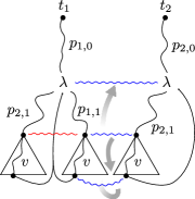
Figure 7. Schematic picture of the proof of Theorem A.1. Blue connections denote bisimilarity, red a single fork.

The sections that follow will further flesh out the details of these high-level descriptions.

A.1. Bisimilarity implies Fork Equivalence

We start with some preliminary observations and lemmas about the sets $\mathbb{P}\!\left(\cdot\right)$, $\mathbb{V}\!\left(\cdot\right)$ and $\mathbb{F}\!\left(\cdot\right)$ and how they relate to term indexing.

Observation A.4.

Various subsets of term paths can be derived from the paths of its subterms:

$$\mathbb{P}\!\left(\lambda\ t\right) =\{\downarrow p\mid p\in\mathbb{P}\!\left(t\right)\}\cup\{\varepsilon\} \mathbb{P}\!\left(t\ u\right) =\{\swarrow p\mid p\in\mathbb{P}\!\left(t\right)\} \cup\{\searrow p\mid p\in\mathbb{P}\!\left(u\right)\}\cup\{\varepsilon\}$$

$$\mathbb{V}\!\left(\lambda\ t\right) =\{\downarrow p\mid p\in\mathbb{V}\!\left(t\right)\} \mathbb{V}\!\left(t\ u\right) =\{\swarrow p\mid p\in\mathbb{V}\!\left(t\right)\} \cup\{\searrow p\mid p\in\mathbb{V}\!\left(u\right)\}$$

$$\mathbb{F}\!\left(\lambda\ t\right) =\{\downarrow p\mid p\in\mathbb{F}\!\left(t\right)\wedge t[p]\neq\underline{\left|p\right|_{\lambda}}\}\quad \mathbb{F}\!\left(t\ u\right) =\{\swarrow p\mid p\in\mathbb{F}\!\left(t\right)\} \cup\{\searrow p\mid p\in\mathbb{F}\!\left(u\right)\}$$

Lemma A.5.

If $p\in\mathbb{P}\!\left(t\right)$ then $\mathbb{P}\!\left(t\right)=\mathbb{P}\!\left(t[p]\right)$ implies $p=\varepsilon$.

Proof.

By induction on $p$, using Observation A.4. ∎

The next three preliminary lemmas state that if two term nodes are bisimilar, then the position sets $\mathbb{P}\!\left(\cdot\right)$, $\mathbb{V}\!\left(\cdot\right)$, $\mathbb{F}\!\left(\cdot\right)$ and $\mathbb{B}\!\left(\cdot\right)$ of their subjects must be equal. These lemmas are important, because they show that bisimilar nodes have largely the same structure. One can see the set $\mathbb{P}\!\left(t\right)$ as the “skeleton” of $t$, where the contents of leafs (variables) are ignored. If subjects do not have the same skeleton, there is no hope of forming a bisimulation between them.

Lemma A.6.

If $t_{1}\llbracket p_{1}\rrbracket\sim_{\text{b}}t_{2}\llbracket p_{2}\rrbracket$ then $\mathbb{P}\!\left(t_{1}[p_{1}]\right)=\mathbb{P}\!\left(t_{2}[p_{2}]\right)$.

Proof.

We have a bisimulation $R$ with $(t_{1}\llbracket p_{1}\rrbracket,t_{2}\llbracket p_{2}\rrbracket)\in R$. Proceed by induction on $t_{1}[p_{1}]$.

Case $t_{1}[p_{1}]=\underline{i}$::

Relation $R$ mandates that there exists $j$ such that $t_{2}[p_{2}]=\underline{j}$. The conclusion is then trivially true.

Case $t_{1}[p_{1}]=\lambda\ u$::

We have $t_{1}\llbracket p_{1}\rrbracket\overset{\downarrow}{\longrightarrow}t_{1}\llbracket p_{1}\downarrow\rrbracket$. Furthermore, from $R$, we have that $t_{2}\llbracket p_{2}\rrbracket\overset{\downarrow}{\longrightarrow}t_{2}\llbracket p_{2}\downarrow\rrbracket$. The induction hypothesis then gives us $\mathbb{P}\!\left(t[p_{1}\downarrow]\right)=\mathbb{P}\!\left(t[p_{2}\downarrow]\right)$. Finally, we conclude $\mathbb{P}\!\left(t[p_{1}]\right)=\mathbb{P}\!\left(t[p_{2}]\right)$ with the help of Observation A.4.

Case $t_{1}[p_{1}]=u\ v$::

Analogous to the previous case.∎

Whereas the previous lemma shows that bisimilar subjects must have equal skeletons, the next lemma shows that their variables must also be related. In the introduction, we showed that the de Bruijn indices of bisimilar subjects are not always equal. Nevertheless, positions that represent free variables in one subject must also be free positions in the other subject. (The same fact holds for bound variables because $\mathbb{B}\!\left(\cdot\right)$ is the complement of $\mathbb{F}\!\left(\cdot\right)$.)

Lemma A.7.

If $t_{1}\llbracket p_{1}\rrbracket\sim_{\text{b}}t_{2}\llbracket p_{2}\rrbracket$ then $\mathbb{F}\!\left(t_{1}[p_{1}]\right)=\mathbb{F}\!\left(t_{2}[p_{2}]\right)$.

Proof.

We have a bisimulation $R$ with $(t_{1}\llbracket p_{1}\rrbracket,t_{2}\llbracket p_{2}\rrbracket)\in R$. Proceed by induction on $t_{1}[p_{1}]$. Cases for variables and application proceed straightforward. The interesting case occurs when $t_{1}[p_{1}]=\lambda\ u$. From $R$ and the induction hypothesis, we obtain $\mathbb{F}\!\left(t_{1}[p_{1}\downarrow]\right)=\mathbb{F}\!\left(t_{2}[p_{2}\downarrow]\right)$. Observation A.4 shows that it now suffices to prove

$$\{q\mid q\in\mathbb{F}\!\left(t_{1}[p_{1}\downarrow]\right)\wedge t_{1}[p_{1}\downarrow q]\neq\underline{\left|q\right|_{\lambda}}\}=\{q\mid q\in\mathbb{F}\!\left(t_{2}[p_{2}\downarrow]\right)\wedge t_{2}[p_{2}\downarrow q]\neq\underline{\left|q\right|_{\lambda}\}}.$$

In other words, it suffices to prove that if $q\in\mathbb{F}\!\left(t_{1}[p_{1}\downarrow]\right)$ and $t_{1}[p_{1}\downarrow q]=\underline{\left|q\right|_{\lambda}}$, then $t_{2}[p_{2}\downarrow q]=\underline{\left|q\right|_{\lambda}}$. Without loss of generality, we assume $t_{2}[p_{2}\downarrow q]<\underline{\left|q\right|_{\lambda}}$ to obtain a contradiction. We can then make a split $q=q_{0}\downarrow q_{1}$ such that

$$t_{2}\llbracket p_{2}\rrbracket\sim_{\text{b}}t_{1}\llbracket p_{1}\rrbracket\sim_{\text{b}}t_{2}\llbracket p_{2}\downarrow q_{0}\downarrow\rrbracket.$$

Then, from Lemma A.6 we have $\mathbb{P}\!\left(t_{2}[p_{2}]\right)=\mathbb{P}\!\left(t_{2}[p_{2}\downarrow q_{0}\downarrow]\right)$. Finally, Lemma A.5 gives a contradiction. ∎

Next is a lemma that shows that if two subjects are bisimilar, their sub-structures must also be bisimilar. This is the analogous lemma to Observation 2.5 for fork equivalence.

Lemma A.8.

If $q\in\mathbb{P}\!\left(t_{1}[p_{1}]\right)$ and $t_{1}\llbracket p_{1}\rrbracket\sim_{\text{b}}t_{2}\llbracket p_{2}\rrbracket$ then $t_{1}\llbracket p_{1}q\rrbracket\sim_{\text{b}}t_{2}\llbracket p_{2}q\rrbracket$.

Proof.

Straightforward by induction on $q$. ∎

As a final preliminary lemma, we note that if the subject of a term node is closed, then its context is irrelevant. This is shown by establishing a bisimulation relation between the node, and a modification such that the context is thrown away.

Lemma A.9.

If $t$ and $t[p]$ are closed, then $t\llbracket p\rrbracket\sim_{\text{b}}t[p]\llbracket\varepsilon\rrbracket$.

Proof.

Construct the relation

$$R=\{(t\llbracket pq\rrbracket,t[p]\llbracket q\rrbracket)\mid q\in\mathbb{P}\!\left(t[p]\right)\}.$$

Verifying that $R$ is a bisimulation relation is straightforward. The only case of note is when $t[pq]$ is a variable. We know that the binder corresponding to the variable is a subterm of $t[p]$, because that term is closed. Hence, we can verify that this binder is bisimilar to itself under $R$. ∎

We are now ready to prove the main technical “workhorse” lemma for this section. The following lemma extracts the required information for a bisimulation relation in order to establish a single fork. The conclusion of this lemma corresponds closely to the required conditions in Definition 2.4 to build a single fork. Note that the addition of the index into position $r$ is a technical requirement to make the induction hypothesis sufficiently strong. When the lemma is used, we always set $r=\varepsilon$.

Lemma A.10.

If $t\llbracket pq_{1}\rrbracket\sim_{\text{b}}t\llbracket pq_{2}\rrbracket$ and $q_{1}$ is locally closed in $t[p]$, then $t[p]\langle q_{1}\rangle[r]=t[p]\langle q_{2}\rangle[r]$.

Proof.

Note that from Lemma A.8 we have

(0.6) $$t\llbracket pq_{1}r\rrbracket\sim_{\text{b}}t\llbracket pq_{2}r\rrbracket.$$

Proceed by induction on $t[pq_{1}r]$. In case $t[pq_{1}r]$ is a variable, we perform additional case analysis on wether $r$ is bound or free.

Case $t[pq_{1}r]=\underline{i}$ such that $r\in\mathbb{F}\!\left(t[pq_{1}]\right)$::

Because $r$ is free, and $q_{1}$ is locally closed in $t[p]$, we know that $q_{1}r\in\mathbb{F}\!\left(t[p]\right)$. Therefore, there exists a split $p=p_{1}\downarrow p_{2}$ such that

$$t\llbracket p_{1}\downarrow p_{2}q_{1}r\rrbracket\overset{\uparrow}{\longrightarrow}t\llbracket p_{1}\rrbracket.$$

The bisimulation relation from Equation 0.6 additionally mandates that $t[pq_{2}r]=\underline{j}$ for some $j$. Without loss of generality, assume $i\leq j$. We then know that there exists $s$ such that t⟦pq_2r⟧ ↑⟶t⟦p_1s⟧ t⟦p_1⟧ ∼_bt⟦p_1s⟧. From Lemma A.6 and Lemma A.5 we then have $s=\varepsilon$, and as such t[pq_1r] = —p_2q_1r—_λ t[pq_2r] = —p_2q_2r—_λ. We then conclude that

$$t[p]\langle q_{1}\rangle[r]=\underline{\left|p_{2}q_{1}r\right|_{\lambda}-\left|q_{1}\right|_{\lambda}}=\underline{\left|p_{2}q_{2}r\right|_{\lambda}-\left|q_{2}\right|_{\lambda}}=t[p]\langle q_{2}\rangle[r].$$

Case $t[pq_{1}r]=\underline{i}$ such that $r\in\mathbb{B}\!\left(t[pq_{1}]\right)$::

From the main bisimulation hypothesis and Lemma A.7 we have $\mathbb{F}\!\left(t[pq_{1}]\right)=\mathbb{F}\!\left(t[pq_{2}]\right)$. Since $\mathbb{B}\!\left(\cdot\right)$ is the complement of $\mathbb{F}\!\left(\cdot\right)$, we know that $r\in\mathbb{B}\!\left(t[pq_{2}]\right)$. The bisimulation relation from Equation 0.6 then mandates that there exist two splits $r=r_{1A}\downarrow r_{1B}=r_{2A}\downarrow r_{2B}$ such that t[pq_1r] = —r_1B—_λ t[pq_2r] = —r_2B—_λ t⟦pq_1r_1A⟧ ∼_bt⟦pq_2r_2A⟧. Moreover, from Lemma A.6 we have $\mathbb{P}\!\left(t[pq_{1}r_{1A}]\right)=\mathbb{P}\!\left(t[pq_{2}r_{2A}]\right)$. Now, without loss of generality, assume $|r_{1A}|\geq|r_{2A}|$. We can then make an additional split $r_{1A}=r_{2A}s$, giving us P​(t[pq_1r_2A s]