Analytical solution of the Poiseuille flow of a De Kee viscoplastic fluid
Abstract
We provide an explicit analytical solution of the planar Poiseuille flow of a viscoplastic fluid governed by the constitutive equation proposed by De Kee and Turcotte (Chem. Eng. Commun. 6 (1980) 273--282). Formulae for the velocity and the flow rate are derived, making use of the Lambert W function. It is shown that a solution does not always exist because the flow curve is bounded from above and hence the rheological model can accommodate stresses only up to a certain limit. In fact, the flow curve reaches a peak at a critical shear rate, beyond which it exhibits a negative slope, giving rise to unstable solutions.
1 Introduction
Viscoplastic fluids are characterised by the property of behaving in a solid-like manner when the applied stress is below a limit value called the yield stress [1, 2]. Examples of such fluids include toothpaste, hair gel, mayonnaise, shaving foam, mud, mucus, clay, fresh concrete, crude oil, and many others. This class of fluids includes a variety of materials such as foams, emulsions, colloids, and physical gels, with the emergence of yield stress as a macroscopic property being attributable to a variety of microscopic mechanisms, possibly different for each material type [3].
Mathematical modelling of the rheological behaviour of viscoplastic fluids is a field that has been developing during the last century or so. Classic viscoplastic models originate in the work of Eugene Bingham who proposed the famous constitutive model that carries his name [4]. These models, commonly called simple yield stress fluids, assume the material to have a solid state that is completely rigid, and a fluid state which is that of a generalised Newtonian fluid. The most popular such model, which incorporates both a yield stress and shear thinning or thickening, is the Herschel-Bulkley (HB) model [5]:
| (1) |
where is the rate-of-strain tensor and is its magnitude, is the deviatoric stress tensor and is its magnitude, is the yield stress, is the consistency index, and the exponent determines if the fluid is shear-thinning () or shear-thickening (). For the Herschel-Bulkley model reduces to the Bingham model. Another popular model of this class is the Casson model [6].
Real viscoplastic fluids exhibit additional rheological properties such as elasticity and thixotropy [7, 8], a fact that has given rise to recent efforts for the development of more complicated rheological models with expanded physics [9, 10, 11]. Nevertheless, simple yield stress fluids continue to be used at present and will most likely persist in the future, having the advantages of simplicity and focus on plasticity and shear-thinning, which are the defining aspects of many flows of interest. A recent defence of this class of rheological models is provided in [12].
Simple yield stress fluids are challenging from mathematical and computational perspectives. The stress tensor is indeterminate in the unyielded (solid-state) regions, while the evolution of the yield surfaces (the boundaries between the yielded and unyielded material) is not described explicitly by some equation. Several numerical methods have been developed for solving the flows of simple yield stress fluids [13, 14, 15], some of which solve the original models directly while others first regularise them, effectively converting the unyielded material into a very viscous fluid (something that may also have some physical justification, at least for some materials). The most popular regularisation method is that of Papanastasiou [16].
A less popular simple yield stress fluid model was proposed by De Kee and Turcotte [17]:
| (2) |
Compared to the Herschel-Bulkley model (1), instead of the consistency and the power-law exponent , the De Kee model employs constants and which have units of viscosity and time, respectively. For our analysis, it is convenient to define also the reciprocal of the time constant as , which has dimensions of strain rate, because, as will be shown, this is a critical value of strain-rate that delimits distinct regions where the properties of the model differ drastically. Like the Herschel-Bulkley model, the De Kee model can predict both plasticity and shear-thinning.
In a later work [18], De Kee and co-workers presented a Papanastasiou-type regularised version of the model in order to bound the viscosity at vanishing shear rate. Since the viscous component is already bounded -- which is an advantage of the De Kee model over the HB model -- the regularisation needs to be applied only to the plastic component (nevertheless, it should be pointed out that the HB viscosity is easily bounded by applying the regularisation also to the viscous component [19, 20]). Another advantage of the De Kee model is that the dimensions of its constants, and , are fixed, and they have a clear physical significance, in contrast to the HB parameters where the dimensions of the consistency depend on .
The De Kee -- Turcotte model has been used in various experimental and numerical studies. Kaczmarczyk et al. [21] fitted the model (2), incorporating additional viscous terms and , to rheological measurements for Plantago ovata water extract solutions. They examined both dilute (zero yield stress) and semi-dilute (non-zero yield stress) solutions. Yahia and Khayat [22] made rheological measurements on cement grout and found that the De Kee model is suitable for mixtures made of 100% cement and rheology-modifying admixtures. Seo et al. [23] proposed a generalised model for electrorheological fluids which reduces to the De Kee -- Turcotte model for particular choices of parameters. The regularized version of the model [18] was used by Zare et al. [24] to model polymer blends and nanocomposites containing poly (lactic acid), poly (ethylene oxide) and carbon nanotubes. In numerical studies, the model was used for the numerical simulation of the cessation of viscoplastic Couette flow [25] and the numerical simulation of the flow in a rheometer with concentric cylinder geometry [26].
The present work exposes an inherent limitation of the model: it only yields solutions within limited parameter ranges. This limitation is due to its excessive shear thinning. As an application, we will solve analytically the planar Poiseuille flow and determine the range of parameters for which a solution exists. The solution is obtained with the use of the Lambert W function [27], which has proved quite useful in non-Newtonian fluid mechanics. This function is briefly presented in Section 2. The aforementioned limitation of the model is exposed in Section 3, and the analytical solutions, both stable and unstable, of planar Poiseuille flow are presented in Section 4.
2 The Lambert W function
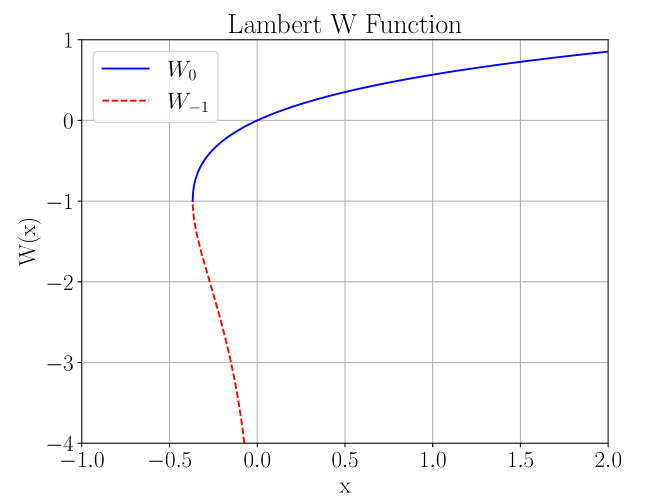
Our analytical solution makes use of the Lambert W function, which returns the solution of the equation :
| (3) |
The function is plotted in Fig. 1. It is multivalued in the interval , and therefore consists of two branches: the principle branch, denoted by , for , and the secondary branch, denoted as , for . These branches are illustrated in Fig. 1; the principal branch is strictly increasing from to infinity, while the secondary branch is strictly decreasing from to minus infinity. It is important to note that the equation (3) does not have a solution for . Hence, is not defined for .
An overview of the Lambert W function and its applications can be found in [27]. The function is useful in Newtonian fluid mechanics [28], and more so in non-Newtonian fluid mechanics where it has many applications [29, 30].
Some integrals involving the Lambert function that are useful for the present application are:
| (4) |
| (5) |
| (6) |
where is an arbitrary constant of integration. All of these expressions can be obtained by making the substitution , and then repeatedly performing integration by parts.
3 Flow curve
Figures 2 and 3 illustrate the variation of stress and viscosity, respectively, with shear rate, for the De Kee -- Turcotte model. Plot 2 is obtained by taking the norm of Eq. (2). In plot 3 only the ‘‘viscous’’ part, , of the viscosity is considered -- the ‘‘plastic’’ part, , is omitted.
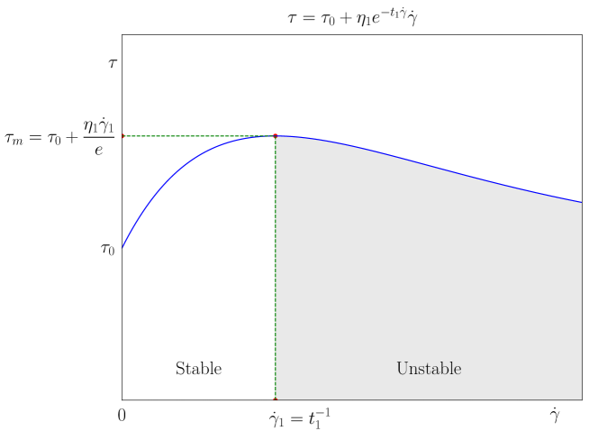
What is immediately striking in Fig. 2 is that is not a strictly increasing function, but has a maximum of at . This is due to the excessive shear-thinning for , which causes not only the viscosity, but even the stress itself, to fall. This has the following repercussions.
Firstly, the stress cannot increase beyond the value . This means that there are many cases for which steady-state solutions do not exist because the momentum balance would require higher stress values than the model can provide. One example is Poiseuille flows whose pressure gradient exceeds a certain threshold, a case that will be examined shortly.
Secondly, for those cases that a solution exists, we can see that the same stress state can be achieved with two different values of the shear rate -- that is, for each value of the corresponding horizontal line in Fig. 2 intersects the curve at two points, say and . Hence, we expect multiple solutions, when they exist. Of these solutions, those with shear rates will be unstable [31] because any perturbation in will cause the stress to change in such a direction that will amplify further the change in the shear rate, starting a vicious circle. If is increased, falls and the reduced viscous resistance in the fluid will cause a further increase in and so on. The opposite will happen if is perturbed in the negative direction: this will cause to increase, strengthening the viscous resistance to the flow and causing further decrease to etc. These features of the model will be demonstrated in the case of planar Poiseuille flow in the next section.
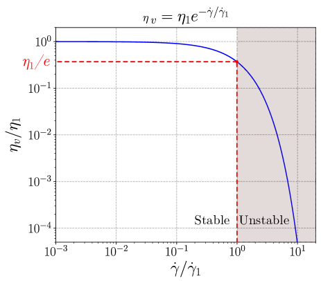
Concerning the viscosity, Fig. 3 seems like a typical shear-thinning viscosity curve. At low shear rates, , the ‘‘viscous’’ contribution to the viscosity, , is approximately constant and equal to , with the model exhibiting an almost Newtonian behaviour, in contrast to the component of the HB viscosity which becomes infinite at vanishing shear rate. At this viscosity component has decreased to . Beyond the shear thinning intensifies dramatically. However, it should be noted that lies in the unstable regime and therefore the lowest practically achievable viscosity is with viscosities lower than that being practically impossible to achieve. In other words, practically .
4 Planar Poiseuille flow
With these considerations, let us proceed to the analytical solution of planar Poiseuille flow.
4.1 Preliminary considerations
For simple shear flow, the De Kee model (2) reduces to the following form:
| (7) |
where is the flow direction and is the velocity in that direction, is the perpendicular direction across which varies, and is the shear stress.
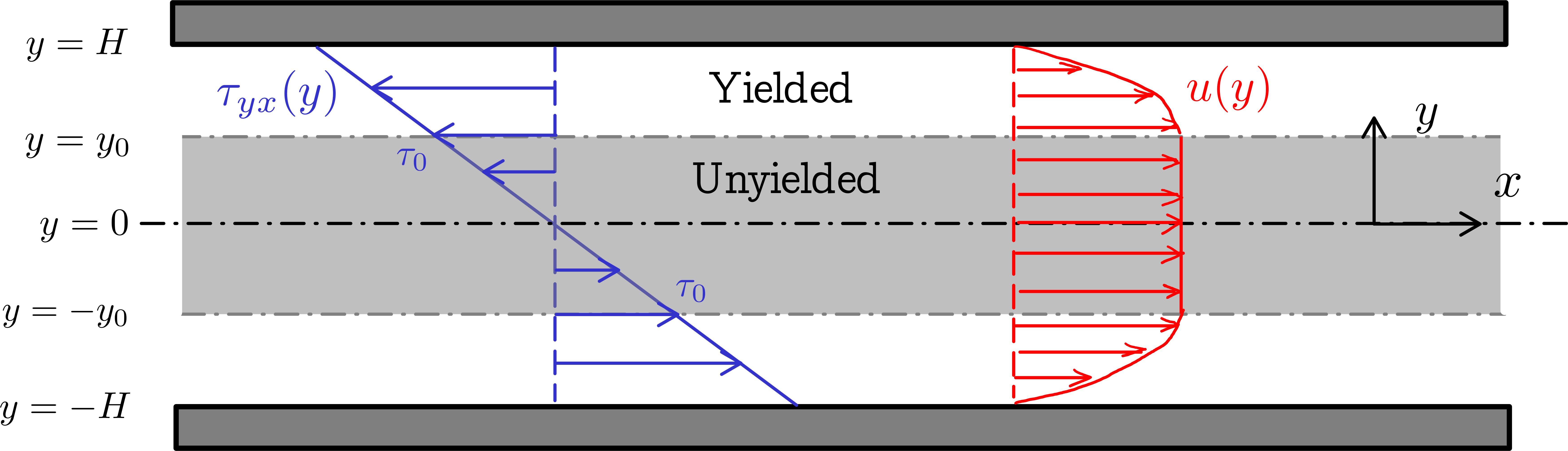
One such flow is planar Poiseuille flow, a steady flow where fluid is pushed along a channel formed by two infinite horizontal parallel plates, located at a distance apart, by an imposed pressure gradient, (Fig. 4). For this flow, the momentum balance (Cauchy equation) reduces to:
| (8) |
where is set midway between the plates (Fig. 4). The stress grows linearly with distance from the midplane, ranging from zero at the midplane to a maximum magnitude of at the plates. Therefore, as long as , an unyielded core will form in the middle of the domain, up to a distance of
| (9) |
from the midplane (from Eq. (8)). If then obviously no flow will occur and the whole material will be unyielded, provided that no-slip conditions apply at the plates, which is an assumption that will be made in the present paper. Otherwise, if , then there will be a yielded zone in and flow will occur. We can therefore focus on the partially yielded case and first consider the yielded zone, where we can substitute Eq. (7) in Eq. (8); in the upper half () of the domain, where , this substitution gives
| (10) |
This can be easily manipulated into the form
| (11) |
Applying the Lambert function to both sides and rearranging we get
| (12) |
The left-hand side, , is negative, and hence the output of the Lambert function on the right-hand side must also be negative, which requires that its argument is negative (Fig. 1). This is indeed the case, as the occurrence of flow means that (Eq. (8)). But this means that we are in the region where has two branches, and hence there are two solutions to Eq. (12), one employing and one employing . We will examine this issue later, but for now let us proceed without particularising the branch that is selected.
According to what was said in Sec. 2, in order for Eq. (12) to have a solution, the argument of the Lambert function must be greater than or equal to . This argument is negative, and its magnitude is maximised at . Therefore, the existence of a solution requires that
| (13) |
Now, from Eq. (8), is the maximum stress value, required at the plates so that the pressure gradient is counterbalanced and the flow is steady. Therefore, Eq. (13) is equivalent to the condition
| (14) |
which simply says that the stress should be everywhere smaller than the maximum value producible by the De Kee -- Turcotte model, as shown in Sec. 3. If the pressure gradient is too large for to counteract it (i.e. condition (13) is not satisfied), then steady-state flow is not possible.
4.2 Velocity profile
Assuming that the pressure gradient is sufficiently small to satisfy condition (13), we will proceed with the integration of Eq. (12). For convenience, it will be brought to non-dimensional form by employing the following non-dimensionalisation:
| (15) |
We will also substitute (Eq. (9)). The non-dimensional form of (12) is then:
| (16) |
This can be integrated using Eq. (4), while the constant of integration can be determined by the boundary condition , to arrive at the following velocity profile for the yielded region:
| (17) | ||||
In the unyielded region the velocity is uniform and equal to that of the yielded region at :
| (18) |
At this point, it is pertinent to consider the issue of the branches of . Returning to Eq. (12), we note the following.
Principal branch
With increasing , i.e. closer to the wall, the argument of in Eq. (12) becomes more negative, and hence increases (Fig. 1), implying that also increases (Eq. (12)). This is normal behaviour: higher velocity gradients develop near the walls; it is because higher stresses require higher velocity gradients in the stable region.
On the other hand, considering what happens when , due to Eq. (9) the argument of in Eq. (12) tends to zero, and so does itself, so that the velocity gradient is zero at the yield surface -- again, normal behaviour exhibited by other viscoplastic models as well. Stress continuity at the yield surface requires that the viscous part of the stress reduces towards zero, leaving only the plastic part, as we approach the yield surface from the yielded side.
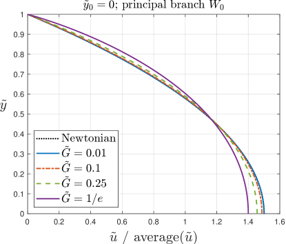
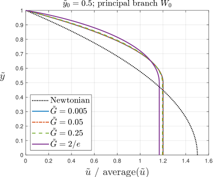
Velocity profiles for cases without yield stress () and with yield stress () are shown in Figs. 5(a) and 6(a), respectively, for various values of dimensionless pressure gradient , up to the maximum allowable for steady-state attainment ( for and for ). The maximum allowable dimensionless pressure gradient is obtained by substituting in the condition (13) and non-dimensionalising it to get:
| (19) |
Secondary branch
With increasing , i.e. closer to the wall, the argument of in Eq. (12) becomes more negative, and hence decreases (Fig. 1), implying that decreases as well (Eq. (12)). This is the opposite of what is normally expected, but due to being a decreasing function in the unstable region (Fig. 2), in order to get the needed higher stresses near the wall the shear rate has to decrease there.
Again counterintuitively, when , due to Eq. (9) the argument of in Eq. (12) tends to zero, and tends to , so that the velocity gradient becomes infinite at the yield surface.
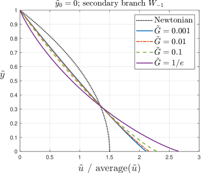
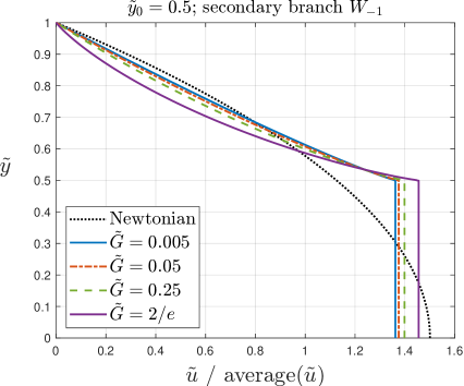
Velocity profiles for cases without yield stress () and with yield stress () are shown in Figs. 5(b) and 6(b), respectively, for various values of dimensionless pressure gradient , up to the maximum allowable for steady-state attainment. Of course, these solutions are unstable. The plots seem to show finite values of the velocity gradient (16) at instead of the theoretical infinite one, but this is due to the slowness of the decrease of towards as . For example, for , which is a typical -value resolution for drawing the plots, Eq. (16) gives a dimensionless velocity gradient of for and for (note also that the slopes in Figs. 5(b) and 6(b) are not to scale, because the velocities have been normalized by their average values).
4.3 Flow rate
When a solution exists, the flow rate, per unit width, can be calculated by integrating the velocity across the height of the channel:
| (20) |
where the symmetry about the plane has been exploited. Also, it will be convenient to non-dimensionalise the flow rate:
| (21) |
where, for convenience, the steady velocity (18) of the unyielded plug is denoted as . With this notation, the velocity in the yielded region can be written as
| (22) |
and the above integral becomes
| (23) | ||||
This can be evaluated with the help of Eqs. (5) and (6), to obtain
| (24) | ||||
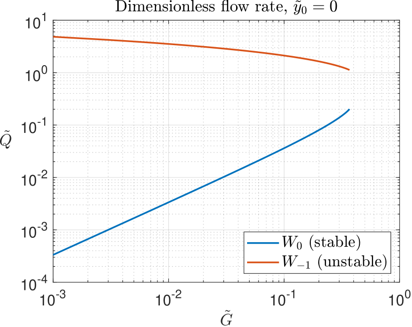
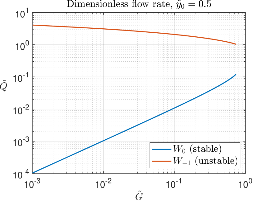
where . Because and , the term equals for the stable branch and for the unstable one. Figure 7 shows plots of the dimensionless flow rate as a function of the dimensionless pressure gradient for (no yield stress) and . Note that in the latter case, since is held constant in Fig. 7(b) irrespective of , the curve should not be construed as varying the pressure gradient in a fixed channel with a fixed fluid, but in order for to remain constant as the pressure gradient varies the yield stress of the fluid must vary simultaneously with (from Eq. (9) we get where ).
5 Conclusions
The De Kee -- Turcotte model has the advantages of the physical significance of its parameters and its viscous plateau at low shear rates. On the other hand, its exponential shear-thinning limits its range of applicability: it bounds the magnitude of the stress that it can produce, making it unusable in high-stress flows. Furthermore, its flow curve exhibits a maximum which splits it into a stable (stress-increasing) part and an unstable (stress-decreasing) part. The behaviour of the model in the stable region is akin to the other simple viscoplastic models, such as the Herschel-Bulkley. An analytical solution was given for planar Poiseuille flow in terms of the Lambert W function.
Ironically, the model’s exponential shear-thinning behaviour with the resulting limitation that it imposes on the model allows solutions only in cases with mild shear-thinning. Hence, the velocity profiles in Figs. 5(a) and 6(a) are reminiscent of mildly shear-thinning power-law and Herschel-Bulkley profiles. However, power-law and Herschel-Bulkley fluids can undergo much more shear-thinning than a De Kee fluid. In any case the viscosity cannot drop below of its zero-shear-rate value if we are to remain in the stable region (Fig. 3).
One can try to increase the range of applicability by decreasing the time constant (increasing the critical rate of strain ), but this will expand the Newtonian plateau (Fig. 3) making the fluid more Newtonian (or more Bingham-like in the viscoplastic case). On the other hand, another possibility for extending the model’s range of applicability would be to incorporate multiple viscous components [17, 21]. Also, we did not discuss the shear-thickening case, which is achieved by using negative time constants (critical rates-of-strain ). In this case the stress can grow without bound and the limitation vanishes. For the Poiseuille flow, this has the implication that in Eq. (12) the argument of the function is now positive and therefore there are no limitations concerning its magnitude (Fig. 1).
The non-monotonicity of the De Kee flow curve establishes the existence of unstable solutions alongside the stable ones, whenever there are solutions at all. The unstable velocity profiles in planar Poiseuille flow were seen to exhibit inverted and unrealistic features compared to the stable ones.
References
- [1] P. Coussot, ‘‘Bingham’s heritage,’’ Rheologica Acta, vol. 56, pp. 163--176, 2017.
- [2] N. J. Balmforth, I. A. Frigaard, and G. Ovarlez, ‘‘Yielding to stress: Recent developments in viscoplastic fluid mechanics,’’ Annual Review of Fluid Mechanics, vol. 46, pp. 121--146, 2014.
- [3] D. Bonn, M. M. Denn, L. Berthier, T. Divoux, and S. Manneville, ‘‘Yield stress materials in soft condensed matter,’’ Reviews of Modern Physics, vol. 89, 2017.
- [4] E. C. Bingham, Fluidity and Plasticity. McGraw-Hill, 1922.
- [5] W. H. Herschel and R. Bulkley, ‘‘Konsistenzmessungen von gummi-benzollösungen,’’ Kolloid-Zeitschrift, vol. 39, pp. 291--300, 1926.
- [6] N. Casson, ‘‘Flow equation for pigment-oil suspensions of the printing ink-type,’’ Rheology of disperse systems, pp. 84--104, 1959.
- [7] M. Dinkgreve, M. M. Denn, and D. Bonn, ‘‘“Everything flows?”: elastic effects on startup flows of yield-stress fluids,’’ Rheologica Acta, vol. 56, no. 3, pp. 189--194, 2017.
- [8] R. G. Larson and Y. Wei, ‘‘A review of thixotropy and its rheological modeling,’’ Journal of Rheology, vol. 63, no. 3, pp. 477--501, 2019.
- [9] P. Saramito, ‘‘A new elastoviscoplastic model based on the herschel–bulkley viscoplastic model,’’ Journal of Non-Newtonian Fluid Mechanics, vol. 158, no. 1–3, pp. 154--161, 2009.
- [10] C. J. Dimitriou and G. H. McKinley, ‘‘A canonical framework for modeling elasto-viscoplasticity in complex fluids,’’ Journal of Non-Newtonian Fluid Mechanics, vol. 265, pp. 116--132, 2019.
- [11] S. Varchanis, G. Makrigiorgos, P. Moschopoulos, Y. Dimakopoulos, and J. Tsamopoulos, ‘‘Modeling the rheology of thixotropic elasto-visco-plastic materials,’’ Journal of Rheology, vol. 63, no. 4, pp. 609--639, 2019.
- [12] I. Frigaard, ‘‘Simple yield stress fluids,’’ Current Opinion in Colloid & Interface Science, vol. 43, pp. 80--93, 2019.
- [13] E. Mitsoulis and J. Tsamopoulos, ‘‘Numerical simulations of complex yield-stress fluid flows,’’ Rheologica Acta, vol. 56, no. 3, pp. 231--258, 2017.
- [14] P. Saramito and A. Wachs, ‘‘Progress in numerical simulation of yield stress fluid flows,’’ Rheologica Acta, vol. 56, no. 3, pp. 211--230, 2017.
- [15] P. Moschopoulos, S. Varchanis, A. Syrakos, Y. Dimakopoulos, and J. Tsamopoulos, ‘‘S-pal: A stabilized finite element formulation for computing viscoplastic flows,’’ Journal of Non-Newtonian Fluid Mechanics, vol. 309, p. 104883, Nov. 2022.
- [16] T. C. Papanastasiou, ‘‘Flows of materials with yield,’’ Journal of Rheology, vol. 31, no. 5, pp. 385--404, 1987.
- [17] D. De Kee and G. Turcotte, ‘‘Viscosity of biomaterials,’’ Chemical Engineering Communications, vol. 6, no. 4–5, pp. 273--282, 1980.
- [18] H. Zhu, Y. Kim, and D. De Kee, ‘‘Non-Newtonian fluids with a yield stress,’’ Journal of Non-Newtonian Fluid Mechanics, vol. 129, no. 3, pp. 177--181, 2005.
- [19] K. Sverdrup, N. Nikiforakis, and A. Almgren, ‘‘Highly parallelisable simulations of time-dependent viscoplastic fluid flow with structured adaptive mesh refinement,’’ Physics of Fluids, vol. 30, no. 9, 2018.
- [20] A. Syrakos, Y. Dimakopoulos, and J. Tsamopoulos, ‘‘A finite volume method for the simulation of elastoviscoplastic flows and its application to the lid-driven cavity case,’’ Journal of Non-Newtonian Fluid Mechanics, vol. 275, p. 104216, 2020.
- [21] K. Kaczmarczyk, J. Kruk, P. Ptaszek, and A. Ptaszek, ‘‘Plantago ovata husk: An investigation of raw aqueous extracts. osmotic, hydrodynamic and complex rheological characterisation,’’ Molecules, vol. 28, no. 4, p. 1660, 2023.
- [22] A. Yahia and K. Khayat, ‘‘Analytical models for estimating yield stress of high-performance pseudoplastic grout,’’ Cement and Concrete Research, vol. 31, no. 5, pp. 731--738, 2001.
- [23] Y. P. Seo, H. J. Choi, and Y. Seo, ‘‘Analysis of the flow behavior of electrorheological fluids with the aligned structure reformation,’’ Polymer, vol. 52, no. 25, pp. 5695--5698, 2011.
- [24] Y. Zare and K. Y. Rhee, ‘‘Modeling of viscosity and complex modulus for poly (lactic acid)/poly (ethylene oxide)/carbon nanotubes nanocomposites assuming yield stress and network breaking time,’’ Composites Part B: Engineering, vol. 156, pp. 100--107, 2019.
- [25] H. Zhu and D. De Kee, ‘‘A numerical study for the cessation of Couette flow of non-Newtonian fluids with a yield stress,’’ Journal of Non-Newtonian Fluid Mechanics, vol. 143, no. 2–3, pp. 64--70, 2007.
- [26] W. Wang, D. De Kee, and D. Khismatullin, ‘‘Numerical simulation of power law and yield stress fluid flows in double concentric cylinder with slotted rotor and vane geometries,’’ Journal of Non-Newtonian Fluid Mechanics, vol. 166, no. 12–13, pp. 734--744, 2011.
- [27] R. M. Corless, G. H. Gonnet, D. E. Hare, D. J. Jeffrey, and D. E. Knuth, ‘‘On the Lambert W function,’’ Advances in Computational mathematics, vol. 5, pp. 329--359, 1996.
- [28] R. Pitsillou, A. Syrakos, and G. C. Georgiou, ‘‘Application of the Lambert W function to steady shearing Newtonian flows with logarithmic wall slip,’’ Physics of Fluids, vol. 32, no. 5, 2020.
- [29] R. Pitsillou, G. C. Georgiou, and R. R. Huilgol, ‘‘On the use of the Lambert function in solving non-Newtonian flow problems,’’ Physics of Fluids, vol. 32, no. 9, 2020.
- [30] R. R. Huilgol and G. C. Georgiou, Fluid Mechanics of Viscoplasticity. Springer International Publishing, 2022.
- [31] J. Yerushalmi, S. Katz, and R. Shinnar, ‘‘The stability of steady shear flows of some viscoelastic fluids,’’ Chemical Engineering Science, vol. 25, no. 12, pp. 1891--1902, 1970.