The Dark Energy Survey: Cosmology Results With $\sim$1500 New High-redshift Type Ia Supernovae Using The Full 5-year Dataset

Abstract

We present cosmological constraints from the sample of Type Ia supernovae (SN Ia) discovered and measured during the full five years of the Dark Energy Survey (DES) Supernova Program. In contrast to most previous cosmological samples, in which supernovae are classified based on their spectra, we classify the DES supernovae using a machine learning algorithm applied to their light curves in four photometric bands. Spectroscopic redshifts are acquired from a dedicated follow-up survey of the host galaxies. After accounting for the likelihood of each supernova being a SN Ia, we find 1635 DES SNe in the redshift-range $0.10<z<1.13$ that pass quality selection criteria and can be used to constrain cosmological parameters. This quintuples the number of high-quality $z>0.5$ SNe compared to the previous leading compilation of Pantheon+, and results in the tightest cosmological constraints achieved by any supernova data set to date. To derive cosmological constraints we combine the DES supernova data with a high-quality external low-redshift sample consisting of 194 SNe Ia spanning $0.025<z<0.10$. Using supernova data alone and including systematic uncertainties we find $\Omega_{\rm M}=0.352\pm 0.017$ in flat-$\Lambda$CDM, and $(\Omega_{\rm M},w)=(0.264^{+0.074}_{-0.096},-0.80^{+0.14}_{-0.16})$ in flat-$w$CDM. For flat-$w_{0}w_{a}$CDM, we find $(\Omega_{\rm M},w_{0},w_{a})=(0.495^{+0.033}_{-0.043},-0.36^{+0.36}_{-0.30},-8.8^{+3.7}_{-4.5})$, consistent with a constant equation of state to within $\sim 2\sigma$. Including Planck CMB data, SDSS BAO data, and DES $3\times 2$-point data gives $(\Omega_{\rm M},w)=(0.321\pm 0.007,-0.941\pm 0.026)$. In all cases dark energy is consistent with a cosmological constant to within $\sim 2\sigma$. In our analysis, systematic errors on cosmological parameters are subdominant compared to statistical errors; these results thus pave the way for future photometrically classified supernova analyses.

DES-2023-805 FERMILAB-PUB-23-0821-PPD

1 Introduction

The standard cosmological model posits that the energy density of the Universe is dominated by dark components that have not been detected in terrestrial experiments and thus do not appear in the standard model of particle physics. Known as cold dark matter and dark energy, their study represents an opportunity to deepen our understanding of fundamental physics.

The Dark Energy Survey (DES) was conceived to characterize the properties of dark matter and dark energy with unprecedented precision and accuracy through four primary observational probes (The Dark Energy Survey Collaboration, 2005; Bernstein et al., 2012; Dark Energy Survey Collaboration, 2016; Lahav et al., 2020). One of these four probes is the Hubble diagram (redshift-distance relation) for Type Ia supernovae (SNe Ia), which act as standardizable candles (Rust, 1974; Pskovskii, 1977; Phillips et al., 1999) to constrain the history of the cosmic expansion rate. To implement this probe, the DES SN survey was designed to provide the largest, most homogeneous sample of high-redshift supernovae ever discovered. The two papers that first presented evidence for the accelerated expansion of the universe (Riess et al., 1998; Perlmutter et al., 1999) used a total of 52 high-redshift supernovae with sparsely sampled light-curve measurements in one or two optical passbands. Building on two decades of subsequent improvements in SN surveys and analysis, we present here the cosmological constraints using the full 5-year DES SN dataset, consisting of well-sampled, precisely calibrated light curves for 1635 new high-redshift supernovae observed in four bands $g,r,i,z$.

For the last decade, SN Ia cosmology constraints have largely come from combining data from many surveys. The recent Pantheon+ analysis (Scolnic et al., 2022; Brout et al., 2022a) combined three separate mid-$z$ samples ($0.1<z<1.0$), 11 different low-$z$ samples ($z<0.1$), and four separate high-$z$ samples ($z>1.0$), each with different photometric systems and selection functions (Gilliland et al., 1999; Hicken et al., 2009; Riess et al., 2001, 2004, 2007; Sullivan et al., 2011; Hicken et al., 2012; Suzuki et al., 2012; Ganeshalingam et al., 2013; Betoule et al., 2014; Krisciunas et al., 2017; Foley et al., 2017; Riess et al., 2018; Sako et al., 2018; Brout et al., 2019b; Smith et al., 2020a). The DES sample, which rivals in number the entirety of Pantheon+, does not have the low-redshift ($z<0.1$) coverage to completely remove the need for external low-$z$ samples, but at higher redshift enables us to replace a heterogeneous mix of samples with a homogeneous sample of high quality, well-calibrated light curves.

A key aim of the DES analysis was to minimize systematic (relative to statistical) errors to enable a robust analysis. Vincenzi et al. (2024) shows that our error budget is dominated by statistical uncertainty, in contrast to most SN cosmology analyses of the last decade, for which the systematic uncertainties equalled or exceeded the statistical uncertainties (Betoule et al., 2014; Scolnic et al., 2018; Dark Energy Survey Collaboration, 2019). We also highlight that the most critical sources of systematics are those related to the lack of a homogeneous and well calibrated low-$z$ sample.

As the DES sample enables a SN Ia measurement of cosmological parameters that is largely independent of previous SN cosmology analyses, we have been careful to “blind” our analysis. The analysis work described in Vincenzi et al. (2024), which stops just short of constraining cosmological parameters, was shared widely with the DES collaboration, evaluated, and approved before unblinding. Unblinding standards included multiple validation checks with simulations and full accounting and explanation of the error budget. No elements of the analysis were changed after unblinding.

In this paper we review the analysis of the complete DES SN dataset (as detailed in many supporting papers; see Fig. 1) and present the cosmological results. An important advance on most previous analyses is that we use a photometrically classified rather than spectroscopically classified sample (Möller & de Boissière, 2020; Qu et al., 2021), and implement advanced techniques to classify SN Ia and incorporate classification probabilities in the cosmological parameter estimation (Kunz et al., 2012; Hlozek et al., 2012). While this advance increases the complexity of the analysis, in this work and previous papers (Vincenzi et al., 2023; Möller et al., 2022) we show that the impact of non-SN Ia contamination due to photometric misclassification is well below the statistical uncertainty on cosmological parameters, and this constitutes one of the key results of our analysis.

Combining our DES data with a low-redshift sample (see Sect. 2), we fit the Hubble diagram to test the standard cosmological model as well as multiple common extensions including spatial curvature, non-vacuum dark energy, and dark energy with an evolving equation of state parameter. In Camilleri et al. (in prep. 2024) we present fits to more exotic models.

The structure of the paper is as follows. We begin in Sec. 2 by describing the dataset, its acquisition, reduction, calibration, and light-curve fitting. We summarize the models we test in Sec. 3 before presenting the results in Sec. 4; our discussion and conclusions follow in Sec. 5 and Sec. 6. The details of our data release, which includes the code needed to reproduce our results, appear in Sánchez (in prep. 2024).

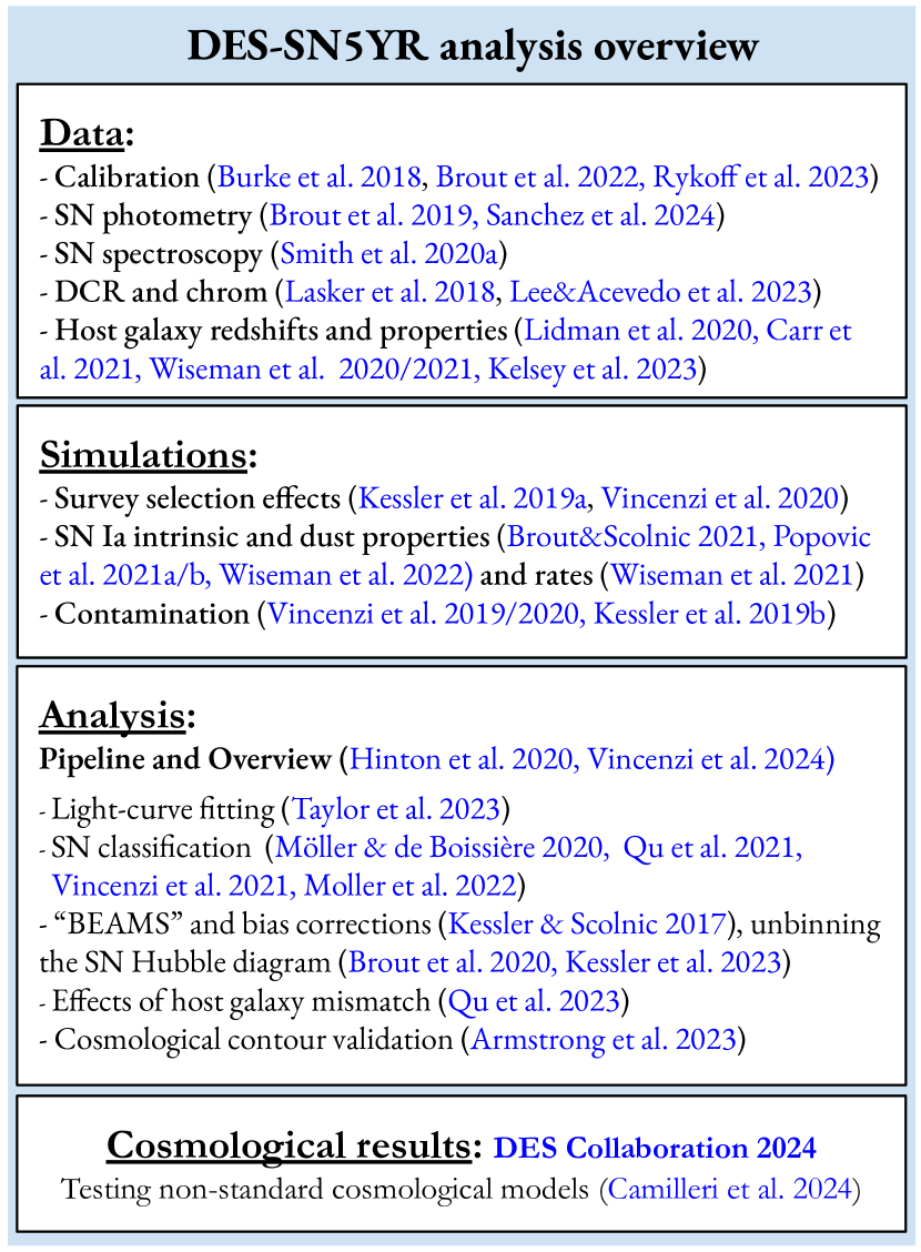
Figure 1: Overview of supporting papers for DES-SN5YR cosmological results.

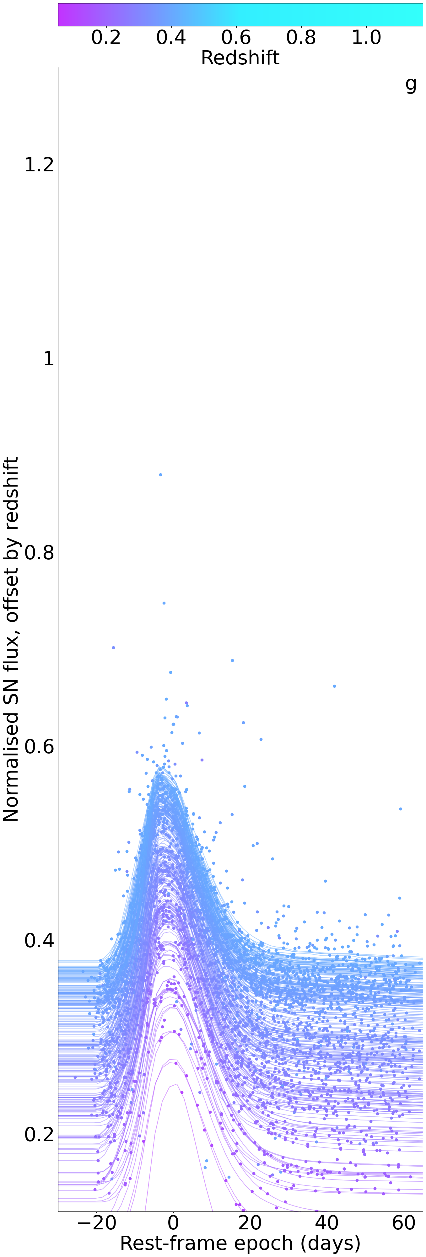
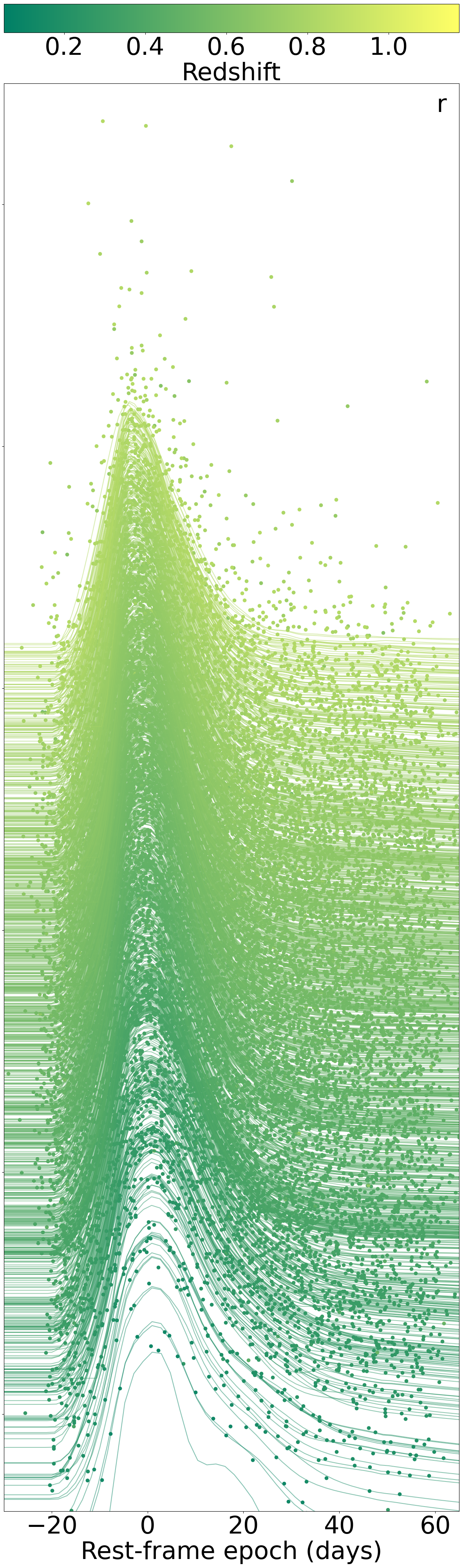
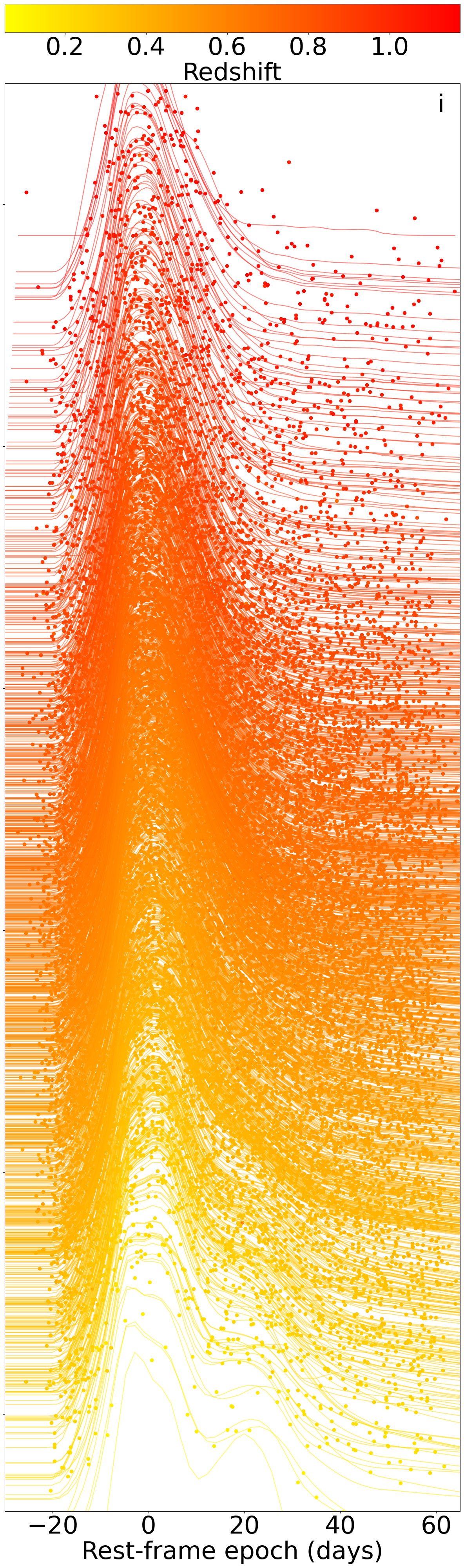
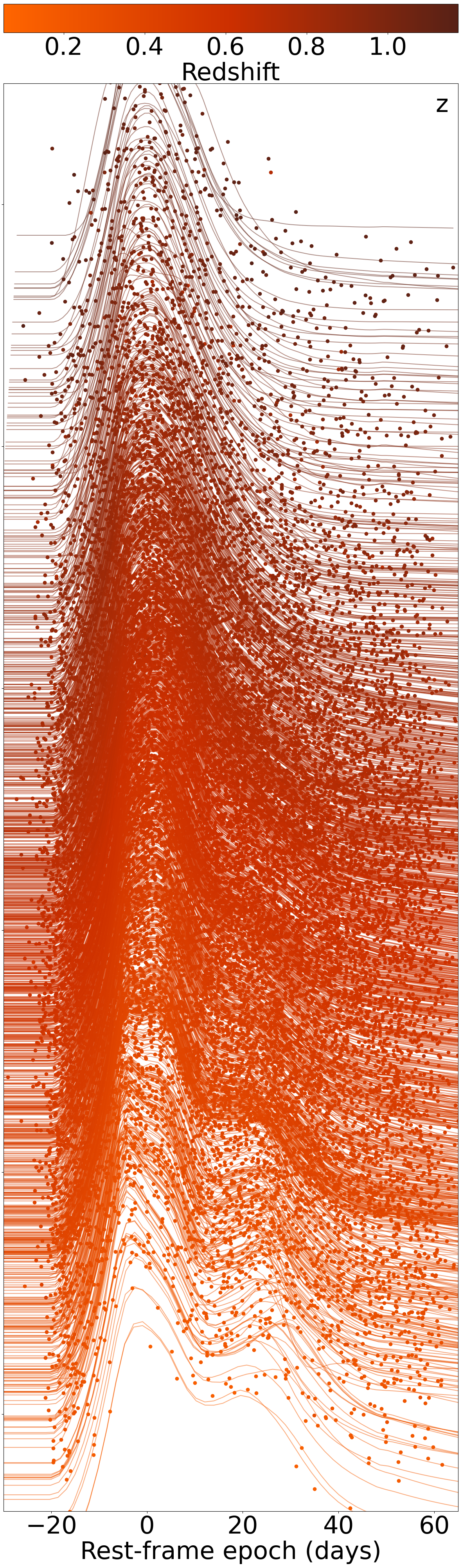
Figure 2: All DES light curves, showing observed magnitudes in $g$, $r$, $i$, and $z$ bands (left to right respectively) normalized by the maximum brightness of each light curve, and with the time-axis de-redshifted to the rest-frame. Each light curve has been arbitrarily offset by their redshift, with higher-redshift objects higher on the plot (as labeled on vertical axis). Lines show best-fit SALT3 light-curve fits. The $g$-band and $r$-band light curves are not used above $z\sim 0.4$ and $z\sim 0.85$ respectively because that corresponds to the redshifts at which the lower-wavelength limit of the SALT3 model ($3500\AA$ in the rest frame) passes out of their observed wavelength ranges.

2 Data and Analysis

2.1 DES and Low-redshift SNe

Our primary dataset is the full five years of DES SNe, which we combine with a historical set of nearby supernovae from CfA3 (Hicken et al., 2009), CfA4 (Hicken et al., 2012), CSP (Krisciunas et al., 2017, DR3) and the Foundation SN sample (Foley et al., 2017). We refer to the combined DES plus historical dataset as DES-SN5YR.

The DES supernova program was carried out over five seasons, August to February from 2013–2018, during which we observed ten $\sim 3\,{\rm deg}^{2}$ fields with approximately weekly cadence in four bands ($g,r,i,z$). Eight of the fields were observed to $5\sigma$ depth of ${\sim}23.5$ mag in all four bands (shallow fields) and two to a deeper limit of ${\sim}24.5$ mag (deep fields). See Flaugher et al. (2015) for a summary of the Dark Energy Camera, Smith et al. (2020a) for a summary of the supernova program, and Diehl et al. (2016, 2018) for observational details.

The DES SNe were discovered via difference imaging (Kessler et al., 2015) based on the method of Alard & Lupton (1998). DES images are calibrated following the Forward Global Calibration Method (FGCM; Burke et al., 2018; Sevilla-Noarbe et al., 2021; Rykoff, 2023), and both DES and low-$z$ samples are recalibrated as part of the SuperCal-Fragilistic cross calibration effort described in Brout et al. (2022b). SN fluxes are determined using scene modeling photometry (Brout et al., 2019b); we include corrections from spectral energy distribution variations (Burke et al., 2018; Lasker et al., 2019) and from differential chromatic refraction and wavelength-dependent seeing (Lee & Acevedo et al., 2023). We estimate the overall accuracy of our calibrated photometry to be $\lesssim 5$ mmag. Host galaxies are assigned following the directional light radius (DLR) method (Sullivan et al., 2006; Gupta et al., 2016; Qu et al., 2023), and host galaxy properties are determined as described by Kelsey et al. (2023) based on Fioc & Rocca-Volmerange (1999) using deep coadded images by Wiseman et al. (2020). Host galaxy spectroscopic redshifts are obtained primarily within the OzDES programme (Yuan et al., 2015; Childress et al., 2017; Lidman et al., 2020). The final data release of photometry of $\sim 20,000$ candidates, redshifts of hosts, and host galaxy properties is presented in Sánchez (in prep. 2024).

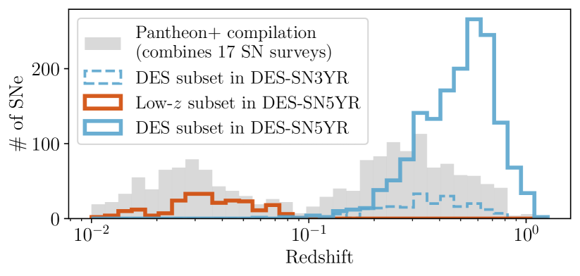
Figure 3: Histogram showing the redshift distribution of the DES-SN5YR sample, with new DES SNe in blue and our low-$z$ sample in red. For comparison the distribution of redshifts in the existing Pantheon+ sample is shown in grey (Brout et al., 2022a), which also includes the DES SNe from the DES-SN3YR analysis (blue dashed line). The five-year DES sample contains $\sim 4\times$ more supernovae above $z\sim 0.4$ than the Pantheon+ compilation.

We apply strict quality cuts to this sample of candidates to select our final high-quality sample for the Hubble diagram. The same quality cuts were applied to both the low-$z$ sample and the DES supernovae. First, we require a spectroscopic redshift of the host galaxy, good light-curve coverage (at least two detections with SNR$>5$ in two different bands), and a well converged light-curve fit using the SALT3 model (Kenworthy et al., 2021; Taylor et al., 2023); this reduces the DES sample size to 3621. Additional requirements include light-curve parameters (stretch and colour) within normal range for SNe Ia, a well constrained time of peak brightness, good SALT3 fit-probability, and valid distance-bias correction from our simulation (see Table 4 of Vincenzi et al., 2024, for more detail). Our final Hubble-diagram sample includes 1635 supernovae, of which 1499 have a machine-learning probability of being a Type Ia greater than 50% (see Sec. 2.2). Note that we do not perform a cut on this machine-learning probability, rather we use it in the BEAMS formalism that produces our Hubble diagram and to weight the SN distance uncertainties in the fits to the final Hubble diagram (Kessler et al., 2023). The set of all DES light curves is visualised in Fig. 2.

Since we focus on minimizing potential systematic errors, we only use the best-calibrated, most homogeneous sample of low-$z$ SNe Ia. To reduce the impact of peculiar velocity uncertainties we remove SNe with $z<0.025$. We furthermore combine only a subset of the available low-redshift samples: CfA3&4, CSP, and Foundation SNe, which are the four largest low-$z$ samples with the most well-understood photometric calibration. Our low-$z$ sample thus totals 194 SNe with $z<0.1$; this can be compared to Pantheon+, for which the low-$z$ sample was almost four times larger (741 SNe at $z<0.1$). We have thus exchanged the statistical constraining power of more low-$z$ SNe for better control of systematics. The redshift distribution of our sample compared to the compilation of historical samples in Pantheon+ is shown in Fig. 3. To conclude, the final DES-SN5YR sample includes 1635 DES SNe and 194 low-$z$ external SNe, for a total of 1829 SNe.

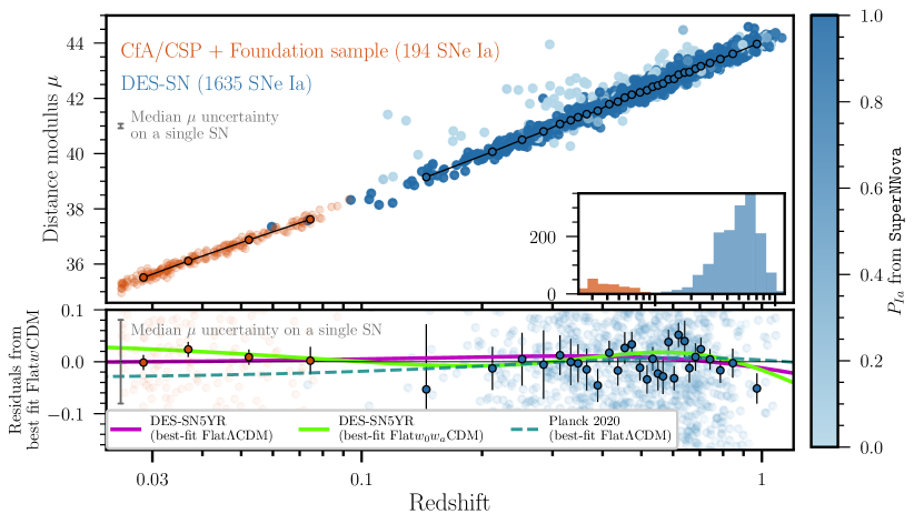
Figure 4: Hubble diagram of DES-SN5YR. We show both the single SN events and the redshift-binned SN distance moduli. Redshift bins are adjusted so that each bin has the same number of SNe ($\sim 50$). The 1635 new DES supernovae are in blue, and in the upper panel they are shaded by their probability of being a Type Ia; most outliers are likely contaminants (pale blue). The inset shows the number of SNe as a function of redshift (same $z$-range as the main plot). The lower panel shows the difference between the data and the best fit Flat-$w$CDM model from DES-SN5YR alone (third result in Table 2), and overplots three other best fit cosmological models — Flat-$\Lambda$CDM model from DES-SN5YR alone (magenta line, first result in Table 2), Flat-$w_{0}w_{a}$CDM model from DES-SN5YR alone (green line, fourth result in Table 2), and Planck 2020 Flat-$\Lambda$CDM model without SN data (dashed line, $\Omega_{\rm M}^{\rm Planck}=$$0.317\pm 0.008$).

2.2 From light curves to Hubble diagram

A critical step in the cosmology analysis is to convert each supernova’s light curve (magnitude vs time in multiple bands; see examples in Fig. 2) to a single calibrated number representing its standardized magnitude and estimated distance modulus.

To achieve this, we use the SALT3 light-curve fitting model as presented in Kenworthy et al. (2021); Taylor et al. (2023) and retrained in Vincenzi et al. (2024) to determine the light-curve fit parameters, amplitude of the SN flux ($x_{0}$), stretch ($x_{1}$), and color ($c$). These fitted parameters are used to estimate the distance modulus, $\mu\equiv m-M$, using an adaptation of the Tripp equation (Tripp, 1998) that includes a correction for observed correlations between SN Ia luminosity and host properties, ${\gamma}G_{\rm host}$. This correction has historically been described as a “mass step” but we also consider the possibility that it is a “color step” (see Sec. 2.2 of Vincenzi et al., 2024),

$$\mu_{{\rm obs},i}=m_{x,i}+\alpha x_{1,i}-\beta c_{i}+\gamma G_{{\rm host},i}-M-\Delta\mu_{{\rm bias},i},$$ (1)

where $m_{x}=-2.5\log_{10}(x_{0})$. The constants $\alpha$, $\beta$, and $\gamma$ are global parameters determined from the likelihood analysis of all the SNe on the Hubble diagram, while the terms subscripted by $i$ refer to parameters of individual SNe. We find $\alpha=0.161\pm 0.001$, $\beta=3.12\pm 0.03$, and $\gamma=0.038\pm 0.007$. We marginalize over the absolute magnitude $M$ (see Sect. 3). The final term in Eq. 1 accounts for selection effects, Malmquist bias, and light curve fitting bias.

The nuisance parameters and $\Delta\mu_{{\rm bias},i}$ term in Eq. 1 are determined using the “BEAMS with Bias Corrections” (BBC) framework (Kessler & Scolnic, 2017). In particular, bias corrections $\Delta\mu_{{\rm bias},i}$ are estimated from a large simulation of our sample. The simulation models the rest-frame SN Ia spectral energy distribution (SED) at all phases, SN correlations with host-galaxy properties, SED reddening through an expanding universe, broadband $griz$ fluxes, and instrumental noise (see Fig. 1 in Kessler et al., 2019a). Using Eq. 1 there remains intrinsic scatter of $\sim 0.1$ mag in Hubble residuals. Following the numerous recent studies on understanding and modelling SN Ia dust extinction and progenitors (Wiseman et al., 2021, 2022; Duarte et al., 2022; Dixon et al., 2022; Chen et al., 2022; Meldorf et al., 2023), we model this residual scatter using the dust-based model from Brout & Scolnic (2021); Popovic et al. (2023a), which improves on the previous commonly used models in Kessler et al. (2013) that are based on SALT2 error models in Guy et al. (2010); Chotard et al. (2011). This intrinsic scatter remains the largest source of systematic uncertainty from the simulation.

As we do not spectroscopically classify the SNe and thus expect contamination from core-collapse (CC) supernovae, we perform machine learning light-curve classification on the sample following Vincenzi et al. (2023); Möller et al. (2022). We implement two advanced machine learning classifiers, SuperNNova (Möller & de Boissière, 2020) and SCONE (Qu et al., 2021) and use state-of-the-art simulations to model contamination (estimated to be $\sim 6.5$%, see Table 10 and Sect. 7.1.5 of Vincenzi et al., 2024). Classifiers are trained using core-collapse and peculiar SN Ia simulations based on Vincenzi et al. (2021) and using state-of-the-art SED templates by Vincenzi et al. (2019); Kessler et al. (2019b). These DES simulations are the first to robustly reproduce the contamination observed in the Hubble residuals (Vincenzi et al., 2021, 2024, Table 10).

For each SN, the trained classifiers assign a probability of being a Type Ia, and these probabilities are included within the BEAMS framework to marginalize over core-collapse contamination and produce the final Hubble Diagram (Kunz et al., 2012; Hlozek et al., 2012). The final DES-SN5YR Hubble diagram is shown in Fig. 4 and includes 1829 SNe.

As discussed in Kessler et al. (2023); Vincenzi et al. (2024), the probability that each supernova is a Type Ia ($P_{\rm Ia}$) is incorporated in the BBC fit and used to calculate a BEAMS probability, $P_{{\rm B(Ia)}}$ (see Eq. 9 in Kessler et al., 2023). BEAMS probabilities are used to inflate distance uncertainties of likely contaminants by a factor $\propto 1/\sqrt{P_{{\rm B(Ia)}}}$ (see Eq. 10 in Vincenzi et al., 2024). Therefore, the released Hubble diagram data includes distance bias corrections and inflated distance uncertainties (see App. A), enabling users to fit the Hubble diagram without applying additional corrections. With this BEAMS uncertainty weight, we find 75 SNe with distance modulus uncertainties $\sigma_{\mu,i,\mathrm{final}}>1$ mag and 1331 SNe with $\sigma_{\mu,i,\mathrm{final}}<0.2$ mag.

Vincenzi et al. (2024) stops short of performing cosmological constraints but provides the corrected distance moduli $\mu$ along with their uncertainties $\sigma_{\mu}$, redshifts for each SN, and a statistical+systematic covariance matrix $C$, which we describe further in Sec. 3.

Armstrong et al. (2023) presents validation of the cosmological contours produced by our pipeline. Validation that our analysis pipeline is insensitive to the cosmological model assumed in our bias correction simulation appears in Camilleri et al. (in prep. 2024).

Cosmological Model	Friedmann Equation: $\mathbf{E(z)=H(z)/H_{0}=}$	Fit Parameters $\Theta$
Flat-$\Lambda$CDM	$\left[\Omega_{\rm M}(1+z)^{3}+(1-\Omega_{\rm M})\right]^{1/2}$	$\Omega_{\rm M}$
$\Lambda$CDM	$\left[\Omega_{\rm M}(1+z)^{3}+\Omega_{\rm\Lambda}+(1-\Omega_{\rm M}-\Omega_{\rm\Lambda})(1+z)^{2}\right]^{1/2}$	$\Omega_{\rm M},\Omega_{\rm\Lambda}$
Flat-$w$CDM	$\left[\Omega_{\rm M}(1+z)^{3}+(1-\Omega_{\rm M})(1+z)^{3(1+w)}\right]^{1/2}$	$\Omega_{\rm M},w$
Flat-$w_{0}$$w_{a}$CDM	$\left[\Omega_{\rm M}(1+z)^{3}+(1-\Omega_{\rm M})(1+z)^{3(1+w_{0}+w_{a})}e^{-3w_{a}z/(1+z)}\right]^{1/2}$	$\Omega_{\rm M},w_{0},w_{a}$

Table 1: Variations on the standard cosmological model that are tested in this paper, their Friedmann Equations, and the free parameters in the fit.

2.3 Unblinding criteria

Throughout our analysis, cosmological parameters estimated from real data were blinded. We validate our entire pipeline on detailed catalogue-level simulations and examine the cosmological parameters estimated from simulations to test that the input cosmology is recovered. In addition to the many tests described in Vincenzi et al. (2024), the final unblinding criteria that our data passed were:

• Accuracy of simulations: Reduced $\chi^{2}$ between the distribution of data and simulations across a variety of observables (redshift, SALT3 parameters and goodness of the fit, maximum signal-to-noise ratio at peak, host stellar mass) is required to be between 0.7 and 3.0 (see Vincenzi et al., 2024, Fig. 3-4).

• Pipeline validation using DES simulations: Demonstrate that our pipeline recovers the input cosmology. We produce 25 data-size simulated samples (statistically independent) assuming a Flat-$\Lambda$CDM universe with best-fit Planck value of $\Omega_{\rm M}$ and analyze them the same way as real data. We fit each Hubble diagram assuming a Flat-$w$CDM model with a Planck prior and find a mean bias of $w-w_{\rm true}\simeq 0.001\pm 0.020$, where $w$ is the mean value of the marginalized posterior of the dark energy equation of state parameter over the 25 samples, and $w_{\rm true}=-1$ is the model value of that parameter input to the simulation.

• Validation of contours: ensuring that our uncertainty limits accurately represent the likelihood of the models (Armstrong et al., 2023).

• Independence of reference cosmology: ensuring that our results are sufficiently independent of cosmological assumptions that enter our bias correction simulations (Camilleri et al., in prep. 2024).

2.4 Combining SN with other cosmological probes

We combine the DES-SN5YR cosmological constraints with measurements from other complementary cosmological probes. In particular, we use:

• Cosmic Microwave Background (CMB) measurements of the temperature and polarisation power spectra (TTTEEE) presented by the Planck Collaboration (2020). We use the Python implementation of Planck’s 2015 Plik_lite (Prince & Dunkley, 2019).

• Weak lensing and galaxy clustering measurements from the DES3$\times$2pt year-3 magnitude-limited (MagLim) lens sample; $3\times 2$-point refers to the simultaneous fit of three 2-point correlation functions, namely galaxy-galaxy, galaxy-lensing, and lensing-lensing correlations (Dark Energy Survey Collaboration, 2022, 2023).

• Baryon acoustic oscillation (BAO) measurements as presented in the extended Baryon Oscillation Spectroscopic Survey paper (eBOSS; Dawson et al., 2016; Alam et al., 2021), which adds the BAO results from SDSS-IV (Blanton et al., 2017) to earlier SDSS BAO data. Specifically, we use “BAO” to refer to the BAO-only measurements from the Main Galaxy Sample (Ross et al., 2015), BOSS (SDSS-III Alam et al., 2017), eBOSS LRG (Bautista et al., 2021), eBOSS ELG (de Mattia et al., 2021), eBOSS QSO (Hou et al., 2021), and eBOSS Lya (du Mas des Bourboux et al., 2020).

When combining these data we run simultaneous MCMC fits of the relevant data vectors. We present three combinations: the simplest CMB-dependent combination CMB+SN, a CMB-independent combination BAO+3$\times$2pt+SN, and a combination of them all.

3 Models and theory

We present cosmological results for the standard cosmological model – flat space with cold dark matter and a cosmological constant (Flat-$\Lambda$CDM) – and some basic extensions, such as relaxing the assumption of spatial flatness ($\Lambda$CDM), allowing for constant equation of state parameter ($w$) of dark energy (Flat-$w$CDM), and including a linear parameterisation for time-varying dark energy (Flat-$w_{0}w_{a}$CDM) in which the equation of state parameter is given by $w=w_{0}+w_{a}(1-a)$ (Chevallier & Polarski, 2001; Linder, 2003).

To calculate the theoretical distance as a function of redshift we begin with the comoving distance,

$$R_{0}\chi(\bar{z})=\frac{c}{H_{0}}\int_{0}^{\bar{z}}\frac{dz}{E(z)},$$ (2)

where $\bar{z}$ is the redshift due to the expansion of the Universe, $E(z)\equiv H(z)/H_{0}$ is the normalized redshift-dependent expansion rate and is given for each cosmological model by the expression in Table 1, $R_{0}=c/(H_{0}\sqrt{|\Omega_{\rm K}|})$ is the scale factor with dimensions of distance (where subscript $0$ indicates its value at the present day), and $\Omega_{\rm K}\equiv 1-\Omega_{\rm M}-\Omega_{\rm\Lambda}$ is the curvature term. The dimensionless scale factor ($a\equiv R/R_{0}$) at the time of emission for an object with cosmological redshift $\bar{z}$ is $a=1/(1+\bar{z})$. The luminosity distance is given by,

$$D_{\rm L}(z_{\rm obs},\bar{z})=(1+z_{\rm obs})R_{0}S_{k}(\chi(\bar{z})),$$ (3)

where $z_{\rm obs}$ is the observed redshift, and the curvature is captured by $S_{k}(\chi)=\sin\chi$, $\chi$, and $\sinh\chi$ for closed ($\Omega_{\rm K}<0$), flat ($\Omega_{\rm K}=0$), and open ($\Omega_{\rm K}>0$) universes respectively.

To compare data (Eq. 1) to theory we calculate the theoretical distance modulus, which is dependent on the set of cosmological parameters we are interested in ($\Theta$, given in the right column of Table 1),

$$\mu(z,\Theta)=5\log_{10}(D_{\rm L}(z,\Theta)/1~{}{\rm Mpc})+25.$$ (4)

We compute the difference between data and theory for every $i$th supernova, $\Delta\mu_{i}=\mu_{{\rm obs},i}-\mu(z_{i},\Theta)$, and find the minimum of

$$\chi^{2}=\Delta\mu_{i}\mathcal{C}_{ij}^{-1}\Delta\mu_{j}^{T}~{},$$ (5)

where $\mathcal{C}^{-1}$ is the inverse covariance matrix (including both statistical and systematic errors) of the $\Delta\mu$ vector (see Sec. 3.6 of Vincenzi et al., 2024).

The uncertainty covariance matrix includes a diagonal statistical term (discussed Sec. 2.2) and a systematic term. The systematic covariance matrix is built following the approach in Conley et al. (2011) and accounts for systematics such as calibration, intrinsic scatter, and redshift corrections (see Table 6 of Vincenzi et al., 2024). Each element of the covariance matrix expresses the covariance between two of the SNe in the sample. The covariance matrix has dimensions of the number of supernovae $N_{\rm SNe}\times N_{\rm SNe}$ and we follow the formalism introduced by Brout et al. (2021) and Kessler et al. (2023).

Finally, the absolute magnitude of SNe Ia ($M$) and the $H_{0}$ parameter (which appears in the luminosity distance) are completely degenerate and therefore they are combined in the single parameter $\mathcal{M}=M+5\log_{10}(c/H_{0})$. All of our cosmology results are marginalized over this term. Therefore, the value of $H_{0}$ has no impact on the fitting of our cosmological results, and we do not constrain $H_{0}$. While $\mathcal{M}$ has no impact on cosmology fitting, a precise value is needed to simulate bias corrections. The $\mathcal{M}$ uncertainty is below 0.01, resulting in a negligible impact on bias corrections (Brout et al., 2022a; Camilleri et al., in prep. 2024).

4 Results

With the new DES high-redshift supernova sample we can put strong constraints on cosmological models. Of particular interest is whether dark energy is consistent with a cosmological constant or whether its density and/or equation of state parameter varies over the wide redshift range of our sample. The results of our cosmological fits are outlined in this section and summarized in Table 2, and their implications are explored in Sec. 5.

We estimate cosmological constraints using the CosmoSIS framework (Zuntz et al., 2015), the samplers emcee for best fits (Foreman-Mackey et al., 2013), and PolyChord for tension metrics (Handley et al., 2015), except for fits that include BAO+3$\times$2pt, which are calculated using PolyChord for both best fit and tensions. For all fits we present the median of the marginalized posterior and cumulative 68.27% confidence intervals. The chains and code (with the flexibility to test other statistical choices) will be made available on github upon acceptance of this paper. Figs. 5, 6, 7 and 8 all present the joint probability contours for 68.3% and 95.5%.

4.1 Constraints on Cosmological Parameters

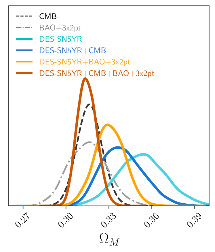
Figure 5: Constraints on matter density in the Flat-$\Lambda$CDM model from DES-SN5YR only (cyan), DES-SN5YR combined with CMB constraints from Planck Collaboration (2020) (blue), and DES-SN5YR combined with BAO+3$\times$2pt (orange), and all probes combined (DES-SN5YR+BAO+3$\times$2pt and CMB constraints, dark orange). CMB constraints only and BAO+3$\times$2pt constraints alone are also shown for comparison (dashed and dotted-dashed respectively).

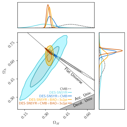
Figure 6: Constraints for $\Lambda$CDM model (non-zero curvature allowed) from the DES-SN5YR dataset only (cyan), from DES-SN5YR combined with BAO and weak lensing measurements (orange), and from DES-SN5YR combined with CMB measurements (blue). For comparison, we also present cosmological constraints from Planck Collaboration (2020) only (black dashed).

4.1.1 Flat-$\Lambda$CDM

For the simplest parameterization, Flat-$\Lambda$CDM, $\Omega_{\rm M}$ is the only free parameter. We show the probability density function (PDF) of this constraint for DES-SN5YR in Fig. 5; we measure a value of $\Omega_{\rm M}=$$0.352\pm 0.017$. We also show the probability distribution of the Planck Collaboration (2020) measurement of $\Omega_{\rm M}^{\rm Planck}=$$0.317\pm 0.008$. These are approximately $2\sigma$ apart, but not in significant tension as discussed in Sec 4.2.

Combining DES-SN5YR with Planck CMB gives $\Omega_{\rm M}=$$0.338^{+0.016}_{-0.014}$, while combining with BAO+3$\times$2pt gives $\Omega_{\rm M}=$$0.330^{+0.011}_{-0.010}$. Combining all three gives $\Omega_{\rm M}=$$0.315\pm 0.007$. Interestingly, the combination of all data sets (dark orange in Fig. 5) gives a lower $\Omega_{\rm M}$ than any of the other combinations. The reason can be seen in Fig. 6, where all constraints cross the Flat Universe line to the upper left of any individual best fit.

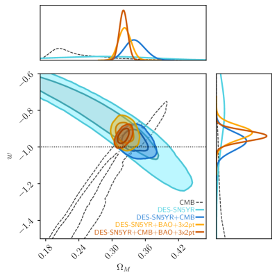
Figure 7: Same as Fig. 6 but for Flat $w$CDM model. The horizontal dotted line marks the equation of state values for a cosmological constant, i.e. $w=-1$.

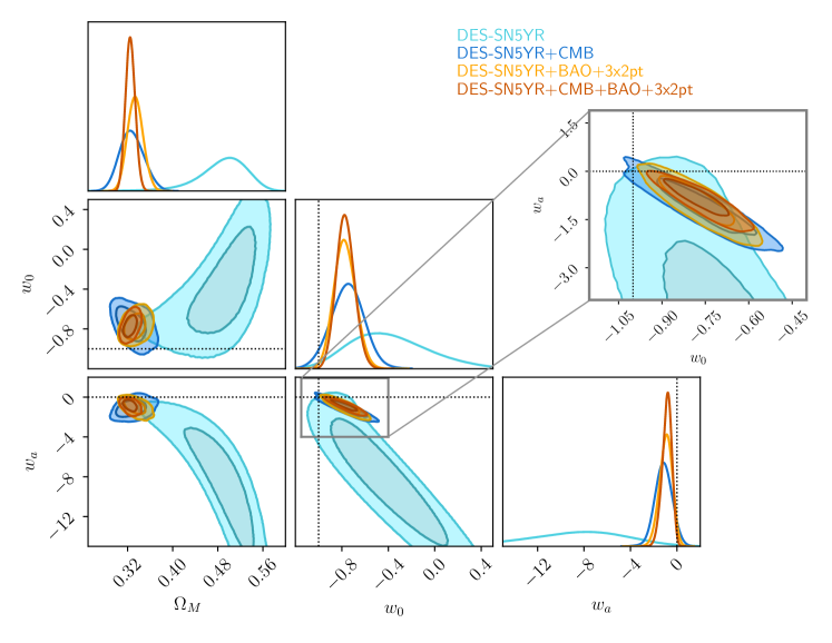
Figure 8: Same as Fig. 6 but for $w_{0}w_{a}$CDM model. The dashed crosshairs mark the equation of state values for a cosmological constant, i.e. $(w_{0},w_{a})=(-1,0)$. The residuals between the DES-SN5YR best fit Flat-$w_{0}w_{a}$CDM w.r.t. Flat-$w$CDM model are presented in Fig. 4.

4.1.2 $\Lambda$CDM

Fitting DES-SN5YR to the $\Lambda$CDM model, we find $(\Omega_{\rm M},\Omega_{\rm\Lambda})$=($0.291^{+0.063}_{-0.065}$, $0.55\pm 0.17$), consistent with a flat universe ($\Omega_{\rm K}$=$0.16\pm 0.16$); see Fig. 6. Combining DES-SN5YR with BAO+3$\times$2pt is also consistent with a flat Universe, with uncertainties on $\Omega_{\rm K}$ reduced to $\sim\pm 0.034$, while the combination with Planck gives $\Omega_{\rm K}=$$0.010\pm 0.005$. The combination of all three gives $\Omega_{\rm K}=$$0.002^{+0.004}_{-0.003}$.

4.1.3 Flat-$w$CDM

Fitting DES-SN5YR to the Flat-$w$CDM model, we measure $(\Omega_{\rm M},w)=($$0.264^{+0.074}_{-0.096}$,$-0.80^{+0.14}_{-0.16}$$)$; see Fig. 7. This is consistent with a cosmological constant (within $2\sigma$), although our data favors a $w$-value that is slightly larger than $-1$.

The $w-\Omega_{\rm M}$ contours from SN alone are highly non-Gaussian with a curved ‘banana’-shaped degeneracy. The best fit value for $w$ or $\Omega_{\rm M}$ is thus an insufficient summary of the SN information, as a small shift along the degeneracy direction can result in large shifts in the best-fit values. To address this issue, in Camilleri et al. (in prep. 2024) we introduce a new parameter, $Q_{H}(z)\equiv-\ddot{a}/(aH_{0}^{2})\equiv q(H/H_{0})^{2}$. This combination of the deceleration parameter $q$ and the Friedmann equation $H/H_{0}$ follows the curve of the degeneracy in the $w-\Omega_{\rm M}$ plane. Therefore, measuring $Q_{H}(z)$ summarizes the supernova information in a single, almost degeneracy-free value. One has to choose the redshift at which one quotes $Q_{H}(z)$, to best match the angle of the degeneracy for the redshift range of the sample. We find $Q_{H}(z=0.2)=-0.340\pm 0.032$ using DES-SN5YR only (see Camilleri et al., in prep. 2024). This $Q_{H}$ value can be used to roughly approximate the DES-SN5YR results and characterize the constraining power without the need for a full fit to the Hubble diagram.

The degeneracy in the $w-\Omega_{\rm M}$ plane is broken by combining SNe with external probes. Combining with Planck, we measure $(\Omega_{\rm M},w)=($$0.337^{+0.013}_{-0.011}$,$-0.955^{+0.032}_{-0.037}$$)$, again within 2$\sigma$ of a cosmological constant. Planck alone provides only a loose constraint on the equation of state parameter of dark energy, $w^{\rm Planck}=-1.51^{+0.27}_{-0.18}$; combining with DES-SN5YR reduces the uncertainty significantly due to the different degeneracy direction, demonstrating the combined constraining power of these two complementary probes.

Combining DES-SN5YR with BAO+3$\times$2pt we find $w=$$-0.922^{+0.035}_{-0.037}$, slightly over $2\sigma$ from the cosmological constant. This data combination demonstrates that these late-universe probes alone provide constraints that are consistent with – and of comparable constraining power to – the combination of SN and CMB data. The full combination of all data sets gives $w=$$-0.941\pm 0.026$.

4.1.4 Flat-$w_{0}w_{a}$CDM

Fitting DES-SN5YR alone to the Flat-$w_{0}w_{a}$CDM model gives an equation of state that is slightly over $2\sigma$ from a cosmological constant, marginally preferring a time-varying dark energy $(\Omega_{\rm M},w_{0},w_{a})=$($0.495^{+0.033}_{-0.043}$, $-0.36^{+0.36}_{-0.30}$, $-8.8^{+3.7}_{-4.5}$$)$; see Fig. 8.

Combining DES-SN5YR and the CMB, we find $(\Omega_{\rm M},w_{0},w_{a})=$($0.325^{+0.016}_{-0.012}$,$-0.73\pm 0.11$,$-1.17^{+0.55}_{-0.62}$), which again deviates slightly from the cosmological constant. The same trend is seen when combining with BAO+3$\times$2pt and with all data combined. The negative $w_{a}$ means that the dark energy equation of state parameter is increasing with time (sometimes referred to as a “thawing” model).

Table 2: Results for four different cosmological models, sorted into sections for different combinations of observational constraints. These are the medians of the marginalized posterior with 68.27% integrated uncertainties (‘cumulative’ option in ChainConsumer). For each fit we also show the $\chi^{2}$ per degree of freedom as a measure of the goodness of fit.

	$\Omega_{\rm M}$	$\Omega_{\rm K}$	$w_{0}$	$w_{a}$	$\chi^{2}/{\rm dof}$
DES-SN5YR (no external priors)
Flat-$\Lambda$CDM	$0.352\pm 0.017$	-	-	-	1649/1734=0.951
$\Lambda$CDM	$0.291^{+0.063}_{-0.065}$	$0.16\pm 0.16$	-	-	1648/1733=0.951
Flat-$w$CDM	$0.264^{+0.074}_{-0.096}$	-	$-0.80^{+0.14}_{-0.16}$	-	1648/1733=0.951
Flat-$w_{0}w_{a}$CDM	$0.495^{+0.033}_{-0.043}$	-	$-0.36^{+0.36}_{-0.30}$	$-8.8^{+3.7}_{-4.5}$	1641/1732=0.948
DES-SN5YR + Planck 2020
Flat-$\Lambda$CDM	$0.338^{+0.016}_{-0.014}$	-	-	-	2237/2349=0.952
$\Lambda$CDM	$0.359^{+0.014}_{-0.016}$	$0.010\pm 0.005$	-	-	2231/2348=0.950
Flat-$w$CDM	$0.337^{+0.013}_{-0.011}$	-	$-0.955^{+0.032}_{-0.037}$	-	2234/2348=0.951
Flat-$w_{0}w_{a}$CDM	$0.325^{+0.016}_{-0.012}$	-	$-0.73\pm 0.11$	$-1.17^{+0.55}_{-0.62}$	2231/2347=0.951
DES-SN5YR + SDSS BAO and DES Y3 3$\times$2pt
Flat-$\Lambda$CDM	$0.330^{+0.011}_{-0.010}$	-	-	-	2194/2212=0.992
$\Lambda$CDM	$0.327^{+0.012}_{-0.011}$	$0.030\pm 0.034$	-	-	2194/2211=0.992
Flat-$w$CDM	$0.323^{+0.011}_{-0.010}$	-	$-0.922^{+0.035}_{-0.037}$	-	2188/2211=0.989
Flat-$w_{0}w_{a}$CDM	$0.334\pm 0.012$	-	$-0.778^{+0.088}_{-0.080}$	$-0.93^{+0.46}_{-0.53}$	2191/2210=0.992
DES-SN5YR + Planck 2020 + SDSS BAO and DES Y3 3$\times$2pt
Flat-$\Lambda$CDM	$0.315\pm 0.007$	-	-	-	2791/2828=0.987
$\Lambda$CDM	$0.318^{+0.011}_{-0.010}$	$0.002^{+0.004}_{-0.003}$	-	-	2825/2827=0.999
Flat-$w$CDM	$0.321\pm 0.007$	-	$-0.941\pm 0.026$	-	2785/2827=0.985
Flat-$w_{0}w_{a}$CDM	$0.325\pm 0.008$	-	$-0.773^{+0.075}_{-0.067}$	$-0.83^{+0.33}_{-0.42}$	2782/2826=0.984

4.2 Goodness of fit and tension

4.2.1 $\chi^{2}$ per degree of freedom

To assess whether our best fits are good fits we calculate the $\chi^{2}$ per degree of freedom for all our dataset and model combinations; see the last column of Table 2. The $\chi^{2}$ we use for this test is the maximum likelihood of the entire parameter space, not the marginalized best fit for each parameter.

The number of degrees of freedom is the number of data points minus the number of parameters that are common to all datasets (i.e., the cosmological parameters of interest). The number of data points added by the CMB, BAO, and 3$\times$2pt is respectively 615, 8, and 471. Due to our treatment of contamination (by inflating the uncertainties of SNe with a low $P_{\rm Ia}$), we approximate the effective number of data points in the DES-SN5YR sample by $\sum P_{{\rm B(Ia)}}=1735$ (rather than the total number of data points, 1829).

Ideally, a good fit should have $\chi^{2}/$d.o.f.$\sim 1.0$. The slightly low $\chi^{2}/$d.o.f. for the DES-SN5YR data arises because $\sum P_{{\rm B(Ia)}}$ only approximates the number of degrees of freedom, and the same behaviour is also seen in simulations.

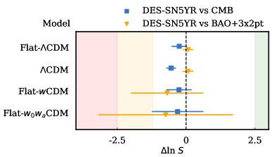
Figure 9: Measurements of Suspiciousness $(\Delta\ln(S))$ between the DES-SN5YR and Planck 2020 datasets for the four models constrained in this paper. Further left indicates higher tension where the shaded regions reflect “substantial” (yellow) and “strong” (red) evidence of tension according to Jeffreys’ scale (Jeffreys, 1961). The values and uncertainties represent the mean and standard deviation of realizations estimating sample variance using the ANESTHETIC software.

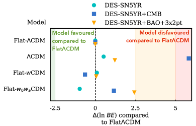
Figure 10: Bayesian Evidence difference relative to Flat-$\Lambda$CDM ($\Delta$(ln $BE$)). We present the results for the four different models tested in this analysis and for the three combination of datasets used (DES only in cyan, DES+Planck in blue, DES+BAO+3$\times$2pt in orange). An increase (decrease) in $\Delta$(ln $BE$) indicates that a model is disfavoured (favoured) compared to Flat-$\Lambda$CDM.

4.2.2 Suspiciousness

Suspiciousness, $S$, (Handley & Lemos, 2019) is closely related to the Bayes ratio, $R$, and can be used to assess whether different datasets are consistent. However, while the Bayes ratio has been shown to be prior-dependent (Handley & Lemos, 2019), with wider prior widths boosting the confidence, Suspiciousness is prior independent. Therefore, Suspiciousness is ideal for cases such as ours where we have chosen deliberately wide and uninformative priors (Lemos et al., 2021, Sec. 4.2). Jeffreys’ scale (Jeffreys, 1961) suggests $\ln S<-2.5$ is “strong” tension, $-2.5<\ln~{}S<-1.2$ is “substantial” tension, and $\ln S>-1.2$ indicates the datasets are in agreement.

We determine $\ln S$ using the ANESTHETIC software (Handley, 2019), which produces an ensemble of realizations used to estimate sample variance. Results are quoted using the mean of the ensemble, with the error bars reflecting the standard deviation.

In Fig. 9 we plot the Suspiciousness values for the DES-SN5YR data vs Planck 2020 and vs BAO+3$\times$2pt data. We find no indication of tension using any of the four models investigated in this paper.

4.3 Model Selection

Finally, we use Bayesian Evidence to test whether the extra parameters in the more complex models we test are warranted, given the data. In Fig. 10, we present the difference in the logarithm of the Bayesian Evidence, $\Delta$(ln $BE$), relative to Flat-$\Lambda$CDM for the four different models tested in this analysis and for the three combinations of datasets used in Fig. 10.

To evaluate the strength of evidence when comparing Flat-$\Lambda$CDM with more complex models, we again use Jeffreys’ scale. This empirical scale suggests that $\Delta$(ln $BE$)$>2.5$ (and $<-2.5$) is moderate evidence against (in support of) the more complex model, whereas $\Delta$(ln $BE$)$>5$ (and $<-5$) is strong evidence against (in support of) the more complex model (for a review of model selection in cosmology see Trotta, 2008). We note that none of the datasets considered in this analysis strongly favours cosmological models beyond Flat-$\Lambda$CDM. The priors that we choose for model comparison are $w\in(-1.5,-0.5)$, $w_{a}\in(-10,10)$ and $\Omega_{\rm K}\in(-0.5,0.5)$. We consider these priors (which determine the penalty for more complex models) to be reasonable in terms of general considerations, such as avoiding universes that are younger than generally accepted stellar ages (see Section 5.1.3). We also find the results to be consistent with the Akaike Information Criteria, another commonly used model comparator.

5 Discussion

5.1 The big questions

5.1.1 Is the expansion of the Universe accelerating?

Twenty five years ago Riess et al. (1998) found 99.5%–99.9% ($2.8\sigma$ to $3.9\sigma$) evidence for an accelerating Universe, by considering the deceleration parameter $q\equiv(a\ddot{a})\dot{a}^{-2}$ and integrating over the likelihood that $q_{0}<0$. Importantly they note that since $q_{0}$ is measured at the present day but the data span a wide range of redshifts, $q_{0}$ can only be measured within the context of a model, either cosmographic or physically motivated. They used the $\Lambda$CDM model, in which $q_{0}=\Omega_{\rm M}/2-\Omega_{\rm\Lambda}$.

Doing the same with DES-SN5YR data gives 99.99998% confidence ($5.2\sigma$) that $q_{0}<0$ in $\Lambda$CDM, or a $2\times 10^{-7}$ chance that the expansion of the Universe is not accelerating. As noted in Section 4.1.3, our confidence is even higher that the universe was accelerating at $z\sim 0.2$. When we further assume flatness, the confidence in an accelerating Universe is overwhelming (no measurable likelihood for a decelerating Universe) and we find $q_{0}=$$-0.530^{+0.018}_{-0.017}$. For more fits of $q_{0}$ using a cosmographic approach see Camilleri et al. (in prep. 2024).

5.1.2 Is dark energy a cosmological constant?

As seen in Sec 4.1, a cosmological constant is a good fit to our data, but not the best fit. Our best fit equation of state parameter is slightly (more than $1\sigma$) higher than the cosmological constant value of $w=-1$ (both for SNe alone and in combination with Planck or BAO+3$\times$2pt). Our result agrees with the recent result from the UNION3 compilation analyzed with the UNITY framework (Rubin et al., 2023) (which appeared while this paper was under internal review). The Pantheon$+$ result (Brout et al., 2022a) is within $1\sigma$ of $w=-1$, but also on the high side ($w=-0.90\pm 0.14$).

Furthermore, our analysis slightly prefers a time-varying dark energy equation of state parameter when we fit for $w(a)$ such that the equation of state parameter increases with time (again for all data combinations), known as a “thawing” model. Model selection, however, is inconclusive.

The constraints on time-varying $w$ are enabled by the wide redshift range of the DES-SN5YR sample. Our analysis as described in Vincenzi et al. (2024) gives us confidence that systematic uncertainties in this data are below the level of our statistical precision. Nevertheless, it is important to recognize that (a) the low-$z$ sample is the one for which we have the least systematic control and (b) the very high-redshift SNe are the ones for which bias-corrections are large ($>0.1$ mag) and more uncertain (e.g., accurate estimation of spectroscopic redshift efficiency is more challenging as we go to higher redshifts), and for which the uncertainties on the rest-frame UV part of the SN Ia spectral energy distribution have more impact on SN distances estimations (see also Brout et al., 2022a).

To test whether our fits are dominated by any particular redshift range we ran cosmological fits (a) removing low-$z$ data (i.e., DES SNe alone) and (b) removing high-$z$ data (i.e., removing $\sim 80$ SNe at $z>0.85$, for which we use only two bands; see Fig. 2). Most of the cosmological results obtained with the subsamples are consistent with the results found for the full sample, (based on running the same test on 25 simulated data samples). However, we found that removing the low-$z$ sample shifts the contours in the Flat-$w$CDM slightly down, which would make the combined fits more consistent with $w=-1$. The Flat-$w_{0}w_{a}$CDM results are stable to sub-sample selection.

We showed in Vincenzi et al. (2024) that systematic uncertainties are sub-dominant to the statistical uncertainties in our sample. Nevertheless, in the future a new low-redshift sample (see Sec. 5.3) would help alleviate any remaining doubt about calibration and systematics in the existing low-$z$ sample, and an even higher-redshift supernova survey would help alleviate any modelling concerns by minimizing selection effects even at $z\sim 1$.

5.1.3 How old is the Universe?

One of the issues that the discovery of dark energy solved is the age of the Universe ($t_{0}$) problem – globular cluster age estimates, in combination with high estimates of $H_{0}$, were inconsistent with models that were not accelerating (VandenBerg et al., 1996; Gratton et al., 1997; Chaboyer et al., 1998).

Our results, which favor a dark energy equation of state parameter slightly higher than $w=-1$ would imply that the age is slightly younger than the age found in a Universe where dark energy is a cosmological constant (for the same values of $H_{0}$ and present dark energy density).

To calculate the Universe’s age, one needs a value of $H_{0}$ in addition to the best fit cosmological model. Since we do not constrain $H_{0}$ in this analysis, we present our measurement of the combination $H_{0}t_{0}$. In other words, we give $t_{0}$ in units of the Hubble time $t_{H}\equiv 1/H_{0}$. Our best-fit DES-SN5YR result in Flat-$\Lambda$CDM would have an age of $(0.921\pm 0.013)t_{H}$. This is $\sim 3$% younger than Planck ($t_{\rm age}^{\rm Planck}=(0.950\pm 0.007)t_{H}$), corresponding to an age difference of approximately $-0.4$ Gyr. Our best fit Flat-$w_{0}w_{a}$CDM model gives an age $(0.86\pm 0.02)t_{H}$, about 9% younger than the Flat-$\Lambda$CDM Planck result, corresponding to an age difference of approximately $-1.3$ Gyr. Such a young age is unlikely given the age of the oldest globular clusters (Valcin et al., 2020; Cimatti & Moresco, 2023; Ying et al., 2023). In the future, this information could be used as a prior to limit the feasible range of time-varying dark energy.

5.1.4 Does our best fit resolve the Hubble tension?

As pointed out in Planck Collaboration (2020, their Sec. 5.4), the only basic extensions to the base Flat-$\Lambda$CDM model that resolve the $H_{0}$ tension are those in which the dark energy equation of state is allowed to vary away from $w=-1$. In the $w$CDM model a phantom equation of state parameter of $w\sim-1.5$ would help resolve the tension (Di Valentino et al., 2021, their Sec. 5.1), and it is clear from Fig. 7 that CMB alone actually prefers $w<-1$. In this model, Planck alone does not constrain $H_{0}$ very tightly, and they refrain from quoting a value, (see Table 5 of Planck Collaboration (2020)), but lower $w$ correlates with higher $H_{0}$. However, the DES-SN5YR data shows a slight tendency for $w>-1$, essentially ruling out this solution within $w$CDM.

5.2 Comparison with DES-SN3YR and Pantheon+

It is informative to compare the results of the previous DES-SN3YR analysis (Dark Energy Survey Collaboration, 2019; Brout et al., 2019a) with the results of the DES-SN5YR analysis presented in this work. The DES-SN3YR analysis included 207 spectroscopically confirmed SNe Ia from DES and 127 low-redshift SNe from CfA and CSP samples (see also Fig. 3). A fraction of those events is in common between both analyses (55 from low-$z$ external samples and 146 DES SNe).

However, the DES-SN3YR analysis differs from the analysis presented here in many aspects. The SN Ia intrinsic scatter modelling has been significantly improved (from ‘G10’ and constant $\sigma_{\rm int}$ floor, to the more sophisticated modelling of intrinsic scatter introduced by Brout & Scolnic, 2021; Popovic et al., 2023a), the BBC software has been updated (from BBC ‘5D’ and a binned approach, to BBC ‘4D’ and an unbinned approach), the $x_{1}-M_{\star}$ correlations have been incorporated into simulations (following the work by Smith et al., 2020b; Popovic et al., 2021), and the light-curve fitting model has been updated from the SALT2 model to the SALT3 model (see Taylor et al., 2023, for a comparison between SALT2 and SALT3 using the DES-SN3YR sample). Finally, the DES-SN3YR analysis did not require machine-learning classification and the implementation of the BEAMS approach because it is a sample of spectroscopically selected SNe Ia. We compare the final SN distances in Fig. 11 and find consistent results (differences in binned distances are on average 0.02 mag, even in the redshift ranges where contamination is expected to be high). The cosmological results from DES-SN3YR and DES-SN5YR are consistent within uncertainties (when assuming Flat-$\Lambda$CDM, $\Omega_{\rm M}$ are $0.331\pm 0.038$ and $0.352\pm 0.017$ for DES-SN3YR and DES-SN5YR respectively, while when assuming Flat-$w$CDM and including CMB priors, $w$ are $-0.978\pm 0.059$ and $-0.955^{+0.032}_{-0.037}$).

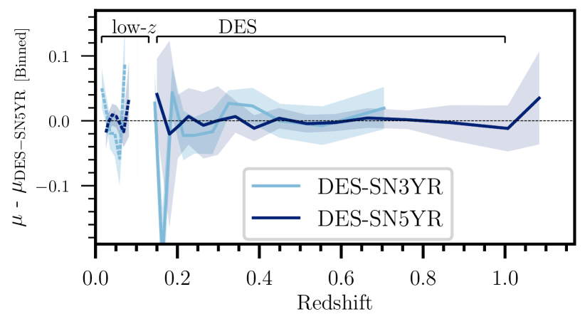
Figure 11: Comparison between Hubble residuals for the DES-SN3YR and DES-SN5YR analyses w.r.t. the best fit Flat-$w$CDM for the DES-SN5YR analysis. Hubble residuals are binned in redshift and we present the weighted mean and standard deviation of the mean in each redshift bin. The redshift range covered by the low-$z$ sample is highlighted and shown with thick dotted lines. The two DES samples are consistent with each other. Note the DES-SN3YR analysis only includes spectroscopically confirmed SNe whereas the DES sample in the DES-SN5YR analysis consists entirely of photometrically identified SNe Ia and extends to higher-$z$.

The other main dataset we can compare to is Pantheon+, which contains a significant amount of independent data (all the high-$z$ data). The DES sample is on average much higher redshift than the Pantheon+ sample (see Fig. 3), with over a quarter of the DES-SN5YR sample being at high enough redshift ($z\gtrsim 0.64$) to probe the likely decelerating period of the Universe (compared to 6% in Pantheon+). We show a comparison of the contours in Fig. 12. We find very similar constraining power between Pantheon+ and DES-SN5YR, and the DES-SN5YR value of $w$ is within $1\sigma$ of Pantheon+ (Brout et al., 2022a). These analyses are not fully independent as a fraction of the low-$z$ sample is shared. However, all of the high-$z$ dataset is independent, and DES is a photometric sample while Pantheon+ is fully spectroscopic. The constraints on $w$ are similar between DES and Pantheon+ as DES high-$z$ has better precision per SN than Pantheon+ and has significantly higher statistical power at $z>0.4$ (see Fig. 3), but Pantheon+ used $2\times$ more low-redshift SNe (which we do not include in order to be able to better control systematic uncertainties).

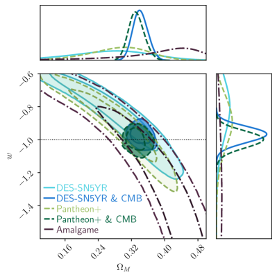
Figure 12: Constraints in Flat-$w$CDM from the DES-SN5YR sample, the Pantheon+ sample (with and without CMB priors), and the Amalgame sample. The constraining power of the DES-SN5YR and Pantheon+ samples is comparable and consistent, despite Pantheon+ being a spectroscopic SN Ia sample combining 17 different surveys. The “Amalgame” sample includes the SDSS and PS1 photometric SN samples ($>1700$ intermediate-redshift and high-redshift SNe), however it does not include a low-$z$ anchoring sample (hence the larger contours). DES-SN5YR and Pantheon+ are also combined with CMB constraints (for both we use the Planck lite Python implementation presented by Prince & Dunkley, 2019). The horizontal dotted line marks the equation of state values for a cosmological constant.

5.3 DES and Next Generation Supernova Samples

This analysis has shown that moving from a spectroscopically confirmed sample as done in Dark Energy Survey Collaboration (2019) to a photometric sample can increase the sample size of well-measured supernovae significantly (from 207 DES SNe Ia in DES-SN3YR to $>1600$ in DES-5YR), consistent with an analysis of Pan-STARRS SNe in Jones et al. (2018). This improvement arises because photometric classification alleviates the bottleneck of limited spectroscopic resources. The improvement will increase for future surveys as more candidates are discovered, but the available time for spectroscopy does not increase commensurately. Importantly, the work of Vincenzi et al. (2024) shows that systematic uncertainties due to photometric classification are not limiting. Instead, the “conventional” systematics of calibration and modeling the intrinsic scatter remain the most significant challenges.

There is potential for further increase of the statistical power of the DES sample if one moves to using SNe in which a host galaxy spectroscopic redshift was not acquired and instead relies on photometric redshifts of the SNe and the galaxy. This path was explored by Chen et al. (2022) for a subset of DES SNe, namely ones that occur in redMaGiC galaxies, and has been explored as well for SuperNova Legacy Survey (SNLS, Ruhlmann-Kleider et al., 2022) and the Vera C. Rubin Observatory Legacy Survey of Space and Time (LSST) in Mitra et al. (2023). These analyses show that the use of photo-$z$s do not introduce systematic uncertainties to a scale similar to the statistical uncertainties. This potential is highlighted by the $\approx 2400$ SNe Ia identified without host galaxy spectroscopic redshift in DES that could be used for this type of analysis (Möller & the DES Collaboration, in prep. 2024).

The DES supernova survey was supported by the 6-year OzDES survey on the Anglo-Australian Telescope (described in Lidman et al., 2020), which took multi-fibre observations of host galaxies to acquire redshifts of host galaxies of SNe. The total investment of this program was 100 nights, and for roughly 75% of the targeted host galaxies a spectroscopic redshift has been secured. This program was fortuitous as the cameras for OzDES and DECam have a nearly identical field-of-view. Enormous resources would be needed to reproduce this joint program for LSST, which will find millions of SNe across 18,000 square degrees (Ivezić et al., 2019; Sánchez et al., 2022) (compared to the 27 square degrees of DES SNe). Surveys such as 4MOST will follow-up tens of thousands of these (Swann et al., 2019), but the full wealth of transient information may benefit from an entirely photometric approach.

As statistical precision continues to improve thanks to the increased number of supernovae, a main theme for systematic analysis is second-order relations between different systematics. Typically, systematics are treated independently when building the covariance matrix. We have implemented a method to account for calibration systematics along with light-curve model systematics together, but this is currently the only joint exercise. This type of work will grow in importance. For example, while photometric classification does not directly cause a large increase in the error budget, it hinders the ability to constrain the intrinsic scatter model preferred by the data. Potentially, if LSST and other surveys such as those enabled by the Nancy Grace Roman Space Telescope have enough supernovae (Rose et al., 2021), the dataset can enable a forward modeling approach such as the Approximate Bayesian Computation method introduced in Jennings et al. (2016) and worked on in Armstrong et al. (in prep), which could vary all systematics, nuisance, and cosmological parameters at the same time to compare against the data.

Furthermore, as discussed in Section 5.1.2, modeling of the low-$z$ sample remains a source of systematic uncertainty. This sample comes from a multitude of surveys, even though we have removed many of the older inhomogeneous sources compared to analyses like Pantheon+. In the near future, we expect additions from Zwicky Transient Factory (Smith et al., in prep. 2024), Young Supernova Experiment (Jones et al., 2021; Aleo et al., 2023), and Dark Energy Bedrock All-sky Supernova Survey (DEBASS, PI: Brout) to improve low-$z$ constraints of the SN Hubble Diagram, given their improved calibration and better understood selection function. DEBASS will be particularly fruitful as it is a low-redshift sample taken with DECam, so a single instrument and calibration catalog will be used for the full sample of DEBASS+DES, similar to the single-instrument PS1 sample in Jones et al. (2019). Using simulations, we estimate that quadrupling the size of our low-$z$ sample (from $\sim 200$ to $\sim 800$ SNe expected from this next generation of low-$z$ SN surveys) could enable a reduction of uncertainties on $w$ by $\sim 30$ per cent (for a Flat$w$CDM model, using SN data alone).

Lastly, we note that while LSST and Roman may help improve a number of these issues, the first data release is still $>3$ years away. We encourage work with the DES-SN sample as presented here, combined with other samples. Popovic et al. (2023b) recently showed the ability to combine separate photometric samples (PS1 and SDSS) into the Amalgame sample (also shown in Fig. 12, and a similar analysis can be done by combining DES with these. It is reasonable to expect that with new low-redshift samples, and combination of high-redshift photometric samples, a sample with $>5000$ likely SNe Ia can be compiled in the very near future.

6 Conclusions

The DES Supernova survey stands as a groundbreaking milestone in SN cosmology. With a single survey, we effectively tripled the number of observed SNe Ia at $z>0.2$ and quintupled the number beyond $z>0.5$. Here we present the unblinded cosmological results, and in companion papers make public the calibrated light curves and Hubble diagram from the full sample of DES Type Ia supernovae (Sánchez, in prep. 2024; Vincenzi et al., 2024).

After combining the 1635 DES SNe (of which 1499 have a probability $>0.5$ of being a SN Ia) with 194 existing low-$z$ SNe Ia, we present final cosmological results for four variants on $\Lambda$CDM cosmology, as summarized in Table 2.

The standard Flat-$\Lambda$CDM cosmological model is a good fit to our data. When fitting DES-SN5YR alone and allowing for a time-varying dark energy we do see a slight preference for a dark energy equation of state that becomes greater (closer to zero) with time ($w_{a}<0$) but this is only at the $\sim 2\sigma$ level, and Bayesian Evidence ratios do not strongly prefer the Flat-$w_{0}w_{a}$CDM cosmology.

We compare cosmological results from each of our models to results from the CMB analysis of Planck Collaboration (2020). There are some differences in the best fit values but in each case we find consistency to within 2$\sigma$ and a Suspiciousness statistic that indicates agreement among the datasets.

Critically, the DES-SN5YR analysis shown here demonstrates that contamination due to SN classification and host-galaxy matching is not a limiting systematic for SN cosmology; this opens the path for a new era of cosmological measurements using SN samples that are not limited by live spectroscopic follow-up of SNe. Instead, our analysis shows the SN community that there are other factors that will be crucial for the success of future SN experiments: a high-quality low-redshift sample, a robust UV and NIR extension of light-curve fitting models, excellent control of selection effects across the entire redshift range, and improvement in our understanding of SN Ia intrinsic scatter properties and the role played by interstellar dust.

Future work will conclude the Dark Energy Survey by combining these supernova results with the other three pillars of DES cosmology, namely baryon acoustic oscillations, galaxy clustering, and weak lensing.

Appendix A Data release and how to use the DES-SN5YR data

All the input/output files necessary to reproduce our analysis and the outputs of our analysis pipeline will be made available on acceptance of this paper.

The DES-SN5YR analysis was run using the pippin pipeline framework (Hinton & Brout, 2020) that orchestrated SNANA codes for simulations, light curve fitting, BBC, and covariance matrix computation (SNANA, Kessler et al., 2009), and also integrated photometric classification from Möller & de Boissière (2020) and Qu et al. (2021). Additional analyses codes that run outside the main pipeline include Scene Model Photometry (Brout et al., 2019b), fit to measure the SN population of stretch and color (Popovic et al., 2023a), SALT3 training (Kenworthy et al., 2021), and CosmoSIS to fit for cosmological parameters (Zuntz et al., 2015).

We release the pippin input files necessary to (i) generate and fit all the simulations used in the analysis (both the large “biasCor” simulations to calculate bias corrections, and the DES-SN5YR-like simulated samples to validate the analysis); (ii) reproduce the full cosmological analysis, from light-curve fitting to photometric classification, distance estimates and cosmological fitting. Auxiliary files are also available within the SNANA library.

The various (intermediate and final) outputs of our analysis pipeline will also be provided on github upon acceptance. This includes (i) light-curve fitted parameters, (ii) light-curve classification results, (iii) the final Hubble diagram and associated uncertainties covariance matrices, and (iv) the cosmology chains.

References

- Alam et al. (2017) Alam, S., Ata, M., Bailey, S., et al. 2017, MNRAS, 470, 2617
- Alam et al. (2021) Alam, S., Aubert, M., Avila, S., et al. 2021, Phys. Rev. D, 103, 083533
- Alard & Lupton (1998) Alard, C. & Lupton, R. H. 1998, ApJ, 503, 325
- Aleo et al. (2023) Aleo, P. D., Malanchev, K., Sharief, S., et al. 2023, ApJS, 266, 9
- Armstrong et al. (2023) Armstrong, P., Qu, H., Brout, D., et al. 2023, PASA, 40, e038
- Astropy Collaboration (2013) Astropy Collaboration. 2013, A&A, 558, A33
- Astropy Collaboration (2018) Astropy Collaboration. 2018, AJ, 156, 123
- Bautista et al. (2021) Bautista, J. E., Paviot, R., Vargas Magaña, M., et al. 2021, MNRAS, 500, 736
- Bernstein et al. (2012) Bernstein, J. P., Kessler, R., Kuhlmann, S., et al. 2012, ApJ, 753, 152
- Bertin & Arnouts (1996) Bertin, E. & Arnouts, S. 1996, A&AS, 117, 393
- Betoule et al. (2014) Betoule, M., Kessler, R., Guy, J., et al. 2014, A&A, 568, A22
- Blanton et al. (2017) Blanton, M. R., Bershady, M. A., Abolfathi, B., et al. 2017, AJ, 154, 28
- Brout et al. (2021) Brout, D., Hinton, S. R., & Scolnic, D. 2021, ApJ, 912, L26
- Brout & Scolnic (2021) Brout, D. & Scolnic, D. 2021, ApJ, 909, 26
- Brout et al. (2019a) Brout, D., Scolnic, D., Kessler, R., et al. 2019a, ApJ, 874, 150
- Brout et al. (2019b) Brout, D., Sako, M., Scolnic, D., et al. 2019b, ApJ, 874, 106
- Brout et al. (2022a) Brout, D., Scolnic, D., Popovic, B., et al. 2022a, ApJ, 938, 110
- Brout et al. (2022b) Brout, D., Taylor, G., Scolnic, D., et al. 2022b, ApJ, 938, 111
- Burke et al. (2018) Burke, D. L., Rykoff, E. S., Allam, S., et al. 2018, AJ, 155, 41
- Camilleri et al. (in prep. 2024) Camilleri, R., Davis, T., & the DES Collaboration. in prep. 2024
- Chaboyer et al. (1998) Chaboyer, B., Demarque, P., Kernan, P. J., & Krauss, L. M. 1998, ApJ, 494, 96
- Chen et al. (2022) Chen, R. et al. 2022, ApJ, 938, 62
- Chen et al. (2022) Chen, R., Scolnic, D., Rozo, E., et al. 2022, ApJ, 938, 62
- Chevallier & Polarski (2001) Chevallier, M. & Polarski, D. 2001, IJMP D, 10, 213
- Childress et al. (2017) Childress, M. J., Lidman, C., Davis, T. M., et al. 2017, MNRAS, 472, 273
- Chotard et al. (2011) Chotard, N., Gangler, E., Aldering, G., et al. 2011, A&A, 529, L4
- Cimatti & Moresco (2023) Cimatti, A. & Moresco, M. 2023, ApJ, 953, 149
- Conley et al. (2011) Conley, A., Guy, J., Sullivan, M., et al. 2011, ApJS, 192, 1
- Dark Energy Survey Collaboration (2016) Dark Energy Survey Collaboration. 2016, MNRAS, 460, 1270
- Dark Energy Survey Collaboration (2019) Dark Energy Survey Collaboration. 2019, ApJ, 872, L30
- Dark Energy Survey Collaboration (2022) Dark Energy Survey Collaboration. 2022, Phys. Rev. D, 105, 023520
- Dark Energy Survey Collaboration (2023) Dark Energy Survey Collaboration. 2023, Phys. Rev. D, 107, 083504
- Dawson et al. (2016) Dawson, K. S., Kneib, J.-P., Percival, W. J., et al. 2016, AJ, 151, 44
- de Mattia et al. (2021) de Mattia, A., Ruhlmann-Kleider, V., Raichoor, A., et al. 2021, MNRAS, 501, 5616
- Di Valentino et al. (2021) Di Valentino, E., Mena, O., Pan, S., et al. 2021, Classical and Quantum Gravity, 38, 153001
- Diehl et al. (2016) Diehl, H. T., Neilsen, E., Gruendl, R., et al. 2016, in Society of Photo-Optical Instrumentation Engineers (SPIE) Conference Series, Vol. 9910, Observatory Operations: Strategies, Processes, and Systems VI, ed. A. B. Peck, R. L. Seaman, & C. R. Benn, 99101D
- Diehl et al. (2018) Diehl, H. T., Neilsen, E., Gruendl, R. A., et al. 2018, in Society of Photo-Optical Instrumentation Engineers (SPIE) Conference Series, Vol. 10704, Observatory Operations: Strategies, Processes, and Systems VII, 107040D
- Dixon et al. (2022) Dixon, M. et al. 2022, MNRAS, 517, 4291
- du Mas des Bourboux et al. (2020) du Mas des Bourboux, H., Rich, J., Font-Ribera, A., et al. 2020, ApJ, 901, 153
- Duarte et al. (2022) Duarte, J., González-Gaitán, S., Mourao, A., et al. 2022, arXiv e-prints, arXiv:2211.14291
- Fioc & Rocca-Volmerange (1999) Fioc, M. & Rocca-Volmerange, B. 1999, arXiv e-prints, astro
- Flaugher et al. (2015) Flaugher, B., Diehl, H. T., Honscheid, K., et al. 2015, AJ, 150, 150
- Foley et al. (2017) Foley, R. J., Scolnic, D., Rest, A., et al. 2017, MNRAS, 475, 193
- Foreman-Mackey et al. (2013) Foreman-Mackey, D., Hogg, D. W., Lang, D., & Goodman, J. 2013, PASP, 125, 306
- Ganeshalingam et al. (2013) Ganeshalingam, M., Li, W., & Filippenko, A. V. 2013, MNRAS, 433, 2240
- Gilliland et al. (1999) Gilliland, R. L., Nugent, P. E., & Phillips, M. M. 1999, ApJ, 521, 30
- Gratton et al. (1997) Gratton, R. G., Pecci, F. F., Carretta, E., et al. 1997, ApJ, 491, 749
- Gupta et al. (2016) Gupta, R. R., Kuhlmann, S., Kovacs, E., et al. 2016, AJ, 152, 154
- Guy et al. (2010) Guy, J., Sullivan, M., Conley, A., et al. 2010, A&A, 523, A7
- Handley (2019) Handley, W. 2019, The Journal of Open Source Software, 4, 1414
- Handley & Lemos (2019) Handley, W. & Lemos, P. 2019, Phys. Rev. D, 100, 023512
- Handley et al. (2015) Handley, W. J., Hobson, M. P., & Lasenby, A. N. 2015, MNRAS, 450, L61
- Harris et al. (2020) Harris, C. R., Millman, K. J., van der Walt, S. J., et al. 2020, Nature, 585, 357
- Hicken et al. (2009) Hicken, M., Challis, P., Jha, S., et al. 2009, ApJ, 700, 331
- Hicken et al. (2012) Hicken, M., Challis, P., Kirshner, R. P., et al. 2012, ApJS, 200, 12
- Hinton & Brout (2020) Hinton, S. & Brout, D. 2020, Journal of Open Source Software, 5, 2122
- Hinton (2016) Hinton, S. R. 2016, The Journal of Open Source Software, 1, 00045
- Hlozek et al. (2012) Hlozek, R., Kunz, M., Bassett, B., et al. 2012, ApJ, 752, 79
- Hou et al. (2021) Hou, J., Sánchez, A. G., Ross, A. J., et al. 2021, MNRAS, 500, 1201
- Hunter (2007) Hunter, J. D. 2007, Computing in Science & Engineering, 9, 90
- Ivezić et al. (2019) Ivezić, Ž., Kahn, S. M., Tyson, J. A., et al. 2019, ApJ, 873, 111
- James & Roos (1975) James, F. & Roos, M. 1975, Comput. Phys. Commun., 10, 343
- Jeffreys (1961) Jeffreys, H. 1961, Theory of Probability, 3rd edn. (Oxford, England: Oxford)
- Jennings et al. (2016) Jennings, E., Wolf, R., & Sako, M. 2016, arXiv e-prints, arXiv:1611.03087
- Jones et al. (2018) Jones, D. O., Scolnic, D. M., Riess, A. G., et al. 2018, ApJ, 857, 51
- Jones et al. (2019) Jones, D. O., Scolnic, D. M., Foley, R. J., et al. 2019, ApJ, 881, 19
- Jones et al. (2021) Jones, D. O., Foley, R. J., Narayan, G., et al. 2021, ApJ, 908, 143
- Kelsey et al. (2023) Kelsey, L., Sullivan, M., Wiseman, P., et al. 2023, MNRAS, 519, 3046
- Kenworthy et al. (2021) Kenworthy, W. D., Jones, D. O., Dai, M., et al. 2021, ApJ, 923, 265
- Kessler & Scolnic (2017) Kessler, R. & Scolnic, D. 2017, ApJ, 836, 56
- Kessler et al. (2023) Kessler, R., Vincenzi, M., & Armstrong, P. 2023, ApJ, 952, L8
- Kessler et al. (2009) Kessler, R., Bernstein, J. P., Cinabro, D., et al. 2009, PASP, 121, 1028–1035
- Kessler et al. (2013) Kessler, R., Guy, J., Marriner, J., et al. 2013, ApJ, 764, 48
- Kessler et al. (2015) Kessler, R., Marriner, J., Childress, M., et al. 2015, AJ, 150, 172
- Kessler et al. (2019a) Kessler, R., Brout, D., D’Andrea, C. B., et al. 2019a, MNRAS, 485, 1171
- Kessler et al. (2019b) Kessler, R., Narayan, G., Avelino, A., et al. 2019b, PASP, 131, 094501
- Krisciunas et al. (2017) Krisciunas, K., Contreras, C., Burns, C. R., et al. 2017, AJ, 154, 211
- Kunz et al. (2012) Kunz, M., Hlozek, R., Bassett, B. A., et al. 2012, Astrostatistical Challenges for the New Astronomy, 63–86
- Lahav et al. (2020) Lahav, O., Calder, L., Mayers, J., & Frieman, J. 2020, The Dark Energy Survey (Europe: World Scientific), https://www.worldscientific.com/doi/pdf/10.1142/q0247
- Lasker et al. (2019) Lasker, J., Kessler, R., Scolnic, D., et al. 2019, MNRAS, 485, 5329
- Lee et al. (2023) Lee, J., Acevedo, M., Sako, M., et al. 2023, AJ, 165, 222
- Lemos et al. (2021) Lemos, P., Raveri, M., Campos, A., et al. 2021, MNRAS, 505, 6179
- Lidman et al. (2020) Lidman, C., Tucker, B. E., Davis, T. M., et al. 2020, MNRAS, 496, 19
- Linder (2003) Linder, E. V. 2003, Phys. Rev. Lett., 90, 091301
- Marriner et al. (2011) Marriner, J., Bernstein, J. P., Kessler, R., et al. 2011, ApJ, 740, 72
- Meldorf et al. (2023) Meldorf, C., Palmese, A., Brout, D., et al. 2023, MNRAS, 518, 1985
- Mitra et al. (2023) Mitra, A., Kessler, R., More, S., Hlozek, R., & LSST Dark Energy Science Collaboration. 2023, ApJ, 944, 212
- Möller & de Boissière (2020) Möller, A. & de Boissière, T. 2020, MNRAS, 491, 4277
- Möller et al. (2022) Möller, A., Smith, M., Sako, M., et al. 2022, MNRAS, 514, 5159
- Möller & the DES Collaboration (in prep. 2024) Möller, A. & the DES Collaboration. in prep. 2024
- Pandas development team (2020) Pandas development team. 2020, Zenodo: pandas-dev/pandas: Pandas (https://doi.org/10.5281/zenodo.3509134)
- Perlmutter et al. (1999) Perlmutter, S., Aldering, G., Goldhaber, G., et al. 1999, ApJ, 517, 565
- Phillips et al. (1999) Phillips, M. M., Lira, P., Suntzeff, N. B., et al. 1999, AJ, 118, 1766
- Planck Collaboration (2020) Planck Collaboration. 2020, A&A, 641, A6
- Popovic et al. (2023a) Popovic, B., Brout, D., Kessler, R., & Scolnic, D. 2023a, ApJ, 945, 84
- Popovic et al. (2021) Popovic, B., Brout, D., Kessler, R., Scolnic, D., & Lu, L. 2021, ApJ, 913, 49
- Popovic et al. (2023b) Popovic, B., Scolnic, D., Vincenzi, M., et al. 2023b, arXiv e-prints, arXiv:2309.05654
- Prince & Dunkley (2019) Prince, H. & Dunkley, J. 2019, Phys. Rev. D, 100, 083502
- Pskovskii (1977) Pskovskii, I. P. 1977, Soviet Ast., 21, 675
- Qu et al. (2021) Qu, H., Sako, M., Möller, A., & Doux, C. 2021, AJ, 162, 67
- Qu et al. (2023) Qu, H., Sako, M., Vincenzi, M., et al. 2023, arXiv e-prints, arXiv:2307.13696
- Riess et al. (1998) Riess, A. G., Filippenko, A. V., Challis, P., et al. 1998, AJ, 116, 1009
- Riess et al. (2001) Riess, A. G., Nugent, P. E., Gilliland, R. L., et al. 2001, ApJ, 560, 49
- Riess et al. (2004) Riess, A. G., Strolger, L.-G., Tonry, J., et al. 2004, ApJ, 607, 665
- Riess et al. (2007) Riess, A. G., Strolger, L.-G., Casertano, S., et al. 2007, ApJ, 659, 98
- Riess et al. (2018) Riess, A. G., Rodney, S. A., Scolnic, D. M., et al. 2018, ApJ, 853, 126
- Rose et al. (2021) Rose, B. M., Baltay, C., Hounsell, R., et al. 2021, arXiv e-prints, arXiv:2111.03081
- Ross et al. (2015) Ross, A. J., Samushia, L., Howlett, C., et al. 2015, MNRAS, 449, 835
- Rubin et al. (2023) Rubin, D., Aldering, G., Betoule, M., et al. 2023, arXiv e-prints, arXiv:2311.12098
- Ruhlmann-Kleider et al. (2022) Ruhlmann-Kleider, V., Lidman, C., & Möller, A. 2022, J. Cosmology Astropart. Phys, 2022, 065
- Rust (1974) Rust, B. W. 1974, PhD thesis, Oak Ridge National Laboratory, Tennessee
- Rykoff (2023) Rykoff, E. S. 2023, Fermi Technical Note, FERMILAB-TM-2784-PPD-SCD
- Sako et al. (2018) Sako, M., Bassett, B., Becker, A. C., et al. 2018, PASP, 130, 064002
- Sánchez (in prep. 2024) Sánchez, B. O. in prep. 2024
- Sánchez et al. (2022) Sánchez, B. O., Kessler, R., Scolnic, D., et al. 2022, ApJ, 934, 96
- Scolnic et al. (2022) Scolnic, D., Brout, D., Carr, A., et al. 2022, ApJ, 938, 113
- Scolnic et al. (2018) Scolnic, D. M., Jones, D. O., Rest, A., et al. 2018, ApJ, 859, 101
- Sevilla-Noarbe et al. (2021) Sevilla-Noarbe, I., Bechtol, K., Kind, M. C., et al. 2021, ApJS, 254, 24
- Smith et al. (2020a) Smith, M., D’Andrea, C. B., Sullivan, M., et al. 2020a, AJ, 160, 267
- Smith et al. (2020b) Smith, M., Sullivan, M., Wiseman, P., et al. 2020b, MNRAS, 494, 4426
- Smith et al. (in prep. 2024) Smith et al. in prep. 2024
- Stevens et al. (2020) Stevens, A. R. H., Bellstedt, S., Elahi, P. J., & Murphy, M. T. 2020, Nature Astronomy, 4, 843
- Sullivan et al. (2006) Sullivan, M., Le Borgne, D., Pritchet, C. J., et al. 2006, ApJ, 648, 868
- Sullivan et al. (2011) Sullivan, M., Guy, J., Conley, A., et al. 2011, ApJ, 737, 102
- Suzuki et al. (2012) Suzuki, N., Rubin, D., Lidman, C., et al. 2012, ApJ, 746, 85
- Swann et al. (2019) Swann, E., Sullivan, M., Carrick, J., et al. 2019, The Messenger, 175, 58
- Taylor et al. (2023) Taylor, G., Jones, D. O., Popovic, B., et al. 2023, MNRAS, 520, 5209