Bayesian changepoint detection via logistic regression
and the topological analysis of image series

Abstract

We present a Bayesian method for multivariate changepoint detection that allows for simultaneous inference on the location of a changepoint and the coefficients of a logistic regression model for distinguishing pre-changepoint data from post-changepoint data. In contrast to many methods for multivariate changepoint detection, the proposed method is applicable to data of mixed type and avoids strict assumptions regarding the distribution of the data and the nature of the change. The regression coefficients provide an interpretable description of a potentially complex change. For posterior inference, the model admits a simple Gibbs sampling algorithm based on Pólya-gamma data augmentation. We establish conditions under which the proposed method is guaranteed to recover the true underlying changepoint. As a testing ground for our method, we consider the problem of detecting topological changes in time series of images. We demonstrate that the proposed method, combined with a novel topological feature embedding, performs well on both simulated and real image data.

1 Introduction

Time series often consist of homogeneous segments interrupted by abrupt structural changes. Changepoint analysis involves determining the number, locations, and nature of these changepoints. Statistical methods for changepoint analysis have a long history, with notable early work by Page (1954; 1955). Since then, many parametric models (see Chen and Gupta (2012) for an overview) and nonparametric approaches (Bhattacharyya and Johnson, 1968; Brodsky and Darkhovsky, 1993) have been proposed. Changepoint methods have been applied in diverse fields such as global finance (Allen et al., 2018), climatology (Balaji et al., 2018), bioinformatics (Fan and Mackey, 2017; Liu et al., 2018), dairy science (Lombard et al., 2020), hydrology (Raczyński and Dyer, 2022), and hygiene (Wang et al., 2020).

Changepoint analysis, especially in the multivariate setting, is a hard problem. We highlight a few challenges that motivate the present article:

The model for the data. Conventional likelihood-based approaches to changepoint analysis require the specification of a model for the data within each homogeneous segment of the observed time series. There is a tradeoff between fidelity to the data and parsimony of the model (which is typically closely related to its computational tractability). On one end of the spectrum, there are simple parametric methods that make restrictive assumptions regarding the distribution of the data within each segment, e.g. that the data are Gaussian (Srivastava and Worsley, 1986; Lavielle and Teyssiere, 2006) or follow an exponential family distribution (Chen and Gupta, 2012). On the other end, there are elaborate Bayesian nonparametric methods that avoid restrictive assumptions but may be difficult to for the non-expert to implement or interpret (Martínez and Mena, 2014; Corradin et al., 2022). Negotiating this tradeoff between fidelity and parsimony becomes much more difficult in the context of multivariate time series, and even more so when the time series include both continuous and discrete components.

The nature of the changepoint. Statistical methods for changepoint analysis differ in the assumptions they make regarding the nature of the changepoints. Methods developed to detect simple changes (e.g. in mean or covariance, as in Lavielle and Teyssiere, 2006; Jin et al., 2022) may miss the complex changes that can occur in multivariate time series, while methods developed to detect arbitrary changes (Matteson and James, 2014; Arlot et al., 2019, for example) may lack power or lead to results that are hard to interpret.

Uncertainty quantification. Changepoint analysis requires making several related inferences regarding the number, locations, and nature of the changepoints. Developing methods that propagate uncertainty across these inferences is an essential yet challenging task. Bayesian approaches are a natural solution (Carlin et al., 1992; Barry and Hartigan, 1993; Loschi and Cruz, 2005; Fan and Mackey, 2017; Bardwell and Fearnhead, 2017; Quinlan et al., 2022).

To address these challenges, we introduce a new method for Bayesian changepoint analysis in the offline, single changepoint setting. The method allows for simultaneous inference on the location of a changepoint and the coefficients of a logistic regression model for distinguishing pre-changepoint data from post-changepoint data. The regression coefficients provide an interpretable description of a potentially complex change. Because the observed time series is treated as a sequence of covariate vectors, there is no need to specify a model for the data, and the method can be applied to data of mixed type. For posterior inference, the model admits a simple Gibbs sampling algorithm based on Pólya-gamma data augmentation (Polson et al., 2013). We establish conditions under which the proposed method is guaranteed to recover the true underlying changepoint and reveal a connection with ridge regression.

Several other recent articles have explored the idea of using classifiers for changepoint detection. Londschien et al. (2023) leverage the class probability predictions from a classifier (e.g. a random forest) to construct a classifier log-likelihood ratio that can be used to compare potential change point configurations. Puchkin and Shcherbakova (2023) shares a similar spirit but focuses on the online setting. In a different direction, Li et al. (2023) use neural networks and labeled examples of changepoints to construct new test statistics for detecting changes.

There are two important differences between our proposed method and the methods presented in these articles. First, our method demonstrates that one can leverage classification for changepoint analysis within the Bayesian framework. As a result, we are able to incorporate prior information into our analysis, to quantify uncertainty related to the unknown parameters, and to take advantage of an extensive collection of computational techniques for posterior inference. This Bayesian formulation is nonstandard and, in our view, not obvious. Second, the regression coefficients estimated with our method provide an interpretable description of a potentially complex change. Methods based on random forests and neural networks are harder to interpret.

As a testing ground for our method, we consider the problem of detecting topological changes in time series of images. Most methods in the image change detection literature consider pixelwise differences or small sequences of images (Radke et al., 2005). As a result, these methods fail when faced with substantial noise. We can develop more robust methods by focusing on those quantitative summaries or features of an image series most relevant to detecting a change. Topological data analysis (TDA) has gained traction in the statistics and machine learning communities by developing features that lead to improved classification (Hensel et al., 2021). For example, Turkes et al. (2022) and Obayashi et al. (2018) demonstrate that TDA, and persistent homology in particular, is effective for learning nonlinear features of data in an off-the-shelf fashion. Building upon this work, we propose a novel topological feature embedding for image data and demonstrate its value as a broadly applicable technique in image change detection.

We now outline the remainder of the article. In Section 2, we introduce the proposed changepoint model and provide theoretical results that shed light on its efficacy. Section 3 reviews important concepts from topological data analysis and describes a novel feature embedding for detecting topological changes in images. In Section 4, we evaluate the proposed model on simulated and real data. We find that the performance of our method is comparable to or better than that of the state-of-the-art methods and that our method provides useful information not available from competing methods. We conclude in Section 5 with a summary of our main contributions and a discussion of future directions.

2 Bayesian changepoint detection via logistic regression

We begin, in the first subsection, by introducing the proposed Bayesian changepoint model. Then, in the following subsection, we present several theoretical properties that help illuminate how the proposed method works.

2.1 The changepoint model

Let $\bm{x}_{1},\ldots,\bm{x}_{n}\in\mathbbm{R}^{d}$ be a multivariate time series that we expect to have at most one changepoint. In many cases, the series $\bm{x}_{1},\ldots,\bm{x}_{n}$ is constructed from a raw series $\tilde{\bm{x}}_{1},\ldots,\tilde{\bm{x}}_{n}$ using a feature mapping $\psi\mathrel{\mathop{\mathchar 58\relax}}\tilde{\bm{x}}_{i}\mapsto\bm{x}_{i}$ chosen to better represent the change of interest. We suppose there is a latent variable $Y_{i}\in\{0,1\}$ associated with each $\bm{x}_{i}$ and that

$$Y_{i}\mid\bm{\beta},\bm{x}_{i}\stackrel{{\scriptstyle\text{ind.}}}{{\sim}}\text{Bernoulli}\left(\frac{e^{\bm{x}_{i}^{\top}\bm{\beta}}}{1+e^{\bm{x}_{i}^{\top}\bm{\beta}}}\right),$$ (1)

where $\bm{\beta}\in\mathbbm{R}^{d}$ is a vector of unknown regression coefficients. Taking a Bayesian perspective, we assign $\bm{\beta}$ a Gaussian prior, $\bm{\beta}\sim\text{N}\left(\bm{\mu},\Sigma\right).$ Letting $\bm{Y}=(Y_{1},\ldots,Y_{n})^{\top}$ and $\bm{X}$ be the $n\times d$ matrix whose $i$th row is $\bm{x}_{i}^{\top},$ the prior distribution for $\bm{\beta}$ and the conditional distribution specified in (1) define a joint distribution for $\left(\bm{Y},\bm{\beta}\right)$ with density $\pi\left(\bm{y},\bm{\beta}\mid\bm{X}\right)=\pi\left(\bm{y}\mid\bm{\beta},\bm{X}\right)\pi\left(\bm{\beta}\right).$

In the standard logistic regression setting, we would condition on the precise value of the response vector $\bm{Y}=\bm{y}$ to get the posterior density $\pi\left(\bm{\beta}\mid\bm{Y}=\bm{y},\bm{X}\right).$ Posterior inference could then be carried out with the Pólya-Gamma data augmentation scheme described in Polson et al. (2013).

In our setting, we do not observe the precise value of $\bm{Y},$ but we know that the time series $\bm{x}_{1},\ldots,\bm{x}_{n}$ has at most one changepoint. We can condition on this changepoint structure as follows. Let $\Gamma_{n}$ be the set of binary vectors of length $n$ such that the first $\kappa\in\{1,\ldots,n\}$ entries are zeros and the last $n-\kappa$ entries are ones. Conditioning on the event $\bm{Y}\in\Gamma_{n}$ leads to a posterior distribution for $\left(\bm{Y},\bm{\beta}\right)$ with density $\pi\left(\bm{y},\bm{\beta}\mid\bm{Y}\in\Gamma_{n},\bm{X}\right).$ Because there is a one-to-one correspondence between elements of $\Gamma_{n}$ and locations of the change point $\kappa,$ the posterior for $\left(\bm{Y},\bm{\beta}\right)$ can be thought of as a distribution over $\left(\kappa,\bm{\beta}\right)$. Thus, the posterior of $\left(\kappa,\bm{\beta}\right)$ is identified by

$$\pi\left(\kappa,\bm{\beta}\,|\,\bm{X}\right) \equiv\pi\left(\bm{y},\bm{\beta}\,|\,\bm{Y}\in\Gamma_{n},\bm{X}\right)$$

$$=\frac{\pi(\bm{y},\bm{\beta}\mid\bm{X})}{\sum_{y\in\Gamma_{n}}\pi(\bm{y},\bm{\beta}\mid\bm{X})},$$

where the coordinates of $\bm{y}$ satisfy

$$y_{i}=\mathbf{1}\big{\{}i>\kappa\big{\}},\ i=1,\dots,n.$$

Notice that we arrive at a posterior distribution over the changepoint $\kappa$ without explicitly specifying a prior distribution for it.

We can simulate from the posterior distribution for $\left(\kappa,\bm{\beta}\right)$ via the Pólya-Gamma data augmentation scheme described in Polson et al. (2013) with the additional step of updating $\kappa.$ The full conditional distribution for $\kappa$ has the form

$$\pi\left(\kappa\mid\bm{\beta},\bm{X}\right)=\frac{\pi^{*}\left(\kappa\mid\bm{\beta},\bm{X}\right)}{\sum_{j=1}^{n}\pi^{*}\left(j\mid\bm{\beta},\bm{X}\right)},$$ (2)

where

$$\pi^{*}\left(\kappa\mid\bm{\beta},\bm{X}\right)=\prod_{i=1}^{\kappa}\frac{1}{1+e^{\bm{x}_{i}^{\top}\bm{\beta}}}\prod_{i=\kappa+1}^{n}\frac{e^{\bm{x}_{i}^{\top}\bm{\beta}}}{1+e^{\bm{x}_{i}^{\top}\bm{\beta}}}.$$ (3)

The full conditional distribution for $\bm{\beta}$ has the same form as in the standard logistic regression setting, with

$$\pi\left(\bm{\beta}\mid\kappa,\bm{X}\right)\propto\pi^{*}\left(\kappa\mid\bm{\beta},\bm{X}\right)\pi\left(\bm{\beta}\right).$$ (4)

Thus, adapting the Pólya-Gamma data augmentation scheme of Polson et al. (2013), we can simulate from the posterior distribution for $\left(\kappa,\bm{\beta}\right)$ by iterating through the following steps:

$$\kappa\mid\bm{\beta},\bm{X} \sim\pi\left(\cdot\mid\bm{\beta},\bm{X}\right)$$

$$\omega_{i}\mid\bm{\beta} \stackrel{{\scriptstyle\text{ind.}}}{{\sim}}\text{PG}\left(1,\bm{x}_{i}^{\top}\bm{\beta}\right)$$

$$\bm{\beta}\mid\kappa,\bm{\omega} \sim\text{N}\left(\bm{m}_{\omega},\bm{V}_{\omega}\right),$$

where

$$\bm{V}_{\omega} =\left(\bm{X}^{\top}\Omega\bm{X}+\Sigma^{-1}\right)^{-1}$$

$$\bm{m}_{\omega} =\bm{V}_{\omega}\left(\bm{X}^{\top}\bm{\delta}+\Sigma^{-1}\bm{\mu}\right).$$

Here, the $\omega_{i}$’s are Pólya-Gamma (PG) latent variables with $\bm{\omega}=\left(\omega_{1},\ldots,\omega_{n}\right)^{\top}$ and $\Omega=\text{diag}\left(\bm{\omega}\right).$ The first $\kappa$ entries of the vector $\bm{\delta}$ are equal to $-1/2$ while the last $n-\kappa$ entries are equal to $1/2.$

Continuing on, let us denote $z_{i}\mathrel{\mathop{\mathchar 58\relax}}=\bm{x}_{i}^{\top}\bm{\beta}$ and $\bm{z}\mathrel{\mathop{\mathchar 58\relax}}=(z_{1},\dots,z_{n})$. For convenience of notation we will often use $F$ to denote the inverse logit, where

$$F(x)\mathrel{\mathop{\mathchar 58\relax}}=e^{x}/(1+e^{x}).$$

In the following example, we demonstrate that our algorithm works well in a simplified setup, and why it behooves us to mean center our data.

Example 2.1.

Consider a scenario where we have a changepoint at $\kappa^{*}\equiv m$ with $F(z_{i})=a$, $i\leq m$ and $F(z_{i})=b$, $i>m$ with $b>a$. In other words, $z_{i}=\text{logit}(a)$ for $i\leq m$ and equal to $\text{logit}(b)$ for $i>m$. It is not difficult to show that

$$\pi(\kappa\mid\bm{z})=\begin{cases}(1-a)^{\kappa}a^{m-\kappa}b^{n-m}&\mbox{ if }\kappa\leq m\\ (1-a)^{m}(1-b)^{\kappa-m}b^{n-\kappa}&\mbox{ if }\kappa\geq m.\end{cases}$$

Thus, for $\kappa<m$ we have

$$\frac{\pi(\kappa+1\mid\bm{z})}{\pi(\kappa\mid\bm{z})}=\frac{1-a}{a},$$

and if $\kappa\geq m$ we have

$$\frac{\pi(\kappa+1\mid\bm{z})}{\pi(\kappa\mid\bm{z})}=\frac{1-b}{b}.$$

Thus, if $a>0.5$, $(1-a)/a<1$ so that $\operatorname*{arg\,max}_{\kappa}\pi(\kappa\mid\bm{z})=1$. Additionally, if $b<0.5$ then $(1-b)/b>1$ so $\operatorname*{arg\,max}_{\kappa}\pi(\kappa\mid\bm{z})=n$. However, if $a<0.5$ and $b>0.5$ then $\operatorname*{arg\,max}_{\kappa}\pi(\kappa\mid\bm{z})=m$. This suggests a transformation $\bm{z}^{\prime}$ of the data $\bm{z}$, so that $z_{i}^{\prime}<0$ when $i\leq m$ and $z_{i}^{\prime}>0$. Perhaps the simplest way to achieve this in the above is to set

$$z_{i}^{\prime}=z_{i}-\bar{z},$$

where $\bar{z}=\frac{1}{n}\sum_{i=1}^{n}z_{i}$. If $1\leq m<n$ then $\text{logit}(a)<\bar{z}<\text{logit}(b)$ and thus the condition on $z_{i}^{\prime}$ is satisfied. Of course, when $m=n$, $\bar{z}=\text{logit}(a)$. Thus in this case (where $z_{i}^{\prime}=0$ for all $i$) then $\pi(\kappa\mid\bm{z}^{\prime})$ is constant. We would prefer that $\pi(n\mid\bm{z}^{\prime})$ is the unique modal value, so that in certain circumstances it may be desirable to subtract an additional small quantity $\eta>0$. In that case we set $z_{i}^{\prime}=z_{i}-\bar{z}-\eta$ and the desired result follows. On a final note, we see that

$$z_{i}-\bar{z} =\bm{x}_{i}^{\top}\bm{\beta}-\frac{1}{n}\sum_{i=1}^{n}\bm{x}_{i}^{\top}\bm{\beta}$$

$$=\bigg{(}\bm{x}_{i}-\frac{1}{n}\sum_{i=1}^{n}\bm{x}_{i}\bigg{)}^{\top}\bm{\beta},$$

so that it suffices to mean center $\bm{x}_{i}$ to achieve the desired results.

2.2 Theoretical properties

Here we begin by formalizing the previous example. That is, if the pre- and post-changepoint values of the linear functionals are sufficiently well-separated, we will return the changepoint. Recall the definition of $\pi(\kappa\mid\bm{\beta},\bm{X})$ appears at (2) and let us denote the true changepoint as $\kappa^{*}$.

Lemma 2.2.

If there exists some $\gamma>0$ such that $\bm{x}_{i}^{\top}\bm{\beta}<-\gamma$ for $i\leq\kappa^{*}$ and $\bm{x}_{i}^{\top}\bm{\beta}>\gamma$ for $i>\kappa^{*}$, then

$$\operatorname*{arg\,max}_{\kappa}\,\pi(\kappa\mid\bm{\beta},\bm{X})=\kappa^{*}$$

and the probability mass function $\kappa\mapsto\pi(\kappa\mid\bm{\beta},\bm{x})$ is unimodal.

Proof.

We begin by observing that for $\kappa=1,\dots,n-1$,

$$\frac{\pi(\kappa+1\mid\bm{\beta},\bm{X})}{\pi(\kappa\mid\bm{\beta},\bm{X})}=\frac{1-F(\bm{x}_{\kappa+1}^{\top}\bm{\beta})}{F(\bm{x}_{\kappa+1}^{\top}\bm{\beta})}.$$

For $i\leq\kappa^{*}$ we have $F(\bm{x}_{i}^{\top}\bm{\beta})<F(-\gamma)$ and for $i>\kappa^{*}$ that $F(\bm{x}_{i}^{\top}\bm{\beta})>F(\gamma)$. Thus, the above yields for $\kappa<\kappa^{*}$ that

$$\frac{\pi(\kappa+1\mid\bm{\beta},\bm{X})}{\pi(\kappa\mid\bm{\beta},\bm{X})}>\frac{F(\gamma)}{1-F(\gamma)}>1,$$

and for $\kappa\geq\kappa^{*}$ that

$$\frac{\pi(\kappa+1\mid\bm{\beta},\bm{X})}{\pi(\kappa\mid\bm{\beta},\bm{X})}<\frac{1-F(\gamma)}{F(\gamma)}<1,$$

by symmetry of the logistic function at 0. ∎

Given that data before and after the true changepoint $\kappa^{*}$ is well separated by some hyperplane, we will recover the changepoint. This leads to the following corollary that guarantees a large probability for said changepoint if a large margin is present.

Corollary 2.3.

If $\bm{\beta}\in A_{\kappa^{*}}^{\gamma}(\bm{X})$ we have

$$\pi(\kappa^{*}\mid\bm{\beta},\bm{X})>\frac{1-e^{-\gamma}}{1+e^{-\gamma}}.$$

where $A_{m}^{\gamma}(\bm{X})\mathrel{\mathop{\mathchar 58\relax}}=\{\bm{\alpha}\in\mathbb{R}^{d}\mathrel{\mathop{\mathchar 58\relax}}\bm{x}_{i}^{\top}\bm{\alpha}<-\gamma,\,i\leq m\ \mathrm{and}\ \bm{x}_{i}^{\top}\bm{\alpha}>\gamma,\,i>m\}$.

Proof.

Because $F(x)=e^{x}/(1+e^{x})$ we have $F(\gamma)/[1-F(\gamma)]=e^{\gamma}$. Suppose without loss of generality that $\kappa^{*}=m$. Therefore if $\bm{\beta}\in A_{m}^{\gamma}(\bm{X})$ we have by Lemma 2.2 that

$$\pi(m\mid\bm{\beta},\bm{X})>e^{\gamma}\pi(m-1\mid\bm{\beta},\bm{X}),$$

and similarly

$$e^{-\gamma}\pi(m\mid\bm{\beta},\bm{X})>\pi(m+1\mid\bm{\beta},\bm{X}).$$

Thus we conclude that

$$\pi(\kappa\mid\bm{\beta},\bm{X})<e^{-|\kappa-m|\gamma}\pi(m\mid\bm{\beta},\bm{X})$$

Hence, we have

$$1 <\pi(m\mid\bm{\beta},\bm{X})\sum_{k=1}^{n}e^{-|k-m|\gamma}$$

$$<\pi(m\mid\bm{\beta},\bm{X})\Big{(}1+2\sum_{k=1}^{\infty}e^{-k\gamma}\Big{)}$$

$$=\pi(m\mid\bm{\beta},\bm{X})\big{[}1+2e^{-\gamma}/(1-e^{-\gamma})\big{]},$$

which upon noticing that $1+2e^{-\gamma}/(1-e^{-\gamma})=(1+e^{-\gamma})/(1-e^{-\gamma})$ finishes the proof. ∎

Now we shall consider $\pi(\kappa\mid\bm{X})$. We can see that

$$\pi(\kappa\mid\bm{X})=\int\pi(\kappa\mid\bm{\beta},\bm{X})\pi(\bm{\beta}\mid\bm{Y}\in\Gamma_{n},\bm{X})\operatorname{d\!}{\bm{\beta}},$$

which is easily shown to be equivalent to

$$\int\pi^{*}(\kappa\mid\bm{\beta},\bm{X})\pi(\bm{\beta})\operatorname{d\!}{\bm{\beta}}.$$

There is an interesting expression based off the latter integral which may resolve the difficulties inherent to high-dimensional setups, by avoiding computationally intensive sampling from multivariate normal distributions. For reference (see Polson et al., 2013), a Pólya-Gamma $\text{PG}(1,0)$ random variable has density

$$p(\omega)=\sum_{\ell=0}^{\infty}(-1)^{\ell}\frac{2\ell+1}{\sqrt{2\pi\omega^{3}}}e^{-(2\ell+1)^{2}/(8\omega)},\quad\omega\geq 0,$$

and is equal to an infinite convolution of Gamma distributions. We may now state the result.

Proposition 2.4.

Let $\bm{\beta}$ have a mean zero multivariate normal prior with positive semi-definite covariance matrix $\Sigma$. Then

$$\pi(\kappa\mid\bm{X})\propto\int_{[0,\infty)^{d}}\det(\bm{V}_{\omega})^{1/2}\exp\bigg{(}-\bm{z}_{\kappa}^{\top}(I_{n}+\bm{X}_{\omega}\Sigma\bm{X}_{\omega}^{\top})^{-1}\bm{z}_{\kappa}+\sum_{i=1}^{n}\frac{1}{8\omega_{i}}\bigg{)}\prod_{i=1}^{n}p(\omega_{i})\operatorname{d\!}{\omega_{i}},$$

where we recall that $\bm{V}_{\omega}=(\bm{X}^{\top}\Omega\bm{X}+\Sigma^{-1})^{-1}$, $\Omega=\mathrm{diag}(\bm{\omega})$ and define

$$(\bm{z}_{\kappa})_{i}\mathrel{\mathop{\mathchar 58\relax}}=\frac{(-1)^{\mathbf{1}\{i\leq\kappa\}}}{2\sqrt{\omega_{i}}},$$

and $\bm{X}_{\omega}$ is the matrix with row $i$ equal to $\sqrt{\omega_{i}}\bm{x}_{i}^{\top}$.

Proof.

Define $a_{i}^{\kappa}\mathrel{\mathop{\mathchar 58\relax}}=\text{sign}(i-\kappa)/2$ for $\kappa=1,\dots,n$. By Theorem 1 in Polson et al. (2013), we have that

$$\pi(\kappa\mid\bm{X}) \propto\int_{\mathbb{R}^{d}}\int_{0}^{\infty}\cdots\int_{0}^{\infty}\prod_{i=1}^{n}\bigg{[}e^{a_{i}^{\kappa}\bm{x}_{i}^{\top}\bm{\beta}}e^{-\omega_{i}(\bm{x}_{i}^{\top}\bm{\beta})^{2}/2}p(\omega_{i})\bigg{]}\pi(\bm{\beta})\operatorname{d\!}{\bm{\omega}}\operatorname{d\!}{\bm{\beta}}$$

$$=\int_{\mathbb{R}^{d}}\int_{0}^{\infty}\cdots\int_{0}^{\infty}\exp\bigg{\{}\sum_{i=1}^{n}a_{i}^{\kappa}\bm{x}_{i}^{\top}\bm{\beta}-\omega_{i}(\bm{x}_{i}^{\top}\bm{\beta})^{2}/2\bigg{\}}p(\omega_{1})\cdots p(\omega_{n})\pi(\bm{\beta})\operatorname{d\!}{\bm{\omega}}\operatorname{d\!}{\bm{\beta}}.$$

Completing the square yields

$$a_{i}^{\kappa}\bm{x}_{i}^{\top}\bm{\beta}-\omega_{i}(\bm{x}_{i}^{\top}\bm{\beta})^{2}/2=-\frac{1}{2}\big{[}(\sqrt{\omega_{i}}\bm{x}_{i})^{\top}\bm{\beta}-a_{i}^{\kappa}/\sqrt{\omega_{i}}\big{]}^{2}+\frac{1}{8\omega_{i}},$$

as $(a_{i}^{\kappa})^{2}=1/4$. Therefore, it remains to study the behavior of

$$\exp\Bigg{\{}-\frac{1}{2}\bigg{(}\sum_{i=1}^{n}\big{[}(\sqrt{\omega_{i}}\bm{x}_{i})^{\top}\bm{\beta}-a_{i}^{\kappa}/\sqrt{\omega_{i}}\big{]}^{2}+\bm{\beta}^{\top}\Sigma^{-1}\bm{\beta}\bigg{)}\Bigg{\}}$$

$$\qquad=\exp\Bigg{\{}-\frac{1}{2}\Big{[}(\bm{z}_{\kappa}-\bm{X}_{\omega}\bm{\beta})^{\top}(\bm{z}_{\kappa}-\bm{X}_{\omega}\bm{\beta})+\bm{\beta}^{\top}\Sigma^{-1}\bm{\beta}\Big{]}\Bigg{\}},$$

upon integrating out $\bm{\beta}$. However, by standard linear model results (cf. Theorem 3.7 in Seber and Lee, 2003), we have that

$$(\bm{z}_{\kappa}-\bm{X}_{\omega}\bm{\beta})^{\top}(\bm{z}_{\kappa}-\bm{X}_{\omega}\bm{\beta})+\bm{\beta}^{\top}\Sigma^{-1}\bm{\beta}$$

$$\qquad=\bm{\beta}^{\top}\bm{V}_{\omega}^{-1}\bm{\beta}+\bm{z}_{\kappa}^{\top}(I_{n}+\bm{X}_{\omega}\Sigma\bm{X}_{\omega}^{\top})^{-1}\bm{z}_{\kappa}^{\top}.$$

Integrating out $\bm{\beta}$—which produces $\det(\bm{V}_{\omega})^{1/2}$—yields the final result. ∎

Proposition 2.5 elucidates the regularization inherent in our method. It conveys that the probabilities we see observe from our method are expectations of a function of predictions from random ridge regressions. It also suggests that the transformed data $\bm{X}_{\omega}C$ ought to be sufficiently complex so that $\bm{z}_{\kappa}$ lies in its image. This motivates finding an appropriate feature embedding—as we do in Section 3.5.

Proposition 2.5.

Under the conditions of Proposition 2.4, $\bm{\beta}^{\top}_{\omega}=\bm{z}_{\kappa}^{\top}(I_{n}+X_{\omega}\Sigma X_{\omega}^{\top})^{-1}X_{\omega}C$, where $\Sigma=CC^{\top}$, minimizes the objective function

$$\bm{\beta}\mapsto\mathinner{\!\left\lVert\bm{\beta}\right\rVert}^{2}+\sum_{i=1}^{n}\big{[}(\bm{z}_{\kappa})_{i}-(\sqrt{\omega_{i}}\bm{x}_{i}^{\top}C)\bm{\beta}\big{]}^{2},$$

and additionally

$$\bm{z}_{\kappa}^{\top}(I_{n}+\bm{X}_{\omega}\Sigma\bm{X}_{\omega}^{\top})^{-1}\bm{z}_{\kappa}=\bm{v}_{\kappa}^{\top}\bm{\beta}_{\omega},$$

where $\bm{v}_{\kappa}\in R^{d}$ is any vector satisfying

$$\bm{z}_{\kappa}=(\bm{X}_{\omega}C)\bm{v}_{\kappa}.$$

Proof.

The fact that $\Sigma=CC^{\top}$ follows from $\Sigma$ being positive semi-definite. The rest of the results follow from a straightforward recognition of the objective function and solution to ridge regression in its dual form—see Saunders et al. (1998). ∎

3 Topological analysis of image data

In this section, we provide the background in topology and persistent homology required for this article. As we will see, by looking at persistence diagrams for the persistent homology of the succession of binary thresholded images of a greyscale image, we can assess the shape features present in the image.

There are many good references beyond the cursory introduction we give here. Good introductions for statistical/machine learning purposes can be seen in Chazal and Michel (2021) and Hensel et al. (2021). We start our treatment of the fundamentals with the most essential concept: homology.

3.1 Homology background

Before addressing the methodology, we must define various notions in topological data analysis (TDA). For the purpose of assessing shapes in this article, we will use the (sublevel set) greyscale filtration in conjunction with cubical peristent homology, which we will henceforth refer to as persistent homology (PH).

As stated above, before introducing persistent homology we must introduce homology. Homology is an algebraic method of characterizing notions of connectivity of a shape (Edelsbrunner and Harer, 2010). Though there are various ways to define the homology of an image, we choose to do so in terms of cubical homology. Cubical representations of 2-dimensional images most faithfully capture their intuitive shape content (Kovalevsky, 1989). The main objects of cubical homology are cubical sets. The cubical sets that we consider in this study are collections of unit squares (2-dimensional elementary cubes) of the form

$$[i,i+1]\times[j,j+1],$$

along with all intervals (1-dimensional elementary cubes) and vertices (0-dimensional elementary cubes) on the boundaries, where $i$ and $j$ are integers. If we consider a binary image, then the black pixels and all of the edges and vertices of those pixels in that image constitute a cubical set. Once we have a cubical set associated to a binary image (also known as a cubical complex) $X$, we can calculate its homology.

The most important objects associated to a cubical set $X$ are their homology groups $H_{k}(X)$, $k=0,1,2,\dots$, which capture $k$-dimensional shape information. The dimensions of these homology groups are called the Betti numbers of $X$ and are denoted $\beta_{k}(X)$—or $\beta_{k}$ when $X$ is clear from the context. The $0^{th}$ Betti number $\beta_{0}$ represents the number of connected components in $X$ and $\beta_{1}$ represents the number of loops/holes. For more information on cubical homology, one may refer to Chapter 2 of Kaczynski et al. (2004).

Remark 3.1.

In a binary image, a connected component (something that contributes to $\beta_{0}$) is a connected black region and a loop/hole (something that contributes to $\beta_{1}$) is a white region surrounded by black pixels. Note that for purposes of homology we consider pixels outside of a binary image as white.

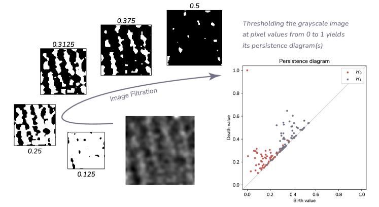
Figure 1: An illustration of the 0- and 1-dimensional persistence diagrams of the sublevel set filtration of a grayscale image. Pixel values at which images were binarized can be seen next to the binarized images.

3.2 Images

To move forward we must define what we mean by an image. An $(k\times l)$ image in this setup is most simply taken to be a vector $\tilde{\bm{x}}_{i}\in\mathbb{R}^{kl}$, where $k$ is the number of rows (# of vertical pixels) in the image and $l$ is the number of columns (# of horizontal pixels). If $\bar{\mathbb{R}}=[-\infty,\infty]$ then by considering blocks in the vector $\tilde{\bm{x}}_{i}$ of length $l$, we may naturally embed $\tilde{\bm{x}}_{i}$ into $\{f\mathrel{\mathop{\mathchar 58\relax}}\mathbb{Z}^{2}\to\bar{\mathbb{R}}\}$—identifying some pixel with the origin. Now in $\mathbb{Z}^{2}$, where spatial information makes sense, it is useful to have another definition at hand for the computation of PH. We follow the lead of Thomas et al. (2023), in defining a (2-dimensional) image map to be a function $I\mathrel{\mathop{\mathchar 58\relax}}\mathbb{Z}^{2}\to\bar{\mathbb{R}}$, where $I(p)=-\infty$ indicates that $p$ is a black pixel and $I(p)=\infty$ indicates that $p$ is a white pixel. The smallest rectangle with integer coordinates $[k,k+m]\times[l,l+n]\subset\mathbb{R}^{2}$ which contains all the black pixels—i.e. on which $I<\infty$—will be denoted the image set or simply the image. As previously mentioned, for the purposes of cubical homology and persistence we must derive cubical sets from the image map $I$. We accomplish this by the construction of another function $I^{\prime}$ on the family of unit squares with integer vertices. For any such $\tau=[i,i+1]\times[j,j+1]$ we define our filtration function to be

$$I^{\prime}(\tau)\mathrel{\mathop{\mathchar 58\relax}}=I(i,j).$$

For lower dimensional elementary cubes $\tau$, such as intervals or vertices, we define the value of $I^{\prime}$ to be the minimum $I(i,j)$ such that $\tau\subset[i,i+1]\times[j,j+1]$. This is consistent with the definition used in the persistent homology software GUDHI Python library, which we use for our PH calculation (Dłotko, 2015). We consider the homology of sublevel set filtrations. That is, we look at the homology of each cubical set

$$\{\tau\equiv[i,i+1]\times[j,j+1]\mathrel{\mathop{\mathchar 58\relax}}I^{\prime}(\tau)\leq t\},$$

which may naturally be considered as a binary image (each pixel corresponding to a $\tau$). Treating pixels as unit squares (i.e. top-dimensional) rather than elements of $\mathbb{Z}^{2}$ (i.e. vertices) is also known as the $T$-construction (Garin et al., 2020).

3.3 Persistent homology

Consider the collection of binary images (i.e. cubical complexes) $\mathcal{I}=\{I_{t}\}_{t\in\mathbb{R}}$, where

$$I_{t}\mathrel{\mathop{\mathchar 58\relax}}=\bigcup_{(i,j)\in I^{-1}([0,t])}[i,i+1]\times[j,j+1],$$

or equivalently, $I_{t}=I^{\prime-1}([0,t]).$ When $s\leq t$ we have $I_{s}\subset I_{t}$ and hence $\mathcal{I}=\{I_{t}\}_{t\in\mathbb{R}}$ defines a filtration of cubical complexes. Given the inclusion maps $\iota_{s,t}\mathrel{\mathop{\mathchar 58\relax}}I_{s}\to I_{t}$, for $s\leq t$ there exist linear maps between all homology groups

$$f^{s,t}_{k}\mathrel{\mathop{\mathchar 58\relax}}H_{k}(I_{s})\to H_{k}(I_{t}),$$

which are induced by $\iota_{s,t}$ (see chapter 4 of Kaczynski et al., 2004). The persistent homology groups of the filtered image $\mathcal{I}$ are the quotient vector spaces $\mathrm{im}\,f^{s,t}_{k}$ whose elements represent shape features—such as connected components or holes—called cycles that are “born” in or before $I_{s}$ and that “die” after $I_{t}$. The dimensions of these vector spaces are the persistent Betti numbers $\beta_{k}^{s,t}$. Heuristically, a cycle (more correctly an equivalence class of cycles) $\gamma\in H_{k}(I_{s})$ is born at $I_{s}$ if it appears for the first time in $H_{k}(I_{s})$—formally, $\gamma\not\in H_{k}(I_{r})$, for $r<s$. The cycle $\gamma\in H_{k}(I_{s})$ dies entering $I_{t}$ if it merges with an older cycle (born at or before $s$) entering $H_{k}(I_{t})$. The $k^{th}$ persistent homology of $\mathcal{I}$, denoted $PH_{k}$, is the collection of homology groups $H_{k}(I_{t})$ and maps $f_{s,t}^{k}$, for $-\infty\leq s\leq t\leq\infty$. All of the information in the persistent homology groups is contained in a multiset in $\mathbb{R}^{2}$ called the persistence diagram (Edelsbrunner and Harer, 2010).

We will denote the $k^{th}$ persistence diagram of $\mathcal{I}$ as $\mathcal{D}^{k}$. The persistence diagram $\mathcal{D}^{k}$ consists of the points $(b,d)$ with multiplicity equal to the number of the cycles that are born at $I_{b}$ and die entering $I_{d}$. Figure 1 contains an illustration of the persistence diagrams associated to a filtration of a given greyscale image. We will only consider $\mathcal{D}^{0}$ and $\mathcal{D}^{1}$ in this study because higher-dimensional persistence diagrams are trivial for cubical filtrations of 2-dimensional images. For this particular setup, if $(b,d)\in\mathcal{D}^{0}$, this indicates there is a local minimum of the image $\mathcal{I}$ at some pixel $p^{+}$ with $I^{\prime}(p^{+})=b$ and $d$ represents the greyscale threshold at which the connected component containing $p$ merges with a connected component containing a local minimum with birth time less than $b$. In this case, $p^{+}$ is called a positive cell and gives birth to a connected component in $PH_{0}$. Furthermore, we can also find an interval $\tau^{-}$ (negative cell) that kills such a feature, i.e. $I^{\prime}(\tau^{-})=d$ (cf. Boissonnat et al., 2018). An analogous result holds that local maxima kill loops/holes in $PH_{1}$.

3.4 Preliminary image processing

Before calculating topological statistics of images in Section 3.5, we must make sure that the image is processed so that the output topological signal is as strong as possible. We consider the simple setup of $n$ image observations $\tilde{\bm{x}}_{1},\dots,\tilde{\bm{x}}_{n}$. As in Thomas et al. (2023), the images we consider here have been smoothed by a separable Gaussian filter with $\sigma=2$ (which yielded strong results in the same article); however, the $\sigma$ you choose ought to depend on the degree of noise in the image and may be calibrated by the elbow method for a pre-chosen linear combination of topological statistics (ibid.). As we can consider the images as functions from $\mathbb{Z}^{2}$ to $\bar{\mathbb{R}}$, we may calculate 0 and 1-dimensional sublevel set persistence diagrams according to cubical homology—which we will denote $\mathcal{D}^{0}_{i}$ and $\mathcal{D}^{1}_{i}$ respectively. Denote $\mathrm{PD}$ to be the space of persistence diagrams. We then calculate some summary $f\mathrel{\mathop{\mathchar 58\relax}}\mathrm{PD}^{2}\to\mathbb{R}^{d}$ from this 2-tuple of persistence diagrams to a $d$-tuple of real numbers, $d\geq 1$. Linear functionals of the features

$$\bm{x}_{i}\equiv\psi(\tilde{\bm{x}}_{i})\mathrel{\mathop{\mathchar 58\relax}}=f\big{(}\mathcal{D}^{0}_{i},\mathcal{D}^{1}_{i}\big{)},\quad i=1,\dots,n,$$

are supposed to better represent the change than any linear functionals of the image itself. Though detecting topological change is our main focus, $\psi\mathrel{\mathop{\mathchar 58\relax}}\mathbb{R}^{kl}\to\mathbb{R}^{d}$ can be arbitrary in the exposition below. In particular we assume that if a changepoint $\kappa<n$ is present then it is represented in the univarate change in distribution of some linear functional of $\psi(\tilde{\bm{x}}_{i})$. As the main objective is to recover changes dictated by shape features, throughout this article will we take the mean pixel intensity across the image $\tilde{\bm{x}}_{i}$ to equal 0, i.e.

$$\frac{1}{kl}\sum_{j=1}^{kl}\tilde{\bm{x}}_{ij}\equiv 0,$$

and the variance of the pixel intensities to equal 1, i.e.

$$\frac{1}{kl}\sum_{j=1}^{kl}\tilde{\bm{x}}_{ij}^{2}\equiv 1.$$

In practice, topological features may correlate with the mean and intensity of images. For example, in the solar flare example of Zheng et al. (2023) (taken from Xie et al., 2012), the mean and the variance of the pixel intensities are highly correlated with the occurrence of a solar flare event. For instance, certain regions within the image increase in luminance, and often the number of bright areas increase in number as well. Removing the effect of mean and variance from our image series is a way to ensure that we capture purely topological change. Doubtless histogram equalization or other partial contrast matching methods may be used for other tasks (Szeliski, 2022).

3.5 Crafting a topological feature mapping

For any fixed $d\geq 1$, there are uncountably many distinct functions $f\mathrel{\mathop{\mathchar 58\relax}}\mathrm{PD}^{2}\to\mathbb{R}^{d}$ we could choose. Thus, finding a good function $f$ is a nontrivial task. The article by Obayashi et al. (2018) served as one of the points of departure for this article. The authors use persistence images (Adams et al., 2017) as their functional which—in concert with logistic regression—yield “hotspots” on a dual persistence image reconstructed from $\bm{\beta}$. However, they consider only labelled data for their learning task, and provide no estimates of uncertainty for their recovered coefficients $\bm{\beta}$. We do not use persistence images here, but we do describe a feature embedding $f_{\text{PI}}$ and demonstrate that persistence images are capable of recovering the locations of a topological change in Section S4 of the Supplementary Material.

The approach that we consider is to select a topological feature embedding which represents a wide range of topological summary statistics from Chung et al. (2018), wherein the statistics we describe were shown to achieve strong test accuracy in a support vector machine classification task of skin lesions. We will use the same suite of persistence statistics used by Chung et al. (2018), along with the ALPS statistic introduced in Thomas et al. (2023). Namely, we define $l_{i}=d_{i}-b_{i}$ and $m_{i}=(d_{i}+b_{i})/2$ and construct our topological embedding $f_{\text{stat}}$ to have the form

$$f_{\text{stat}}\big{(}\mathcal{D}^{0},\mathcal{D}^{1}\big{)}\mathrel{\mathop{\mathchar 58\relax}}=(T_{j})_{1\leq j\leq 36},$$

with $T_{j}$ equal to the following statistics of the empirical distributions of $l_{i}$ and $m_{i}$ for the persistence diagrams $\mathcal{D}^{0}$ and $\mathcal{D}^{1}$. The various $T_{j}$ are the mean of $l_{i}$ and $m_{i}$ for $\mathcal{D}^{0}$ and $\mathcal{D}^{1}$; variance of $l_{i}$ and $m_{i}$ for $\mathcal{D}^{0}$ and $\mathcal{D}^{1}$; skewness of $l_{i}$ and $m_{i}$ for $\mathcal{D}^{0}$ and $\mathcal{D}^{1}$; kurtosis of $l_{i}$ and $m_{i}$ for $\mathcal{D}^{0}$ and $\mathcal{D}^{1}$; $\bm{25^{th}}$, $\bm{50^{th}}$, and $\bm{75^{th}}$ percentiles of $l_{i}$ and $m_{i}$ for $\mathcal{D}^{0}$ and $\mathcal{D}^{1}$; interquartile range of $l_{i}$ and $m_{i}$ for $\mathcal{D}^{0}$ and $\mathcal{D}^{1}$; persistent entropy of $l_{i}$ for $\mathcal{D}^{0}$ and $\mathcal{D}^{1}$; and ALPS statistic of $l_{i}$ for $\mathcal{D}^{0}$ and $\mathcal{D}^{1}$.

For a large class of persistence statistics, we can establish their stability using Theorem 3 of Divol and Polonik (2019) in conjunction with Theorem 5.1 of Skraba and Turner (2022). This means that even in the presence of a moderate amount of noise, if a “separability” condition holds with high probability (as in Proposition 2.2), our algorithm will return the correct changepoint as the posterior mode of $\pi(\kappa\mid\bm{\beta},\bm{X})$.

4 Simulation & Applications

To demonstrate the utility of our method, we consider a simple simulated setup and evaluate our method against other well-known methods in the multivariate changepoint literature. We consider both a straightforward and a more difficult (noisier) changepoint problem for a topological change in a rather short image series. This is to show that our topological feature embedding needs relatively little data to perform well, and that our changepoint method also performs well and is robust in this “small” data setting.

4.1 Simulation

For our simulation, we consider a sequence of 50 random images $\tilde{X}_{i}$, $i=1,\dots,50$ of size $50\times 50$ each consisting of i.i.d. standard Gaussian noise. For ease of notation, we will denote the random image $\tilde{X}_{i}$ as $X_{i}$. For ease of exposition we begin by examining our method on a single image series $V^{(1)}=\big{(}X^{(1)}_{i}\big{)}_{1\leq i\leq 50}$. Initially, we consider a changepoint $\kappa^{*}=25$, whereafter a random rectangular region with intensity of $-2$ is added to each $X^{(1)}_{i}$. Namely, if $X^{(1)}_{ijk}$ is the pixel at row $j$ and column $k$ of the image $X^{(1)}_{i}$, we have that

$$X^{(1)}_{ijk}=\begin{cases}Z_{ijk}-2&\mbox{ if }L_{1}-W_{1}\leq j\leq L_{1}+W_{1},L_{2}-W_{2}\leq k\leq L_{2}+W_{2}\\ Z_{ijk}&\mbox{ otherwise }\end{cases},$$

where $Z_{ijk}$ are i.i.d. $N(0,1)$ for $1\leq i,j,k\leq 50$, $L_{m}$, $W_{m}$ are independent and uniformly distributed on $\{5,6,\dots,43,44\}$ and $\{2,3,4\}$ respectively, for $m=1,2$. Note that $V^{(1)}=(X^{(1)}_{ijk})_{1\leq i,j,k\leq 50}$. The additional 1000 videos we simulate according to this formula will be called Experiment 1.

Examining these images without noise yields a sequence before the changepoint corresponding to no sublevel set homology, and a distribution after the changepoint corresponding to a randomly located connected component with lifetime equal to 2. As in Section 3.4, we standardize each of the images $X_{i}$ to have mean pixel intensity 0 and standard deviation 1. As such, any estimated change in mean or variance of the image series is entirely spurious and we will be less likely to capture change that is not purely topological. Images of the video before and after the changepoint for this initial scenario can be seen in Figure 2.

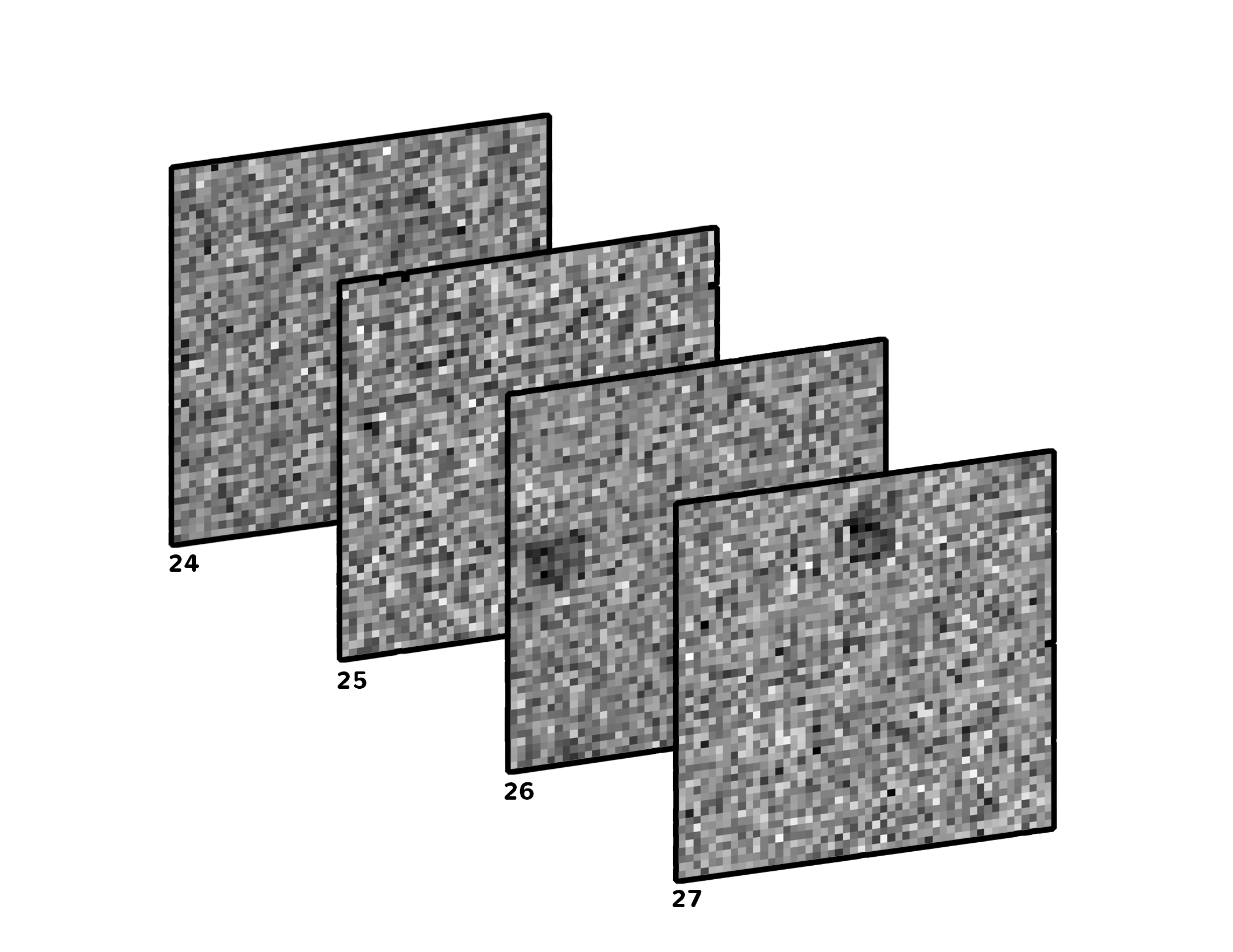
Figure 2: Frames 24–27 of the first simulated video $V^{(1)}$ where $\kappa^{*}=25$ and $n=50$. The changepoint manifests as a darkening of a small region in frames 26 and 27 (and beyond).

We compare our method—which we deem bclr—to the random forest based classification changepoint detection method from the changeforest package (Londschien et al., 2023) (which we deem cf in the sequel); the E-divisive method from the ecp package (James and Matteson, 2015; Matteson and James, 2014); and, the kcp kernel change-point method from Arlot et al. (2019) as implemented in the ruptures package (Truong et al., 2020). To demonstrate the dual benefit of our approach in conjunction with TDA, we gave our method the TDA features from $f_{\text{stat}}$, and the other methods dimensionality-reduced features by first vectorizing our images and then projecting them down onto their first 36 principal components. We did consider a Bayesian changepoint method with available code, but this did not perform well. Information about this and the parameters used for each model can be seen in Section S2 of the Supplementary Material.

We also devised new topologically-aware versions of cf, ecp, and kcp—where we fed these algorithms the same topological features from $f_{\text{stat}}$. We christened these methods cf+TDA, ecp+TDA, and kcp+TDA respectively. Each algorithm received the exact same PCA and normalized TDA features. We took the estimated changepoint $\hat{\kappa}$ to be the posterior mode in our setup. For our method, we always took the 2500 posterior samples for both $\kappa$ and $\bm{\beta}$ after the burn-in period (more details on the properties of the Gibbs sampler and its convergence are available in Section S2 of the Supplementary Material).

For the image series $V^{(1)}$ the estimated posterior change distribution using our algorithm can be seen in Figure 3 (left). On the other hand, running cf and ecp algorithms on the PCA features yields an estimate of no changepoint ($p$-value = 0.3 for cf and 0.795 for ecp). There is no $p$-value provided for kcp, but the estimated changepoint was frame 15. However, as one can see from Figure 3 (right), we are not too far from the ground truth if we instead use the PCA features in conjunction with our method. The topologically-aware methods cf+TDA, kcp+TDA, and ecp+TDA perform quite well for the image series $V^{(1)}$, recovering the changepoint $\kappa^{*}$ present at $\kappa=25$.

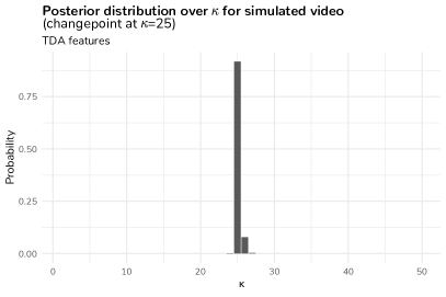
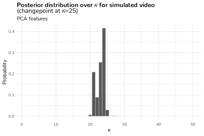
Figure 3: The posterior distribution $\pi(\kappa\mid x)$ for the first simulated video $X^{(1)}$ with $\kappa^{*}=25$. Note that even with the PCA features, our method gets close to the true changepoint at $\kappa^{*}=25$.

We also investigate a second image series $V^{(2)}=(X^{(2)}_{ijk})_{1\leq i,j,k\leq 50}$ with a changepoint at $\kappa^{*}=40$ and $X^{(2)}_{ijk}=Z_{ijk}+1$ instead of $Z_{ijk}-2$. The additional 1000 videos we simulate according to this formula will be called Experiment 2. For this single random image series we see similar results. All of our topological methods detect the changepoint, but at much lower levels of significance across the board ($p$-value = 0.035 for cf+TDA and 0.05 for ecp+TDA). The methods without the TDA features return changepoints at 1 for cf ($p$-value = 0.3), 46 for ecp ($p$-value 0.805) and 15 for kcp.

To verify that our bclr method performs well for more than just two videos, we generated 1000 additional random image series $V^{(1)}$ (Experiment 1) and $V^{(2)}$ (Experiment 2) and gauged the behavior of the various methods in both scenarios. For each of the methods, we then calculated the accuracy of the estimated changepoint $\hat{\kappa}$ in terms of proportion of times the estimated changepoint was exactly correct (“% Exact”) and the root mean-squared error, or “RMSE” (of the estimated changepoint from $\kappa^{*}=25,40$). For our bclr method we calculated the RMSE within each of the posterior samples of length 2500 and report the mean RMSE across all 1000 simulations as well as its standard error.

We gave the same 36-dimensional normalized TDA features to each of the TDA methods, as well as the same first 36 principal components of the image to the other methods. The results of Experiment 1 can be seen in Table 1.

Method	bclr	cf+TDA	ecp+TDA	kcp+TDA	cf	ecp	kcp
% Exact	0.697	0.714	0.663	0.673	0.020	0.036	0.009
	(0.015)	(0.014)	(0.015)	(0.015)	(0.004)	(0.006)	(0.003)
RMSE	0.948	1.021	1.614	1.382	16.998	13.222	15.365
	(0.783)	—	—	—	—	—	—

Table 1: % Exact and RMSE for 1000 simulated videos across five changepoint methods in the case of $\kappa^{*}=25$ and $X_{ijk}=Z_{ijk}-2$ for seven different changepoint methods. Standard errors for % Exact and RMSE indicated in parentheses. SEs for RMSE not applicable for the other methods.

First, the methods that we have developed to include the TDA features vastly outperform the ones that only use the PCA features. There hardly seems to be any signal at all for the methods applied to the conventional PCA features, and in fact the results are hardly any different from a uniform random choice. Though all of the methods with the TDA features perform well, our method evinces the smallest RMSE. This demonstrates not only the utility of the topological features but the additional ability of our changepoint method to yield consistent results.

If we denote $p_{\ell}$ to be the probability mass function of $\pi(\kappa\mid\bm{X}_{\ell})$ as estimated from the MCMC output, where $\bm{X}_{\ell}$ are the features for simulated video $\ell=1,\dots,1000$, then we may use $p_{\ell}$ to derive quantiles

$$q_{\alpha}^{(\ell)}\mathrel{\mathop{\mathchar 58\relax}}=\inf\{\kappa\mathrel{\mathop{\mathchar 58\relax}}\sum_{i=1}^{\kappa}p_{\ell}(i)\geq\alpha\},$$

and thus form a posterior credible interval

$$I_{\alpha,\ell}\mathrel{\mathop{\mathchar 58\relax}}=\big{[}q_{\alpha/2}^{(\ell)},q_{1-\alpha/2}^{(\ell)}\big{]}$$

for the true changepoint $\kappa^{*}=25$ for each simulated video. We examine the coverage probability, i.e.

$$\mathbb{P}(\kappa^{*}\in I_{\alpha})\approx\frac{1}{1000}\sum_{\ell=1}^{1000}\mathbf{1}\big{\{}\kappa^{*}\in I_{\alpha,\ell}\big{\}}$$

for bclr applied to both the TDA and PCA features in Table 2.

	$\mathbb{P}(\kappa^{*}\in I_{\alpha})$
$(1-\alpha)\times 100\%$	50%	80%	90%	95%	99%
TDA	0.852	0.933	0.964	0.972	0.994
PCA	0.312	0.509	0.594	0.645	0.721

Table 2: Estimated credible interval coverage probabilities for $\kappa^{*}=25$ for our bclr method.

Even though $\kappa$ is discrete, the credible intervals for the TDA features in our setup are conservative at each setting of $\alpha$ that we consider. Though the specified intervals do not even necessarily have the highest posterior mass (we do this in Table S3 and see similar results), Table 2 indicates that interval estimation using bclr with TDA features is appropriate here (where the signal is fairly strong relative to the noise), in a way that imposes no distributional restrictions on the data $\bm{X}$. A detailed analysis of these intervals can be seen in Section S3 of the Supplementary Material. For Experiment 2 ($\kappa^{*}=40$) the signal is cut in half, and corresponding the coverage probabilities are less than their nominal amount—see Table S4. Nevertheless, the probability our method will return an estimate containing the true changepoint is higher than the other methods do to our ability to seemlessly carry out interval estimation.

As a proof-of-concept, we may use the posterior sample estimates of the mean and covariance we gained from the single image series $V^{(2)}$ as a prior for $\bm{\beta}$ for the 1000 videos in Experiment 2. We considered this additional prior for $\bm{\beta}$ for our method to see if this additional information provides us further ability to discriminate the changepoint location accurately. What we call the “data-driven prior” was a multivariate normal with mean equal to the posterior sample mean and covariance equal to the sample covariance of $\bm{\beta}$ from the initial simulated video with $\kappa^{*}=40$. We denote the method corresponding to this prior as bclr-2. The other prior we deemed the “simple prior”, where the prior was our default of $\bm{\beta}\sim N(0,3I_{d})$. The method corresponding to this prior is called bclr-1.

In the scenario with the data-driven prior, we also conducted 5000 Monte Carlo iterations and chose the 2500 simulations after the burn-in. As one can see in Table 3, where all the results are listed, our method using the posterior mode as changepoint estimate performs comparably to the kcp+TDA and ecp+TDA methods and vastly outperforms the non-topological versions of those methods as well as all versions of cf.

Method	bclr-1	bclr-2	cf+TDA	ecp+TDA	kcp+TDA	cf	ecp	kcp
% Exact	0.334	0.508	0.458	0.520	0.534	0.020	0.020	0.019
	(0.015)	(0.016)	(0.016)	(0.016)	(0.016)	(0.004)	(0.004)	(0.004)
RMSE	4.498	2.547	5.030	4.330	3.300	21.191	19.009	21.729
	(4.649)	(2.362)	—	—	—	—	—	—

Table 3: % Exact and RMSE for 1000 simulated videos across seven changepoint methods in the case of $\kappa^{*}=40$ and $X_{ijk}=Z_{ijk}+1$. The methods bclr-1 and bclr-2 correspond to the bclr methods with the simple and data-driven priors respectively. Standard errors for % Exact and RMSE indicated in parentheses. SEs for RMSE not applicable for the other methods.

Furthermore, none of other methods we describe tell us what coordinates are most important for detecting such a change. With regards to the 1000 simulated videos in Experiment 1 (and $\kappa^{*}=25$) we measured the importance of a given coordinate of $\bm{\beta}$ with respect to the TDA features via the mean and signal-to-noise ratio (SNR). We can see the mean and standard deviation of the SNRs—for persistence statistics which had the highest SNR most often among the 1000 simulations—in Table 4. Beyond this, we also were able to get the mean posterior correlations for the regression coefficients corresponding to the persistence statistics. The largest absolute mean correlation among the 5 statistics in Table 4 was -0.358 between kurtosis and skewness of the lifetimes for $\mathcal{D}_{0}$. The smallest absolute mean correlation was -0.007 between the ALPS statistic and the persistent entropy. The other absolute mean correlations hovered between 0.043 and 0.2, which indicates that there was not necessary a single statistic which stood out above the rest and justified the inclusion of multiple statistics and thus our feature embedding $f_{\text{stat}}$.

The ability of our method to determine which coordinate is important has further utility than the detection of a topological change. Section S1.1 of the Supplementary Material shows the efficacy of our method in detecting where and how a change in data of mixed type occurs. In the following subsection (Section S1.2) we demonstrate that our method can not only detect a change in covariance via a degree-2 polynomial feature embedding, but do better than any other advanced nonparametric method.

Statistic	Prop. highest SNR	Mean (SD) Posterior SNR
persistent entropy of $l_{i}$ for $\mathcal{D}^{0}$	0.185	1.562 (1.082)
skewness of $l_{i}$ for $\mathcal{D}^{0}$	0.156	1.873 (0.817)
kurtosis of $l_{i}$ for $\mathcal{D}^{0}$	0.120	1.734 (0.875)
ALPS statistic of $l_{i}$ for $\mathcal{D}^{0}$	0.114	1.118 (1.218)
variance of $l_{i}$ for $\mathcal{D}^{0}$	0.111	1.703 (0.683)

Table 4: Table of posterior coefficient signal-to-noise ratios for 1000 simulated videos with $\kappa^{*}=25$ along with proportion (out of 1000 simulations) in which said statistic had the highest SNR.

4.2 Applications

Evidence presented in Thomas et al. (2023) indicates that a reasonable topological summary for the detection of nanoparticle dynamics is some linear combination of the ALPS statistic (ibid.) and persistent entropy (Atienza et al., 2020). We assess the accuracy of this statement using the topological embedding $f_{\text{stat}}$. Visual inspection of the nanoparticle video of interest suggests that a change occurs in the vicinity of frame 210, though the high signal-to-noise ratio precludes any notion of “ground truth”. Thus, we apply our algorithm to the data to get an estimate of where the change occurs and what the best representation for said change is. Plots describing these results can be seen in Figure 4 and averages of 5 consecutive frames (to improve visualization) before and after the estimated changepoint can be seen in Figure 5. We choose a prior for $\beta$ with mean 0 and covariance matrix equal to $3I_{d}$, where $I_{d}$ is the $d$-dimensional identity matrix.

As seen in Figure 4, the marginal posterior distribution of $\kappa$ concentrates around frame 210. After having run our Gibbs sampler for 5000 iterations and discarding the first 2500 samples from the posterior, we estimate that $\pi(210\mid\bm{X})=0.3560$, $\pi(211\mid\bm{X})=0.3112$, and $\pi(214\mid\bm{X})=0.2984$ with probability less than $0.02$ elsewhere. We can see using the posterior mean of $\bm{\beta}$ that reasonable separation is achieved for $\bm{x}_{\kappa}^{\top}\bm{\beta}$ in Figure 4 (bottom). The question still remains as to which topological statistics best represent the change. We summarize the importance of a given coordinate of $\bm{\beta}$ by its signal-to-noise ratio (SNR), defined in the previous section. The top 5 statistics in terms of signal-to-noise ratio can be seen in Table 5.

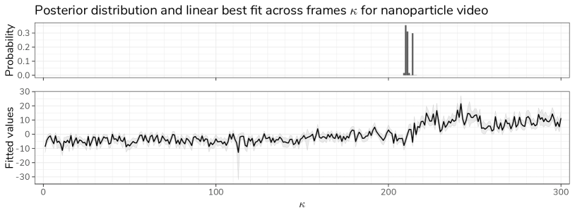
Figure 4: Nanoparticle data. (Top) the posterior distribution (over last 2500 Gibbs sampler draws) of $\kappa$. (Bottom) the fitted values $\bm{x}_{\kappa}^{\top}\bm{\beta}$ for the last 2500 draws of $\bm{\beta}$. 95% credible bands depicted in light gray.

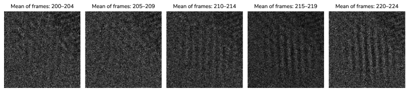
Figure 5: Frame-averaged nanoparticle video. One can see the lack of crystalline structure prior to frame 210 and the presence of structure afterwards.

Statistic	Posterior SNR	Posterior mean
$\bm{25^{th}}$ percentile of $l_{i}$ for $\mathcal{D}^{1}$	5.694	1.087
variance of $l_{i}$ for $\mathcal{D}^{0}$	3.772	2.389
persistent entropy of $l_{i}$ for $\mathcal{D}^{1}$	3.407	-1.481
persistent entropy of $l_{i}$ for $\mathcal{D}^{0}$	2.117	-0.905
ALPS statistic of $l_{i}$ for $\mathcal{D}^{0}$	1.890	-1.222

Table 5: Table of posterior coefficient statistics for nanoparticle video.

The results of Table 5 support—but also refine—the results of Thomas et al. (2023), wherein the persistent entropy and the ALPS statistic of the lifetimes of $\mathcal{D}^{0}$ were chosen to represent the dynamics of the nanoparticle. These results seem to suggest that the variance of $l_{i}$ of $\mathcal{D}^{0}$ captures the dynamics even better, having a large posterior mean and rather low variance. For the sake of comparison, we ran ecp+TDA, cf+TDA, and kcp+TDA and recovered an estimated changepoint of $\hat{\kappa}=214$ in the first two cases with $p$-values of 0.005 (for both methods) and $\hat{\kappa}=215$ for kcp.

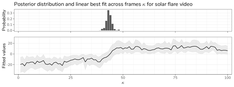
Figure 6: Solar flare data. (Top) the posterior distribution (over last 2500 Gibbs sampler draws) of $\kappa$. (Bottom) the fitted values $\bm{x}_{\kappa}^{\top}\bm{\beta}$ for the last 2500 draws of $\bm{\beta}$. 95% credible bands depicted in light gray.

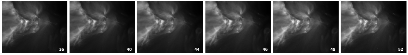
Figure 7: Standardized/normalized solar flare images. Flare event seems to occur in early portion of 40s frames. The change in intensity seems to be pre-empted by a topological change, as detected by bclr.

We conclude this section by looking at a 100 frame solar flare video, which was taken from Xie et al. (2012) and analyzed via the online changepoint method PERCEPT proposed in Zheng et al. (2023). Running our changepoint method with the same prior as in the case of the nanoparticle video, we observe a posterior mode of $\hat{\kappa}=44$ using our topological representation (see histogram (top) in Figure 6). However, using the pixel means of the images as a one-dimensional signal to detect the solar flare the estimated posterior mode of $\pi(\kappa\mid\bm{X})$ is $\kappa=46$. This seems reasonable given the below results for the other methods. In the article (Zheng et al., 2023), the changepoint was estimated to be $\kappa=49$ using their topological online changepoint detection method PERCEPT. Since they were using a CUSUM approach on their derived topological features, their estimate was more likely to occur after the best separation between pre- and post-change distributions. Also, there is no indication in the article that their images were standardized, which leads one to believe that their estimated changepoint captures mostly the increase in the mean intensity of the solar flare video. That being said, using the PCA features described below, our method has posterior mode $\hat{\kappa}=49$. The discrepancy between the estimate of the changepoint using topological statistics and pixel means suggests that there is topological change occurring prior to the eruption which ultimately takes place and leads to a great increase in radiation which is visually apparent.

We also extract 30 principal components from the solar flare image data, as in Zheng et al. (2023). This yields an estimated 17 changepoints at significance level $\alpha=0.02$ using cf. However, the first changepoint is estimated to be 47. The PCA features yield estimated changepoints at $\kappa=33$ and 63 for ecp (with $p$-values 0.005 for each). The method kcp yields an initial changepoint of 45 using the PCA features. Using these PCA features with bclr tells us there is a posterior probability of at least 95% that the changepoint lies in the interval $[46,54]$ (using the posterior quantile intervals above). This robustness—in terms of increased uncertainty—to misspecification of feature embedding can be very useful when we are not dealing with image data, are worried about false positives, or surmise there is no topological change.

5 Conclusion

In this article, we have presented a Bayesian changepoint method that utilizes logistic regression to detect changes in an interpretable and parsimonious fashion while imposing few assumptions on the data-generating process. Our method also learns the nature of the changepoint and provides uncertainty quantification on both the location of change and the coordinates in which the change occurs. We have also provided a canonical topological feature embedding for detecting changes in image series that outperforms standard Euclidean features and have demonstrated our method’s competitive performance on a variety of tasks.

The Bayesian changepoint method introduced in this article could be extended in a number of different directions:

Alternative classifiers. We could consider alternatives to the combination of a logistic regression model with a multivariate normal prior. For example, we expect that choosing a prior distribution that induces sparsity in the regression coefficients (Carvalho et al., 2010; Mitchell and Beauchamp, 1988; Xu and Duan, 2023) would lead to improved inferences and greater interpretability for high-dimensional time series. To capture complex changes with less feature engineering (at the expense of some interpretability), we could replace the logistic regression model with a more flexible classifier based on Bayesian additive regression trees (Chipman et al., 2010) or kernel methods (Zhu and Hastie, 2005; Shawe-Taylor and Cristianini, 2004).

More complex data types. As we have emphasized through the article, the proposed Bayesian changepoint method treats the observed time series as a sequence of covariate vectors. As a result, there is no need to specify a model for the data, and the method can be applied to data of mixed type. For these same reasons, we expect the method could be extended in a conceptually straightforward way to handle more complex data types such as time-indexed network, functional, or shape data.

Multiple changepoints. Extending the proposed method to the multiple changepoint setting is a high priority. A natural approach would be to allow the latent variables $Y_{1},\ldots,Y_{n}$ to take values in the set $\{0,1,2,\ldots,L\}$ where $L$ is the number of changepoints. In that case, the logistic regression model could be replaced with a multinomial logistic regression model. In many applied settings, including some of the examples discussed in this article, a time series alternates between two possible states: a normal, baseline state and an abnormal, outlier state. See, for example, Bardwell and Fearnhead (2017). We could address this problem using the proposed Bayesian changepoint framework by conditioning on a larger set $\Gamma_{n,L}$ that includes sequences of zeros and ones with at most $L$ changes.

We intend to pursue these extensions in future work.

References

- Adams et al. (2017) Henry Adams, Tegan Emerson, Michael Kirby, Rachel Neville, Chris Peterson, Patrick Shipman, Sofya Chepushtanova, Eric Hanson, Francis Motta, and Lori Ziegelmeier. Persistence images: A stable vector representation of persistent homology. Journal of Machine Learning Research, 18, 2017.
- Allen et al. (2018) David E Allen, Michael McAleer, Robert J Powell, and Abhay K Singh. Non-parametric multiple change point analysis of the global financial crisis. Annals of Financial Economics, 13(02):1850008, 2018.
- Arlot et al. (2019) Sylvain Arlot, Alain Celisse, and Zaid Harchaoui. A kernel multiple change-point algorithm via model selection. Journal of machine learning research, 20(162), 2019.
- Atienza et al. (2020) Nieves Atienza, Rocío González-Díaz, and Manuel Soriano-Trigueros. On the stability of persistent entropy and new summary functions for topological data analysis. Pattern Recognition, 107:107509, 2020.
- Balaji et al. (2018) M. Balaji, Arun Chakraborty, and M. Mandal. Changes in tropical cyclone activity in north indian ocean during satellite era (1981–2014). International Journal of Climatology, 38(6):2819–2837, 2018. doi: https://doi.org/10.1002/joc.5463.
- Bardwell and Fearnhead (2017) Lawrence Bardwell and Paul Fearnhead. Bayesian Detection of Abnormal Segments in Multiple Time Series. Bayesian Analysis, 12(1):193 – 218, 2017. doi: 10.1214/16-BA998.
- Barry and Hartigan (1993) Daniel Barry and J.A. Hartigan. A bayesian analysis for change point problems. Journal of the American Statistical Association, 88(421):309–319, 1993.
- Bhattacharyya and Johnson (1968) G. K. Bhattacharyya and Richard A. Johnson. Nonparametric tests for shift at an unknown time point. The Annals of Mathematical Statistics, 39(5):1731–1743, 1968. ISSN 00034851.
- Boissonnat et al. (2018) Jean-Daniel Boissonnat, Frédéric Chazal, and Mariette Yvinec. Geometric and topological inference, volume 57. Cambridge University Press, 2018.
- Brodsky and Darkhovsky (1993) Emily Brodsky and Boris S. Darkhovsky. Nonparametric methods in change point problems, volume 243. Springer Science & Business Media, 1993.
- Carlin et al. (1992) Bradley P. Carlin, Alan E. Gelfand, and Adrian F.M. Smith. Hierarchical Bayesian Analysis of Changepoint Problems. Journal of the Royal Statistical Society: Series C (Applied Statistics), 41(2):389–405, 1992. doi: https://doi.org/10.2307/2347570.
- Carvalho et al. (2010) Carlos M. Carvalho, Nicholas G. Polson, and James G. Scott. The horseshoe estimator for sparse signals. Biometrika, 97(2):465–480, 2010. ISSN 00063444, 14643510.
- Chazal and Michel (2021) Frédéric Chazal and Bertrand Michel. An introduction to topological data analysis: fundamental and practical aspects for data scientists. Frontiers in artificial intelligence, 4:667963, 2021.
- Chen and Gupta (2012) Jie Chen and Arjun K. Gupta. Parametric statistical change point analysis: with applications to genetics, medicine, and finance. 2012.
- Chipman et al. (2010) Hugh A. Chipman, Edward I. George, and Robert E. McCulloch. BART: Bayesian additive regression trees. The Annals of Applied Statistics, 4(1):266 – 298, 2010. doi: 10.1214/09-AOAS285.
- Chung et al. (2018) Yu-Min Chung, Chuan-Shen Hu, Austin Lawson, and Clifford Smyth. Topological approaches to skin disease image analysis. In 2018 IEEE International Conference on Big Data (Big Data), pages 100–105. IEEE, 2018.
- Corradin et al. (2022) Riccardo Corradin, Luca Danese, and Andrea Ongaro. Bayesian nonparametric change point detection for multivariate time series with missing observations. International Journal of Approximate Reasoning, 143:26–43, 2022.
- Divol and Polonik (2019) Vincent Divol and Wolfgang Polonik. On the choice of weight functions for linear representations of persistence diagrams. Journal of Applied and Computational Topology, 3(3):249–283, September 2019. ISSN 2367-1734. doi: 10.1007/s41468-019-00032-z.
- Dłotko (2015) Pawel Dłotko. Cubical complex. In GUDHI User and Reference Manual. GUDHI Editorial Board, 2015.
- Edelsbrunner and Harer (2010) Herbert Edelsbrunner and John Harer. Computational topology: an introduction. American Mathematical Society, Providence, Rhode Island, 2010.
- Fan and Mackey (2017) Zhou Fan and Lester Mackey. Empirical Bayesian analysis of simultaneous changepoints in multiple data sequences. The Annals of Applied Statistics, 11(4):2200 – 2221, 2017. doi: 10.1214/17-AOAS1075.
- Garin et al. (2020) Adélie Garin, Teresa Heiss, Kelly Maggs, Bea Bleile, and Vanessa Robins. Duality in Persistent Homology of Images. arXiv preprint arXiv:2005.04597, 2020.
- Hensel et al. (2021) Felix Hensel, Michael Moor, and Bastian Rieck. A survey of topological machine learning methods. Frontiers in Artificial Intelligence, 4, 2021. ISSN 2624-8212. doi: 10.3389/frai.2021.681108.
- James and Matteson (2015) Nicholas A. James and David S. Matteson. ecp: An r package for nonparametric multiple change point analysis of multivariate data. Journal of Statistical Software, 62(7):1–25, 2015. doi: 10.18637/jss.v062.i07.
- Jin et al. (2022) Huaqing Jin, Guosheng Yin, Binhang Yuan, and Fei Jiang. Bayesian hierarchical model for change point detection in multivariate sequences. Technometrics, 64(2):177–186, 2022.
- Kaczynski et al. (2004) Tomasz Kaczynski, Konstantin Michael Mischaikow, and Marian Mrozek. Computational homology, volume 3. Springer, 2004.
- Kovalevsky (1989) V.A. Kovalevsky. Finite topology as applied to image analysis. Computer Vision, Graphics, and Image Processing, 46(2):141–161, 1989. ISSN 0734-189X. doi: https://doi.org/10.1016/0734-189X(89)90165-5.
- Lavielle and Teyssiere (2006) Marc Lavielle and Gilles Teyssiere. Detection of multiple change-points in multivariate time series. Lithuanian Mathematical Journal, 46:287–306, 2006.
- Li et al. (2023) Jie Li, Paul Fearnhead, Piotr Fryzlewicz, and Tengyao Wang. Automatic change-point detection in time series via deep learning. arXiv preprint arXiv:2211.03860, 2023.
- Liu et al. (2018) Siqi Liu, Adam Wright, and Milos Hauskrecht. Change-point detection method for clinical decision support system rule monitoring. Artificial intelligence in medicine, 91:49–56, 2018.
- Lombard et al. (2020) J. Lombard, N. Urie, F. Garry, S. Godden, J. Quigley, T. Earleywine, S. McGuirk, D. Moore, M. Branan, M. Chamorro, et al. Consensus recommendations on calf-and herd-level passive immunity in dairy calves in the united states. Journal of dairy science, 103(8):7611–7624, 2020.
- Londschien et al. (2023) Malte Londschien, Peter Bühlmann, and Solt Kovács. Random forests for change point detection. Journal of Machine Learning Research, 24(216), 2023.
- Loschi and Cruz (2005) Rosangela Helena Loschi and Frederico R.B. Cruz. Extension to the product partition model: computing the probability of a change. Computational Statistics & Data Analysis, 48(2):255–268, 2005.
- Martínez and Mena (2014) Asael Fabian Martínez and Ramsés H. Mena. On a nonparametric change point detection model in markovian regimes. Bayesian Analysis, 9(4):823–858, 2014.
- Matteson and James (2014) David S. Matteson and Nicholas A. James. A nonparametric approach for multiple change point analysis of multivariate data. Journal of the American Statistical Association, 109(505):334–345, 2014.
- Mitchell and Beauchamp (1988) T.J. Mitchell and J.J. Beauchamp. Bayesian variable selection in linear regression. Journal of the American Statistical Association, 83(404):1023–1032, 1988. doi: 10.1080/01621459.1988.10478694.
- Obayashi et al. (2018) Ippei Obayashi, Yasuaki Hiraoka, and Masao Kimura. Persistence diagrams with linear machine learning models. Journal of Applied and Computational Topology, 1:421–449, 2018.
- Page (1954) Ewan S. Page. Continuous inspection schemes. Biometrika, 41(1/2):100–115, 1954.
- Page (1955) Ewan S. Page. A test for a change in a parameter occurring at an unknown point. Biometrika, 42(3/4):523–527, 1955.
- Polson et al. (2013) Nicholas G. Polson, James G. Scott, and Jesse Windle. Bayesian inference for logistic models using pólya–gamma latent variables. Journal of the American statistical Association, 108(504):1339–1349, 2013.
- Puchkin and Shcherbakova (2023) Nikita Puchkin and Valeriia Shcherbakova. A contrastive approach to online change point detection. In Francisco Ruiz, Jennifer Dy, and Jan-Willem van de Meent, editors, Proceedings of The 26th International Conference on Artificial Intelligence and Statistics, volume 206 of Proceedings of Machine Learning Research, pages 5686–5713. PMLR, 25–27 Apr 2023.
- Quinlan et al. (2022) José J. Quinlan, Garritt L. Page, and Luis M. Castro. Joint random partition models for multivariate change point analysis. Bayesian Analysis, 1(1):1–28, 2022.
- Raczyński and Dyer (2022) Krzysztof Raczyński and Jamie Dyer. Development of an objective low flow identification method using breakpoint analysis. Water, 14(14), 2022. ISSN 2073-4441. doi: 10.3390/w14142212.
- Radke et al. (2005) Richard J. Radke, Srinivas Andra, Omar Al-Kofahi, and Badrinath Roysam. Image change detection algorithms: A systematic survey. IEEE Transactions on Image Processing, 14(3):294–307, 2005. ISSN 10577149. doi: 10.1109/TIP.2004.838698.
- Saunders et al. (1998) Craig Saunders, Alexander Gammerman, and Volodya Vovk. Ridge regression learning algorithm in dual variables. In Proceedings of the Fifteenth International Conference on Machine Learning, ICML ’98, page 515–521, San Francisco, CA, USA, 1998. Morgan Kaufmann Publishers Inc. ISBN 1558605568.
- Seber and Lee (2003) George A.F. Seber and Alan J. Lee. Linear regression analysis, volume 330. John Wiley & Sons, 2003.
- Shawe-Taylor and Cristianini (2004) John Shawe-Taylor and Nello Cristianini. Kernel methods for pattern analysis. Cambridge university press, 2004.
- Skraba and Turner (2022) Primoz Skraba and Katharine Turner. Wasserstein stability for persistence diagrams. arXiv preprint arXiv:2006.16824, 2022.
- Srivastava and Worsley (1986) M. S. Srivastava and K. J. Worsley. Likelihood ratio tests for a change in the multivariate normal mean. Journal of the American Statistical Association, 81(393):199–204, 1986. doi: 10.1080/01621459.1986.10478260.
- Sweeting (2001) Trevor J. Sweeting. Coverage probability bias, objective bayes and the likelihood principle. Biometrika, 88(3):657–675, 2001.
- Szeliski (2022) Richard Szeliski. Computer vision: algorithms and applications. Springer Nature, 2022.
- Thomas et al. (2023) Andrew M. Thomas, Peter A. Crozier, Yuchen Xu, and David S. Matteson. Feature detection and hypothesis testing for extremely noisy nanoparticle images using topological data analysis. Technometrics, 65(4):590–603, 2023. doi: 10.1080/00401706.2023.2203744.
- Truong et al. (2020) Charles Truong, Laurent Oudre, and Nicolas Vayatis. Selective review of offline change point detection methods. Signal Processing, 167:107299, 2020. ISSN 0165-1684. doi: https://doi.org/10.1016/j.sigpro.2019.107299.
- Turkes et al. (2022) Renata Turkes, Guido F. Montufar, and Nina Otter. On the effectiveness of persistent homology. In S. Koyejo, S. Mohamed, A. Agarwal, D. Belgrave, K. Cho, and A. Oh, editors, Advances in Neural Information Processing Systems, volume 35, pages 35432–35448. Curran Associates, Inc., 2022.
- Wang et al. (2020) Chaofan Wang, Zhanna Sarsenbayeva, Xiuge Chen, Tilman Dingler, Jorge Goncalves, and Vassilis Kostakos. Accurate measurement of handwash quality using sensor armbands: Instrument validation study. JMIR Mhealth Uhealth, 8(3):e17001, Mar 2020. ISSN 2291-5222. doi: 10.2196/17001.
- Xie et al. (2012) Yao Xie, Jiaji Huang, and Rebecca Willett. Change-point detection for high-dimensional time series with missing data. IEEE Journal of Selected Topics in Signal Processing, 7(1):12–27, 2012.
- Xu and Duan (2023) Maoran Xu and Leo L. Duan. Bayesian inference with the l1-ball prior: solving combinatorial problems with exact zeros. Journal of the Royal Statistical Society Series B: Statistical Methodology, page qkad076, 07 2023. ISSN 1369-7412. doi: 10.1093/jrsssb/qkad076.
- Zheng et al. (2023) Xiaojun Zheng, Simon Mak, Liyan Xie, and Yao Xie. Percept: A new online change-point detection method using topological data analysis. Technometrics, 65(2):162–178, 2023. doi: 10.1080/00401706.2022.2124312.
- Zhu and Hastie (2005) Ji Zhu and Trevor Hastie. Kernel logistic regression and the import vector machine. Journal of Computational and Graphical Statistics, 14(1):185–205, 2005. ISSN 10618600.