A Unified Uncertainty-aware exploration: Combining Epistemic and Aleatory Uncertainty
Abstract
Exploration is a significant challenge in practical reinforcement learning (RL), and uncertainty-aware exploration that incorporates the quantification of epistemic and aleatory uncertainty has been recognized as an effective exploration strategy. However, capturing the combined effect of aleatory and epistemic uncertainty for decision-making is difficult. Existing works estimate aleatory and epistemic uncertainty separately and consider the composite uncertainty as an additive combination of the two. Nevertheless, the additive formulation leads to excessive risk-taking behavior, causing instability. In this paper, we propose an algorithm that clarifies the theoretical connection between aleatory and epistemic uncertainty, unifies aleatory and epistemic uncertainty estimation, and quantifies the combined effect of both uncertainties for a risk-sensitive exploration. Our method builds on a novel extension of distributional RL that estimates a parameterized return distribution whose parameters are random variables encoding epistemic uncertainty. Experimental results on tasks with exploration and risk challenges show that our method outperforms alternative approaches.
Accepted paper https://doi.org/10.1109/ICASSP49357.2023.10095594. ©2023 IEEE.
Index Terms— Belief, Exploration, Uncertainty
1 Introduction
Reinforcement learning (RL) has been widely applied in various domains, such as robotics and autonomous vehicles, by creating decision-making agents that interact with their environments and receive reward signals. Despite the successes in many domains, poor sample efficiency during learning makes deploying RL agents in real-world applications unfeasible [1, 2]. This challenge becomes even more severe when sample collection is expensive or risky. One promising approach for improving sample efficiency is uncertainty-aware exploration, which uses uncertainty in both the agent and the environment [2, 3]. The uncertainty in the agent, known as epistemic uncertainty, arises from the agent’s imperfect knowledge about the environment. As the agent learns more about its environment, the epistemic uncertainty decreases. The uncertainty in the environment, referred to as aleatory uncertainty, originates from intrinsic stochasticity and persists even after the environment’s model has been learned [4]. While incorporating and quantifying both uncertainties in supervised learning has been explored [5, 6], this problem in RL is not yet well-understood [1, 2]. Considering uncertainty for decision-making leads to a risk-sensitive policy, where being pessimistic or optimistic about aleatory uncertainty creates a risk-averse or risk-seeking policy, respectively. A risk-seeking policy makes an agent consistently revisit states with high risk due to the irreducibility of aleatory uncertainty, degrading performance [1]. Many algorithms perform optimistic decision-making based solely on epistemic uncertainty, but these approaches can lead to excessive risk-seeking behavior since they cannot identify areas with high aleatory uncertainty. Thus, beyond estimating the epistemic uncertainty, capturing the aleatory uncertainty also prevents the agent from exploring areas with high randomness.
Related Work: Recently, several methods have been developed for estimating epistemic or aleatory uncertainty separately in RL. Distributional RL [7, 8] is a popular approach that learns the distribution of returns and is used to measure aleatory uncertainty. On the other hand, methods such as bootstrap sampling [9, 10, 11], Monte Carlo dropout [12, 13], and Bayesian posterior [14, 3, 15, 16] are commonly used to estimate epistemic uncertainty.
However, simultaneously estimating both types of uncertainty and incorporating them for sample-efficient learning is challenging. Some algorithms, such as those in [4, 17, 18], incorporate epistemic uncertainty into aleatory uncertainty estimation by sampling parameters that define the return distribution. The agents then explore actions with high aleatory uncertainty. However, due to the non-reducibility of aleatory uncertainty during training, forcing the agent to choose actions with high aleatory uncertainty can lead to excessive risk-taking behavior and instability [19, 20]. This is because despite reducible epistemic uncertainty, aleatory uncertainty cannot be decreased during training.
Mavrin et al. [21] proposed a method to suppress the effect of aleatory uncertainty by applying a decay schedule, but this method does not consider epistemic uncertainty. Some other works [22, 23, 24] estimate epistemic and aleatory uncertainty separately and combine them using a weighted sum. However, due to the reducibility of epistemic uncertainty and non-reducibility of aleatory uncertainty during training, this additive formulation underestimates the integrated effect of epistemic uncertainty.
Other approaches, such as those in [3, 25], use information-directed sampling to avoid the negative impact of aleatory uncertainty by balancing instantaneous regret and information gain. However, these information-directed approaches are slow and computationally intractable for practical problems with large state or action spaces since they require learning the transition dynamics of the environment.
Contributions:
To capture and quantify the integrated effect of aleatory and epistemic uncertainty, we formalize an analytical connection between them and propose a unified uncertainty estimation algorithm. Specifically:
1. By maintaining a belief distribution over a set of possible parameters defining a return distribution, we propose a so-called belief-based distributional RL framework that reveals a formal relationship between aleatory and epistemic uncertainty. The proposed belief-based distributional RL scheme also unifies the estimation of both uncertainties and provides a basis to extend existing distributional RL methods that currently only quantify epistemic uncertainty to learn both types of uncertainty.
2. By modelling the belief by a mixture of Dirac deltas, we derive novel learnable features based on Moment-Generating functions (MGFs) corresponding to the belief. Approximating the high-dimensional belief with a mixture of Dirac deltas benefits us with efficient computation and easier handling of the non-linear propagation of the belief in the derived belief-based distributional RL scheme. The MGF features provide rich statistics of the belief and allow us to leverage well-explored distributional RL algorithms in our non-trivial belief-based distributional RL system.
3. Finally, we present a unified exploration method that considers the estimated composite uncertainty for exploration. Our proposed exploration strategy paves the way for future research on designing exploratory policies considering the combined effect of aleatory and epistemic uncertainty. We apply this exploration strategy to challenging tasks such as Atari games and an autonomous vehicle driving simulator and demonstrate that our method achieves substantial improvements in stability and sample efficiency compared to existing frameworks that only consider aleatory uncertainty, epistemic uncertainty, or an additive combination of both uncertainties.
2 Preliminaries
Markov Decision Process (MDP):
We model the agent-environment interaction with a stationary MDP specified by , where and are state and action spaces, respectively. is the unknown transition dynamics and provides the probability of successor state given the present state and action at time step . is the discount factor, and is the unknown scalar reward function given . Commonly, within the RL context, the objective of the agent is to find a policy that maximizes the expected return , where and .
Distributional RL:
The objective in distributional RL [7] is to learn the probability distribution of return by solving the distributional Bellman equation:
| (1) |
where represents distributional equality. By approximation of the return distribution through a neural network with parameters and given samples , the problem of return distribution estimation can be formulated as a minimization problem as:
| (2) |
where is a statistical distance, is the latest value of , and .
The distribution of , , captures aleatory uncertainty and is induced by the stochasticity in the transition dynamics . However, epistemic uncertainty accounts for the uncertainty about parameter and is provoked by limited data availability for learning .
3 PROBLEM FORMULATION
Distributional RL approaches typically involve approximating the return distribution by parameterizing it as a categorical distribution over finite atoms [3, 25, 26]. However, these algorithms often require domain-specific knowledge, such as the number of atoms and the bounds of the support, to reduce approximation error. Choi et al. [27] proposed a solution to these issues by modeling the return distribution with a mixture of Gaussians, also known as a Gaussian mixture model (GMM). GMMs can approximate any distribution to arbitrary accuracy by adjusting the number of mixtures and naturally accommodate the return distribution’s multi-modality, resulting in more stable learning. In our case, the distribution of can be represented using Gaussian mixtures with parameters as:
where , , and are the mixture weight, mean, and variance function, respectively. Unlike existing distributional RL algorithms where the parameters of the return distribution are assumed to be deterministic values, in our case, due to the unknown MDP model, the agent cannot determine the distribution parameters with complete reliability. Thus, there exists epistemic uncertainty about the parameters . We can think of as a random variable whose distribution parameter is random variable taking values on .
4 PROPOSED METHOD
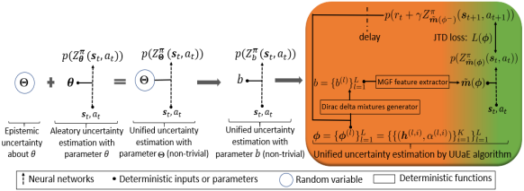
This section describes our proposed approach, called Unified Uncertainty-aware Exploration (UUaE), which is presented in Algorithm 1. UUaE comprises three main components: (1) a belief-based distributional RL scheme that integrates both aleatory and epistemic uncertainty, (2) an estimation method that learns the composite uncertainty, and (3) an exploration strategy that exploits the composite uncertainty for exploration.
4.1 Belief-based distributional RL
| Input: : size of GMM, : number of delta mixtures, : discount factor, : size of MGF features. |
| Initialize: : initial state, : parameters of previous belief, : parameters of current belief. |
| Take action , observe and . |
| Choose . |
| Compute . |
| Update as . |
| Update as |
To avoid the ambiguity of “the distribution of a random variable of a random variable ”, we represent epistemic uncertainty in the form of a belief distribution over a set of plausible parameters , i.e., . Assuming that for are distributed independently, we have , where . As the agent does not know the exact value of , it must be able to learn the return distribution from the belief . By defining and and by taking the expectation of Eq. (1) with respect to and , the so-called belief-based distributional Bellman equation is derived as
| (4) |
where
As parameters of reflect the belief over , we refer to as the belief-based return distribution. The derived belief-based distributional Bellman equation provides a basis for incorporating epistemic uncertainty into the aleatory uncertainty learning processes of current distributional RL methods.
4.2 Unified uncertainty estimation
Parameterizing directly with the belief is non-trivial. To feed as the parameters of to a network, we require to
extract sufficient features of . To that end, we first need to characterize . We begin by modelling as a mixture of Dirac deltas with parameters describing locations and weights of Dirac deltas.
To pivot the non-trivial belief-based return distribution estimation problem into a previously-solved return distribution estimation problem, which can be solved through Eq. (2), we introduce a feature extraction method for based on MGF of . MGF of a random variable is a computationally efficient alternative specification of its probability distribution [28]. The MGF of with belief for a fixed vector is given by . We represent with the feature vector , where is the -th order moment (-way tensor) of achieved from the -th order
derivative of the MGF at . Thus, the total features for are given in . Using Dirac deltas for modelling has several benefits: (1) A mixture of Dirac deltas can be considered as a GMM with zero (co)variances. Hence, like GMMs, a mixture of deltas can approximate any probability distribution by adjusting the number of mixtures [27]. (2) The MGF corresponding to a mixture of deltas exists on an open interval around , and higher-order moments of can be computed efficiently. (3) The moments of are differentiable with respect to ; thus, can be directly optimized via gradient descent during back-propagation.
Lastly, by substituting for in Eq. (4), we obtain:
| (6) |
To learn the parameter vector , we utilize a mixture density network [27] with a total parameter vector . Our network takes in as input and produces outputs , , and . The network must minimize the statistical distance between two GMMs: and . The Wasserstein distance and Kullback-Leibler divergence, which are commonly used in distributional RL literature [3, 8, 25], between two GMMs are analytically intractable. Thus, we utilize the recently proposed Jensen-Tsallis Distance (JTD) [27], which has a closed form between two GMMs and provides unbiased sample gradients. The gradient of the JTD loss function with respect to is calculated as a matrix multiplication between the gradient of the loss with respect to the network parameters and Jacobian matrix of the MGF-feature extractor function as
4.3 Composite uncertainty-aware exploration
Following common practices in RL [21, 24], we interpret the uncertainty of a random variable as its variance (or trace of its covariance). Thus, captures the epistemic uncertainty since , and the composite variance is the irreducible aleatory uncertainty with the parameter including epistemic uncertainty. Therefore, while attempting to maximize expected rewards , the agent should avoid regions with high aleatory uncertainty to avoid excessive risk-seeking behavior, i.e.,
Fig. 1 provides an illustration of uncertainty estimation in our proposed UUaE method.
5 EXPERIMENTS
In this section, we evaluate the performance of UUaE on two Atari games with sparse reward functions. To test the proposed algorithm in a more realistic setting, we also run our algorithm on an autonomous vehicle driving simulator [29] in a highway domain, where rewards are designed to penalize unsafe driving behavior. The sparsity and risk-sensitivity of rewards in these tasks make uncertainty-aware exploration challenging.
Baselines: We compare the performance of UUaE to three recently proposed algorithms: SUNRISE [9], DLTV [21], and IV-DQN [24], which respectively act based on the epistemic uncertainty, aleatory uncertainty, and additive formulation of epistemic and aleatory uncertainty.
Setup: We implement the baselines using their original implementations. The hyperparameters , , and of UUaE are empirically set to , , and . The experiments indicated a monotonic increase in performance with higher values of , , and . However, larger values of these hyperparameters lead to an increase in computation time. Thus, a trade-off between the computation time and performance must be made to choose these values.
Results: Following common approaches in RL literature [9, 21, 24], we measure the performance of algorithms in terms of the cumulative reward. Fig. 2 presents the results averaged over random seeds, with shaded areas indicating the standard deviation. Our algorithm outperforms all three baselines across all three environments, demonstrating the significance of our approach in integrating both aleatory and epistemic uncertainties for exploration and in the effectiveness of MGF features as a summary of the belief. Additionally, our method exhibits low variance and good risk-sensitive performance, making it more stable than the baselines. In the autonomous driving task, SUNRISE’s performance deteriorates substantially as it does not consider aleatory uncertainty, whereas driving safely on the highway necessitates risk-sensitive driving.
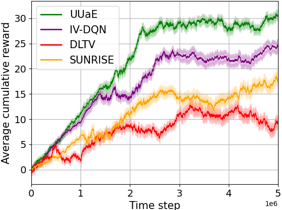
(a) Atari-Asterix
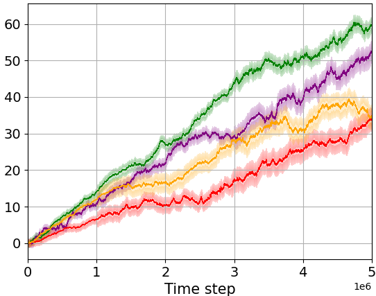
(b) Atari-Seaquest
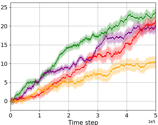
(c) Autonomous vehicle driving
6 Conclusion
Relying on a novel extension of the distributional RL to the so-called belief-based distributional RL, we provide a theoretical contribution for joint epistemic and aleatory uncertainty estimation. The proposed method scales up current distributional RL algorithms, which only consider aleatory uncertainty, to measure both sources of uncertainty. To efficiently explore environments with composite uncertainty, we approximate the belief as a mixture of Dirac deltas and extract features using MGFs. Our method outperforms recent alternatives and exhibits stable exploration in highly sparse and uncertain environments.
References
- [1] T. Yang, H. Tang, C. Bai, J. Liu, J. Hao, Z. Meng, and P. Liu, “Exploration in deep reinforcement learning: a comprehensive survey,” arXiv preprint arXiv:2109.06668, 2021.
- [2] O. Lockwood and M. Si, “A review of uncertainty for deep reinforcement learning,” arXiv preprint arXiv:2208.09052, 2022.
- [3] M. Chen, X. Xiao, W. Zhang, and X. Gao, “Efficient and stable information directed exploration for continuous reinforcement learning,” in ICASSP 2022-2022 IEEE International Conference on Acoustics, Speech and Signal Processing (ICASSP). IEEE, 2022, pp. 4023–4027.
- [4] T. M. Moerland, J. Broekens, and C. M. Jonker, “Efficient exploration with double uncertain value networks,” arXiv preprint arXiv:1711.10789, 2017.
- [5] A. Campbell, L. Qendro, P. Liò, and C. Mascolo, “Robust and efficient uncertainty aware biosignal classification via early exit ensembles,” in ICASSP 2022-2022 IEEE International Conference on Acoustics, Speech and Signal Processing (ICASSP). IEEE, 2022, pp. 3998–4002.
- [6] H. Fang, T. Peer, S. Wermter, and T. Gerkmann, “Integrating statistical uncertainty into neural network-based speech enhancement,” in ICASSP 2022-2022 IEEE International Conference on Acoustics, Speech and Signal Processing (ICASSP). IEEE, 2022, pp. 386–390.
- [7] W. Dabney, M. Rowland, M. Bellemare, and R. Munos, “Distributional reinforcement learning with quantile regression,” in Proceedings of the AAAI Conference on Artificial Intelligence, 2018, vol. 32.
- [8] W. Dabney, Z. Kurth-Nelson, N. Uchida, C. K. Starkweather, D. Hassabis, R. Munos, and M. Botvinick, “A distributional code for value in dopamine-based reinforcement learning,” Nature, vol. 577, no. 7792, pp. 671–675, 2020.
- [9] K. Lee, M. Laskin, A. Srinivas, and P. Abbeel, “Sunrise: A simple unified framework for ensemble learning in deep reinforcement learning,” in International Conference on Machine Learning. PMLR, 2021, pp. 6131–6141.
- [10] S. Lee, Y. Seo, K. Lee, P. Abbeel, and J. Shin, “Offline-to-online reinforcement learning via balanced replay and pessimistic q-ensemble,” in Conference on Robot Learning. PMLR, 2022, pp. 1702–1712.
- [11] C. Bai, L. Wang, Z. Yang, Z. Deng, A. Garg, P. Liu, and Z. Wang, “Pessimistic bootstrapping for uncertainty-driven offline reinforcement learning,” arXiv preprint arXiv:2202.11566, 2022.
- [12] T. Hiraoka, T. Imagawa, T. Hashimoto, T. Onishi, and Y. Tsuruoka, “Dropout q-functions for doubly efficient reinforcement learning,” in International Conference on Learning Representations, 2022.
- [13] Y. Wu, S. Zhai, N. Srivastava, J. Susskind, J. Zhang, R. Salakhutdinov, and H. Goh, “Uncertainty weighted actor-critic for offline reinforcement learning,” arXiv preprint arXiv:2105.08140, 2021.
- [14] M. Turchetta, A. Krause, and S. Trimpe, “Robust model-free reinforcement learning with multi-objective bayesian optimization,” in 2020 IEEE International Conference on Robotics and Automation (ICRA). IEEE, 2020, pp. 10702–10708.
- [15] P. Malekzadeh, M. Salimibeni, A. Mohammadi, A. Assa, and K. N. Plataniotis, “Mm-ktd: multiple model kalman temporal differences for reinforcement learning,” IEEE Access, vol. 8, pp. 128716–128729, 2020.
- [16] M. Salimibeni, P. Malekzadeh, A. Mohammadi, and K. N. Plataniotis, “Distributed hybrid kalman temporal differences for reinforcement learning,” in 2020 54th Asilomar Conference on Signals, Systems, and Computers. IEEE, 2020, pp. 579–583.
- [17] Y. Tang and S. Agrawal, “Exploration by distributional reinforcement learning,” arXiv preprint arXiv:1805.01907, 2018.
- [18] R. Keramati, C. Dann, A. Tamkin, and E. Brunskill, “Being optimistic to be conservative: Quickly learning a cvar policy,” in Proceedings of the AAAI Conference on Artificial Intelligence, 2020, vol. 34, pp. 4436–4443.
- [19] P. Clavier, S. Allassonière, and E. L. Pennec, “Robust reinforcement learning with distributional risk-averse formulation,” arXiv preprint arXiv:2206.06841, 2022.
- [20] A. Mavor-Parker, K. Young, C. Barry, and L. Griffin, “How to stay curious while avoiding noisy tvs using aleatoric uncertainty estimation,” in International Conference on Machine Learning. PMLR, 2022, pp. 15220–15240.
- [21] B. Mavrin, H. Yao, L. Kong, K. Wu, and Y. Yu, “Distributional reinforcement learning for efficient exploration,” in International conference on machine learning. PMLR, 2019, pp. 4424–4434.
- [22] H. Eriksson, D. Basu, M. Alibeigi, and C. Dimitrakakis, “Sentinel: taming uncertainty with ensemble based distributional reinforcement learning,” in Uncertainty in Artificial Intelligence. PMLR, 2022, pp. 631–640.
- [23] W. R. Clements, B. Van Delft, B.-M. Robaglia, R. B. Slaoui, and S. Toth, “Estimating risk and uncertainty in deep reinforcement learning,” arXiv preprint arXiv:1905.09638, 2019.
- [24] V. Mai, K. Mani, and L. Paull, “Sample efficient deep reinforcement learning via uncertainty estimation,” arXiv preprint arXiv:2201.01666, 2022.
- [25] N. Nikolov, J. Kirschner, F. Berkenkamp, and A. Krause, “Information-directed exploration for deep reinforcement learning,” in International Conference on Learning Representations, 2019.
- [26] M. G. Bellemare, W. Dabney, and R. Munos, “A distributional perspective on reinforcement learning,” in International Conference on Machine Learning. PMLR, 2017, pp. 449–458.
- [27] Y. Choi, K. Lee, and S. Oh, “Distributional deep reinforcement learning with a mixture of gaussians,” in 2019 International Conference on Robotics and Automation (ICRA). IEEE, 2019, pp. 9791–9797.
- [28] R. A. Johnson and G. K. Bhattacharyya, Statistics: principles and methods, John Wiley & Sons, 2019.
- [29] E. Leurent, “An environment for autonomous driving decision-making,” GitHub, 2018.