Lift-Connected Surface Codes

Abstract

We use the recently introduced lifted product to construct a family of Quantum Low Density Parity Check Codes (QLDPC codes). The codes we obtain can be viewed as stacks of surface codes that are interconnected, leading to the name lift-connected surface (LCS) codes. LCS codes offer a wide range of parameters - a particularly striking feature is that they show interesting properties that are favorable compared to the standard surface code already at moderate numbers of physical qubits in the order of tens. We present and analyze the construction and provide numerical simulation results for the logical error rate under code capacity and phenomenological noise. These results show that LCS codes attain thresholds that are comparable to corresponding (non-connected) copies of surface codes, while the logical error rate can be orders of magnitude lower, even for representatives with the same parameters. This provides a code family showing the potential of modern product constructions at already small qubit numbers. Their amenability to 3D-local connectivity renders them particularly relevant for near-term implementations.

I Introduction

Quantum Error Correcting (QEC) codes are essential for the reliable operation of quantum computers [1]. Recent advances in hardware quality and qubit count of quantum computing devices enabled first experiments realizing different aspects of quantum error correction [2, 3, 4, 5, 6, 7].

QEC codes encode logical qubits in a subspace of a higher dimensional Hilbert space. For stabilizer codes, the codespace is spanned by the simultaneous $+1$-eigenspace of a set of commuting operators, the stabilizer generators. The commonly shown parameter triple $[[n,k,d]]$ denotes the number of physical qubits $n$ employed by the error correcting code to encode $k$ logical qubits with a minimum distance $d$. The latter is defined as the minimum number of single qubit Pauli operators that have non-trivial action on the codespace, i.e. the minimum weight of a logical operator. A code with distance $d$ can correct at least for all errors up to weight $t=\frac{d-1}{2}$. A code family is specified by a sequence of stabilizer codes (that share most properties) with growing number of physical qubits. Promising QEC code families are surface codes [8]. Surface codes only require nearest neighbor connectivity in a planar 2D architecture. This makes them especially suited for experimental platforms with manifest connectivity constraints, such as superconducting qubits. Additionally, surface codes have some of the highest known thresholds for realistic circuit level noise models [9, 10].

Despite these strong upsides, a major shortcoming of surface codes is the observation that a surface code patch essentially always encodes only a single logical qubit irrespective of the size of the patch. This is captured by the so-called code rate $r=\frac{k}{n}$, i.e. the ratio of logical to physical qubit numbers, which is asymptotically zero for the surface code. In practical terms, this implies that scaling the code to improve its correction capabilities leads to a substantial qubit overhead. This in turn defines the challenge to find codes with better encoding rate while giving up as little as possible with respect to connectivity and logical (threshold) performance. To highlight a result in this direction, it has been shown that codes with bounded connectivity attaining a constant encoding rate could be used for constant overhead fault-tolerant quantum computation [11]. Codes built from stabilizers with bounded degree of connectivity are called quantum low-density parity check codes (QLDPC). In particular, a $(d_{q},d_{s})$-QLDPC family of codes $\mathcal{Q}_{i}$ with $n_{i}\to\infty$ as $i\to\infty$ has every qubit involved in a maximum of $d_{q}$ stabilizer measurements and every stabilizer measurement involving at most $d_{s}$ qubits, independent of $i$ [12]. A (Q)LDPC code family with both an asymptotically constant rate and a linear distance scaling, i.e. $[[n,k\propto n,d\propto n]]$, is called ”good”. For a recent overview of QLDPC codes see [13].

The definition of QLDPC captures the bounded connectivity found in the surface (or closely related toric) and color codes. However despite technically being QLDPC, these are far from ”good” both due to their vanishing rate and moreover their sub-optimal distance scaling $d\propto\sqrt{n}$. A big leap towards QLDPC codes with improved scalings was provided by the invention of the hypergraph product construction [14]. Here, the product of two classical codes gives a quantum code, which remarkably preserves the (Q)LDPC property provided the two classical codes are LDPC to begin with. With this construction, the product of two good classical codes leads to a QLDPC code with constant rate while maintaining the distance scaling of the surface code ($d\propto\sqrt{n}$) [15, 14]. After a series of breakthroughs, this line of research of product code constructions recently culminated in the remarkable discovery of good QLDPC codes, i.e. quantum codes with constant rate and linear distance [16, 17]. Additional constructions of good QLDPC code families followed shortly after [18, 19].

These results establish QLDPC codes as promising candidates for fault-tolerant quantum computation. By the same token, they define substantial challenges, both on the experimental and on the theory side. As a first challenge, known constructions of good codes involve prohibitively large numbers of qubits ($\sim 10^{6}$), leaving a substantial gap between what will be realistically available in near-term devices and what would be required for the above. As a second challenge, good QLDPC codes have been proven to require geometrically non-local connectivity. In fact, no-go theorems prevent good scaling of parameters if the connectivity of the code is restricted to some neighborhood that does not grow with the code [20, 21]. Several proposals on circuit constructions and implementation of QLDPC codes with constrained connectivity in mind have been formulated [22, 23, 24] and code constructions that explicitly leverage hardware capabilities like modularity are also considered [25]. Progress in platforms that allow for more connectivity opens the road to implement more advanced codes. Ion traps achieve all-to-all connectivity in single crystals mediated by motional modes, limited to a few tens of qubits [26]. This restriction can be overcome by the ability to shuttle ions [27]. Shuttling also enables effective all-to-all connectivity in neutral atom arrays, where coherent control of hundreds of atoms can be realized [28, 29, 30, 31, 32, 33]. The potential for quantum error correction in neutral atom quantum processors has very recently been demonstrated in Ref. [7].

Further challenges from the conceptual side are logical gates and decoding. Decoders adapted from classical coding theory like Belief Propagation and Ordered Statistics Decoding (BP+OSD) perform reasonably well, but symmetry of certain quantum codes and large distances pose ongoing challenges [34, 35, 36, 37]. While efficient decoders for good QLDPC codes are in principle available, the lack of codes with reasonable size prevents benchmarking these codes [38, 39, 19]. Additionally, QLDPC codes with a property known as single-shotness allow for fault-tolerance with only a single round of (noisy) syndrome measurement, but at the cost of a large qubit overhead [40, 41].

Fault-tolerant implementations of logical gates like transversal, i.e. single qubit decomposable gates, in general rely on symmetries of the code [42, 43, 44]. Several approaches for general codes include teleportation based gates [45], generalized lattice surgery [46] or codes specifically constructed to support certain gates [47]. For hypergraph product codes, some implementations of gates have been proposed, but they remain short of generality or practicality [48, 49].

I.1 Summary of Results

In this work, we introduce a new QLDPC code family, which we call lift-connected surface (LCS) codes. For their construction, we employ the recently established lifted product. This technique is a key ingredient in the recent groundbreaking discovery of good QLDPC codes. Using comparatively simple input codes, we obtain QLDPC codes that can be straightforwardly seen as sparsely interconnected copies of surface codes, leading to the name LCS. While their asymptotic scaling is not ”good” in the strict sense of the term, i.e. in a constant rate regime, the distance grows proportional to the physical qubit number up to a maximum size (see discussion around Eq. 16), they demonstrate the near-term potential of QLDPC (specifically lifted product) codes. We benchmark LCS codes under code capacity as well as phenomenological noise (i.e. noisy syndrome measurements) using an adapted BP+OSD decoder. We find that their asymptotic thresholds are comparable to disjoint copies of surface codes, summarized in Tab 1. However for concrete realizations they offer substantially lower logical error rates and higher pseudo-thresholds. Given that these advantages already appear for as few as tens of qubits, these results are promising for near-term QEC experiments.

Table 1: Bit-flip noise thresholds of LCS codes compared to copies of surface codes, obtained from BP+OSD decoding of codes with increasing distance. For details of the families, refer to the text. All uncertainties here and in the following are readoff errors.

Code	threshold
	code capacity	phenomenological
LCS code family 1	$6.7\pm 0.3\%$	$2.9\pm 0.1\%$
LCS code family 2	$7.7\pm 0.2\%$	$3.2\pm 0.1\%$
$d$ copies of distance $d$ surface codes	$7.5\pm 0.3\%$	$2.9\pm 0.1\%$

The manuscript is structured as follows. In Sec. II, we review the lifted product construction for quantum error correcting codes. In Sec. III, we show how LCS codes are constructed from the lifted product and describe the code parameters and structure. In Sec. IV we perform simulations over code capacity and phenomenological noise channels for several members of the LCS family, showing their error correction capabilities. Finally we outline a path towards logical gates in LCS codes in Sec. V before concluding in Sec. VI.

II The Lifted Product Construction

The lifted product (LP) construction combines classical LDPC codes based on circulant permutation matrices with the hypergraph product (HGP) construction for quantum codes [50, 14].

II.1 Hypergraph Product

A parity check matrix of a (classical code) $H$ can be represented by the so-called Tanner graph by identifying its rows (the parity checks $c$) with one type of node and its columns (the (qu)-bits $q$) with another type of node. An edge between nodes is drawn whenever the corresponding entry $H_{cq}$ is 1, making the graph manifestly bipartite [51]. Let $\mathcal{T}_{\mathcal{C}_{1}}$ and $\mathcal{T}_{\mathcal{C}_{2}}$ be the Tanner graphs of two classical codes $\mathcal{C}_{1}$ and $\mathcal{C}_{2}$ with binary parity check matrices $H_{1}\in\mathbb{F}_{2}^{m_{1}\times n_{1}},H_{2}\in\mathbb{F}_{2}^{m_{2}\times n_{2}}$ respectively. We will sometimes refer to these as base matrices. The Tanner graph of the hypergraph product (quantum) code $\mathcal{T}_{\mathcal{Q}}$ is based on the Cartesian product of the classical Tanner graphs $\mathcal{T}_{\mathcal{C}_{1}}$ and $\mathcal{T}_{\mathcal{C}_{2}}$. A graphical construction is shown in Fig. 1, for details refer to Ref. [14]. Here, we review the algebraic construction rule when given two base matrices. The parity check matrices of the hypergraph product quantum CSS code are given by

The CSS commutativity constraint $H_{Z}H_{X}^{T}=0$ is fulfilled by construction since

(1)

(2)

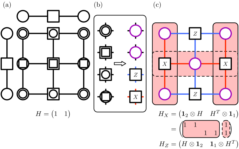
Figure 1: Pictorial representation of the hypergraph product (HGP) construction. (a) Shows the Cartesian product of two repetition codes of length two with parity check matrix $H$. Black circles represent bits and black squares represent parity checks. With the prescription of (b), the Tanner graph (c) is obtained, which can be identified with the non-rotated $[[5,1,2]]$ surface code. Purple circles represent qubits, stabilizers are again black squares, where the edge color red (blue) denotes the Pauli-type $X$ ($Z$). We furthermore highlight the $X$-part as a guide to the reader to identify the blocks of the algebraic construction. The vertical stripes (solid border) correspond to the left $\mathbf{1}_{2}\otimes H$ part of $H_{X}$ as two copies of the original repetition code. The horizontal stripe (dashed border) comes from the right $H^{T}\otimes\mathbf{1}_{1}$ block, corresponding to (one copy of) the Tanner graph of the transposed repetition code.

Any choice of binary matrices $H_{1},H_{2}$ gives a valid quantum code. Notably, surface codes can be obtained from taking the HGP of the $\ell\times\ell+1$ parity check matrices of (classical) repetition codes, i.e.

The resulting surface code $\mathrm{HGP}(H^{(\ell)},H^{(\ell)})$ then has parameters $[[n,k,d]]=[[(\ell+1)^{2}+\ell^{2},1,\ell+1]]$.

If the base matrices are members of a good classical LDPC code family with parameters $[n_{\mathrm{cl}},k_{\mathrm{cl}}\propto n_{\mathrm{cl}},d_{\mathrm{cl}}\propto n_{\mathrm{cl}}]$, then the resulting HGP codes have constant rate and distance $d=\Omega(\sqrt{n})$ [14].

II.2 Lifted Product

To present the lifted product (LP) construction, we will follow the approach by Panteleev and Kalachev [50]. For a complementary approach see Ref. [13]. We restrict ourselves to a subset of LP codes, originally referred to as quasi-cyclic generalized hypergraph product codes [34]. We first briefly review this generalization, before carefully explaining the implications for our construction in the next section.

A useful starting point before attempting to go beyond the HGP is to note a subtle requirement in fulfilling the CSS commutativity constraint of Eq. 2. Given the two parity check matrices $H_{1}$ and $H_{2}$ and using Dirac notation, it is indeed true that

$$(H_{1}\otimes\mathbf{1}_{n_{2}})(\mathbf{1}_{n_{1}}\otimes H^{T}_{2})=$$ (3)

$$=\sum_{abgh}H_{1,ab}H^{T}_{2,gh}\outerproduct{ag}{bh}$$ (4)

$$=H_{1}\otimes H^{T}_{2},$$ (5)

however when doing the analogous calculation

$$(\mathbf{1}_{m_{1}}\otimes H^{T}_{2})(H_{1}\otimes\mathbf{1}_{m_{2}}) =\sum_{cgaf}H^{T}_{2,cg}H_{1,af}\outerproduct{ac}{fg},$$ (6)

the conclusion that this is also $H_{1}\otimes H^{T}_{2}$ rested on the assumption that all $H^{T}_{2,cg}$ and $H_{1,af}$ commute. While this commutativity is trivially true when the entries are numbers, it turns into a non-trivial requirement as soon as we want to promote the entries to higher-dimensional objects, e.g. matrices. In turn, this suggests that as long as we fulfill commutativity on this level, it will imply the fulfillment of the CSS constraint. One choice are elements of a commutative (matrix) ring, like circulant matrices of size $L\times L$. A circulant $C$ can be represented as sums of cyclic permutations $P^{(i)}$,

$$C=\sum_{i=0}^{L-1}c_{i}P^{(i)}$$ (7)

where $c_{i}$ are binary coefficients and $P^{(i)}$ denotes the $i^{\mathrm{th}}$ cyclic (right) shift. We denote $P^{(0)}$ by $I$. For any circulant, we can give a binary representation such that $\mathcal{B}_{L}(P^{(i)})$ is the $i^{\mathrm{th}}$ cyclic (right) shift of the identity matrix $\mathbf{1}_{L}$. For example

The LP construction then takes the HGP of two matrices with circulants as entries and replaces these with the corresponding binary representations after having taken the product. This increases the number of qubits and parity checks by a factor of $L$, which gives the procedure its name lifting. Denoting matrices with circulant entries with a tilde, an LP code is obtained as

(8)

Note that the transpose of a matrix with circulant entries $\tilde{A}=(a_{ij})_{m\times n}$ is $\tilde{A}^{T}=(a^{T}_{ji})_{n\times m}$ and it holds that $\mathcal{B}_{L}(\tilde{A}^{T})=\mathcal{B}_{L}(\tilde{A})^{T}$.

In graph-theoretical terminology, the parity check matrices $H_{X}$ and $H_{Z}$ are the biadjacency matrices of the Tanner graphs. We show the lifting procedure for the example Eq. LABEL:eqn:ex_lift_1 in Fig. 2. One edge of a Tanner graph of a HGP code with parity check matrix $H$ between check $c_{i}$ and qubit $q_{j}$ is shown in Fig. 2(a). In the LP construction, the entries of the final parity check matrix are replaced by circulants. This can be visualized by labelling the corresponding edge in the Tanner graph, as shown in Fig. 2(b). The lift, in Fig. 2(c) with lift parameter $L=4$, translates to copying the check and qubit nodes $L$ times and connecting them according to the non-zero entries of the circulant. In this example, the circulant $I+P^{(1)}$ connects every copy of the check $(c_{i},k)$ with two copies of qubits, $(q_{j},k)$ and $(q_{j},k+1\mod L)$.

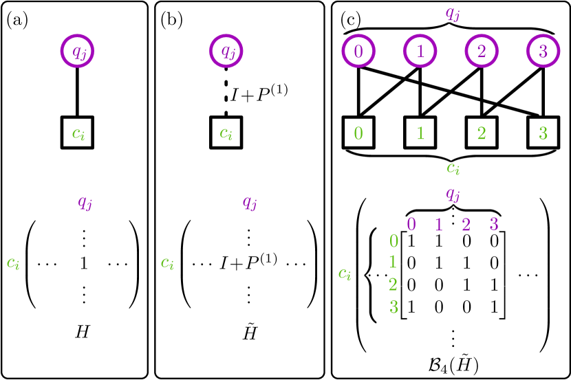
Figure 2: Lifting of edges of a graph that are part of the Tanner graph of a (quantum) code. (a) A nonzero entry of the parity check matrix $H_{ij}$ corresponds to an edge between check $c_{i}$ and qubit $q_{j}$. (b) A circulant entry like $I+P^{(1)}$ of a LP parity check matrix can be visualized by a label on the edge and a corresponding edge style. (c) The lift of the matrix corresponds to taking $L$ (here $L=4$) copies of the check and qubit nodes. The new connectivity is according to the binary representation of the circulant. In this example, the circulant $I+P^{(1)}$ connects every copy of the check $(c_{i},k)$ with two copies of qubits, $(q_{j},k)$ and $(q_{j},k+1\mod L)$.

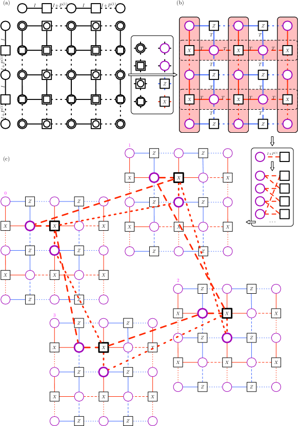
Figure 3: Pictorial representation of the lifted product construction for LCS codes with $(\ell,L)=(2,4)$. (a) First, we take the hypergraph product (HGP) of two repetition codes of length 3. The edges of the input Tanner graphs (top row and leftmost column) are now decorated and labeled to indicate that the scalar entries of the repetition code are being promoted (i.e. lifted) to matrices $I$ (solid) and $I+P^{(1)}$ (dashed) respectively, which are both of dimension $L\times L$. This label carries through to the resulting Tanner graph. (b) Analogously to the HGP, vertices are respectively identified with qubits, $X$- and $Z$-checks. The edge label again indicates whether the corresponding entries are taken from the identity matrix $I$ (solid) or the circulant $I+P^{(1)}$ (dashed). To obtain the stabilizers from this picture, first of all observe that since all edges contain the $I$ matrix, we will obtain $L$ copies of the code that we would have obtained without lifting. The non-trivial extension comes from the edges containing the additional term $P^{(1)}$, which define the additional entries in the resulting stabilizer checks between the different copies. Also note that the edges of the transposed base graphs (indicated by $T$) also have to be lifted by the transposed circulant. This is exemplarily spelled out in (c), where we show how the dashed edges of the given $X-$check in the LP are promoted to four $X-$checks on four copies of the underlying code and additional interconnections in the respective checks arise from the non-trivial circulants $P^{(1)}$ ($P^{(1)T}$). Note that the interconnections are highly structured, in particular they exclusively appear between neighboring code copies.

III The Lift-Connected Surface Codes

III.1 Construction and Parameters

We can use the LP construction to algebraically build copies of the (non-rotated) surface code. To that end, we take base matrices of size $\ell\times(\ell+1)$ of the same repetition code form as in Eq. II.1. The binary entries are replaced the trivial circulant ($P^{(0)}=I$) of size $L$ and zero circulant. The resulting matrix with circulant entries is denoted by $\tilde{H}^{(\ell)}$. Then the LP quantum code $\mathrm{LP}_{L}(\tilde{H}^{(\ell)},\tilde{H}^{(\ell)})$ consists of $L$ disjoint copies of distance $d=\ell+1$ surface codes. The parameters of the code are therefore

$$[[n,k,d]] =[[((\ell+1)^{2}+\ell^{2})L,L,\ell+1]],$$

$$(d_{q},d_{s}) =(4,4).$$ (9)

This insight can be used to construct interconnected surface codes. Consider matrices of size $\ell\times\ell+1$ with

(10)

The parity check matrices resulting from the first step (HGP) then naturally split into two parts,

(11)

(12)

The first addends $\tilde{H}_{X,\text{surface}},\tilde{H}_{Z,\text{surface}}$ have the same structure as surface codes. The lift therefore generates $L$ copies of surface codes. The second addends $\tilde{H}_{X,\text{interconnection}},\tilde{H}_{Z,\text{interconnection}}$ act as additional connections in between the surface code patches. We therefore call the codes $\mathrm{LP}_{L}(\tilde{H}^{(\ell)},\tilde{H}^{(\ell)})$ the $(\ell,L)$-lift-connected surface codes or simply LCS codes. The interconnections amount to at most two additional connections per check, because $\tilde{H}^{(\ell)}_{\text{int.}}$ contains at most one entry per row and column. The general form of the parity-check matrices is shown in App. A. The LCS code construction is shown pictorially in Fig. 3.

The LCS codes are therefore $(6,6)$-QLDPC. The dimension of a quantum CSS code is given by

$$k =n-\rank(H_{X})-\rank(H_{Z}).$$ (13)

Since both $H_{X}$ and $H_{Z}$ are already in a row echelon form and contain no zero rows, they are full rank and

$$k=((\ell+1)^{2}+\ell^{2})L-2\ell(\ell+1)L=L.$$ (14)

There is no general recipe to get the distance of LP codes from the ingredients of the construction [50]. We can, however, calculate it via brute force by searching through all stabiliser equivalent representatives of logical operators or bound the minimum distance by probabilistic methods using the GAP package QDistRnd [52]. We find for parameters $(\ell=1,L<100),(\ell=2,L<10),(\ell=3,L<5)$ that

$$d=\min(L,2\ell+1).$$ (15)

All data shown in this manuscript support this conjecture. In App. A, we show a constructive approach to establishing the minimum distance based on the block structure of the parity check matrices. In summary, the parameters of the LCS codes are

$$[[n,k,d]] =[[((\ell+1)^{2}+\ell^{2})L,L,\min(L,2\ell+1)]],$$

$$(d_{q},d_{s}) =(6,6).$$ (16)

Available codes are shown in Fig. 4 and discussed in the following section. When unclear, we denote the construction parameters as a superscript $[[n,k,d]]^{(\ell,L)}$. Note that for fixed $\ell$ and varying lift-parameter $L\leq 2\ell+1$, both the number of encoded logical qubits and the distance scale linearly in the number of physical qubits with constant rate $r=(2\ell^{2}+2\ell+1)^{-1}$.

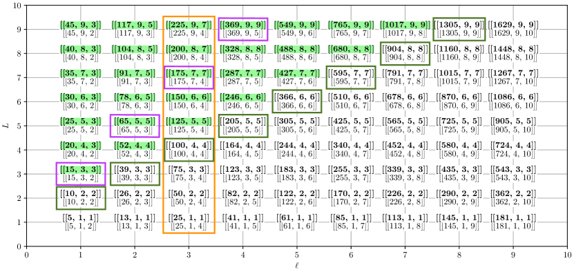
Figure 4: Code parameters $[[n,k,d]]$ of LCS (top, bold font) and copies of surface codes (bottom) for different $(\ell,L)$. The codes marked in dark green correspond to $L=\ell+1$ where both surface and LCS codes have the same parameters (family 1). Above that line for fixed $(\ell,L)$, the LCS codes have a larger distance compared to the copies of surface codes, indicated by the green shade behind the corresponding parameters. The purple boxes mark LCS code family 2 where for a fixed rate, codes with maximum distance and minimum number of physical qubits are chosen. The orange box ($\ell=\mathrm{const.}$) shows how for the LCS codes, $k,d$ scale linearly in $n$ up until $L=2\ell+1$.

III.2 Connectivity

Firstly, the LCS codes are QLDPC with $(d_{q},d_{s})_{\mathrm{lcs}}=(6,6)$ being slightly larger than the surface codes’ $(d_{q},d_{s})_{\mathrm{s}}=(4,4)$. The additional connectivity however is limited and indeed 3D-local. We label qubits with the tuple $(q_{i},s)$ where qubit $q_{i},i\in\{0,1,\dots,(\ell+1)^{2}+\ell^{2}-1\}$ of patch $s\in\{0,1,\dots L-1\}$ (and checks correspondingly with $(c_{i},s)$). An edge then is the tuple $e=[(c_{i},s),(q_{j},s^{\prime})]$. The circulant $P^{(1)}$ in the interconnection part of the parity check matrices interconnects only neighboring patches $s$ and $s+1\mod L$. The transposed circulant $P^{(1)T}=P^{(L-1)}$ turns the cyclic right shift by one into a cyclic left shift by one, keeping the restricted connectivity by only interconnecting neighboring patches $s$ and $s-1\mod L$. Hence, there only exist edges $e=[(c_{i},s),(q_{j},s^{\prime})]$ with $s^{\prime}=s+1\mod L$. Also, for every edge $e=[(c_{i},s),(q_{j},s^{\prime})]$ with $s\neq s^{\prime}$ there exists an edge $e=[(c_{i},s),(q_{j},s)]$, i.e. interconnection only involve checks and qubits that would have been connected within one patch. An example for $(\ell,L)=(2,5)$ is shown in Fig. 5, where the underlying surface codes are arranged as slices of a torus. Only a few interconnections are shown, but these have a bounded length. These observations imply that these codes might be suitable, e.g., for implementation in static 3D Rydberg atom array structures [53], without the need for shuttling. This only holds if the qubits at the outer edge are close enough to the respective ancillary qubit of the neighboring slice to perform entangling gates for stabilizer measurements. Concrete implementations and optimizations of qubit positions in 3D space are left as future work.

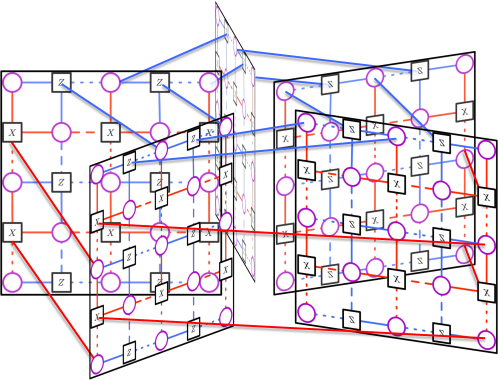
Figure 5: Possible arrangement of qubits of the $[[65,5,5]]^{(2,5)}$ LCS code, corresponding to $5$ interconnected $[[13,1,3]]$ surface codes. While only a few interconnections of the patches are shown, note that all connectivity is restricted to neighbors of neighboring patches and therefore 3D-local.

IV Code Performance over noisy quantum channels

IV.1 Sampling codes in quantum channels

Here we discuss several standard methods for (Monte Carlo) sampling of the combination of a given decoder and a noise model. We consider two types of noise models:

• Code capacity model: Only the data qubits are affected by a single qubit i.i.d. noisy quantum channel (e.g. a bit-flip channel). The syndrome measurement is assumed to be perfect, see also Alg. 1.

• Phenomenological noise model: This noise model extends the code capacity model by additionally including noisy syndrome measurements. This can e.g. be modeled by a perfect measurement followed by a (classical) bit-flip channel on the result, see Alg. 2.

Typically, to ensure a fault-tolerance level of $t=\frac{d-1}{2}$, the number of noisy error correction cycles is chosen to be $n_{\mathrm{ecc}}=d$. This assumes that with a maximum of $t$ noisy syndrome measurements, a majority vote on $d=2t+1$ noisy syndrome measurements allows one to more reliably choose a correction to apply. We can also think of this as defining repetition codes on the syndrome measurement outcomes, with extra variables introduced to model syndrome flips. In order to preserve the distance $d$ of the code, the length of these repetition codes is chosen to be $d$. This procedure is also shown in Fig. 6 for a three-bit repetition code.

IV.2 Decoding

A decoder takes syndrome data and potentially parameters of the noise model as input and returns an inference of the underlying error configuration (which in turn determines the appropriate recovery operation), that is consistent with the observed syndrome. Based on this error guess, a correction is applied that puts the state back to the codespace. The ideal maximum likelihood decoder picks a guess from the most likely error class, taking into account the code degeneracy, i.e. that distinct error configurations can be logically equivalent. Because this is in general computationally hard, practical decoders return an approximation, trading computational efficiency for non-optimality of the suggested recovery operation. E.g. the Most Likely Error (MLE) decoder tries to determine the most likely error configuration, ignoring potential degeneracies. To be efficient, practical decoders generally try to exploit structure in the code and noise model, such that not every existing decoder is suitable for application to a general code. Notably, a matching-based decoder like minimum weight perfect matching works well whenever elementary errors violate two parity checks [54]. This is not the case for LCS codes, since here a single error on a qubit violates up to $3$ parity checks (considering only $X$- and $Z$- errors). We therefore resort to two general purpose decoders, namely a MLE decoder and a decoder based on Belief Propagation and Ordered Statistics Decoding (BP+OSD) [55, 34].

Given our codes are symmetric with respect to $X$- and $Z$, we consider one Pauli type only, e.g. (single qubit, i.i.d) bit-flips with probability $p$, for a performance benchmark of the codes. The probability of a fixed configuration $E=\{E_{q}\}_{q=0}^{n-1}$ of errors given an observed syndrome $\mathbf{s}$ is

$$p(E|\mathbf{s}) \propto\prod_{q=0}^{n-1}p(E_{q})\prod_{c=0}^{n_{c}-1}\delta(\langle E,S_{c}\rangle=s_{c})$$ (17)

$$=p^{w}(1-p)^{n-w}$$ (18)

$$\propto\quantity(\frac{p}{1-p})^{w},$$ (19)

where $w$ is the weight of the configuration $w=\absolutevalue{E}$. $S_{c}\in\mathcal{S}$ denotes the stabilizer $c$ and $s_{c}$ the bit $c$ of the observed syndrome $\mathbf{s}$. We write $\langle P,P^{\prime}\rangle$ with $P,P^{\prime}\in\mathcal{P}_{n}$ for the function that indicates commutation,

$$\langle P,P^{\prime}\rangle=\begin{cases}0\mbox{\quad if\quad}\commutator{P}{P^{\prime}}=0\\ 1\mbox{\quad if\quad}\anticommutator{P}{P^{\prime}}=0.\end{cases}$$ (20)

With that notation, the syndrome of error $E$ can be written as

$$\sigma(E)=(\langle E,S_{c}\rangle)_{c=0}^{n_{c}-1}.$$ (21)

IV.2.1 MLE Decoding with i.i.d. noise

For $p<0.5$ ($p>0.5$), the most likely error (MLE) is the one with the lowest (highest) weight $w$. Landahl et al. give an intuitive implementation of an MLE decoder for quantum codes which we follow here [56].

Code capacity noise

Considering pure bit-flip noise, we have one (error free) syndrome $\mathbf{s}_{Z}=\{s_{Z,c}\}_{c=0}^{n_{c}-1}$. Let $\mathbf{x}=\{x_{q}\}_{q=0}^{n-1}$ be the binary representation of the Pauli error. Then MLE decoding can be stated as the optimization problem

$$\min \sum_{q}x_{q}$$ (22)

subject to $$\bigoplus_{q\in\Gamma(c)}x_{q}=s_{Z,c}\qquad\forall c$$ (23)

$$\quad\mathrm{with}\quad x_{q}\in\mathrm{GF}(2)=\{0,1\}.$$ (24)

Here, $\Gamma(c)$ is the set of qubits involved in stabilizer measurement $c$ and $\oplus$ indicates addition modulo $2$. In words, this procedure states: minimize the weight of an error that is compatible with the syndrome. In vectorised form with $Z$-parity check matrix $H_{Z}$, this can be written as

$$\min\quad \mathbf{1}^{T}\mathbf{x}$$ (25)

subject to $$H_{Z}\mathbf{x}=\mathbf{s}\!\mod 2$$ (26)

$$\quad\mathrm{with}\quad \mathbf{x}\in\mathrm{GF}(2)^{n}=\{0,1\}^{n}.$$ (27)

Phenomenological noise

With multiple rounds of noisy syndrome measurements, data errors after time step $t$ are indicated by differences of syndrome bits from $t$ to $t+1$. We write

$$\Delta\mathbf{s}_{t}=\mathbf{s}_{t}-\mathbf{s}_{t-1}=\mathbf{s}_{t}+\mathbf{s}_{t-1}\mod 2\quad\forall t$$ (28)

with $\mathbf{s}_{t=0}\!:=\!\mathbf{0}$ for the observed syndrome measurement outcomes. We introduce $d$ data-error vectors $\mathbf{x}_{0},\dots\mathbf{x}_{d-1}\in\mathrm{GF}(2)^{n}$ and $d$ syndrome measurement-error vectors $\tilde{\mathbf{s}}_{0},\dots\tilde{\mathbf{s}}_{d-1}\in\mathrm{GF}(2)^{n_{c}}$ for $d$ noisy rounds of error correction. This allows one to formulate the MLE decoding optimization problem as

$$\min \sum_{t}\mathbf{1}^{T}\mathbf{x}_{t}$$ (29)

subject to $$H\mathbf{x}_{t}+\tilde{\mathbf{s}}_{t}+\tilde{\mathbf{s}}_{t-1}=\Delta\mathbf{s}_{t}\!\mod 2\quad\forall t,$$ (30)

requiring that the noise-less syndrome together with syndrome errors are compatible with the observed syndrome differences. A last round of perfect syndrome measurements allows us to verify the correction returned by the optimization (see App. 2). Vectorized, this reads

$$\min\quad \mathbf{1}^{T}\mathbf{y}$$ (31)

subject to $$A\mathbf{y}=\Delta\mathbf{s}\mod 2$$ (32)

$$\quad\mathrm{with}\quad\mathbf{y}=(\mathbf{x}_{0}^{T},\dots,\mathbf{x}_{d-1}^{T}, \tilde{\mathbf{s}}_{0}^{T},\dots\tilde{\mathbf{s}}_{d-1}^{T})\in\mathrm{GF}(2)^{2dn}.$$ (33)

Here

$$A=\left(\begin{array}[]{c|c}\matrixquantity{H&&&\\ &H&&\\ &&\ddots&\\ &&&H}&\matrixquantity{\begin{matrix}I\\ I&I\end{matrix}&&\\ &\ddots&\\ &&\begin{matrix}I&I\end{matrix}}.\end{array}\right)$$ (35)

We implement the MLE decoder in python using the optlang interface [57] to the GNU Linear Programming Kit GLPK [58] to solve the constrained minimization. The run-time of decoding is exponential in the number of qubits and (noisy) error correction rounds. In practice, this results in a limitation on the feasibility of simulating the decoding of codes. We restrict the simulations to codes with $nd\leq 250$.

IV.2.2 Belief Propagation + Ordered Statistics Decoding

To enable benchmarking beyond low qubit numbers, we employ Belief Propagation and Ordered Statistics Decoding (BP+OSD). Belief Propagation (BP) is a well known decoder for classical codes, where it works particularly well for good LDPC expander codes [59, 60]. BP calculates single-qubit error probabilities using statistical inference on the Tanner graph of the code. While BP can be shown to be exact on trees, Tanner graphs usually contain cycles, which can hinder the performance of BP (see e.g. Refs. [55, 61]). One way to overcome these problems is to use Ordered Statistics Decoding (OSD) as a post-processor. While BP may be inconclusive in its output, it usually points to a subset of likely erroneous qubits, OSD then brute-forces the solution of the decoding problem on that subset [34].

We denote the qubits participating in syndrome measurement $c$ by $\Gamma(c)\subset{Q}$ with $Q$ the set of all qubits. The syndrome measurements in which qubit $q$ participates are $\Gamma(q)$. To approximate single qubit marginal probabilities, two types of quantities, termed messages, are updated iteratively until convergence or a maximum number of iterations is reached. The messages $m_{q\to c}(E_{q})$ from qubit $q$ to check $c$ correspond to the current estimate of error probabilities for $E_{q}$ on qubit $q$ given the estimates of all neighboring checks except $c$,

$$\displaystyle m^{(i+1)}_{q\to c} \propto p_{0}(E_{q})\prod_{c^{\prime}\in\Gamma(q)\setminus c}m^{(i)}_{c^{\prime}\to q}(E_{q}).$$ (36)

The messages $m_{c\to q}(E_{q})$ from check $c$ to qubit $q$ collect incoming probability estimates of qubits except $q$ and sum over all compatible configurations fixing the error $E_{q}$,

$$m^{(i)}_{c\to q} \propto\sum_{E_{\Gamma(c)\setminus q}}\delta[\sigma(E)_{c}=s_{c}]\prod_{q^{\prime}\in\Gamma(c)\setminus q}m^{(i)}_{q^{\prime}\to c}(E_{q^{\prime}}).$$ (37)

The product of all these messages incoming at a qubit node gives an estimate for the marginal probabilities of errors on that qubit, called belief,

$$b_{q}(E_{q}) \propto p_{0}(E_{q})\prod_{c\in\Gamma(q)}m^{(i_{\text{max}})}_{c\to q}(E_{q}).$$ (38)

The log-likelihood ratios

$$l_{q} =\log\frac{1-b_{q}(E)}{b_{q}(E)}$$ (39)

of qubit $q$ are calculated and used to sort the qubits by their likelihood of being erroneous. In first order OSD, the parity check matrix $H$ is truncated to a full rank square matrix $H_{[R]}$, with $R\subseteq Q$ a set of qubits which are most likely to have an error based on the log-likelihood ratios. Here $H_{[R]}$ refers to a restriction of $H$ to the columns specified in the set $R$. The OSD decoder then assumes no error on the set of remaining qubits $Q\setminus R$ and inverts the truncated matrix to get as a total error guess (up to reordering of the qubits)

$$\mathbf{x}=(H^{-1}_{[R]}\mathbf{s},\mathbf{0}_{[Q\setminus R]}).$$ (40)

Higher-order OSD improves upon that by considering non-zero configurations $\mathbf{x}_{[Q\setminus R]}$ for the remaining qubits and adapting the reliable part to ensure validity as

$$\mathbf{x}=(H^{-1}_{[R]}\mathbf{s}+H^{-1}_{[R]}H_{[Q\setminus R]}\mathbf{x}_{[Q\setminus R]},\mathbf{x}_{[Q\setminus R]}).$$ (41)

BP+OSD provides a a general purpose decoder that is efficient enough for reasonable benchmarking and has a well tested implementation [35, 62, 63]. In App. B, we provide details on chosen parameters. For small qubit numbers, it is typically observed that the performance of BP+OSD comes close to most-likely error decoding, see App. C for a comparison.

As BP+OSD essentially provides a solution $\mathbf{x}$ to ${H\mathbf{x}=\mathbf{s}\mod 2}$, we can also use the same algorithm to find a solution to $A\mathbf{y}=\Delta\mathbf{s}\mod 2$ (Eq. 32) representing the phenomenological noise model. In the graphical picture, this corresponds to taking $d$ copies of the code’s Tanner graph, adding new variable nodes for every check and interconnecting them according to the right part of the matrix $A$. An example of the adapted Tanner graph for a $3$-bit repetition code using three rounds of noisy measurements is shown in Fig. 6. Note that also here, we simulate a final destructive single qubit readout by a round of noiseless syndrome measurement.

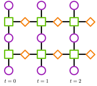
Figure 6: Phenomenological noise Tanner graph for a $3$-bit repetition code using $3$ rounds of noisy measurements. Newly introduced syndrome-error variables $\tilde{\mathbf{s}}$ are represented by orange rhombi. Note that this Tanner graph is (up to the rightmost rhombi) equivalent to the Tanner graph of a distance 3 surface code.

IV.3 Simulation Results

In the following section, we present results we obtain from sampling LCS codes for code capacity and phenomenological noise channels, which we compare to the performance of the standard surface code. Because LCS and surface codes are both CSS and $X$- and $Z$-stabilizers are symmetric up to permutations, it suffices to focus on pure bit-flip noise. We start with a discussion of the results for the smallest distance instances of LCS codes. We then move to larger codes, where we first discuss how to compare different finite rate codes and then present the core results regarding logical performance and thresholds of LCS codes.

IV.3.1 Logical error rate and pseudo-threshold

As we will be considering codes with more than one logical qubit, we will declare logical failure whenever any of the constituent logical qubits has an error. The logical error rate is given by

$$p_{\text{ler}} =\sum_{w=t+1}^{n}N_{\text{ler}}(w)p^{w}(1-p)^{n-w}$$ (42)

$$=(1-p)^{n}\sum_{w=t+1}^{n}N_{\text{ler}}(w)\quantity(\frac{p}{1-p})^{w},$$ (43)

where $N_{\text{ler}}(w)$ is the number of failure configurations of weight $w$ and $t=\frac{d-1}{2}$ is the minimum number of correctable errors. Let us start by looking at small LCS codes with $\ell=1$, $L\in\{3,4,5\}$ and parameters $[[15,3,3]],[[20,4,3]]$ and $[[25,5,3]]$ respectively with a rate of $r=1/5$. The first two codes are also shown in Fig. 12. The logical error rate against the physical error rate is shown in Fig. 9 $(a)$.

We make the following observations about the given distance $3$ codes: first of all, the different codes show a similar logical error rate across the range of physical error rates, where the logical error rate is larger for larger physical qubit number, as expected when fixing the distance. Furthermore the logical error rate scaling at low $p$ is consistent with $p_{\text{ler}}\propto p^{2}$, indicating that arbitrary single qubit errors are corrected. Remarkably, $3$ copies of distance $3$ surface codes with parameters $[[39,3,3]]$ have a logical error rate comparable to the $[[20,4,3]]$ LCS code encoding one logical qubit more with fewer physical qubits.

To further assess the performance of the error correcting codes, we can look at the physically motivated pseudo-threshold $p^{\star}_{\mathrm{th}}$ [64]. It is the value of physical error rate $p$ below which the logical error rate is lower than the physical error rate. In general, we call the presence of any faulty (logical) qubit in our computational (logical) Hilbert space a (logical) failure. This implies that for $k$ bare physical qubits each failing with $p$, their total failure probability is given by

$$p_{\text{fail}}(k) =\sum_{l=1}^{k}\binom{k}{l}(1-p)^{k-l}p^{l}$$ (44)

$$=1-(1-p)^{k}.$$ (45)

This reduces to the well known case for $k=1$, $p_{\text{fail}}=p$ that is often considered for (planar) color or surface codes hosting one logical qubit.

As shown in Fig. 9 $(a)$, The pseudo-thresholds are in the range of $8-9\%$.

IV.3.2 Logical error rate per logical qubit

In a practical setting, we can not distinguish which of the logical qubits has a logical error and therefore, any error is bad. Additionally, a rescaling of the logical error rate to a logical error rate per logical qubit in order to e.g. compare codes with a different number of logical qubits $k$ is only meaningful if they fail independently of each other. Fig. 7 shows the probability of logical errors in the $[[15,3,3]]$ code for a bit-flip error rate $p_{\mathrm{x}}=0.01$. Most notably, $p(X_{0}X_{1}X_{2})\neq p(X_{0})p(X_{1})p(X_{2})$ indicates that the logical qubits do not fail independently. This is in contrast to using multiple codes each encoding only a single logical qubit. We will therefore always consider the logical failure of the block as soon as any logical qubit comprising it fails. Whenever we compare to surface codes with $1$ logical qubit, we obtain the logical error rate for $k$ copies of surface codes by rescaling the single-logical qubit error rate as

$$p_{\mathrm{L}}^{(k)}=1-(1-p_{\mathrm{L}}^{(1)})^{k}.$$ (46)

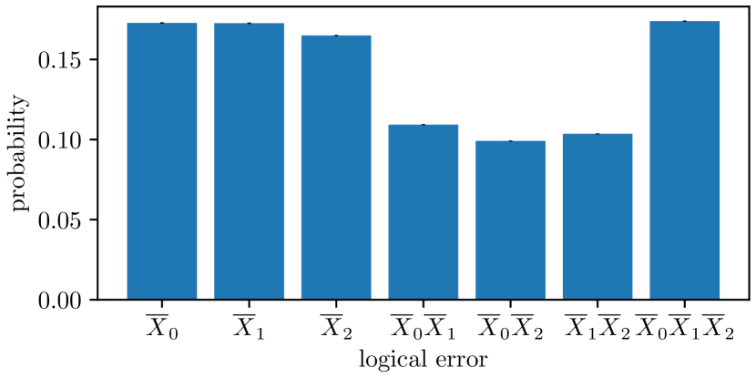
Figure 7: Probability of logical errors at $p_{\mathrm{x}}=0.01$ for the $[[15,3,3]]$ LCS code. The logical qubits don’t fail independently as $p(\overline{X}_{i})p(\overline{X}_{j})\neq p(\overline{X}_{i}\overline{X}_{j})$. Because of the symmetry of the code and the noise, we expect the same logical error rates for e.g. $\overline{X}_{0}$ and $\overline{X}_{2}$. We attribute the difference seen above to the specific implementation of the decoder that returns only one solution whenever there are multiple with the same likelihood.

IV.3.3 Copies of single-logical qubit codes or single-block codes?

In the following, we will discuss and compare logical error rates of various LCS and surface codes encoding the same number of logical qubits $k=3$ and distance $d=3$. This corresponds to $\ell\in\{1,2,3\}$, $L=3$. Fig. 9 $(b)$ shows the logical error rate of these codes sampled over a code capacity channel and decoded with the MLE decoder. For the interconnected $[[39,3,3]]]$ LCS codes, the logical error rate is almost an order of magnitude lower for small physical bit-flip rates $p_{\mathrm{x}}$ compared to three copies of $[[13,1,3]]$ surface codes. To explain this remember that at low $p$ the logical error rate is dominated by low-weight failure configurations. Using a look-up table decoder, we count the number of failure configurations, shown in Tab. 2 for a weight $w\leq 5$. The number of failure configurations is significantly lower for the LCS code encoding the $3$ logical qubits in one block which results in the significantly lower logical error rate. Also the pseudo-threshold is significantly higher with $p^{\star}_{\mathrm{th}}([[39,3,3]]-\text{LCS})\approx 8.6\%$ against $p^{\star}_{\mathrm{th}}(3\cdot[[13,1,3]]-\text{S})\approx 6.4\%$. Note that the codes with smaller encoding rate $r=\frac{k}{n}$ show a lower logical error rate, which is plausible given their correspondingly higher number of stabilizers. However, the $[[75,3,3]]$-LCS code only has a marginally lower logical error rate compared to the $[[39,3,3]]$-LCS code, hinting at a tradeoff between physical qubit number and degeneracy. Tab. 3 summarizes the pseudo-thresholds for these small codes, which are all in the range of $8-9\%$.

For phenomenological noise, we set the probability of a noisy syndrome measurement to $q=p_{\mathrm{x}}=:p$. We report a lower bound on the logical error rate per cycle by rescaling the total logical error rate after $n_{\mathrm{ecc}}$ cycles as

$$p_{\mathrm{L}}(p)\geq 1-\left(1-p_{\mathrm{L}}(n_{\mathrm{ecc}})\right)^{\frac{1}{n_{\mathrm{ecc}}}}.$$ (47)

This can then be compared to the failure probability of $k$ unencoded qubits to get the pseudo-threshold as a solution to $p_{\mathrm{L}}(p)=1-(1-p)^{k}$, shown for the MLE decoder and distance $3$ bounded LCS codes in Fig. 9. The pseudo-thresholds are summarized in Tab. 3 and range between $4$ and $5\%$, higher than the pseudo-threshold of $3$ copies of distance $d=3$ surface codes of $\approx 3\%$. Also note that the quadratic scaling in the low error rate regime is consistent with the ability to correct for any order $p$ error, data qubit or measurement error.

Table 2: Number of low weight failure configurations of three copies of distance $3$ surface codes compared to the $[[39,3,3]]$-LCS code. Up to and including weight $w=5$, the interconnected LCS codes have fewer failure configurations, explaining the lower logical error rates.

weight $w$	$3\cdot[[13,1,3]]$ surface	$[[39,3,3]]$ LCS
$2$	69	12
$3$	2253	852
$4$	34 ​152	23 ​093
$5$	321 ​690	307 ​976
$6$	2 ​163 ​638	2 ​378 ​071

Table 3: Pseudo-thresholds of small LCS codes, compared to three copies of surface codes. Note that the LCS codes have $26-40\%$ higher pseudo-thresholds than surface codes for code capacity and $40-56\%$ higher pseudo-thresholds compared to surface codes with phenomenological noise.

Code	pseudo-threshold
	code capacity	phenomenological
$[[15,3,3]]$ LCS	$8.1\pm 0.1\%$	$4.3\pm 0.1\%$
$[[20,4,3]]$ LCS	$8.6\pm 0.1\%$	$4.2\pm 0.1\%$
$[[25,5,3]]$ LCS	$8.4\pm 0.1\%$	$4.2\pm 0.1\%$
$[[39,3,3]]$ LCS	$8.7\pm 0.1\%$	$4.6\pm 0.1\%$
$[[39,3,3]]$ surface	$6.4\pm 0.1\%$	$3.0\pm 0.1\%$
$[[75,3,3]]$ LCS	$9.0\pm 0.1\%$	$4.7\pm 0.1\%$

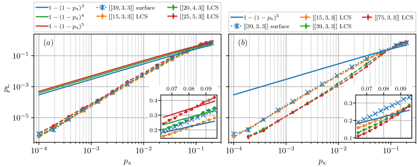
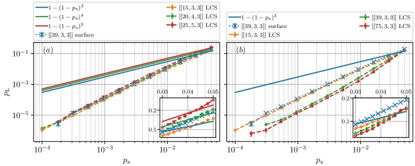
Figure 8: Logical error rates of small LCS codes, sampled over a bit-flip channel and decoded using the MLE decoder (Sec. IV.2.1). (a) Codes with $\ell=1$ and $L=2,3,4$, compared to error probabilities of $3,4$ and $5$ physical qubits (solid lines), respectively. The smallest distance $3$ code has the lowest logical error rate. The curves cross the physical qubit curves at the pseudo-threshold $p^{\star}_{\mathrm{th}}\approx 8.6\%$. (b) Codes with $\ell=1,2,3$ and $L=3$, compared to error probabilities of $3$ physical qubits and $3$ copies of $[[13,1,3]]$ surface codes. Interconnected codes can achieve the same logical error rate as surface codes using less physical qubits (here $15$ vs. $39$). Using more physical qubits increasing the redundancy gives an improvement of almost one order of magnitude for low physical error probabilities. The pseudo-threshold is also increased from $p^{\star}_{\mathrm{th}}(3\cdot[[13,1,3]]-\text{S})\approx 6\%$ to $p^{\star}_{\mathrm{th}}([[39,3,3]]-\text{LCS})\approx 8.6\%$. In this plot and all following, statistical error bars corresponding to one standard deviation in the Monte Carlo sampling are drawn (occasionally smaller than markers).

Figure 9: Logical error rates of small LCS codes, sampled over a bit-flip channel with $d$ noisy syndrome measurements and decoded using the MLE decoder (Sec. IV.2.1). (a) Codes with $\ell=1$ and $L=2,3,4$, compared to error probabilities of $3,4$ and $5$ physical qubits, respectively. The smallest distance $3$ code has the lowest logical error rate. The curves cross the physical qubit curves at the pseudo-threshold $p^{\star}_{\mathrm{th}}\approx 4.2\%$. (b) Codes with $\ell=1,2,3$ and $L=3$, compared to error probabilities of $3$ physical qubits and $3$ copies of $[[13,1,3]]$ surface codes. Interconnected codes can achieve the same logical error rate as surface codes using less physical qubits (here $15$ vs. $39$). Using more physical qubits increasing the redundancy gives an improvement of almost one order of magnitude for low physical error probabilities. The pseudo-threshold is also increased from $p^{\star}_{\mathrm{th}}(3\cdot[[13,1,3]]-\text{S})\approx 3\%$ to $p^{\star}_{\mathrm{th}}([[39,3,3]]-\text{LCS})\approx 4.6\%$.

IV.3.4 Code families and their thresholds

Beyond pseudo-thresholds of specific codes, the asymptotic threshold of families of code is of interest, in particular in order to compare the performance of different code families.

It is important to note that the existence of a threshold has been proven for concatenated codes [65, 1], codes with an asymptotically constant encoding rate [66, 11] and topological codes with rate vanishing $r\propto n^{-1}$ [8]. For general QLDPC codes, the existence of and lower bounds on a threshold were proven subsequently [67]. The threshold of a code family under a specific noise model and decoder is typically determined by Monte Carlo sampling and plotting the logical error rate versus the physical error rate for representatives of the code family with growing number of physical qubits and code distance. Heuristically, a crossing of these curves at a point $p=p^{\star}$ indicates the existence of a threshold at $p^{\star}$. This is supported by arguments from statistical mechanics mappings of error correcting codes and is particularly successful for topological codes with well defined scaling properties [68, 69, 70]. Hence for independent copies of surface codes we can expect the same asymptotic threshold as the copies fail independently. Results for $k=1$ logical qubits that are rescaled according to Eq. 46 however have finite size crossing points of the curves that deviate from the asymptotic threshold. For general QLDPC codes, the statistical mechanical picture is more intricate and far less well understood and part of ongoing research [71, 72]. Nevertheless, crossing points of such curves give an estimate on the value of the threshold.

From all available code parameters when sweeping $\ell,L$ (Fig. 4) we can define code families which are suitable for comparative simulations of error correcting properties. In the following, we will define three relevant scenarios and report the numerical findings. Note that all data for surface codes is obtained with the same BP+OSD decoder used for LCS codes for direct comparison.

1. Same parameter LCS code: Enforcing the parameters $[[n,k,d]]$ of surface (subindex $s$) and LCS codes to be the same corresponds to taking $L$ copies of distance $L$ surface codes and interconnecting them. Hence, this scenario explores the influence of the higher stabilizer weights with 2D non-local connectivity. This is achieved by setting $\ell_{s}=\ell=L-1=L_{s}-1$, such that the parameters are

   $$[[n,k,d]]_{\text{lcs}}=[[n,k,d]]_{\text{s}}=[[(2L^{2}-2L+1)L,L,L]].$$ (62)

   These families are marked dark green in Fig. 4.

   Under code capacity noise, Fig. 11 $(a)$ shows the logical error rate of any logical qubit compared to the physical bit-flip probability. With growing $n,d$, the logical error rate is increasingly suppressed. Compared to copies of surface codes, the interconnected LCS codes show a logical error rate that is up to 2 orders of magnitude lower at physical error rates on the order of $10^{-2}$. We observe a crossing of curves with at $p^{\star}\approx 6.5-7\%$ indicating a threshold of $\approx 6.7\pm 0.3\%$, slightly lower than the crossing point for surface codes at $p^{\star}\approx 7.5\pm 0.3\%$. All indicated uncertainties on threshold values are readoff errors estimating how well we can resolve the respective crossing point.

   Results using the phenomenological noise model decoded with the adapted BP+OSD decoder are shown in Fig. 11 $(a)$. The results qualitatively show similar trends as for the previous code capacity case. To pick out a striking example, at a physical error rate of $10^{-2}$, the logical error rate of the $[[595,7,7]]$ LCS code is 2 orders of magnitude lower compared to the surface code. The estimated threshold value we report for this code family under phenomenological noise is $\approx 2.9\pm 0.1\%$ which within resolution coincides with the surface code family threshold $\approx 2.9\pm 0.1\%$.

2. Highest rate LCS code for fixed dimension and distance. We can see in Fig. 4 that for the same $k,d$, we can tune the parameter $\ell$ for the LCS codes to a higher and lower rate. The highest rate is achieved by setting $\ell=\frac{L-1}{2}$. These LCS codes are depicted in Fig. 4 by purple rectangles. This family includes representatives of codes with the smallest number of physical qubits while having distances $d\geq 3$. We compare this family to surface codes with the same number of logical qubits $k$ and distance $d$, which gives

   $$[[n,k,d]]_{\text{lcs}} =[[\frac{1}{2}(L^{2}+1)L,L,L]],$$ (63)

   $$[[n,k,d]]_{\text{s}} =[[(2L^{2}-2L+1)L,L,L]].$$ (64)

   This implies a saving of a factor 4 in qubit number for the same rate and distance for sufficiently large $L$.

   The simulation results under code capacity noise are shown in Fig. 11 $(b)$. Also in this scenario, we find a lower logical error rate for the LCS family, which can be attributed to the smaller number of physical qubits. However the gain is smaller compared to lower rate codes which can be explained with the higher degeneracy of lower rate codes. We also observe a crossing of curves at a slightly higher $p^{\star}\approx 7.7\pm 0.2\%$ indicating a threshold in that vicinity.

   Under phenomenological noise (Fig. 11 $(b)$) for the given scenario the crossing indicates a threshold estimate of $\approx 3.2\pm 0.1\%$ compared to $\approx 2.9\pm 0.1\%$ for the corresponding surface codes. The slight deviation in favor of the LCS family should be interpreted cautiously.

3. Largest distance LCS code for fixed physical and logical qubit number. This compares codes with parameters

   $$[[n,k,d]]_{\text{lcs}} =[[\frac{1}{2}(L^{2}+1)L,L,L]],$$ (65)

   $$[[n,k,d]]_{\text{s}} =[[\frac{1}{2}(L^{2}+1)L,L,\frac{L+1}{2}]].$$ (66)

   This implies a factor of 2 improvement in distance for same qubit number and rate for sufficiently large $L$.

   The logical error rates for this scenario under code capacity noise are shown in Fig. 11 $(c)$ and under phenomenological noise in Fig. 11 $(c)$. Here, we observe the largest gain among the three scenarios, i.e. when fixing the number of physical qubits and the desired code rate, choosing LCS codes over surface codes leads to the largest improvement in logical error rate. This can likely be attributed to the fact that the corresponding surface codes have a smaller distance $d_{\mathrm{s}}=\frac{d_{\mathrm{lcs}}+1}{2}$. Compared to the example in the ”same parameter scenario”, here we observe an improvement of 2 orders of magnitude at physical error rate $p=10^{-2}$ already for the even smaller $[[369,9,9]]$ LCS code compared to the corresponding nine copies of distance five surface codes with parameters $[[369,9,5]]$. Note that the threshold values for this scenario are the same as in the previous scenario.

Overall, these results indicate that LCS codes systematically offer improved performance in terms of logical error rate compared to standard surface codes under both code capacity and phenomenological noise.

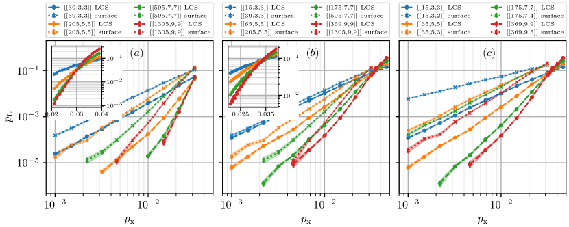
Figure 10: Logical error rate of LCS codes under code-capacity bit-flip noise using the BP+OSD decoder compared to surface codes. We compare three different parameter scaling choices, for all of which we observe a reduction of logical error rate with growing $n,d$. (a) Codes are chosen such that LCS and surface codes have the same parameters $[[n,k,d]]$. The logical error rate for the interconnected codes is up to 2 orders of magnitude lower than for the surface codes at a physical error rate in the order of $10^{-2}$. We also observe a crossing of the curves indicating the existence of a threshold at $\approx 6.7\pm 0.3\%$ . (b) LCS codes are chosen such that they have the lowest qubit number $n$ for same $k,d$. As explained in the text, there is still a reduction in logical error rate compared to disjoint surface codes, however this is less pronounced than in the setting discussed previously. The crossing of the curves indicates a slightly higher threshold at $\approx 7.7\pm 0.2\%$. (c) Codes chosen such that for the same $n,k$, LCS codes have highest available distance. Here we observe the largest reduction in logical error rate. Note that this is consistent with the expectation that the distance is closely related to the number of correctable errors.

Figure 11: Logical error rate of LCS codes under phenomenological bit-flip noise using the BP+OSD decoder compared to surface codes. We report the logical error rate per round and compare three different parameter scaling choices, for all of which we observe a reduction of logical error rate with growing $n,d$. (a) Codes are chosen such that LCS and surface codes have the same parameters $[[n,k,d]]$. The logical error rate for the interconnected codes is up to 2 orders of magnitude lower than for the surface codes at a physical error rate in the order of $10^{-2}$. We also observe a crossing of the curves in the vicinity of $\approx 2.9\pm 0.1\%$ indicating the existence of a threshold. (b) LCS codes are chosen such that they have the lowest qubit number for same $k,d$. As explained in the text, there is still a reduction in logical error rate compared to disjoint surface codes, however not as large. The crossing of the curves indicates a slightly higher threshold at $\approx 3.2\pm 0.1\%$. (c) Codes chosen such that for the same $n,k$, LCS codes have highest available distance. Again, note that this is consistent with the expectation that the distance is closely related to the number of correctable errors.

V Towards logical gates in LCS codes

Implementing logical gates in QLDPC codes is a hard challenge, in particular if the implementation is to be fault-tolerant. In the following, we show a particular set of fault-tolerant gates for LCS codes when fixing $\ell=1$. These have an almost planar geometrical representation and useful symmetries. Three representatives ($L=2,3,4$) are shown in Fig. 12. They correspond to codes with parameters $[[n,k,d]]=[[10,1,2]],[[15,3,3]]$ and $[[20,4,3]]$ respectively. They have a symmetry also called $ZX$-duality that exchanges $X$- and $Z$- stabilizers by simple swaps but keeps logical operators invariant. This symmetry is easily seen in the parity check matrices for $\ell=1$,

Swapping the second and third block, i.e. applying the column permutation

brings $\tilde{H}_{X}\to\tilde{H}_{Z}$ and vice versa. Logical operators of these codes are given by

and therefore left invariant under $\tau$.

This duality enables several fold-transversal gates, in particular a fold-transversal Hadamard that implements a global logical Hadamard [44],

$$\overline{H}=\bigotimes_{i<\tau(i)}\operatorname*{SWAP}(i,\tau(i))\bigotimes_{i=1}^{n}H_{i}=\bigotimes_{i=1}^{k}\overline{H}_{i}$$ (67)

and a fold-transversal Phase gate

$$\overline{S}=\bigotimes_{i\in A}S_{i}\bigotimes_{i\in B}S^{\dagger}_{i}\bigotimes_{\begin{subarray}{c}i=1,\dots,n\\ i<\tau(i)\end{subarray}}\mathrm{CZ}_{i,\tau(i)}.$$ (68)

In the latter, $A$ and $B$ are partitions of the qubits not involved in $\tau$ such that every $X$-stabilizer has half support on $A$ and $B$ respectively. These are also indicated by empty and filled circles in Fig. 12 for the $[[15,3,3]]$-LCS code. The $\mathrm{CZ}$s ensure that the stabilizer group is invariant by mapping $S_{X}\to S_{X}S_{Z}$ since for single-qubit Paulis $\mathrm{CZ}_{ij}X_{i}\mathrm{CZ}_{ij}=X_{i}Z_{j}$. The phase gate acts as $S_{i}X_{i}S_{i}^{\dagger}=iX_{i}Z_{i}$ and $S_{i}^{\dagger}X_{i}S_{i}=-iX_{i}Z_{i}$, such that the partitioning guarantees unwanted phase factors to cancel out. We can verify that the fold-transversal Phase gate implements a global logical Phase gate $\overline{S}=\otimes_{i=1}^{k}\overline{S}_{i}$.

These gates can be supplemented by the transversal $\overline{\mathrm{CNOT}}$ [73] to generate the full Clifford group on the set of logical qubits of copies of these $d=3$ LCS codes. A universal set of fault-tolerant gates operating on single logical qubits is an open challenge. Approaches towards that goal may be based on (generalized) lattice surgery and gate teleportation [74, 45, 46], pieceable fault-tolerance [75] or code switching [76, 77]. Generalizing existing approaches for HGP codes [48, 40] to LP codes are another promising avenue.

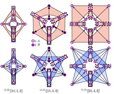
Figure 12: First three members of $\ell=1$ LCS codes. $X$- (top) and $Z$-stabilizers (bottom). Logical operators shown in squares with different line styles for $X$ and $Z$ logical operators respectively. Note that they can be chosen to have same support. Swapping pairs of qubits on a diagonal as shown exemplarily for the $k=2$ and $k=4$ codes swaps $X$ and $Z$ stabilizers while leaving logical operators invariant. For $k=3$ (center), the partitions $A$ and $B$, as well the the $\mathrm{CZ}$ operations of the fold-transversal Phase gate are indicated (cf. Eq. 68).

VI Conclusion

We have introduced lift-connected surface (LCS) codes as a new family of QLDPC codes based on the lifted product construction. We have shown how they can be viewed as interconnected copies of surface codes and how this additional connectivity leads to favorable parameters compared to disjoint copies of surface codes. We adapted a BP+OSD decoder to the phenomenological noise setting and performed benchmarking of LCS codes for code-capacity and phenomenological noise. We observed that, while asymptotic thresholds are comparable to those of standard surface codes, the pseudo-thresholds can be significantly higher and logical error rates much lower. These advantages in particular also hold for small codes with qubit number below 100.

Implementing the stabilizer measurements of the codes in general involves coupling the data qubits to ancilla qubits by gates. These introduce another source of noise, that is captured by a circuit level noise model. Investigating the performance of LCS codes under circuit level noise will hinge on the construction of fault-tolerant circuits. For hypergraph product codes, constructions of distance-preserving circuits have been recently introduced [23, 33, 78], a generalization to lifted product codes would be highly desirable. Other modern fault-tolerant circuit constructions such as using flag-qubits [79] should facilitate resource efficient and fault-tolerant stabilizer readout protocols. The circuit construction also depends on assumptions on available gates and connectivity. Given that LCS codes are embeddable in three dimensions with local connectivity, this makes them highly attractive for near-term platforms and particularly suited for the emerging platforms of static 3D optical lattices or reconfigurable 2D arrays of Rydberg atoms [53, 7].

Appendix A Block structure of parity check matrices and distance of LCS codes

The block structure of the parity check matrices of the LCS codes is shown in Fig. 13, exemplarily for $(\ell,L)=(2,4)$ ($[[52,4,4]]$). The parity check matrices inherit the block structure from the HGP, which can for example be seen in the block-diagonal structure of $H_{X}$. In total, the binary parity check matrices consist of $\ell(\ell+1)\times(2\ell^{2}+2\ell+1)$ blocks of size $L\times L$. Note that both $H_{X}$ and $H_{Z}$ are in row echelon form.

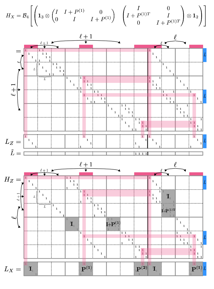
Figure 13: Block structure of the parity check matrices of $X$- (Top) and $Z$-stabilizers (bottom), exemplarily for $(\ell,L)=(2,4)$. Note that the block structure is inherited from the HGP product. The red rectangles on top of the matrices indicate the positions of the diagonal logicals in the regular HGP surface code. Also shown are matrices $L_{Z}$ and $L_{X}$ that are the binary representation of logical $Z$- and $X$-operators. They can be found as described in the text and have weight $2\ell+1$. For the first logical operators, the overlap with the stabilizers of the respective other Pauli type is drawn in a red shade, visualizing the commutation. Additionally, we show the operator $\tilde{L}$ of weight $L$ which can be constructed from products of all logical operators and some stabilizers as described in the text and shown with blue rectangles on the right side of the matrices.

This particular form of the parity check matrices allows us to construct set of logical operators. If we have a set of $k$ independent generators of logical operators and find their minimal weight, we can find the minimum distance of the code. By carefully inspecting the parity check matrices, we explicitly construct $L=k$ logical operators of weight $2\ell+1$. To that end, it is useful to first realize that, in regular surface codes, we can choose representatives of logical $X$- and $Z$- operators to have the same support by putting them on the diagonal. Indexing each column of the left with tuples $(i,j)\in\{0,1,\dots,\ell\}^{2}$ and for the right block with tuples $(i,j)\in\{0,1,\dots,\ell-1\}^{2}$, these diagonal qubits can be identified with columns $(0,0),(1,1),(2,2),\dots,(\ell,\ell)$ in the left part of the parity check matrices and columns $(0,0),(1,1),(2,2),\dots,(\ell-1,\ell-1)$ of the right part. These positions are also indicated by red boxes at the top of the parity check matrices in Fig. 13. The lift requires to select circulants at these positions, such that the resulting operators are also logical operators. It turns out that choosing logicals (before lifting $L$ times) of the form

$$\big{(}\underbrace{\underbrace{\matrixquantity{1&0&\cdots&0}}_{\ell+1}|\matrixquantity{0&P^{(1)}&0&\cdots&0}|\matrixquantity{0&0&P^{(2)}&0&\cdots&0}|\cdots|\matrixquantity{0&\cdots&0&P^{(\ell)}}}_{\ell+1}||\underbrace{\underbrace{\matrixquantity{1&0&\cdots&0}}_{\ell}|\matrixquantity{0&P^{(1)}&0&\cdots&0}|\cdots|\matrixquantity{0&\cdots&0&P^{(\ell-1})}}_{\ell}\big{)}$$ (69)

ensures that every stabilizer has even overlap with the logicals. Note that in column $(i,i)$ (of both left and right part), the circulant $P^{(i)}$ is placed. These are also shown in Fig. 13 for the $[[52,4,4]]$ code. As binary representations of logical $X$- and $Z$-operators, these are $L$ pairs of disjoint operators since they only consist of circulants with one term, i.e. cyclic permutation matrices. With the respective partner ($L_{X}^{i},L_{Z}^{i}$), the anti-commutation is guaranteed by the odd weight $2\ell+1$. Finally, these operators cannot have their weight reduced by adding stabilizers, which can also be verified using the block-structure of the parity check matrices. Every attempt to reduce the weight necessarily introduces new qubit connectivity.

However, taking the product of all these $L$ operators results in an operator with ones in all the columns specified above. Multiplying stabilizers of rows $(0,0),(1,1),\dots,(\ell-1,\ell-1)$ will give an operator of (potentially lower) weight $L$.

We therefore found a set of $L$ independent operators, each of minimum weight $2\ell+1$. Their sum has minimum weight $L$ and all other combinations of stabilizer and logical operator have weight $\geq 2\ell+1$ . We have therefore further evidence that the minimum distance of the code is

$$d=\min(2\ell+1,L).$$ (70)

Appendix B Parameters for BP+OSD decoding

The BP+OSD decoder used in Sec. IV has a range of parameters that influence the decoding performance. For a comprehensive overview, refer to the source code [62]. Important parameters used in these simulations are shown in Tab. 4. We observed that the (standard, but more complex) product sum method of BP (also described in the text) performs better than the lower complexity minimum sum method also provided by the package. The maximum number of BP iterations and the OSD order are also set heuristically based on observations in the decoding. For the $[[369,9,9]]$-LCS code, logical error rates for code capacity noise and different numbers of BP iterations are shown in Fig. 14. For different codes, we show the logical error rate for different numbers of BP iterations at a fixed physical error rate $p=0.0129$ in Fig. 15. Heuristically, we find good performance if we set the maximum number of BP iterations to $\frac{d-1}{2}$. We attribute this to the observation that if BP is not successful, a large number of iterations will lead to an ”overfitting” and move us away from configurations, where the OSD post-processing step guesses the logical error correctly. Increasing the OSD order gives improved results at the cost of run time, which is why we limit the order to $60$.

Table 4: Parameters used for BP+OSD decoding. Here, $[[n,k,d]]$ refer to the code parameters

Parameter	Value
BP method	product sum
maximum BP iterations	$\frac{d-1}{2}$
osd order	$\min(d^{2},60)$

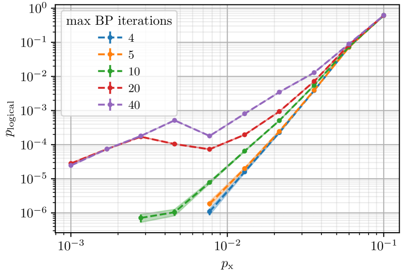
Figure 14: Logical error rate for the $[[369,9,9]]$-code using BP+OSD with different maximum BP iterations. Using only $4$ iterations gives the lowest logical error rate.

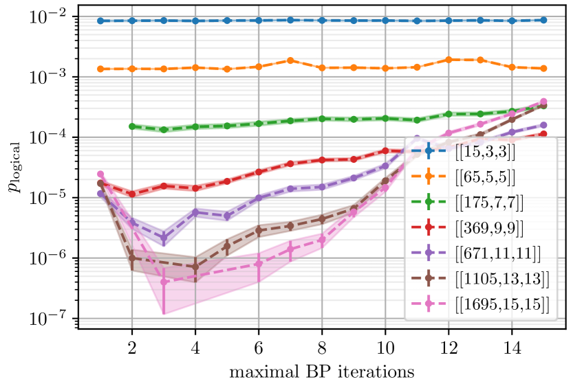
Figure 15: Logical error rates for the LCS-codes of family 2 (see main text Sec. IV.3.4) using BP+OSD with different maximum BP iterations. In particular for larger codes, the logical error rate is highly dependent on the maximum number of BP iterations before OSD post-processing.

Appendix C Validity of BP+OSD decoding

To verify the validity of BP+OSD decoding, we compare the most-likely error decoder to the BP+OSD decoder. As can be seen in Fig. 16, they perform very similarly for small qubit numbers, but for many qubits and low error rate, the decoding performance of BP+OSD decreases.

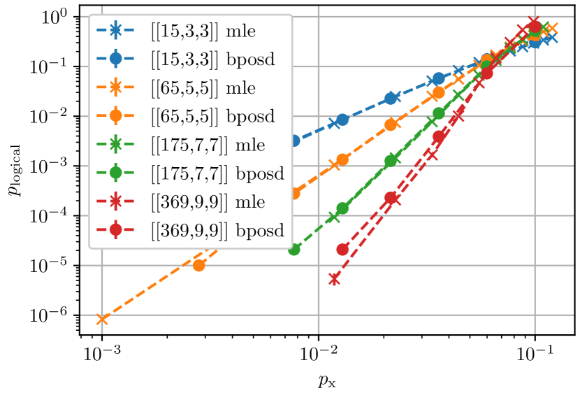
Figure 16: Logical error rate for LCS codes (family 2, see main text Sec. IV.3.4) using MLE and BP+OSD. In particular for low qubit numbers, BP+OSD comes close to MLE decoding.

Appendix D Sampling Methods

The implementation details of the sampling for code capacity noise and phenomenological noise are shown in Alg. 1 and Alg. 2 respectively.

Input: Quantum Channel $\mathcal{E}$, physical error probabilities $\mathbf{p}_{\text{phys}}=(p_{x},p_{y},p_{z})$, number of samples $n$, Quantum Code $\mathcal{Q}$

Output: Number of successful runs $n_{\text{success}}$

$n_{\text{success}}=0$

for $i=0$, $i<n$, $i=i+1$ do

       $E=\mathcal{E}(0,\mathbf{p})$

       $\mathbf{s}=\sigma(E)$

       $E^{\star}=\mathrm{Dec}(\mathbf{s},\mathbf{p},\dots)$

       if $\sigma(EE^{\star})=0\;\&\;\langle EE^{\star},L\rangle=0\quad\forall L\in\mathcal{L}(\mathcal{Q})$ then

            $n_{\text{success}}=n_{\text{success}}+1$

       end if

      

end for

return $n_{\text{success}}$

Algorithm 1 Code capacity sampling of quantum codes

Input: Quantum Channel $\mathcal{E}$, physical qubit error probabilities $\mathbf{p}_{\text{phys}}=(p_{x},p_{y},p_{z})$, Classical Channel $\mathcal{B}$, physical syndrome error probability $q$, number of samples $n$, Quantum Code $\mathcal{Q}$

Output: Number of successful runs $n_{\text{success}}$

$n_{\text{success}}=0$

for $i=0$, $i<n$, $i=i+1$ do

       $E=0$

       $\mathbf{s}=(0)^{((t+1)\times n_{c})}$

       for $t=0$, $t,d(\mathcal{Q})$, $t=t+1$ do

             $E=\mathcal{E}(E,\mathbf{p})$

             $\mathbf{s}_{t+1}=\mathcal{B}(\sigma(E))$

            

       end for

      $E^{\star}=\mathrm{Dec_{1}}(\mathbf{s},\mathbf{p},q,\dots)$

       $\mathbf{s}^{\star}=\sigma(EE^{\star})$

       $E^{\star\star}=\mathrm{Dec_{2}}(\mathbf{s}^{\star},\mathbf{p},\dots)$

       if $\sigma(EE^{\star}E^{\star\star})=0\;\&\;\langle EE^{\star}E^{\star\star},L\rangle=0\quad\forall L\in\mathcal{L}(\mathcal{Q})$ then

            $n_{\text{success}}=n_{\text{success}}+1$

       end if

      

end for

return $n_{\text{success}}$

Algorithm 2 Phenomenological noise sampling of quantum codes

References

- Knill et al. [1998] E. Knill, R. Laflamme, and W. H. Zurek, Resilient quantum computation: error models and thresholds, Proceedings of the Royal Society of London. Series A: Mathematical, Physical and Engineering Sciences 454, 365 (1998).
- Ryan-Anderson et al. [2021] C. Ryan-Anderson, J. Bohnet, K. Lee, D. Gresh, A. Hankin, J. Gaebler, D. Francois, A. Chernoguzov, D. Lucchetti, N. Brown, et al., Realization of real-time fault-tolerant quantum error correction, Physical Review X 11, 041058 (2021).
- Postler et al. [2022] L. Postler, S. Heußen, I. Pogorelov, M. Rispler, T. Feldker, M. Meth, C. D. Marciniak, R. Stricker, M. Ringbauer, R. Blatt, P. Schindler, M. Müller, and T. Monz, Demonstration of fault-tolerant universal quantum gate operations, Nature 605, 675 (2022).
- Hilder et al. [2022] J. Hilder, D. Pijn, O. Onishchenko, A. Stahl, M. Orth, B. Lekitsch, A. Rodriguez-Blanco, M. Müller, F. Schmidt-Kaler, and U. Poschinger, Fault-tolerant parity readout on a shuttling-based trapped-ion quantum computer, Physical Review X 12, 011032 (2022).
- Krinner et al. [2022] S. Krinner, N. Lacroix, A. Remm, A. D. Paolo, E. Genois, C. Leroux, C. Hellings, S. Lazar, F. Swiadek, J. Herrmann, G. J. Norris, C. K. Andersen, M. Müller, A. Blais, C. Eichler, and A. Wallraff, Realizing repeated quantum error correction in a distance-three surface code, Nature 605, 669 (2022).
- Google Quantum AI [2023] Google Quantum AI, Suppressing quantum errors by scaling a surface code logical qubit, Nature 614, 676 (2023).
- Bluvstein et al. [2023] D. Bluvstein, S. J. Evered, A. A. Geim, S. H. Li, H. Zhou, T. Manovitz, S. Ebadi, M. Cain, M. Kalinowski, D. Hangleiter, J. P. B. Ataides, N. Maskara, I. Cong, X. Gao, P. S. Rodriguez, T. Karolyshyn, G. Semeghini, M. J. Gullans, M. Greiner, V. Vuletic, and M. D. Lukin, Logical quantum processor based on reconfigurable atom arrays, arXiv 10.1038/s41586-023-06927-3 (2023), 2312.03982 .
- Kitaev [1997] A. Y. Kitaev, Quantum computations: algorithms and error correction, Russian Mathematical Surveys 52, 1191 (1997).
- Stephens [2014] A. M. Stephens, Fault-tolerant thresholds for quantum error correction with the surface code, Phys. Rev. A 89, 022321 (2014).
- Fowler et al. [2012a] A. G. Fowler, M. Mariantoni, J. M. Martinis, and A. N. Cleland, Surface codes: Towards practical large-scale quantum computation, Phys. Rev. A 86, 032324 (2012a).
- Gottesman [2013] D. Gottesman, Fault-tolerant quantum computation with constant overhead, arXiv preprint arXiv:1310.2984 10.48550/arXiv.1310.2984 (2013).
- MacKay et al. [2004] D. J. C. MacKay, G. Mitchison, and P. L. McFadden, Sparse-graph codes for quantum error correction, IEEE Trans. Inf. Theory 50, 2315 (2004).
- Breuckmann and Eberhardt [2021a] N. P. Breuckmann and J. N. Eberhardt, Quantum low-density parity-check codes, PRX Quantum 2, 040101 (2021a).
- Tillich and Zémor [2013] J.-P. Tillich and G. Zémor, Quantum ldpc codes with positive rate and minimum distance proportional to the square root of the blocklength, IEEE Transactions on Information Theory 60, 1193 (2013).
- Sipser and Spielman [1996] M. Sipser and D. A. Spielman, Expander codes, IEEE Trans. Inf. Theory 42, 1710 (1996).
- Breuckmann and Eberhardt [2021b] N. P. Breuckmann and J. N. Eberhardt, Balanced product quantum codes, IEEE Transactions on Information Theory 67, 6653 (2021b).
- Panteleev and Kalachev [2022a] P. Panteleev and G. Kalachev, Asymptotically good quantum and locally testable classical ldpc codes, in Proceedings of the 54th Annual ACM SIGACT Symposium on Theory of Computing (2022) pp. 375–388.
- Leverrier and Zémor [2022] A. Leverrier and G. Zémor, Quantum tanner codes, arXiv preprint arXiv:2202.13641 10.48550/arXiv.2202.13641 (2022).
- Dinur et al. [2023] I. Dinur, M.-H. Hsieh, T.-C. Lin, and T. Vidick, Good quantum ldpc codes with linear time decoders (Association for Computing Machinery, New York, NY, USA, 2023) p. 905–918.
- Bravyi and Terhal [2009] S. Bravyi and B. Terhal, A no-go theorem for a two-dimensional self-correcting quantum memory based on stabilizer codes, New Journal of Physics 11, 043029 (2009).
- Bravyi et al. [2010] S. Bravyi, D. Poulin, and B. Terhal, Tradeoffs for reliable quantum information storage in 2d systems, Phys. Rev. Lett. 104, 050503 (2010).
- Delfosse et al. [2021] N. Delfosse, M. E. Beverland, and M. A. Tremblay, Bounds on stabilizer measurement circuits and obstructions to local implementations of quantum ldpc codes, arXiv preprint arXiv:2109.14599 (2021).
- Tremblay et al. [2022] M. A. Tremblay, N. Delfosse, and M. E. Beverland, Constant-overhead quantum error correction with thin planar connectivity, Phys. Rev. Lett. 129, 050504 (2022).
- Bravyi et al. [2023] S. Bravyi, A. W. Cross, J. M. Gambetta, D. Maslov, P. Rall, and T. J. Yoder, High-threshold and low-overhead fault-tolerant quantum memory, arXiv 10.48550/arXiv.2308.07915 (2023), 2308.07915 .
- Strikis and Berent [2023] A. Strikis and L. Berent, Quantum low-density parity-check codes for modular architectures, PRX Quantum 4, 020321 (2023).
- Bruzewicz et al. [2019] C. D. Bruzewicz, J. Chiaverini, R. McConnell, and J. M. Sage, Trapped-ion quantum computing: Progress and challenges, Applied Physics Reviews 6, 021314 (2019).
- Kaushal et al. [2020] V. Kaushal, B. Lekitsch, A. Stahl, J. Hilder, D. Pijn, C. Schmiegelow, A. Bermudez, M. Müller, F. Schmidt-Kaler, and U. Poschinger, Shuttling-based trapped-ion quantum information processing, AVS Quantum Science 2, 014101 (2020).
- Saffman [2016] M. Saffman, Quantum computing with atomic qubits and Rydberg interactions: progress and challenges, J. Phys. B: At. Mol. Opt. Phys. 49, 202001 (2016).
- Moses et al. [2023] S. A. Moses et al., A race track trapped-ion quantum processor, arXiv preprint arXiv:2305.03828 (2023), arXiv:2305.03828 [quant-ph] .
- Bluvstein et al. [2022] D. Bluvstein, H. Levine, G. Semeghini, T. T. Wang, S. Ebadi, M. Kalinowski, A. Keesling, N. Maskara, H. Pichler, M. Greiner, et al., A quantum processor based on coherent transport of entangled atom arrays, Nature 604, 451 (2022).
- Wu et al. [2022] Y. Wu, S. Kolkowitz, S. Puri, and J. D. Thompson, Erasure conversion for fault-tolerant quantum computing in alkaline earth Rydberg atom arrays, Nat. Commun. 13, 1 (2022).
- Cong et al. [2022] I. Cong, H. Levine, A. Keesling, D. Bluvstein, S.-T. Wang, and M. D. Lukin, Hardware-efficient, fault-tolerant quantum computation with rydberg atoms, Physical Review X 12, 021049 (2022).
- Xu et al. [2023] Q. Xu, J. P. B. Ataides, C. A. Pattison, N. Raveendran, D. Bluvstein, J. Wurtz, B. Vasic, M. D. Lukin, L. Jiang, and H. Zhou, Constant-Overhead Fault-Tolerant Quantum Computation with Reconfigurable Atom Arrays, arXiv 10.48550/arXiv.2308.08648 (2023), 2308.08648 .
- Panteleev and Kalachev [2021] P. Panteleev and G. Kalachev, Degenerate Quantum LDPC Codes With Good Finite Length Performance, Quantum 5, 585 (2021), 1904.02703v3 .
- Roffe et al. [2020] J. Roffe, D. R. White, S. Burton, and E. Campbell, Decoding across the quantum low-density parity-check code landscape, Physical Review Research 2, 10.1103/physrevresearch.2.043423 (2020).
- Delfosse et al. [2022] N. Delfosse, V. Londe, and M. E. Beverland, Toward a Union-Find Decoder for Quantum LDPC Codes, IEEE Trans. Inf. Theory 68, 3187 (2022).
- Berent et al. [2023] L. Berent, L. Burgholzer, and R. Wille, Software Tools for Decoding Quantum Low-Density Parity-Check Codes, in ASPDAC ’23: Proceedings of the 28th Asia and South Pacific Design Automation Conference (Association for Computing Machinery, New York, NY, USA, 2023) pp. 709–714.
- Leverrier and Zémor [2023] A. Leverrier and G. Zémor, Efficient decoding up to a constant fraction of the code length for asymptotically good quantum codes, in Proceedings of the 2023 Annual ACM-SIAM Symposium on Discrete Algorithms (SODA) (Society for Industrial and Applied Mathematics, 2023) pp. 1216–1244.
- Gu et al. [2023] S. Gu, C. A. Pattison, and E. Tang, An efficient decoder for a linear distance quantum ldpc code, in Proceedings of the 55th Annual ACM Symposium on Theory of Computing, STOC 2023 (Association for Computing Machinery, New York, NY, USA, 2023) p. 919–932.
- Quintavalle et al. [2021] A. O. Quintavalle, M. Vasmer, J. Roffe, and E. T. Campbell, Single-shot error correction of three-dimensional homological product codes, PRX Quantum 2, 020340 (2021).
- Higgott and Breuckmann [2023] O. Higgott and N. P. Breuckmann, Improved Single-Shot Decoding of Higher-Dimensional Hypergraph-Product Codes, PRX Quantum 4, 020332 (2023).
- Eastin and Knill [2009] B. Eastin and E. Knill, Restrictions on transversal encoded quantum gate sets, Phys. Rev. Lett. 102, 110502 (2009).
- Jochym-O’Connor et al. [2018] T. Jochym-O’Connor, A. Kubica, and T. J. Yoder, Disjointness of stabilizer codes and limitations on fault-tolerant logical gates, Physical Review X 8, 021047 (2018).
- Breuckmann and Burton [2022] N. P. Breuckmann and S. Burton, Fold-transversal clifford gates for quantum codes, arXiv preprint arXiv:2202.06647 (2022).
- Brun et al. [2015] T. A. Brun, Y.-C. Zheng, K.-C. Hsu, J. Job, and C.-Y. Lai, Teleportation-based fault-tolerant quantum computation in multi-qubit large block codes, arXiv preprint arXiv:1504.03913 10.48550/arXiv.1504.03913 (2015).
- Cohen et al. [2022] L. Z. Cohen, I. H. Kim, S. D. Bartlett, and B. J. Brown, Low-overhead fault-tolerant quantum computing using long-range connectivity, Sci. Adv. 8, 10.1126/sciadv.abn1717 (2022).
- Jochym-O’Connor [2019] T. Jochym-O’Connor, Fault-tolerant gates via homological product codes, Quantum 3, 120 (2019), 1807.09783v2 .
- Krishna and Poulin [2021] A. Krishna and D. Poulin, Fault-tolerant gates on hypergraph product codes, Phys. Rev. X 11, 011023 (2021).
- Quintavalle et al. [2023] A. O. Quintavalle, P. Webster, and M. Vasmer, Partitioning qubits in hypergraph product codes to implement logical gates, Quantum 7, 1153 (2023).
- Panteleev and Kalachev [2022b] P. Panteleev and G. Kalachev, Quantum ldpc codes with almost linear minimum distance, IEEE Transactions on Information Theory 68, 213 (2022b).
- Tanner [1981] R. Tanner, A recursive approach to low complexity codes, IEEE Transactions on Information Theory 27, 533 (1981).
- Pryadko et al. [2022] L. P. Pryadko, V. A. Shabashov, and V. K. Kozin, Qdistrnd: A gap package for computing the distance of quantum error-correcting codes, Journal of Open Source Software 7, 4120 (2022).
- Barredo et al. [2018] D. Barredo, V. Lienhard, S. de Léséleuc, T. Lahaye, and A. Browaeys, Synthetic three-dimensional atomic structures assembled atom by atom, Nature 561, 79 (2018).
- Fowler et al. [2012b] A. G. Fowler, A. C. Whiteside, and L. C. L. Hollenberg, Towards Practical Classical Processing for the Surface Code, Phys. Rev. Lett. 108, 180501 (2012b).
- Poulin and Chung [2008] D. Poulin and Y. Chung, On the iterative decoding of sparse quantum codes, arXiv 10.48550/arXiv.0801.1241 (2008), 0801.1241 .
- Landahl et al. [2011] A. J. Landahl, J. T. Anderson, and P. R. Rice, Fault-tolerant quantum computing with color codes, arXiv preprint arXiv:1108.5738 (2011).
- Jensen et al. [2017] K. Jensen, J. G.r. Cardoso, and N. Sonnenschein, Optlang: An algebraic modeling language for mathematical optimization, Journal of Open Source Software 2, 139 (2017).
- Makhorin [2011] A. Makhorin, Glpk (gnu linear programming kit) (2011).
- Gallager [1962] R. Gallager, Low-density parity-check codes, IRE Trans. Inf. Theory 8, 21 (1962).
- MacKay and Neal [1997] D. J. MacKay and R. M. Neal, Near shannon limit performance of low density parity check codes, Electronics letters 33, 457 (1997).
- Roffe [2019] J. Roffe, Quantum error correction: an introductory guide, Contemporary Physics 60, 226 (2019).
- Roffe [2022a] J. Roffe, BP+OSD: A decoder for quantum LDPC codes (2022a).
- Roffe [2022b] J. Roffe, LDPC: Python tools for low density parity check codes (2022b).
- Preskill [1997] J. Preskill, Fault-tolerant quantum computation, arXiv 10.48550/arXiv.quant-ph/9712048 (1997), quant-ph/9712048 .
- Aharonov and Ben-Or [2008] D. Aharonov and M. Ben-Or, Fault-tolerant quantum computation with constant error rate, SIAM Journal on Computing 38, 1207 (2008), https://doi.org/10.1137/S0097539799359385 .
- Kovalev and Pryadko [2013] A. A. Kovalev and L. P. Pryadko, Fault tolerance of quantum low-density parity check codes with sublinear distance scaling, Phys. Rev. A 87, 020304 (2013).
- Dumer et al. [2015] I. Dumer, A. A. Kovalev, and L. P. Pryadko, Thresholds for correcting errors, erasures, and faulty syndrome measurements in degenerate quantum codes, Phys. Rev. Lett. 115, 050502 (2015).
- Dennis et al. [2002] E. Dennis, A. Kitaev, A. Landahl, and J. Preskill, Topological quantum memory, J. Math. Phys. 43, 4452 (2002).
- Wang et al. [2003] C. Wang, J. Harrington, and J. Preskill, Confinement-Higgs transition in a disordered gauge theory and the accuracy threshold for quantum memory, Ann. Phys. 303, 31 (2003).
- Ohno et al. [2004] T. Ohno, G. Arakawa, I. Ichinose, and T. Matsui, Phase structure of the random-plaquette Z2 gauge model: accuracy threshold for a toric quantum memory, Nucl. Phys. B 697, 462 (2004).
- Kovalev et al. [2018] A. A. Kovalev, S. Prabhakar, I. Dumer, and L. P. Pryadko, Numerical and analytical bounds on threshold error rates for hypergraph-product codes, Phys. Rev. A 97, 062320 (2018).
- Rakovszky and Khemani [2023] T. Rakovszky and V. Khemani, The Physics of (good) LDPC Codes I. Gauging and dualities, arXiv 10.48550/arXiv.2310.16032 (2023), 2310.16032 .
- Shor [1996] P. W. Shor, Fault-tolerant quantum computation, arXiv 10.48550/arXiv.quant-ph/9605011 (1996), quant-ph/9605011 .
- Horsman et al. [2012] C. Horsman, A. G. Fowler, S. Devitt, and R. Van Meter, Surface code quantum computing by lattice surgery, New Journal of Physics 14, 123011 (2012).
- Yoder et al. [2016] T. J. Yoder, R. Takagi, and I. L. Chuang, Universal fault-tolerant gates on concatenated stabilizer codes, Physical Review X 6, 031039 (2016).
- Beverland et al. [2021] M. E. Beverland, A. Kubica, and K. M. Svore, Cost of universality: A comparative study of the overhead of state distillation and code switching with color codes, PRX Quantum 2, 020341 (2021).
- Butt et al. [2023] F. Butt, S. Heußen, M. Rispler, and M. Müller, Fault-Tolerant Code Switching Protocols for Near-Term Quantum Processors, arXiv 10.48550/arXiv.2306.17686 (2023), 2306.17686 .
- Manes and Claes [2023] A. G. Manes and J. Claes, Distance-preserving stabilizer measurements in hypergraph product codes, arXiv 10.48550/arXiv.2308.15520 (2023), 2308.15520 .
- Chamberland and Beverland [2018] C. Chamberland and M. E. Beverland, Flag fault-tolerant error correction with arbitrary distance codes, Quantum 2, 53 (2018).