Nonlinear functional regression by functional deep neural network with kernel embedding

Abstract

With the rapid development of deep learning in various fields of science and technology, such as speech recognition, image classification, and natural language processing, recently it is also widely applied in the functional data analysis (FDA) with some empirical success. However, due to the infinite dimensional input, we need a powerful dimension reduction method for functional learning tasks, especially for the nonlinear functional regression. In this paper, based on the idea of smooth kernel integral transformation, we propose a functional deep neural network with an efficient and fully-data-dependent dimension reduction method. The architecture of our functional net consists of a kernel embedding step: an integral transformation with a data-dependent smooth kernel; a projection step: a dimension reduction by projection with eigenfunction basis based on the embedding kernel; and finally an expressive deep ReLU neural network for the prediction. The utilization of smooth kernel embedding enables our functional net to be discretization invariant, efficient, and robust to noisy observations, capable of utilizing information in both input functions and responses data, and have a low requirement on the number of discrete points for an unimpaired generalization performance. We conduct theoretical analysis including approximation error and generalization error analysis, and numerical simulations to verify these advantages of our functional net.

Keywords: Deep learning theory, functional deep neural network, kernel smoothing, nonlinear functional, approximation rates, learning rates

1 Introduction

Functional data analysis (FDA) is a rising subject in recent scientific studies and daily life, which analyzes data with information about curves, surfaces, or anything else over a continuum, such as time, spatial location, and wavelength which are commonly considered in physical background, and each sample element of functional data is a random function defined on this continuum [38, 19]. In practice, our goal is to utilize these functional data to learn the relationship between the input function and the response, which can be either scalar or functional. On the other hand, deep learning has shown its great empirical success on various datasets such as audio, image, text and graph, due to its great power of automatically feature extraction based on data, and its flexibility on the architecture design for varieties of data formats. Therefore, it is a straightforward idea to consider applications of deep learning in FDA, and recently there are many researches concerning this approach. For example, for solving parametric partial differential equations (PDEs), [22, 27] aim at learning the map between the parametric function space and the solution space by the operator neural networks. There are also many attempts on image processing tasks with neural networks, such as phase retrieval [15], image super-resolution [35], image inpainting [36], and image denoising [52].

Along with the thirty decades development of the theoretical analysis of deep neural networks, recent works have quantitatively demonstrated the comparable approximation power of commonly used deep ReLU neural networks, which is as good as traditional deep neural networks with infinitely differentiable activation functions such as sigmoid and tanh activation functions [51, 57, 50, 59, 29], having such a strong expressivity together with its computational efficiency in the optimization stage partially explain the great empirical success of deep ReLU neural networks. Based on these approximation results, generalization analysis for the empirical risk minimization (ERM) algorithm with deep ReLU neural networks are also well developed [11, 44, 28]. However, such theoretical understanding on the deep learning approaches for functional data is still lacking, although there are some attempts in the literature [9, 30, 23, 7, 24, 10] for different architectures of operator (functional) neural networks such as Fourier neural operators, DeepONets, and FPCA.

1.1 Related work

For functional regression, the data are obtained from a two-stage process. The first-stage dataset $\{f_{i}(t),y_{i}\}_{i=1}^{m}$ are i.i.d. sampled from some true unknown probability distribution, where $f_{i}$ are random functions and $y_{i}$ are corresponding responses. However, since we cannot get the information of $f_{i}$ on the whole continuum, in the practical applications, we can only obtain observations of $f_{i}$ at some discrete time grid $\{t_{i,j}\}_{j=1}^{n_{i}}$. This second-stage data $\{\{f_{i}(t_{i,j})\}_{j=1}^{n_{i}},y_{i}\}_{i=1}^{m}$ is what we typically observed, and our goal is to utilize them to learn the relationship between the input functions and the responses. Since the functional data are intrinsically infinite dimensional, one key idea of utilizing deep learning for functional data is to first summarize the information contained in each function into a finite dimensional vector based on the discrete observations, and then utilize various deep neural network models on the resulting multivariate data.

A straightforward method is to discretize the function space according to the sampling points $\{t_{i,j}\}_{j=1}^{n_{i}}$ observed in practice, and submit these multivariate observations $\{f(t_{i,j})\}_{j=1}^{n_{i}}$ directly to deep neural networks. Such functional net is originally proposed in [9] with the universality of it proved, and then extended to the deep version in [27]. However, this approach has several disadvantages. Firstly, it is mesh dependent, meaning that we need to have not only a fixed number of observation points but also a unique sequence of them, and it would be computationally expensive to train the model again if the observation points are changed. Secondly, since this dimension reduction method with discrete observation points is very inefficient, we typically need a very high dimensional vector to contain the significant information of the input function, and this will result in the curse of dimensionality problem for the subsequent deep neural network. Finally, the input functions typically include some smoothness property, whereas for the cases where the discretely observed values of them are contaminated by some noises, such straightforward discretization process would fail to preserve the smoothness information of the true input functions. In order to design the mesh independent models, recent works propose some discretization invariant learning methods with the capacity of processing heterogeneous discrete observations of input functions by making usage of kernel integral operators [2, 26, 25, 32], where the input function $f$ in each layer is mapped to the next layer by the linear integral transformation $L_{K}f(x)=\int_{\Omega}K(x,t)f(t)dt$ with kernel $K:\Omega\times\Omega\to\mathbb{R}$ followed by some nonlinearity, such integral transformation is not influenced by the choice of the discretization since we can always compute an empirical form of it in practice, and it is related to the Green’s function of the differential operator for solving PDEs.

Another approach is to obtain a representation of the input function $f$ on a subspace of the function space that $f$ actually belongs to. A simple and efficient idea is to choose a set of basis functions $\{\phi_{k}\}_{k=1}^{d_{1}}$ of the subspace, and utilize the coefficient vector $\{\alpha_{k}=\langle f,\phi_{k}\rangle\}_{k=1}^{d_{1}}$ to represent the truncated basis expansion $\sum_{k=1}^{d_{1}}\alpha_{k}\phi_{k}(t)$ of $f$, which is an approximation of $f$ by projection on this subspace. This coefficient vector can be then submitted to the following deep neural networks such as Multi-Layer Perceptron (MLP) and Radial-Basis Function Networks (RBFN) [43], the universality and consistency of such models are proved in [41]. The choice of the basis for dimension reduction can be various, one optional method is to utilize the preselected bases which are chosen a prior without learning, such as the Legendre polynomials [30], B-splines [40, 8], and Fourier basis [23]. Nevertheless, although these preselected bases might be efficient for data of specific types, they are not suitable for learning with general data. Therefore, it could be better to consider the data-dependent basis which are learned according to data, such as eigenfunctions obtained via spectral decomposition of the covariance operator in functional principal component analysis (FPCA) [6, 45, 55], and neural network basis [42, 56] that are learned based on the information of both input functions and responses. However, these methods still have some disadvantages. For FPCA, it induces more computation cost and more errors since we can only compute the estimated eigenfunctions based on the discretely observed data, and it doesn’t utilize the information inside the responses data. For neural network basis, the free parameters in the basis induce large computation cost, and it is hard to learn the actual basis that target functional mainly depends on when data is limited. These motivate us to consider a more efficient and fully-data-dependent dimension reduction method for functional data.

1.2 Our proposed model

We note that from another perspective, the utilization of kernel integral transformation with a smooth kernel can also be viewed as a kernel smoothing method [53], which is widely applied in many fields such as image processing [12] and functional linear regression based on FPCA [55, 60]. For example, in image processing, when $K$ is chosen as a translation-invariant kernel, this is indeed a convolution. In functional linear regression, an empirical integral transformation $\widehat{L_{K}}f_{i}=\frac{1}{n_{i}}\sum_{j=1}^{n_{i}}f_{i}(t_{i,j})K(\cdot,t_{i,j})$ is used as a pre-smoothing methodology for the discretely observed input function data by utilizing a smoothing density kernel. Moreover, if we consider utilizing a Mercer kernel such as commonly used Gaussian kernels for the pre-smoothing, the smoothed function in fact lies in a reproducing kernel Hilbert space (RKHS). This then leads us to conduct an efficient dimension reduction by the projection method using the exact eigenfunctions of the integral operator of the kernel as basis.

Specifically, our functional net first conducts integral transformation on the input function with a smooth embedding kernel $K$. We call this step kernel embedding because it is also partially inspired by the kernel mean embedding approach in distribution regression, where a distribution $x$ is mapped to an element in the RKHS by $\mu_{x}=\int_{\Omega}K(t,\cdot)dx(t)$ [46], while in kernel embedding it becomes a measure. The choice of the embedding kernel can be a multiple kernel with $K=\sum_{i=1}^{P}\beta_{i}K_{i}$, i.e., $K$ is a linear combination of a set of $P$ Mercer kernels, the utilization of such multiple kernels enlarges the capacity of our functional net for better approximation. Moreover, notice that when the embedded function $L_{K}f$ is in a RKHS, the eigenfunctions corresponding to the largest few eigenvalues of the integral operator are in fact the optimal basis [33]. Thus we can utilize these eigenfunctions directly as the principal components for an efficient and precise dimension reduction. Finally, the coefficient vector obtained from the projection step is fed into a powerful deep neural network to predict the response.

Our functional net with kernel embedding has the following advantages. Firstly, the utilization of the kernel embedding step ensures that our model is discretization invariant and capable of learning with functional data that includes observations at different points. Secondly, the kernel embedding as a pre-smoothing method is robust to noises on observations of input functions, and results in a smooth function. Such smoothness is beneficial for the functional data since the observation at one point can give us information of the value at nearby points, thus increasing the estimation efficiency while estimating the embedded function by the kernel quadrature scheme and approximating the integration by its numerical integration. Furthermore, the requirement of the second-stage sample size for an unimpaired generalization error (called the phase transition phenomenon) can be largely relaxed with usage of an optimal kernel quadrature rule. Thirdly, such dimension reduction method with kernel embedding can be both efficient and powerful. On the one hand, we can make full use of the data information in both input functions and responses, by choosing the hyperparameters in the embedding kernel through cross validation according to data. On the other hand, the basis utilized in the projection step would be fixed and precise once a particular embedding kernel is chosen, making the calculation in our dimension reduction method almost instantaneous while containing as much information as possible.

Moreover, we conduct theoretical analysis and numerical simulations to support these advantages of our functional net. Specifically, we demonstrate the expressive power and flexibility of our functional net by deriving comparable approximation results for various input function spaces. We then utilize a new two-stage oracle inequality considering not only the first-stage sample size $m$ but also the second-stage sample size $n$ to conduct the generalization analysis. With usage of an optimal quadrature scheme, we theoretically demonstrate that the requirement of the second-stage sample size for an unimpaired generalization error is very low comparing with the first-stage sample size, which in fact owes to the smoothness property of the embedding kernel utilized in our functional net. In the numerical simulations, we first demonstrate that our functional net have better performance than previous works with other dimension reduction methods. Then we show that the phase transition phenomenon indeed occurs when the second-stage sample size is very small, and try to get more insights on our model with both numerical and theoretical explanations.

The rest of the paper is arranged as following. In Section 2, we introduce the architecture of our functional deep neural network with kernel embedding , and give an introduction to how it can be implemented in practice. In Section 3, we proceed to the theoretical analysis of our functional net by presenting rates of approximating smooth nonlinear functionals defined on different input function spaces. In Section 4, we conduct the generalization analysis by first providing a two-stage oracle inequality, and then utilize it to derive learning rates for the input function spaces considered in Section 3. In Section 5, we conduct numerical simulations to verify the performance of our functional net and provide evidences of our theoretical results. In the Appendix, we prove the main results in this paper.

2 Architecture of Functional Deep Neural Network with Kernel Embedding

In this section, we first give a detailed introduction to the architecture of our functional deep neural network with usage of kernel embedding. Suppose that the input function space $\mathcal{F}$ is a compact subset of $L_{\infty}(\Omega)\cap L_{2}(\Omega)$, where $\Omega$ is a measurable subset of $\mathbb{R}^{d}$, $L_{p}(\Omega)$ is the Lebsegue space of order $p$ with respect to the Lebsegue measure on $\Omega$, and denote its norm as $\|\cdot\|_{L_{p}(\Omega)}$. Furthermore, we denote $L_{p}(\mu)$ as the Lebesgue space of order $p$ with respect to the measure $\mu$ on $\Omega$, and denote its norm as $\|\cdot\|_{L_{p}(\mu)}$. For a kernel $K$, we denote $C_{K}=\sup_{x,t}|K(x,t)|$.

Definition 1 (Functional net with kernel embedding).

Let $f\in\mathcal{F}$ be an input function, we first utilize a kernel embedding step to map it to an element in an RKHS by the embedding kernel $K$ and integral transformation:

$$L_{K}f=\int_{\Omega}K(\cdot,t)f(t)dt\in\mathcal{H}_{K_{0}},$$ (2.1)

which belongs to an RKHS induced by a Mercer kernel $K_{0}$ called projection kernel. Then the functional deep neural network with embedding kernel $K$, depth $J$, and width $\{d_{j}\}_{j=1}^{J}$ is defined iteratively by:

$$h^{(j)}(f)=\begin{cases}T(L_{K}f),&j=1,\\ \sigma\left(F^{(j)}h^{(j-1)}(f)+b^{(j)}\right),&j=2,3,\dots,J,\end{cases}$$ (2.2)

where the first layer is called a projection step with the basis $\{\phi_{i}\}_{i=1}^{d_{1}}$:

$$T(L_{K}f)=\left[\int_{\Omega}L_{K}f(t)\phi_{1}(t)d\mu(t),\int_{\Omega}L_{K}f(t)\phi_{2}(t)d\mu(t),\cdots,\int_{\Omega}L_{K}f(t)\phi_{d_{1}}(t)d\mu(t)\right]^{T},$$ (2.3)

where $\{\phi_{i}\}$ are the eigenfunctions of the integral operator $L_{K_{0}}^{\mu}:\mathcal{H}_{K_{0}}\to\mathcal{H}_{K_{0}}$ associated with projection kernel $K_{0}$ w.r.t. a finite, nondegenerate Borel measure $\mu$ on $\Omega$:

$$L_{K_{0}}^{\mu}f=\int_{\Omega}K_{0}(\cdot,t)f(t)d\mu(t),$$ (2.4)

and $\{\lambda_{i}\}$ are the corresponding eigenvalues in the non-increasing order. The following layers are the standard deep neural network where $\{F^{(j)}\in\mathbb{R}^{d_{j}\times d_{j-1}}\}_{j=1}^{J}$ are the weight matrices and $\{b^{(j)}\in\mathbb{R}^{d_{j}}\}_{j=1}^{J}$ are the bias vectors, and $\sigma(u)=\max\{u,0\}$ is the ReLU activation function.

The final output of the functional net is the linear combination of the last layer

$$F_{NN}(f)=c\cdot h^{(J)}(f),$$ (2.5)

where $c\in\mathbb{R}^{d_{J}}$ is the coefficient vector.

Remark 1.

When $K$ is chosen as a Mercer kernel, since $L_{K}f\in\mathcal{H}_{K}$, we can choose the projection kernel $K_{0}=K$, but this is not the case for the multiple kernels. However, for some multiple kernels $K$, the embedded function $L_{K}f$ can still be in an RKHS, such as the cases where $K$ is linear combination of Gaussian kernels (see Example 2).

Remark 2.

For a simpler case, when $K$ is chosen as a Mercer kernel, we can just choose $K_{0}=K$, then the coefficient vector of the projection step (2.3) has the following formulation

$$T(L_{K}f)=\left[\int_{\mathbb{R}^{d}}\lambda_{1}\phi_{1}(t)f(t)d\mu(t),\int_{\mathbb{R}^{d}}\lambda_{2}\phi_{2}(t)f(t)d\mu(t),\cdots,\int_{\mathbb{R}^{d}}\lambda_{d_{1}}\phi_{d_{1}}(t)f(t)d\mu(t)\right]^{T}.$$ (2.6)

It is equivalent to utilization of $\{\lambda_{i}\phi_{i}\}_{i=1}^{d_{1}}$ associated with the embedding kernel $K$ as the projection basis directly for the input function. This suggests a simple example that the projection basis in our functional net can be optimal for different input function spaces and target functional by choosing a data-dependent embedding kernel.

In the following we give two examples of the cases stated in Remark 1 with the embedding kernel $K$ chosen as Gaussian kernel and linear combination of Gaussian kernels respectively. Denote $\mathcal{H}_{\gamma}$ as the RKHS of Gaussian kernel $k_{\gamma}$ with bandwidth $\gamma>0$

$$k_{\gamma}(x,t)=\exp\left(-\frac{\|x-t\|_{2}^{2}}{\gamma^{2}}\right),\qquad x,t\in\mathbb{R}^{d},$$ (2.7)

and denote its norm as $\|\cdot\|_{H_{\gamma}}$.

Example 1.

If we choose the embedding kernel $K$ as the Gaussian kernel $k_{\gamma}$, since $L_{K}f\in\mathcal{H}_{\gamma}(\Omega)$ for any $f\in L_{2}(\Omega)$, we can choose the projection kernel $K_{0}=k_{\gamma}$.

Example 2.

If we choose the embedding kernel $K$ as a linear combination of a set of Gaussian kernels with bandwidth $\gamma_{i}$,

$$K(x,t)=\sum_{i=1}^{P}\beta_{i}k_{\gamma_{i}}(x,t).$$ (2.8)

Denote $\gamma=\min_{i}\gamma_{i}$, since $L_{K}f\in\mathcal{H}_{\gamma}(\Omega)$ for any $f\in L_{2}(\Omega)$, we can still choose the projection kernel $K_{0}=k_{\gamma}$.

The architecture stated in Definition 1 is a theoretical framework, next we give an introduction to how it can be implemented in practice. The key steps for the implementation are the kernel embedding step (2.1) and the projection step (2.3).

In the following, we consider the case $K=K_{0}$ being a Mercer kernel. Without loss of generality, we suppose that the domain of input functions is $\Omega=[0,1]^{d}$, then we can write the embedding step

$$L_{K}f_{i}=\int_{\Omega}K(\cdot,t)f_{i}(t)d\mathcal{U}(t)$$ (2.9)

as a kernel quadrature, with $\mathcal{U}$ being a uniform distribution on $\Omega$. The standard Monte-Carlo method is to consider observation points $\{t_{i,j}\}_{j=1}^{n_{i}}$ i.i.d. sampled from $\mathcal{U}$, then $L_{K}f_{i}$ can be approximated by the estimation $\widehat{L_{K}}f_{i}=\frac{1}{n_{i}}\sum_{j=1}^{n_{i}}K(\cdot,t_{i,j})f_{i}(t_{i,j})$. However, this sampling method only results in a decrease of the error in $1/\sqrt{n}$. Alternative sampling methods such as Quasi Monte-Carlo and Simpson’s rules can lead to better convergence rates for smooth kernels. In this paper, we consider the utilization of an optimal kernel quadrature scheme described in [3], where

$$\widehat{L_{K}}f_{i}=\sum_{j=1}^{n_{i}}\theta_{i,j}K(\cdot,t_{i,j}).$$ (2.10)

If the observation points $\{t_{i,j}\}_{j=1}^{n_{i}}$ are i.i.d. sampled from the optimal distribution with density $\tau$ satisfying

$$\tau(x)\propto\sum_{k\geq 1}\frac{\lambda_{k}}{\lambda_{k}+\epsilon}\phi_{k}(x)^{2},$$ (2.11)

and the weights $\{\theta_{i,j}\}_{j=1}^{n_{i}}$ are computed by minimizing

$$\sum_{j=1}^{n_{i}}\sum_{k=1}^{n_{i}}\theta_{i,j}\theta_{i,k}K(t_{i,j},t_{i,k})-2\sum_{j=1}^{n_{i}}\theta_{i,j}\int_{\Omega}K(t,t_{i,j})f_{i}(t)d\mathcal{U}(t),$$

subject to $\sum_{j=1}^{n_{i}}\theta_{i,j}^{2}\leq\frac{4}{n}$. Then we can get an estimation error $E(\|L_{K}f_{i}-\widehat{L_{K}}f_{i}\|_{K})\leq 8\epsilon$, if $n_{i}$ is large enough depending on the error $\epsilon$ and the eigenvalue decay of $K$.

Remark 3.

Although the density of optimal distribution in (2.11) depends on the error (thus the second-stage sample size $n_{i}$) and the eigensystem. In some special cases, such as with $K$ being Matérn kernels and $\mathcal{U}$ being uniform distribution on $[0,1]^{d}$, the Fourier basis are eigenfunctions, and thus the optimal distribution happens to be the uniform distribution too. While for the general cases, we can still utilize some algorithms to estimate the optimal distribution (see details in [3]).

As for the projection step (2.3), there could be two approaches to implement it. The first approach is to utilize the numerical integration at the discrete girds $\{s_{k}\}_{k=1}^{N}$ of $\Omega$ with weights $\{w_{k}\}_{k=1}^{N}$, then

$$\widehat{T}(\widehat{L_{K}}f_{i})_{\ell}=\sum_{k=1}^{N}w_{k}\sum_{j=1}^{n_{i}}\theta_{i,j}K(s_{k},t_{i,j})\phi_{\ell}(s_{k}),\quad\ell=1,\dots,d_{1}.$$ (2.12)

When the grid points are chosen dense enough with large $N$, the numerical integration can be accurate for approximating the integration. Moreover, since $\widehat{L_{K}}f_{i}$ and $\phi_{i}$ are in $\mathcal{H}_{K}$, the error rates of numerical integration for approximating this quadrature can also be improved with usage of the optimal quadrature scheme stated before.

Another approach is to consider that in order to get an approximate representation of $\widehat{L_{K}}f_{i}$ on a subspace spanned by the basis $\{\phi_{\ell}\}_{\ell=1}^{d_{1}}$, we can also directly find the coefficients $\{\alpha_{\ell}\}_{\ell=1}^{d_{1}}$ such that $\widehat{L_{K}}f_{i}\approx\sum_{\ell=1}^{d_{1}}\alpha_{\ell}\phi_{\ell}$. Thus, we can just minimize

$$\sum_{k=1}^{N}\left(\frac{1}{n_{i}}\sum_{j=1}^{n_{i}}K(u_{k},t_{i,j})f_{i}(t_{i,j})-\sum_{\ell=1}^{d_{1}}\alpha_{\ell}\phi_{\ell}(u_{k})\right)^{2},$$ (2.13)

based on the testing points $\{u_{k}\}_{k=1}^{N}$. This is a standard quadratic optimization problem that can be conducted efficiently with computation cost at most $O(Nd_{1}^{2})$ [38]. Then we can get the approximate coefficient vector $\widehat{T}(\widehat{L_{K}}f_{i})=[\alpha_{1},\dots,\alpha_{d_{1}}]^{T}$.

The final problem is how to obtain the eigenfunctions $\{\phi_{i}\}_{i=1}^{d_{1}}$. For some classical kernels commonly utilized in practice such as Gaussian kernels, we have the analytic results for their eigenfunctions, for example, Fourier basis are eigenfunctions of translation-invariant kernels on $\mathbb{R}^{d}$, and Fourier series are eigenfunctions of translation-invariant periodic kernels on $\Omega$. While for the kernels whose explicit eigenfunctions are unknown, we can also utilize the numerical methods such as Nyström method [34] to approximate their eigenfunctions. Moreover, the utilization of eigenfunctions as basis for the projection step in this paper is due to the convenience for analysis in the RKHS framework. In fact, for general embedding kernels, we can utilize many other basis for the projection, such as Fourier basis and wavelet basis.

3 Approximation Results

In this section, we state the main approximation results of our functional net with kernel embedding. We first derive the comparable rates of approximating nonlinear smooth functionals defined on Besov spaces. While the utilization of data-dependent kernel enables us to achieve better approximation rates when the input function space is smaller such as the Gaussian RKHSs, and when it has specific properties such as mixed smooth Sobolev spaces. These demonstrate the advantage and flexibility of our functional net comparing with the preselected basis since they can only achieve good approximation rates on some particular input function spaces but not for the general ones.

3.1 Rates of approximating nonlinear smooth functionals on Besov spaces

Our first main result considers the rates of approximating nonlinear smooth functionals on Besov spaces $B_{2,\infty}^{\alpha}(\Omega)$ with $\alpha>0$ by our functional net. In fact, the Besov spaces contain a finer scale of smoothness than Sobolev spaces $W_{2}^{\alpha}(\Omega)$, which consists of functions whose weak derivatives up to order $\alpha$ exist and belong to $L_{2}(\Omega)$. For details of Sobolev spaces and Besov spaces, see [16, Chapter 2].

For $r\in\mathbb{N}$, the $r$-th difference $\Delta_{h}^{r}(f,\cdot):\Omega\to\mathbb{R}$ for a function $f\in L_{2}(\Omega)$ and $h=(h_{1},\dots,h_{d})\in[0,\infty)^{d}$ is defined as

$$\Delta_{h}^{r}(f,x)=\begin{cases}\sum_{j=0}^{r}{r\choose j}(-1)^{r-j}f(x+jh),&\hbox{if}\ x\in X_{r,h},\\ 0&\hbox{if}\ x\notin X_{r,h},\end{cases}$$ (3.1)

where $X_{r,h}:=\{x\in\Omega:x+sh\in\Omega,\forall s\in[0,r]\}$. To measure the smoothness of functions, the $r$-th modulus of smoothness for $f\in L_{2}(\Omega)$ is defined as

$$\omega_{r,L_{2}(\Omega)}(f,t)=\sup_{\|h\|_{2}\leq t}\left\|\Delta_{h}^{r}(f,\cdot)\right\|_{L_{2}(\Omega)},\qquad\ t\geq 0.$$ (3.2)

Let $r=\lfloor\alpha\rfloor+1$, where $\lfloor\alpha\rfloor$ is the greatest integer that is smaller than or equal to $\alpha$. Then the Besov space $B_{2,\infty}^{\alpha}(\Omega)$ is defined as

$$B_{2,\infty}^{\alpha}(\Omega)=\left\{f\in L_{2}(\Omega):|f|_{B_{2,\infty}^{\alpha}(\Omega)}<\infty\right\},$$ (3.3)

where $|f|_{B_{2,\infty}^{\alpha}(\Omega)}:=\sup_{t>0}(t^{-\alpha}\omega_{r,L_{2}(\Omega)}(f,t))$ is the semi-norm of $B_{2,\infty}^{\alpha}(\Omega)$, and the norm of $B_{2,\infty}^{\alpha}(\Omega)$ is defined as $\|f\|_{B_{2,\infty}^{\alpha}(\Omega)}=\|f\|_{L_{2}(\Omega)}+|f|_{B_{2,\infty}^{\alpha}(\Omega)}$.

Suppose that the target functional $F:\mathcal{F}\to\mathbb{R}$ is continuous with the modulus of continuity defined as

$$\omega_{F}(r)=\sup\{|F(f_{1})-F(f_{2})|:f_{1},f_{2}\in\mathcal{F},\|f_{1}-f_{2}\|_{L_{2}(\mu)}\leq r\},$$ (3.4)

satisfying the condition that

$$\omega_{F}(r)\leq C_{F}r^{\lambda},\qquad\hbox{for some}\ \lambda\in(0,1],$$ (3.5)

for measure $\mu$ being Lebesgue measure or Gaussian measures restricted on $\Omega$, with $C_{F}$ being a positive constant.

Let the input function domain $\Omega=\mathbb{R}^{d}$. Suppose that the input function space $\mathcal{F}$ is a compact subset of $L_{\infty}(\mathbb{R}^{d})\cap B_{2,\infty}^{\alpha}(\mathbb{R}^{d})$ with $\|f\|_{B_{2,\infty}^{\alpha}(\mathbb{R}^{d})}\leq 1$ for any $f\in\mathcal{F}$. We then show that our functional net is capable of approximating the nonlinear smooth target functionals on Besov spaces with comparable approximation rates, where the embedding kernel $K$ is chosen to be a linear combination of Gaussian kernels as in Example 2, i.e.,

$$K(x,t)=\sum_{j=1}^{r}{r\choose j}(-1)^{1-j}\frac{1}{j^{d}}\left(\frac{1}{\gamma^{2}\pi}\right)^{\frac{d}{2}}k_{j\gamma}(x,t),$$ (3.6)

with $r=\lfloor\alpha\rfloor+1$ depending on the smoothness of the input function. It has been shown in Example 2 that $L_{K}f\in H_{\gamma}(\mathbb{R}^{d})$, thus we use the projection kernel $K_{0}=k_{\gamma}$ in the projection step, and choose the projection basis as $\{\phi_{i}\}_{i=1}^{d_{1}}$ being the first $d_{1}$ eigenfunctions of it.

Theorem 1.

Let $\alpha>0$, $d,M\in\mathbb{N}$. Suppose that the input function space $\mathcal{F}$ is a compact subset of $L_{\infty}(\mathbb{R}^{d})\cap B_{2,\infty}^{\alpha}(\mathbb{R}^{d})$ with $\|f\|_{B_{2,\infty}^{\alpha}(\mathbb{R}^{d})}\leq 1$ for any $f\in\mathcal{F}$, and the modulus of continuity of the target functional $F:\mathcal{F}\to\mathbb{R}$ satisfies the condition (3.5) with $\lambda\in(0,1]$. Then there exists a functional net $F_{NN}$ with architecture as in Definition 1, embedding kernel $K$ as (3.6), projection kernel $K_{0}=k_{\gamma}$, depth

$$J\leq\tilde{c}_{3}\left(\frac{\log M}{\log\log M}\right)^{2},$$ (3.7)

and number of nonzero parameters $M$ such that

$$\sup_{f\in\mathcal{F}}|F(f)-F_{NN}(f)|\leq\tilde{c}_{4}\left(\log M\right)^{-\frac{\alpha\lambda}{d}}\left(\log\log M\right)^{\left(\frac{1}{d}+1\right)\alpha\lambda},$$ (3.8)

where $\tilde{c}_{3},\tilde{c}_{4}$ are positive constants.

Since $W_{2}^{\alpha}(\mathbb{R}^{d})\subset B_{2,\infty}^{\alpha}(\mathbb{R}^{d})$, our results also work for nonlinear smooth functionals defined on Sobolev spaces, and the dominant term in the approximation rates is the same as previous works [30, 48, 47], with the $\log\log M$ term being slightly different. Such polynomial rates on $\log M$ rather than $M$ in the classical function approximation is due to the curse of dimensionality with the input function space being infinite dimensional. In order to overcome such curse of dimensionality problem, we have to impose stronger assumptions on the target functional. Note that the exponent of the $\log\log M$ term shown in our results is not the optimal and might be improved later. However, since this term is negligible comparing with the dominant term $\log M$, such improvements would not be of vital importance.

However, one thing to notice is that Theorem 1 only works for input function spaces being Besov spaces defined on $\mathbb{R}^{d}$, but not any subset of it. In the following, we consider a case where we can extend the results in Theorem 1 to Sobolev spaces defined on $\Omega\subset\mathbb{R}^{d}$. Denote $H_{0}^{\alpha}(\Omega)$ as the closure of infinitely differentiable compactly supported functions $C_{c}^{\infty}(\Omega)$ in the space $W_{2}^{\alpha}(\Omega)$. For $f\in H_{0}^{\alpha}(\Omega)$, consider $\tilde{f}\in L_{2}(\mathbb{R}^{d})$ as its extension by zero to $\mathbb{R}^{d}$, i.e.,

$$\tilde{f}(x)=\begin{cases}f(x)&x\in\Omega,\\ 0&\hbox{otherwise}.\end{cases}$$ (3.9)

Then we have that $\tilde{f}\in W_{2}^{\alpha}(\mathbb{R}^{d})$, and $\|\tilde{f}\|_{W_{2}^{\alpha}(\mathbb{R}^{d})}=\|f\|_{W_{2}^{\alpha}(\Omega)}$ [1], and therefore derive the following result.

Theorem 2.

Let $\alpha,d,M\in\mathbb{N}$, $\Omega=[0,1]^{d}$. Suppose that the input function space $\mathcal{F}$ is a compact subset of $H_{0}^{\alpha}(\Omega)$ with $\|f\|_{W_{2}^{\alpha}(\Omega)}\leq 1$ for any $f\in\mathcal{F}$, and the modulus of continuity of the target functional $F:\mathcal{F}\to\mathbb{R}$ satisfies the condition (3.5) with $\lambda\in(0,1]$. Then there exists a functional net $F_{NN}$ with architecture as in Definition 1, embedding kernel $K$ as (3.6), projection kernel $K_{0}=k_{\gamma}$, depth

$$J\leq\tilde{c}_{3}\left(\frac{\log M}{\log\log M}\right)^{2},$$ (3.10)

and number of nonzero parameters $M$ such that

$$\sup_{f\in\mathcal{F}}|F(f)-F_{NN}(f)|\leq\tilde{c}_{4}\left(\log M\right)^{-\frac{\alpha\lambda}{d}}\left(\log\log M\right)^{\left(\frac{1}{d}+1\right)\alpha\lambda},$$ (3.11)

where $\tilde{c}_{3},\tilde{c}_{4}$ are positive constants.

It would be interesting to consider other more general cases where the approximation results in Theorem 1 can be extended to $\Omega\subset\mathbb{R}^{d}$.

3.2 Rates of approximating nonlinear smooth functionals on Gaussian RKHSs

We then consider the cases where the input function spaces are smaller comparing with the Besov spaces considered in Section 3.1, such as RKHSs induced by some Mercer kernels, our functional net can still achieve good approximation rates, resulting from the flexible choice of the embedding kernel $K$.

Let $\Omega=[0,1]^{d}$, suppose that the input function space $\mathcal{F}$ is a compact subset of the unit ball of Gaussian RKHS $H_{\gamma}(\Omega)$, which is in fact a subset of the Besov space $B_{2,\infty}^{\alpha}(\Omega)$ [49], and assume that the target functional $F:\mathcal{F}\to\mathbb{R}$ satisfies the same modulus of continuity condition (3.5). Our second main result achieves better rates of approximating nonlinear smooth functionals on Gaussian RKHSs by our functional net, where the embedding kernel $K$ and projection kernel $K_{0}$ are chosen as the Gaussian kernel $k_{\gamma}$, and the basis in the projection step is chosen as its first $d_{1}$ eigenfunctions.

Theorem 3.

Let $\gamma>0$, $d,M\in\mathbb{N}$. Suppose that the input function space $\mathcal{F}$ is a compact subset of the unit ball of Gaussian RKHS $H_{\gamma}(\Omega)$ with $\Omega=[0,1]^{d}$, and the modulus of continuity of the target functional $F:\mathcal{F}\to\mathbb{R}$ satisfies the condition (3.5) with $\lambda\in(0,1]$. Then there exists a functional net $F_{NN}$ with architecture as in Definition 1, embedding kernel and projection kernel being $k_{\gamma}$, depth

$$J\leq\tilde{c}_{5}\left(\log M\right)^{\frac{2d}{d+1}},$$ (3.12)

and number of nonzero parameters $M$ such that

$$\sup_{f\in\mathcal{F}}|F(f)-F_{NN}(f)|\leq\tilde{c}_{6}e^{-c_{7}\lambda\left(\log M\right)^{\frac{1}{d+1}}}\left(\log M\right)^{\frac{d}{d+1}},$$ (3.13)

where $\tilde{c}_{5},\tilde{c}_{6},c_{7}$ are positive constants, with $c_{7}>\left(\frac{d}{3e}\right)^{\frac{d}{d+1}}$.

Note that even though the proof technique utilized in this result seems to be simpler than that in Theorem 1. However, it cannot be directly applied to prove Theorem 1, since it only works for the cases where Sobolev spaces $W_{2}^{\alpha}(\Omega)$ are RKHSs, which is true if and only if $\alpha>\frac{d}{2}$ [5].

The dominant term of the approximation rate in this case is $e^{-c_{7}\lambda\left(\log M\right)^{\frac{1}{d+1}}}$ where $c_{7}>\left(\frac{d}{3e}\right)^{\frac{d}{d+1}}$, with an additional $\log M$ term. This rate is better than $(\log M)^{-a}$ for any polynomial rate of $\log M$ with $a>0$, which is the case in Theorem 1, but worse than $M^{-a}$ for any polynomial rate of $M$ with $a>0$, in the asymptotic sense when $M\to\infty$. This indicates that even if when the input function spaces are infinitely differentiable, we still cannot achieve polynomial approximation rates due to the curse of dimensionality.

3.3 Rates of approximating nonlinear smooth functionals on mixed smooth Sobolev spaces

Note that even if the approximation rates for target functionals defined on Gaussian RKHSs in Section 3.2 are largely improved than that on Besov spaces in Section 3.1, the dominant terms of the rates still depend on the dimension $d$ of the input function spaces. Our third main result demonstrates that our functional net can indeed obtain approximation rates independent of $d$ when the input function spaces have some special properties, i.e., the mixed smooth Sobolev spaces. This result presents the advantage of our functional net, since such improvements on the approximation rates may not be achieved if we utlize the preselected basis, such as with Legendre polynomials up to some degree. Instead, one needs to consider tensor product of one-dimensional basis individually up to some degree, or multi-dimensional hierarchical basis in [31], to achieve $d$-independent approximation rates for these mixed smooth function spaces.

Let $\partial^{(\boldsymbol{k})}$ be the $k$-th derivative for a multi-index $\boldsymbol{k}\in\mathbb{N}_{0}^{d}$. Then for an integer $\alpha>0$, the mixed smooth Sobolev spaces $H_{mix}^{\alpha}(\Omega)$ that have square-integrable partial derivatives with all individual orders less than $\alpha$ is defined as

$$H_{mix}^{\alpha}(\Omega)=\left\{f\in L_{2}(\Omega):\partial^{(\boldsymbol{k})}f\in L_{2}(\Omega),\forall\|\boldsymbol{k}\|_{\infty}\leq\alpha\right\},$$ (3.14)

with $\|\boldsymbol{k}\|_{\infty}=\max_{1\leq i\leq d}k_{i}$, equipped with the norm

$$\|f\|_{H_{mix}^{\alpha}(\Omega)}=\left(\sum_{\|\boldsymbol{k}\|_{\infty}\leq\alpha}\|\partial^{(\boldsymbol{k})}f\|_{L_{2}(\Omega)}^{2}\right)^{\frac{1}{2}}.$$ (3.15)

In fact, the mixed smooth Sobolev space is tensor product of the univariate Sobolev spaces. Therefore, if we denote

$$k_{\nu}(x,y;\ell)=\frac{2^{1-\nu}}{\Gamma(\nu)}\left(\sqrt{2\nu}\ell|x-y|\right)^{\nu}K_{\nu}\left(\sqrt{2\nu}\ell|x-y|\right),\quad x,y\in\mathbb{R}.$$ (3.16)

as the Matérn kernel that reproducing the univariate Sobolev space $H^{\alpha}([0,1])$ with $\alpha=\nu+\frac{1}{2}$, where $\Gamma$ is the gamma function, $K_{\nu}$ is the modified Bessel function of the second kind, $\ell$ is a positive constant, whose eigenvalues follow the polynomial decay $\lambda_{k}\sim k^{-2\alpha}$ [54]. Then the mixed smooth Sobolev space $H_{mix}^{\alpha}([0,1]^{d})$ is an RKHS induced by the pointwise product of the individual Matérn kernels, i.e., $K_{\alpha}(x,y)=\prod_{j=1}^{d}k_{\nu}(x_{j},y_{j})$ for $x,y\in[0,1]^{d}$.

Suppose that the input function space $\mathcal{F}$ is a compact subset of the unit ball of $H_{mix}^{\alpha}(\Omega)$, and assume that the target functional $F:\mathcal{F}\to\mathbb{R}$ satisfies the same modulus of continuity condition (3.5). Our third main result shows the rates of approximating this target functional, where the embedding kernel $K$ is chosen as $K_{\alpha}$, and the basis in the projection step is chosen as its eigenfunctions.

Theorem 4.

Let $\alpha,d,M\in\mathbb{N}$. Suppose that the input function space $\mathcal{F}$ is a compact subset of the unit ball of the mixed smooth Sobolev spaces $H_{mix}^{\alpha}(\Omega)$ with $\Omega=[0,1]^{d}$, and the modulus of continuity of the target functional $F:\mathcal{F}\to\mathbb{R}$ satisfies the condition (3.5) with $\lambda\in(0,1]$. Then there exists a functional net $F_{NN}$ with architecture as in Definition 1, embedding kernel and projection kernel being $K_{\alpha}$, depth

$$J\leq C_{5}\left(\frac{\log M}{\log\log M}\right)^{2},$$ (3.17)

and number of nonzero parameters $M$ such that

$$\sup_{f\in\mathcal{F}}|F(f)-F_{NN}(f)|\leq C_{6}(\log M)^{-\alpha\lambda}(\log\log M)^{(d-2)\alpha\lambda},$$ (3.18)

where $C_{5},C_{6}$ are positive constants.

It can be observed that the dominant term $(\log M)^{-\alpha\lambda}$ in the approximation rates is independent of $d$, and it only appears in the negligible $\log\log M$ term, thus the rate is only slightly worse when $d$ becomes larger. This result demonstrate that our functional net is capable of achieving better approximation rates when the input function space has the mixed smooth properties, with the embedding kernel chosen in a data-dependent manner. It would be interesting to further consider the cases where the input function space has other specific properties.

4 Generalization Analysis

In this section, we study the generalization error analysis of the ERM algorithm for nonlinear functional regression with usage of our functional net described in Definition 1, that measures the generalization capability of the truncated empirical target functional of the ERM algorithm.

We first define the functional regression problem following the classical learning theory framework [13, 14], we assume that the first-stage data $D=\{f_{i},y_{i}\}_{i=1}^{m}$ are i.i.d. sampled from the true unknown Borel probability distribution $\rho$ on $\mathcal{Z}=\mathcal{F}\times\mathcal{Y}$, where $\mathcal{F}$ is the input function space, which is a compact subset of $L_{\infty}(\Omega)\cap L_{2}(\Omega)$ with $\Omega=[0,1]^{d}$ and $\|f\|_{L_{2}(\Omega)}\leq 1,\forall f\in\mathcal{F}$, and $\mathcal{Y}=[-L,L]$ is the output space with some $L>0$. However, for functional data, we cannot observe the input functions directly, but only with the observations on some discrete points. Therefore, what we truly have in practice are the second-stage data $\widehat{D}=\{\{t_{i,j},f_{i}(t_{i,j})\}_{j=1}^{n_{i}},y_{i}\}_{i=1}^{m}$, with $\{n_{i}\}_{i=1}^{m}$ being the second-stage sample size. In this section, we assume that these discrete observation points $\{t_{i,j}\}_{j=1}^{n_{i}}$ are i.i.d. sampled from the optimal distribution with density $\tau$ satisfying (2.11) as described in Section 2.

Following the learning theory framework, our goal is to learn the regression functional

$$F_{\rho}(f)=\int_{\mathcal{Y}}yd\rho(y|f),$$ (4.1)

where $\rho(y|f)$ is the conditional distribution at $f$ induced by $\rho$. This regression functional actually minimizes the generalization error with least squares loss

$$\mathcal{E}(F)=\int_{\mathcal{Z}}\left(F(f)-y\right)^{2}d\rho.$$ (4.2)

We denote $\rho_{\mathcal{F}}$ as the marginal distribution of $\rho$ on $\mathcal{F}$, and $\left(L_{\rho_{\mathcal{F}}}^{2},\|\cdot\|_{\rho}\right)$ as the space of square integrable functionals w.r.t. $\rho_{\mathcal{F}}$.

The hypothesis space $\mathcal{H}_{d_{1},M}$ we use for the ERM algorithm is defined as

$$\mathcal{H}_{d_{1},M}=\{ H_{NN}\circ T:H_{NN}\hbox{ is a structured deep ReLU neural network with input }$$ (4.3)

dimension $$d_{1} J=d_{1}^{2}+d_{1}+1 M$$, depth , non-zero parameters, and the

$$\hbox{output has the following formulation \eqref{HNNoutput}}\},$$

which takes the embedded input function $L_{K}f$ as input, and $T$ is a projection step with the basis $\{\phi_{i}\}_{i=1}^{d_{1}}$ depending on the projection kernel $K_{0}$,

$$T(g)=\left[\int_{\Omega}g(t)\phi_{1}(t)d\mu(t),\int_{\Omega}g(t)\phi_{2}(t)d\mu(t),\cdots,\int_{\Omega}g(t)\phi_{d_{1}}(t)d\mu(t)\right]^{T}.$$

As mentioned in Lemma 2, the architecture of the deep ReLU neural network $H_{NN}$ is specifically constructed to approximate the Hölder continuous functions on $[-R,R]^{d_{1}}$, and has the explicit formulation that

$$H_{NN}(y)=\sum\limits_{i=1}^{(N+1)^{d_{1}}}c_{i}\psi\left(\frac{N}{2R}(y-b_{i})\right),\quad y\in[-R,R]^{d_{1}},$$ (4.4)

where $c_{i}\in\mathbb{R},b_{i}\in\mathbb{R}^{d_{1}}$ satisfying $|c_{i}|\leq L$, $\|b_{i}\|_{\infty}\leq R$, and $\psi:\mathbb{R}^{d}\to\mathbb{R}$ is defined as

$$\psi(y)=\sigma\Big{(}\min\big{\{}\min_{k\neq j}(1+y_{k}-y_{j}),\min_{k}(1+y_{k}),\min_{k}(1-y_{k})\big{\}}\Big{)}.$$ (4.5)

Moreover, $N$ has the following relationship with $M$,

$$C_{4}d_{1}^{4}(N+1)^{d_{1}}\leq M\leq C_{5}d_{1}^{4}(N+1)^{d_{1}},$$ (4.6)

for some constants $C_{4}$ and $C_{5}$. Since

$$R =\|T(L_{K}f)\|_{\infty}\leq\|L_{K}f\|_{L_{2}{(\Omega)}}\leq\|L_{K}f\|_{L_{\infty}(\Omega)}$$

$$=\sup_{x\in\Omega}\int_{\Omega}K(x,t)f(t)dt\leq C_{K}\|f\|_{L_{2}(\Omega)}\leq C_{K},$$

we can just choose $R=C_{K}$. Denote $\mathcal{H}_{NN}$ as the space of functions $H_{NN}$. The following proposition shows that with different inputs of $H_{NN}$, the difference of their outputs can be bounded by the difference of their inputs.

Proposition 1.

For any $h\in\mathcal{H}_{NN}$ and $x,y\in\mathbb{R}^{d_{1}}$, we have

$$|h(x)-h(y)|\leq\frac{L}{C_{K}}N(N+1)^{d_{1}}(d_{1}^{2}+d_{1})||x-y||_{1}.$$ (4.7)

Next, we define the empirical generalization error with usage of the first-stage data $D=\{f_{i},y_{i}\}_{i=1}^{m}$ as

$$\mathcal{E}_{D}(F)=\frac{1}{m}\sum_{i=1}^{m}\left(F(f_{i})-y_{i}\right)^{2}.$$ (4.8)

If we consider utilizing our functional net in Definition 1 as the hypothesis space to find the empirical target functional in this first-stage ERM algorithm, i.e., $F=H\circ L_{K}$, with $H\in\mathcal{H}_{d_{1},M}$, then the first-stage empirical error can be written as

$$\mathcal{E}_{D}(F)=\frac{1}{m}\sum_{i=1}^{m}\left(H\circ L_{K}f_{i}-y_{i}\right)^{2},$$ (4.9)

and the first-stage empirical target functional is defined as

$$F_{D}=\mathop{\arg}\mathop{\min}_{F\in\{H\circ L_{K}:H\in\mathcal{H}_{d_{1},M}\}}\mathcal{E}_{D}(F).$$ (4.10)

Moreover, if we denote

$$H_{D}=\mathop{\arg}\mathop{\min}_{H\in\mathcal{H}_{d_{1},M}}\frac{1}{m}\sum_{i=1}^{m}\left(H\circ L_{K}f_{i}-y_{i}\right)^{2},$$ (4.11)

then we have that $F_{D}=H_{D}\circ L_{K}$.

However, as mentioned before, since we can only obtain the second-stage data $\widehat{D}=\{\{t_{i,j},f(t_{i,j})\}_{j=1}^{n_{i}},y_{i}\}_{i=1}^{m}$ in practice. Thus, instead of having the embedded input function $L_{K}f_{i}$, we can only utilize an optimal quadrature rule described in Section 2

$$\widehat{L_{K}}f_{i}=\sum_{j=1}^{n_{i}}\theta_{i,j}K(\cdot,t_{i,j}).$$ (4.12)

Furthermore, the truly utilized ERM algorithm in practice also depends these second-stage data by minimizing the second-stage empirical generalization error. If we consider utilization of our functional net $F=H\circ L_{K}$, with $H\in\mathcal{H}_{d_{1},M}$, the second-stage empirical generalization error can be written as

$$\mathcal{E}_{\widehat{D}}(F) =\frac{1}{m}\sum_{i=1}^{m}\left(H\circ\widehat{L_{K}}f_{i}-y_{i}\right)^{2}.$$ (4.13)

Therefore, the truly utilized empirical target functional in practice is the one that minimizes the second-stage empirical error:

$$F_{\widehat{D}}=\mathop{\arg}\mathop{\min}_{F\in\{H\circ L_{K}:H\in\mathcal{H}_{d_{1},M}\}}\mathcal{E}_{\widehat{D}}(F).$$ (4.14)

Similarly, if we denote

$$H_{\widehat{D}}=\mathop{\arg}\mathop{\min}_{H\in\mathcal{H}_{d_{1},M}}\frac{1}{m}\sum_{i=1}^{m}\left(H\circ\widehat{L_{K}}f_{i}-y_{i}\right)^{2},$$ (4.15)

then we have that $F_{\widehat{D}}=H_{\widehat{D}}\circ L_{K}$.

Finally, we define the projection operator $\pi_{L}$ on the space of functional $F:\mathcal{F}\to\mathbb{R}$ as

$$\pi_{L}(F)(f)=\begin{cases}L,&\text{ if }F(f)>L,\\ -L,&\text{ if }F(f)<-L,\\ F(f),&\text{ if }-L\leq F(f)\leq L.\end{cases}$$

Since the regression functional $F_{\rho}$ is bounded by $L$, we will use the truncated empirical target functional

$$\pi_{L}F_{\widehat{D}}$$

as the final estimator.

Since the ERM algorithm is conducted on the second-stage data for FDA, which is different from the classical regression problems where only the first-stage data is included, we need to derive a new oracle inequality for the generalization analysis of our functional net. The key methodology is to utilize a two-stage error decomposition method, that is conducted by utilizing the first-stage empirical error as an intermediate term in the error decomposition.

In the following, for convenience, we denote $\mathcal{H}=\mathcal{H}_{d_{1},M}$, and $u_{i}=L_{K}f_{i}$, $\hat{u}_{i}=\widehat{L_{K}}f_{i}$, for $i=1,2,\dots,m$.

Proposition 2.

Let $F_{\widehat{D}}$ be the empirical target functional defined in (4.14), and $\pi_{L}F_{\widehat{D}}$ be the truncated empirical target functional, then

$$\mathcal{E}\left(\pi_{L}F_{\widehat{D}}\right)-\mathcal{E}\left(F_{\rho}\right)\leq I_{1}+I_{2}+I_{3}.$$ (4.16)

where

$$I_{1}=\left\{\mathcal{E}\left(\pi_{L}F_{\widehat{D}}\right)-\mathcal{E}\left(F_{\rho}\right)\right\}-2\left\{\mathcal{E}_{D}\left(\pi_{L}F_{\widehat{D}}\right)-\mathcal{E}_{D}\left(F_{\rho}\right)\right\},$$ (4.17)

$$I_{2}=2\left\{\mathcal{E}_{D}\left(\pi_{L}F_{D}\right)-\mathcal{E}_{D}\left(F_{\rho}\right)\right\},$$

$$I_{3}=16L\sup_{H\in\mathcal{H}}\frac{1}{m}\sum_{i=1}^{m}\left|H(u_{i})-H(\hat{u}_{i})\right|.$$

Next, we aim at deriving a two-stage oracle inequality for the generalization analysis of our functional net, which depends on the capacity of the hypothesis space we use. In the proof, we will utilize the covering number as the tool of the complexity measure of a hypothesis space $\mathcal{H}$. Let $f_{1}^{m}=(f_{1},\dots,f_{m})$ be $m$ fixed functions in the input function space $\mathcal{F}$. Let $\nu_{m}$ be the corresponding empirical measure, i.e.,

$$\nu_{m}(A)=\frac{1}{m}\sum_{i=1}^{m}I_{A}(f_{i}),\qquad A\subseteq\mathcal{F}.$$ (4.18)

Then

$$\|F\|_{L_{p}(\nu_{m})}=\left\{\frac{1}{m}\sum_{i=1}^{m}|F(f_{i})|^{p}\right\}^{\frac{1}{p}},$$ (4.19)

and any $\epsilon$-cover of $\mathcal{H}$ w.r.t. $\|\cdot\|_{L_{p}(\nu_{m})}$ is called a $L_{p}$ $\epsilon$-cover of $\mathcal{H}$ on $f_{1}^{m}$, the $\epsilon$-covering number of $\mathcal{H}$ w.r.t. $\|\cdot\|_{L_{p}(\nu_{m})}$ is denoted by

$$\mathcal{N}_{p}(\epsilon,\mathcal{H},f_{1}^{m}),$$

which is the minimal integer $N$ such that there exist functionals $F_{1},\dots,F_{N}:\mathcal{F}\to\mathbb{R}$ with the property that for every $F\in\mathcal{F}$, there is a $j=j(F)\in\{1,\dots,N\}$ such that

$$\left\{\frac{1}{m}\sum_{i=1}^{m}|F(f_{i})-F_{j}(f_{i})|^{p}\right\}^{\frac{1}{p}}<\epsilon.$$

Moreover, we denote $\mathcal{M}_{p}(\epsilon,\mathcal{H},f_{1}^{m})$ as the $\epsilon$-packing number of $\mathcal{H}$ w.r.t. $\|\cdot\|_{L_{p}(\nu_{m})}$, which is the largest integer $N$ such that there exist functionals $F_{1},\dots,F_{N}:\mathcal{F}\to\mathbb{R}$ satisfying $\|F_{j}-F_{k}\|_{L_{p}(\nu_{m})}\geq\epsilon$ for all $1\leq j<k\leq N$.

In the following, we present the two-stage oracle inequality for the ERM algorithm with the hypothesis space being our functional net, where the embedding kernel can be a Mercer kernel, or a linear combination of Gaussian kernels as in (3.6).

Theorem 5.

Let $m,n\in\mathbb{N}$. Assume that $L\geq 1$, the input function $f\in L_{\infty}(\Omega)\cap L_{2}(\Omega)$ with $\Omega=[0,1]^{d}$ and $\|f\|_{L_{2}(\Omega)}\leq 1$, the first-stage sample size is $m$, and the second-stage sample size $n_{1}=n_{2}=\cdots=n_{m}=n$. Let $F_{\widehat{D}}$ be the empirical target functional defined in (4.14), $F_{\rho}$ be the regression functional defined in (4.1), then

$$\mathop{E}||\pi_{L}F_{\widehat{D}}-F_{\rho}||^{2}_{\rho}\leq\frac{c^{\prime}_{1}JM\log M\log m}{m}+\frac{c^{\prime}_{3}}{C_{K}}M^{1+\frac{1}{d_{1}}}\sqrt{\lambda_{q}}+2\inf_{F\in\{H\circ L_{K}:H\in\mathcal{H}\}}\|F-F_{\rho}\|_{\rho}^{2},$$ (4.20)

where the expectation is taken with respect to the first-stage data $D$ and the second-stage data $\widehat{D}$, $q=\frac{c^{\prime}_{5}n}{\log n}$, $J=d_{1}^{2}+d_{1}+1$, $C_{K}=\sup_{x,t}|K(x,t)|$ depending on the embedding kernel $K$, and $c^{\prime}_{1},c^{\prime}_{3},c^{\prime}_{5}$ are positive constants.

Based on such two-stage oracle inequality, we are now ready to derive the generalization error bounds for the ERM algorithm with our functional net. We first consider the case where the input function space being Sobolev spaces, and utilize the approximation results in Section 3.1 to achieve the following learning rates.

Theorem 6.

Let $\alpha,m,n\in\mathbb{N}$. Assume that the input function space $\mathcal{F}$ is a compact subset of $H_{0}^{\alpha}(\Omega)$ with $\|f\|_{W_{2}^{\alpha}(\Omega)}\leq 1$ for any $f\in\mathcal{F}$, the first-stage sample size is $m$, and the second-stage sample size $n_{1}=n_{2}=\cdots n_{m}=n$. Let $F_{\widehat{D}}$ be the empirical target functional defined in (4.14), $F_{\rho}$ be the regression functional defined in (4.1), $K$ being the embedding kernel (3.6), the projection kernel $K_{0}=k_{\gamma}$, then by choosing the number of nonzero parameters $M$ and second-stage sample size $n$ satisfying

$$M=\left\lfloor\frac{m}{(\log m)^{\frac{2\alpha\lambda}{d}+4}}\right\rfloor,\qquad n\geq\hat{C}_{2}(\log m)^{d}\log\log m,$$ (4.21)

we get the generalization error

$$\mathop{E}||\pi_{L}F_{\widehat{D}}-F_{\rho}||^{2}_{\rho}\leq\tilde{C}_{2}\left(\log m\right)^{-\frac{2\alpha\lambda}{d}}\left(\log\log m\right)^{2\left(\frac{1}{d}+1\right)\alpha\lambda},$$ (4.22)

where $\tilde{C}_{2},\hat{C}_{2}$ are positive constants.

Since $\log\log m$ is negligible comparing with $\log m$, the generalization error bounds we get for the Sobolev input function spaces actually have the convergence rates $O((\log m)^{-\frac{2\alpha\lambda}{d}})$.

In the same way, we can derive the learning rates for input function space being Gaussian RKHSs and mixed smooth Sobolev spaces by utilizing the approximation results in Section 3.2 and Section 3.3 respectively. The proof of the following two theorems are omitted, since the calculations are exactly the same way as that in the proof of Theorem 6. For Theorem 7, we use Gaussian projection kernel $K_{0}=k_{\gamma}$, so the eigenvalue decay is $\lambda_{q}=O(e^{-2c_{2}q^{\frac{1}{d}}})$. For Theorem 8, we use Matérn projection kernel $K_{0}=K_{\alpha}$, so the eigenvalue decay is $\lambda_{q}=O(q^{-2\alpha})$.

Theorem 7.

Let $\gamma>0,m,n\in\mathbb{N}$. Assume that the input function space $\mathcal{F}$ is a compact subset of the unit ball of the Gaussian RKHS $H_{\gamma}(\Omega)$ with $\Omega=[0,1]^{d}$, the first-stage sample size is $m$, and the second-stage sample size $n_{1}=n_{2}=\cdots=n_{m}=n$. Let $F_{\widehat{D}}$ be the empirical target functional defined in (4.14), $F_{\rho}$ be the regression functional defined in (4.1), $K=k_{\gamma}$ being the embedding kernel, the projection kernel $K_{0}=k_{\gamma}$, then by choosing the number of nonzero parameters $M$ and second-stage sample size $n$ satisfying

$$M=\left\lfloor\frac{me^{-2c_{7}\lambda\left(\log m\right)^{\frac{1}{d+1}}}}{(\log m)^{4}}\right\rfloor,\qquad n\geq O\left((\log m)^{d}\right),$$ (4.23)

we get the generalization error

$$\mathop{E}||\pi_{L}F_{\widehat{D}}-F_{\rho}||^{2}_{\rho}\leq\tilde{C}_{3}e^{-2c_{7}\lambda\left(\log m\right)^{\frac{1}{d+1}}}\left(\log m\right)^{\frac{2d}{d+1}},$$ (4.24)

where $\tilde{C}_{3},c_{7}$ are positive constants with $c_{7}>\left(\frac{d}{3e}\right)^{\frac{d}{d+1}}$.

Note that in the above theorem we omit the additional negligible $\log\log m$ term for the requirement on $n$. Moreover, since $(\log m)^{\frac{2d}{d+1}}$ is negligible comparing with $e^{-2c_{7}\lambda(\log m)^{\frac{1}{d+1}}}$, the generalization error bounds we get for the Gauusian RKHS input function space have the convergence rates $O(e^{-2c_{7}\lambda(\log m)^{\frac{1}{d+1}}})$ with $c_{7}>\left(\frac{d}{3e}\right)^{\frac{d}{d+1}}$, which is better than $(\log m)^{-a}$ for any $a>0$, and worse than $m^{-a}$ for any $a>0$, in the asymptotic sense when $m\to\infty$. This indicates that we still cannot achieve polynomial learning rates for infinitely differentiable functions.

Theorem 8.

Let $\alpha,m,n\in\mathbb{N}$. Assume that the input function space $\mathcal{F}$ is a compact subset of the unit ball of the mixed smooth Sobolev space $H_{mix}^{\alpha}(\Omega)$ with $\Omega=[0,1]^{d}$, the first-stage sample size is $m$, and the second-stage sample size $n_{1}=n_{2}=\cdots=n_{m}=n$. Let $F_{\widehat{D}}$ be the empirical target functional defined in (4.14), $F_{\rho}$ be the regression functional defined in (4.1), embedding kernel and projection kernel being $K_{\alpha}$, then by choosing the number of nonzero parameters $M$ and second-stage sample size $n$ satisfying

$$M=\left\lfloor\frac{m}{(\log m)^{2\alpha\lambda+4}}\right\rfloor,\qquad n\geq O\left(m^{\frac{1}{\alpha}}\right),$$ (4.25)

we get the generalization error

$$\mathop{E}||\pi_{L}F_{\widehat{D}}-F_{\rho}||^{2}_{\rho}\leq\tilde{C}_{4}\left(\log m\right)^{-2\alpha\lambda}\left(\log\log m\right)^{2(d-2)\alpha\lambda},$$ (4.26)

where $\tilde{C}_{4}$ is a positive constant.

Note that in the above theorem we omit the additional negligible $\log m$ term for the requirement on $n$. Moreover, since $\log\log m$ is negligible comparing with $\log m$, the generalization error bound we get for the mixed smooth Sobolev input function spaces have the convergence rates $O((\log m)^{-2\alpha\lambda})$, which is also independent of the dimension $d$ of the input function spaces as the approximation rates do.

5 Numerical Simulations

In this section, we implement some standard numerical simulations to verify the performance and theoretical results of our functional net with kernel embedding (KEFNN). We first evaluate the numerical performance of our model by using the simulated examples to compare with the previous models, which use the different dimension reduction methods followed by a same deep neural network. Then we demonstrate transparent illustrations on our theoretical results and try to get more insights on our model, by studying the change of generalization performance of our model with different sample sizes and noises. Finally, we evaluate the performance of our model on some real functional datasets.

5.1 Comparison with previous methods

To compare the performance of our model with previous works, we utilize the same data-generating process considered in [56], which is commonly considered in the functional data simulations. The input random function is generated through the process $f(t)=\sum_{k=1}^{50}c_{k}\phi_{k}(t)$ with $t\in[0,1]$, where $\phi_{1}(t)=1$, $\phi_{k}(t)=\sqrt{2}cos((k-1)\pi t)$ for $k\in\{2,3,\dots,50\}$, $c_{k}=z_{k}r_{k}$ with $r_{k}$ being i.i.d. uniform random variables on $[-\sqrt{3},\sqrt{3}]$. The first-stage data consists of 4000 samples, and the second-stage data of $f_{i}(t)$ are observed at discrete points $\{t_{i,j}\}_{j=1}^{51}$ equally spaced on $[0,1]$. The train, validation, test split follows the ratio $64:16:20$. We compare the performance of our method with previous methods, i.e., ”Raw data” directly from the discrete observation points [42], and coefficient vector obtained by projection with ”B-spline” basis [43], ”FPCA” [43], and ”adaptive neural network basis” in AdaFNN [56]. The choice of the number of basis in ”B-spline” and ”FPCA” should not be too small (the main information in input function is not fully captured) and not be too large (the coefficient vector representation is overfitting because of the noisy observations). Whereas with kernel embedding as a pre-smoothing in our method, the number of eigenfunctions for the projection step on the smoothed input function can be quite large to contain as much useful information as possible, since it is not influenced by the noisy observations. The number of basis in AdaFNN is chosen at most four since the target functionals only depend on at most two basis in the following cases. We present the mean squared error (MSE) on test set of each method for several cases in Table 1, with the best test-set MSE for the previous methods stated in [56] presented.

For case 1, we set $z_{1}=z_{3}=5$, $z_{5}=z_{10}=3$, and $z_{k}=1$ for other $k$. The response $Y=(\langle f,\phi_{5}\rangle)^{2}=c_{5}^{2}$ has a nonlinear relationship with the input function, and only depends on one Fourier basis. We don’t consider noises in this case. For case 2, the other settings are the same as case 1, except that the observations of $f_{i}(t)$ at each point include a Gaussian noise $N(0,\sigma_{1}^{2})$ with $\sigma_{1}^{2}=11.4$, and the observations of the response $Y$ also have a Gaussian noise $N(0,\sigma_{2}^{2})$ with $\sigma_{2}^{2}=0.3$. For case 3, $z_{k}=1$ for all $k$, and $Y=\langle f,\beta_{2}\rangle+(\langle f,\beta_{1}\rangle)^{2}$, with $\beta_{1}(t)=(4-16t)\cdot 1\{0\leq t\leq 1/4\}$ and $\beta_{2}(t)=(4-16|1/2-t|)\cdot 1\{1/4\leq t\leq 3/4\}$. The noises are also included with $\sigma_{1}^{2}=5$, $\sigma_{2}^{2}=0.1$. For case 4, the settings are the same as case 3, except that the noises in the observation of $Y$ are enlarged, i.e., the variance is doubled with $\sigma_{2}^{2}=0.2$.

The deep neural network architectures after the dimension reduction are the same for all the methods, all of them only include three hidden layers with 128 neurons in each layer, and are implemented by PyTorch. The functional input and response data are standardized entry-wise for all the learning tasks. All functional nets are trained with 500 epochs and the best model is chosen based on the validation loss, and Adam optimizer is utilized for optimization with learning rate chosen as $3\times 10^{-4}$. For our model, we utilize Gaussian kernel with bandwidth $\gamma$ as embedding kernel, and utilize its first $d_{1}$ eigenfunctions with the explicit formulation composed of Hermite polynomials [39] as the basis for the projection step, the measure $\mu$ in the integral operator is the Gaussian with bandwidth $\beta$. Numerical integration is utilized to compute the coefficient vector of the projection step. The hyperparameters $\gamma,\beta,d_{1}$ are chosen through the cross validation over a 3D grid of parameters. For the first three cases, the best hyperparameters are chosen as $\gamma=0.033$, $\beta=0.008$, $d_{1}=150$. For case 4, the other hyperparameters are the same except that $\gamma=0.02$.

Table 1: Comparison of test-set MSE of functional deep neural network with different dimension reduction methods.

	Case 1	Case 2	Case 3	Case 4
Raw data+NN	0.038	0.275	0.334	0.339
B-spline+NN	0.019	0.206	0.251	0.257
FPCA+NN	0.023	0.134	0.667	0.693
AdaFNN	0.003	0.127	0.193	0.207
KEFNN	0.001	0.100	0.142	0.191

It can be observed from Table 1 that our functional net with kernel embedding consistently performs better than previous methods, with the hyperparameters in the kernel embedding being carefully tuned according to the whole data. We just utilize Gaussian kernels as the embedding kernel in the simulations, and it might perform better when other embedding kernels are applied. Moreover, as the numerical calculation (2.12) of the coefficient vector in our dimension reduction method shows, it only includes the hyperparamters without any training parameters or other additional computational cost. Therefore, the dimension reduction method by kernel embedding is similar to a preprocessing step, and the implementation of it is almost instantaneous even with large dataset, since it only includes numerical computations without any other computational burdens, such as the eigenfunction estimation in FPCA, and the learning of free parameters in the neural network basis in AdaFNN. Finally, the dimension reduction methods with B-spline and FPCA only utilize the input function data without the response data, thus the selected basis might not be the ones that the true target functional relies on, while the hyperparameters in our dimension reduction approach are chosen based on both input and response data. These partially illustrate the reasons why our KEFNN performs better than previous methods.

5.2 More insights on our model

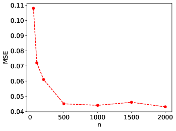
(a) Test-set MSE w.r.t. second-stage sample size

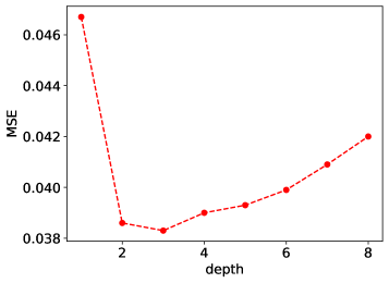
(b) Test-set MSE w.r.t. depth of KEFNN

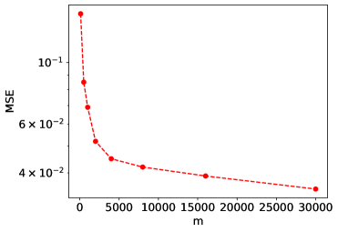
(c) Test-set MSE w.r.t. first-stage sample size

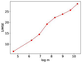
(d) Inverse of test-set MSE w.r.t. log of first-stage sample size

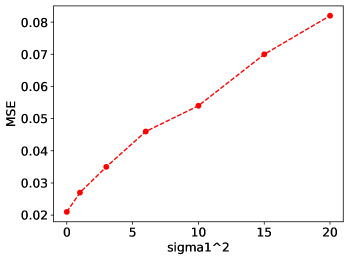
(e) Test-set MSE w.r.t. the variance of Gaussian noises in observations of input functions

(f) Test-set MSE w.r.t. the variance of Gaussian noises in observations of responses

Figure 1: The influence of second-stage sample size $n$, depth of KEFNN, first-stage sample size $m$, variances of noises in observations of input functions and responses on the test-set MSE.

In this subsection, we conduct numerical simulations to get further insights on our model and the theoretical results. Specifically, we consider the influence of different first-stage sample size $m$ and second-stage sample size $n$ on the generalization performance, as well as the influence of the noises in observations of input functions and responses on generalization performance. The target functional is chosen the same as case 3 in the above subsection, i.e., $Y=\langle f,\beta_{1}\rangle+(\langle f,\beta_{2}\rangle)^{2}$. Moreover, the hyperparameters in this subsection are chosen as the same, i.e., $\gamma=0.02$, $\beta=0.008$, $d_{1}=150$.

We first study the influence of the second-stage sample size $n$ on the generalization performance, where we use the first-stage sample size $m=4000$, and variances of noises $\sigma_{1}^{2}=3,\sigma_{2}^{2}=0.05$. It can be observed from Figure 1 (a) that the phase transition phenomenon of our model occurs at around $n=500$, i.e., the further increase on $n$ will not help the generalization performance. Comparing with the first-stage sample size $m$, such requirement on the second-stage sample size is very small, which is consistent with the theoretical results demonstrated in Section 4, owing to the utilization of the kernel embedding method with a smooth kernel.

Next, we study the influence of depth of our KEFNN on the generalization performance in the under-parameterized regime as is considered in the generalization analysis in Section 4. We use the first-stage sample size $m=5000$, second-stage sample size $n=500$, and variances of noises $\sigma_{1}^{2}=3,\sigma_{2}^{2}=0.05$. The width of deep neural network in our KEFNN is fixed to be 16, and it can be observed in Figure 1 (b) that with the increase of the depth, the generalization error first decreases and then increases, which is consistent with our generalization analysis that the generalization error is minimized when the number of nonzero parameters in KEFNN is of some particular rate w.r.t. the first-stage sample size. This partially instructs us how to conduct the model selection for our KEFNN.

In Figure 1 (c), we demonstrate the influence of first-stage sample size $m$ on the generalization performance, where we use the second-stage sample size $n=500$, and variances of noises $\sigma_{1}^{2}=3,\sigma_{2}^{2}=0.05$. To further indicate the decay rate of generalization error w.r.t. the increase of $m$, we display the inverse of test-set MSE w.r.t. $\log$ of first-stage sample size $m$ in Figure 1 (d). We can observe that the generalization error decays at a rate around $O((\log m)^{-1})$, i.e., a polynomial rate on $\log m$, this coincides with the learning rates derived in Section 4. Such polynomial rates on $\log m$ come from the unsatisfying rates of approximating nonlinear smooth functionals due to the curse of dimensionality. In order to achieve a generalization error $\epsilon$, we need to have $O(e^{1/\epsilon})$ first-stage sample size which is extremely large when $\epsilon$ is small. Therefore, it is an important issue to study under which circumstances we can overcome such curse of dimensionality for functional data.

Finally, we consider the effect of noises in observations of input functions and responses on generalization performance, the change of test-set MSE loss w.r.t. the variances of the Gaussian noises in observations of input functions and responses are presented in Figure 1 (c) and Figure 1 (d) respectively, where we use the first-stage sample size $m=4000$ and the second-stage sample size $n=500$, the variances of noises in responses are fixed as $\sigma_{2}^{2}=0$ for Figure 1 (c), and variances of noises in input functions are fixed as $\sigma_{1}^{2}=0$ for Figure 1 (d). It is quite interesting to notice that in both cases, the generalization error increases almost linearly w.r.t. the variances of the Gaussian noise in the observations. It could be further study to derive theoretical illustrations on such phenomenon. This also indicates that with kernel embedding as a pre-smoothing method, our functional net is quite robust to the noises in the observations of input functions, even when the second-stage sample size is not that large.

5.3 Examples on real functional datasets

In this subsection, we apply our KEFNN on some classical real functional datasets, and evaluate its performance by comparing with the baseline dimension reduction methods, i.e., ”Raw data”, ”B-spline”, and ”FPCA” methods followed by a deep neural network, with three hidden layers and 32 neurons in each layer. We do not compare with AdaFNN since the number of training samples is limited in these datasets and it does not perform well in some cases. The performance of the methods is measured by RMSE (root mean square error). The scores of dimension reduction by B-spline and FPCA are computed by using the functions in Python package ”scikit-fda” [37]. Moreover, the number of B-spline basis in ”B-spline”, number of eigenfunction basis in ”FPCA”, and hyperparameters in our KEFNN are all chosen based on the cross validation. We present the performance of functional deep neural networks with different dimension reduction methods on four learning tasks with real functional datasets in Table 2, with the mean and standard deviation of the test-set RMSE based on five training displayed.

Table 2: The test-set RMSE of functional deep neural network with different dimension reduction methods on four learning tasks with real functional datasets.

	Task 1	Task 2	Task 3	Task 4
Raw data+NN	0.2394 $\pm$ 0.010	0.1505 $\pm$ 0.007	0.2076 $\pm$ 0.028	0.1268 $\pm$ 0.013
B-spline+NN	0.2421 $\pm$ 0.003	0.1288 $\pm$ 0.010	0.2059 $\pm$ 0.010	0.1238 $\pm$ 0.033
FPCA+NN	0.2550 $\pm$ 0.085	0.1121 $\pm$ 0.015	0.1255 $\pm$ 0.015	0.1763 $\pm$ 0.023
KEFNN	0.2254 $\pm$ 0.002	0.0614 $\pm$ 0.003	0.1003 $\pm$ 0.011	0.1163 $\pm$ 0.013

In Task 1, we utilize the Medflies dataset in Python package ”scikit-fda”. The dataset includes 534 samples of Mediterranean fruit flies (Medfly), recording the number of eggs laid daily between day 5 and 34 for each fly. Our task is to utilize the early trajectory (first 20 days) of daily laid eggs to predict the whole reproduction of 30 days. In Task 2 and Task 3, we utilize the Tecator dataset in Python package ”scikit-fda”. The dataset includes 240 meat samples, for each meat sample the data consists of a 100 channel spectrum of absorbances and the contents of moisture (water), fat and protein. We aim at predicting the contents of fat and moisture of a meat sample in Task 2 and Task 3 respectively based on its spectrum of absorbances. In Task 4, we utilize the Moisture dataset in R package ”fds”. The dataset consists of near-infrared reflectance spectra of 100 wheat samples, measured in 2 nm intervals from 1100 to 2500nm, and the associated moisture content. Our task is to predict the moisture content a wheat sample based on its near-infrared reflectance spectra. In all the tasks, the train, validation, test split follows the ratio around 64:16:20. In Task 1, the hyperparameters in our KEFNN are chosen as $\gamma=0.033$, $\beta=0.01$, $d_{1}=100$. In the other three tasks, the hyperparameters are chosen as $\gamma=0.033$, $\beta=0.1$, $d_{1}=150$.

It can be observed from Table 2 that empirically our KEFNN consistently performs better than other baseline dimension reduction methods on various real functional datasets, this further demonstrates the advantage and flexibility of our method on learning different target functionals defined on various input function spaces. While none of the baseline methods can always perform better than other baseline methods in different learning tasks. Moreover, we notice that the standard deviation of RMSE for five training with our KEFNN is almost the smallest among these methods, indicating that our KEFNN is affected by randomness to a small extent. Therefore, the generalization error of the trained model tends to lie in a small interval with a higher probability.

Appendix

This appendix provides proof of the main results in Section 3 and Section 4, and some useful lemmas for the proof.

Appendix A Proof of Main Results

In this section, we prove the main results in this paper.

A.1 Proof of main results in Section 3

A.1.1 Proof of Theorem 1

Proof of Theorem 1.

Denote $\Xi_{d_{1}}$ as the space spanned by the basis $\{\phi_{1},\phi_{2},\dots,\phi_{d_{1}}\}$, and the isometric isomorphism $U_{d_{1}}:(\mathbb{R}^{d_{1}},\|\cdot\|_{2})\to(\Xi_{d_{1}},\|\cdot\|_{L_{2}(\mu)})$ as

$$U_{d_{1}}(v)=\sum_{i=1}^{d_{1}}v_{i}\phi_{i},\qquad v\in\mathbb{R}^{d_{1}}.$$ (A.1)

To prove the main results of approximation rates for the target functional $F$, the key is the following error decomposition with three terms to bound.

$$\sup_{f\in\mathcal{F}}|F(f)-F_{NN}(f)|$$ (A.2)

$$\leq \sup_{f\in\mathcal{F}}|F(f)-F(L_{K}f)|$$

$$+ \sup_{f\in\mathcal{F}}|F(L_{K}f)-F(U_{d_{1}}\circ T(L_{K}f))|$$

$$+ \sup_{f\in\mathcal{F}}|F\circ U_{d_{1}}(T(L_{K}f))-F_{NN}(f)|,$$

The first term focuses on the error of approximating the input function $f$ by its embedded function $L_{K}f$, the second term focuses on the error of approximating the embedded function $L_{K}f$ by its projection in the subspace spanned by the eigenfunction basis, and the final term focuses on the error of approximating a $\lambda$-Hölder continuous function by a deep ReLU neural network. We then bound these three error terms individually in the following.

For the first term, with the choice of the embedding kernel $K$ being (3.6), according to Lemma 1, $\forall f\in\mathcal{F}$,

$$\|f-L_{K}f\|_{L_{2}(\mu)}\leq C_{r}\|u\|_{L_{\infty}(\mathbb{R}^{d})}^{\frac{1}{2}}\omega_{r,L_{2}(\mathbb{R}^{d})}\left(f,\frac{\gamma}{\sqrt{2}}\right)\leq C_{d,r,\alpha}\gamma^{\alpha},$$

where $C_{d,r,\alpha}$ is a constant only depending on $d,r,\alpha,\mu$. Thus,

$$\sup_{f\in\mathcal{F}}|F(f)-F(L_{K}f)| \leq \sup_{f\in\mathcal{F}}C_{F}\|f-L_{K}f\|_{L_{2}(\mu)}^{\lambda}$$ (A.3)

$$\leq C_{F}C_{d,r,\alpha}^{\lambda}\gamma^{\alpha\lambda}.$$

For the second term, since $\forall f\in\mathcal{F}$, $L_{K}f\in\mathcal{H}_{\gamma}$, it can be written as $L_{K}f=\sum_{i=1}^{\infty}a_{i}\sqrt{\lambda_{i}}\phi_{i}$, with $\|L_{K}f\|_{H_{\gamma}}=\sqrt{\sum_{i=1}^{\infty}a_{i}^{2}}\leq(2^{r}-1)\pi^{-\frac{d}{4}}\gamma^{-\frac{d}{2}}$ by Lemma 1. Then

$$T(L_{K}f)=\left[a_{1}\sqrt{\lambda_{1}},a_{2}\sqrt{\lambda_{2}},\dots,a_{d_{1}}\sqrt{\lambda_{d_{1}}}\right],$$

$$U_{d_{1}}\circ T(L_{K}f)=\sum_{i=1}^{d_{1}}a_{i}\sqrt{\lambda_{i}}\phi_{i}.$$

It follows that

$$\left\|L_{K}f-U_{d_{1}}\circ T(L_{K}f)\right\|_{L_{2}(\mu)}^{2}=\left\|\sum_{i=d_{1}+1}^{\infty}a_{i}\sqrt{\lambda_{i}}\phi_{i}\right\|_{L_{2}(\mu)}^{2}$$

$$= \sum_{i=d_{1}+1}^{\infty}a_{i}^{2}\lambda_{i}\leq\lambda_{d_{1}+1}\sum_{i=d_{1}+1}^{\infty}a_{i}^{2}\leq\lambda_{d_{1}+1}\|L_{K}f\|_{H_{\gamma}}^{2}.$$

The eigenvalues of the one-dimensional Gaussian kernel have the following explicit formulation with exponential decay [18],

$$\lambda_{i}=\frac{\beta}{\gamma^{2i}\left(\frac{\beta^{2}}{2}\left(1+\sqrt{1+\left(\frac{2}{\beta\gamma}\right)^{2}}\right)+\frac{1}{\gamma^{2}}\right)^{i+\frac{1}{2}}}\leq\frac{\beta\gamma}{\left(1+\frac{\beta\gamma}{2}\right)^{2i+1}},$$

where $\mu$ is chosen as Gaussian distribution with $\beta$ being its bandwidth. We utilize such an explicit form since here the bandwidth $\gamma$ is a hyperparameter that needed to be carefully tuned later and cannot be viewed as a constant. Then the ${j+d\choose d}$-th eigenvalue of the multi-dimensional Gaussian kernel $k_{\gamma}$ is bounded by $\frac{(\beta\gamma)^{d}}{\left(1+\frac{\beta\gamma}{2}\right)^{2j+d}}$ [39]. Define ${j+d\choose d}\leq\frac{(j+\frac{d}{2})^{d}}{d!}=:d_{1}$, we have that the $d_{1}$-th eigenvalue of $k_{\gamma}$ is bounded by

$$\lambda_{d_{1}}\leq\frac{(\beta\gamma)^{d}}{\left(1+\frac{\beta\gamma}{2}\right)^{2c_{2}d_{1}^{\frac{1}{d}}}},$$ (A.4)

with $c_{2}=(d!)^{\frac{1}{d}}>\frac{d}{e}$ by Stirling’s theorem. Choose $\beta=2$, we get

$$\sup_{f\in\mathcal{F}}|F(L_{K}f)-F(U_{d_{1}}\circ T(L_{K}f))| \leq \sup_{f\in\mathcal{F}}C_{F}\|L_{K}f-U_{d_{1}}\circ T(L_{K}f)\|_{L_{2}(\mu)}^{\lambda}$$ (A.5)

$$\leq C_{F}C_{d,r,\lambda}\left(1+\gamma\right)^{-c_{2}\lambda d_{1}^{\frac{1}{d}}},$$

where $C_{d,r,\lambda}$ is a constant depending only on $d,r,\lambda$.

For the third term, since $F\circ U_{d_{1}}$ follows the smoothness of $F$, $\forall y_{1},y_{2}\in\mathbb{R}^{d_{1}}$,

$$|F\circ U_{d_{1}}(y_{1})-F\circ U_{d_{1}}(y_{2})| \leq C_{F}\|U_{d_{1}}(y_{1})-U_{d_{1}}(y_{2})\|_{L_{2}(\mu)}^{\lambda}$$ (A.6)

$$=C_{F}\|y_{1}-y_{2}\|_{2}^{\lambda},$$

it is essentially a $\lambda$-Hölder continuous function on $[-R,R]^{d_{1}}$ with $R=\|T(L_{K}f)\|_{\infty}$. Therefore, utilizing Lemma 2, there exists a deep ReLU neural network $H_{NN}$ with depth $d_{1}^{2}+d_{1}+1$, and $M$ nonzero parameters such that

$$\sup_{y\in[-R,R]^{d_{1}}}|F\circ U_{d_{1}}(y)-H_{NN}(y)|\leq 2C_{F}d_{1}\left(\frac{c_{0}d_{1}^{\frac{4}{d_{1}}}R}{M^{\frac{1}{d_{1}}}}\right)^{\lambda},$$

where $c_{0}$ is a constant independent of $d_{1},M$.

Recall the architecture of our functional net in Definition 1, it can be alternatively expressed as $F_{NN}(f)=H_{NN}\circ T(L_{K}f)$, where $H_{NN}$ is a standard deep ReLU neural network with input dimension $d_{1}$. Moreover, by Lemma 1 and the fact that $C_{K}=\tilde{c}_{0}\gamma^{-d}$ with $\tilde{c}_{0}$ being a positive constant, the radius of the input cube can be bounded by

$$R=\|T(L_{K}f)\|_{\infty}\leq\|L_{K}f\|_{L_{2}(\mu)}\leq C_{K}\mu(\mathbb{R}^{d})\|L_{K}f\|_{H_{\gamma}}\leq\tilde{c}_{0}\mu(\mathbb{R}^{d})(2^{r}-1)\pi^{-\frac{d}{4}}\gamma^{-\frac{3d}{2}},$$

Therefore, we conclude that there exists a functional net $F_{NN}$ following the architecture in Definition 1 with depth $J=d_{1}^{2}+d_{1}+2$ and $M$ nonzero parameters such that

$$\sup_{f\in\mathcal{F}}|F\circ U_{d_{1}}(T(L_{K}f))-F_{NN}(f)|\leq 2C_{F}d_{1}\left(\frac{c_{1}d_{1}^{\frac{4}{d_{1}}}\gamma^{-\frac{3d}{2}}}{M^{\frac{1}{d_{1}}}}\right)^{\lambda},$$ (A.7)

where $c_{1}$ is a constant independent of $d_{1},M$.

Finally, combining (A.3), (A.5), and (A.7), we have that

$$\sup_{f\in\mathcal{F}}|F(f)-F_{NN}(f)|\leq C_{F}C_{d,r,\alpha}^{\lambda}\gamma^{\alpha\lambda}+C_{F}C_{d,r,\lambda}\left(1+\gamma\right)^{-c_{2}\lambda d_{1}^{\frac{1}{d}}}+2C_{F}d_{1}\left(\frac{c_{1}d_{1}^{\frac{4}{d_{1}}}\gamma^{-\frac{3d}{2}}}{M^{\frac{1}{d_{1}}}}\right)^{\lambda},$$ (A.8)

To balance these three error terms, we can choose

$$d_{1}=\tilde{c}_{1}\frac{\log M}{\log\log M},\quad\gamma=\tilde{c}_{2}\left(\frac{\log\log M}{\log M}\right)^{\frac{1}{d}}\log\log M,$$ (A.9)

where $\tilde{c}_{1},\tilde{c}_{2}$ are positive constants that is determined later. Then for the first error

$$\gamma^{\alpha\lambda}=\tilde{c}_{2}^{\alpha\lambda}\left(\log M\right)^{-\frac{\alpha}{d}}\left(\log\log M\right)^{\left(\frac{1}{d}+1\right)\alpha\lambda},$$ (A.10)

since $(1+\frac{1}{x})^{x}\geq c_{3}$ with some constant $c_{3}\in(1,e)$ when $x$ is large enough, denote $x=\frac{1}{\gamma}$, then when $M$ is large enough, for the second error

$$\left(1+\gamma\right)^{-c_{2}\lambda d_{1}^{\frac{1}{d}}}=\left[(1+\frac{1}{x})^{x}\right]^{-c_{2}\tilde{c}_{1}^{\frac{1}{d}}\tilde{c}_{2}\lambda\log\log M}\leq\left(\log M\right)^{-c_{2}\tilde{c}_{1}^{\frac{1}{d}}\tilde{c}_{2}\lambda\log c_{3}},$$ (A.11)

finally, since $d_{1}^{\frac{4}{d_{1}}}\leq c_{4}$ for some constant $c_{4}$, and $M^{\frac{1}{d_{1}}}=(\log M)^{\frac{1}{\tilde{c}_{1}}}$, for the third error

$$d_{1}\left(\frac{c_{1}d_{1}^{\frac{4}{d_{1}}}\gamma^{-\frac{3d}{2}}}{M^{\frac{1}{d_{1}}}}\right)^{\lambda}\leq c_{1}^{\lambda}c_{4}^{\lambda}\tilde{c}_{1}\tilde{c}_{2}^{-\frac{3d\lambda}{2}}\left(\log M\right)^{\frac{3\lambda}{2}+1-\frac{\lambda}{\tilde{c}_{1}}}\left(\log\log M\right)^{-1-\frac{3(d+1)\lambda}{2}}.$$ (A.12)

Therefore, to balance (A.10), (A.11), and (A.12) w.r.t. the exponential rates on $\log M$, we can choose the constants

$$\tilde{c}_{1}<\frac{1}{\frac{3}{2}+\frac{\alpha}{d}+\frac{1}{\lambda}},\qquad\tilde{c}_{2}>\frac{\alpha}{dc_{2}\tilde{c}_{1}^{\frac{1}{d}}\log c_{3}},$$ (A.13)

thus we prove the desired bounds on the approximation error and depth with the constants $\tilde{c}_{3}=2\tilde{c}_{1}^{2}+2$, and $\tilde{c}_{4}=C_{F}C_{d,r,\alpha}^{\lambda}\tilde{c}_{2}^{\alpha\lambda}+C_{F}C_{d,r,\lambda}+2C_{F}c_{1}^{\lambda}c_{4}^{\lambda}\tilde{c}_{1}\tilde{c}_{2}^{-\frac{3d\lambda}{2}}$. ∎

A.1.2 Proof of Theorem 2

Proof of Theorem 2.

The only difference of the functional net architecture here with that in Theorem 1 is the embedding step, where

$$L_{K}f(x)=\int_{\Omega}K(x,t)f(t)dt,\quad x\in\Omega.$$

Denote $\tilde{f}$ as the extension by zero of $f$ to $\mathbb{R}^{d}$, then

$$L_{K}\tilde{f}(x)=\int_{\mathbb{R}^{d}}K(x,t)\tilde{f}(t)dt,\quad x\in\mathbb{R}^{d},$$

and we have that $L_{K}f=(L_{K}\tilde{f})|_{\Omega}$, it follows that

$$\|f-L_{K}f\|_{L_{2}(\mu)}\leq\|\tilde{f}-L_{K}\tilde{f}\|_{L_{2}(\tilde{\mu})},$$

where $\mu=\tilde{\mu}|_{\Omega}$, and $\tilde{\mu}$ is chosen as the same Gaussian distribution in the proof of Theorem 1. Therefore, the rest just follows from the proof of Theorem 1. ∎

A.1.3 Proof of Theorem 3

Proof of Theorem 3.

Since in this case the domain of the target functional is only a Gaussian RKHS, roughly speaking, the first error in the proof of Theorem 1 vanishes, and only the last two error terms remain for the final result with the balance on the choice of $d_{1}$. Denote the mapping $V_{d_{1}}:(\mathbb{R}^{d_{1}},|\cdot|)\to(\Xi_{d_{1}},\|\cdot\|_{L_{2}(\mu)})$ as

$$V_{d_{1}}(v)=\sum_{i=1}^{d_{1}}\frac{v_{i}}{\lambda_{i}}\phi_{i},\qquad v\in\mathbb{R}^{d_{1}}.$$ (A.14)

Now the error decomposition contains only two errors,

$$\sup_{f\in\mathcal{F}}|F(f)-F_{NN}(f)|$$ (A.15)

$$\leq \sup_{f\in\mathcal{F}}|F(f)-F(V_{d_{1}}\circ T(L_{K}f))|$$

$$+ \sup_{f\in\mathcal{F}}|F\circ V_{d_{1}}(T(L_{K}f))-F_{NN}(f)|.$$

We first consider the first error. For any $f\in\mathcal{H}_{\gamma}$, denote $f=\sum_{i=1}^{\infty}a_{i}\sqrt{\lambda_{i}}\phi_{i}$, with $\|f\|_{H_{\gamma}}=\sqrt{\sum_{i=1}^{\infty}a_{i}^{2}}\leq 1$. Then by (2.6), we have

$$T(L_{K}f)=\left[a_{1}\lambda_{1}^{\frac{3}{2}},a_{2}\lambda_{2}^{\frac{3}{2}},\dots,a_{d_{1}}\lambda_{d_{1}}^{\frac{3}{2}}\right],$$

$$V_{d_{1}}\circ T(L_{K}f)=\sum_{i=1}^{d_{1}}a_{i}\sqrt{\lambda_{i}}\phi_{i}.$$

It follows that

$$\left\|f-V_{d_{1}}\circ T(L_{K}f)\right\|_{L_{2}(\mu)}^{2}=\left\|\sum_{i=d_{1}+1}^{\infty}a_{i}\sqrt{\lambda_{i}}\phi_{i}\right\|_{L_{2}(\mu)}^{2}$$

$$= \sum_{i=d_{1}+1}^{\infty}a_{i}^{2}\lambda_{i}\leq\lambda_{d_{1}+1}\sum_{i=d_{1}+1}^{\infty}a_{i}^{2}\leq\lambda_{d_{1}+1}\|f\|_{H_{\gamma}}^{2}.$$

Therefore, by utilizing eigenvalue upper bound of Gaussian kernel, the first error is bounded by

$$\sup_{f\in\mathcal{F}}|F(f)-F(V_{d_{1}}\circ T(L_{K}f))| \leq \sup_{f\in\mathcal{F}}C_{F}\|f-V_{d_{1}}\circ T(L_{K}f)\|_{L_{2}(\mu)}^{\lambda}$$ (A.16)

$$\leq C_{F}C_{d,\gamma,\lambda}e^{-c_{2}\lambda d_{1}^{\frac{1}{d}}},$$

where $C_{d,\gamma,\lambda}$ is a constant depending only on $d,\gamma,\lambda$, and $c_{2}$ is a constant with $c_{2}>\frac{d}{e}$.

As for the second error, since $F\circ V_{d_{1}}$ follows the smoothness of $F$ with a scaling on the constant term,

$$|F\circ V_{d_{1}}(y_{1})-F\circ V_{d_{1}}(y_{1})| \leq C_{F}\|V_{d_{1}}(y_{1})-V_{d_{1}}(y_{2})\|_{L_{2}(\mu)}^{\lambda}$$ (A.17)

$$\leq\frac{C_{F}}{\lambda_{d_{1}}^{\lambda}}\|y_{1}-y_{2}\|_{2}^{\lambda},$$

Since the radius of the input for the deep ReLU neural network is bounded by

$$R =\|T(L_{K}f)\|_{\infty}\leq\|L_{K}f\|_{L_{2}(\mu)}\leq C_{K}\mu(\Omega)\|L_{K}f\|_{H_{\gamma}(\Omega)}$$

$$\leq\mu(\Omega)\left(\frac{\pi\gamma^{2}}{2}\right)^{\frac{d}{4}}\|f\|_{L_{2}(\Omega)}\leq\mu(\Omega)\left(\frac{\pi\gamma^{2}}{2}\right)^{\frac{d}{4}}\|f\|_{H_{\gamma}(\Omega)}\leq\mu(\Omega)\left(\frac{\pi\gamma^{2}}{2}\right)^{\frac{d}{4}},$$

where the third inequality is from [49, Proposition 4.46]. Therefore, same as the proof of Theorem 1, by Lemma 2, there exists a functional net $F_{NN}=H_{NN}\circ T(L_{K}f)$ in the form of Definition 1 with depth $J=d_{1}^{2}+d_{1}+2$ and number of nonzero parameters $M$ such that

$$\sup_{f\in\mathcal{F}}|F\circ V_{d_{1}}(T(L_{K}f))-F_{NN}(f)| \leq 2C_{F}\frac{d_{1}}{\lambda_{d_{1}}^{\lambda}}\left(\frac{c_{0}Rd_{1}^{\frac{4}{d_{1}}}}{M^{\frac{1}{d_{1}}}}\right)^{\lambda}$$ (A.18)

$$\leq c_{5}d_{1}e^{2c_{2}\lambda d_{1}^{\frac{1}{d}}}\left(\frac{d_{1}^{\frac{4}{d_{1}}}}{M^{\frac{1}{d_{1}}}}\right)^{\lambda},$$

where for the second inequality we utilize the eigenvalue lower bound of the Gaussian kernel, and $c_{5}$ is a positive constant depending on $c_{0},\gamma,d$.

Finally, combining (A.16) and (A.18), we have that

$$\sup_{f\in\mathcal{F}}|F(f)-F_{NN}(f)|\leq C_{F}C_{d,\gamma,\lambda}e^{-c_{2}\lambda d_{1}^{\frac{1}{d}}}+c_{5}d_{1}e^{2c_{2}\lambda d_{1}^{\frac{1}{d}}}\left(\frac{d_{1}^{\frac{4}{d_{1}}}}{M^{\frac{1}{d_{1}}}}\right)^{\lambda},$$ (A.19)

then choosing

$$d_{1}=c_{6}\left(\log M\right)^{\frac{d}{d+1}},$$ (A.20)

where $c_{6}$ is a constant to be determined later. For the first error, we have

$$e^{-c_{2}\lambda d_{1}^{\frac{1}{d}}}=e^{-c_{2}c_{6}^{\frac{1}{d}}\lambda\left(\log M\right)^{\frac{1}{d+1}}},$$ (A.21)

for the second error,

$$d_{1}e^{2c_{2}\lambda d_{1}^{\frac{1}{d}}}\left(\frac{d_{1}^{\frac{4}{d_{1}}}}{M^{\frac{1}{d_{1}}}}\right)^{\lambda}\leq c_{6}c_{4}^{\lambda}e^{\left(2c_{2}c_{6}^{\frac{1}{d}}-\frac{1}{c_{6}}\right)\lambda\left(\log M\right)^{\frac{1}{d+1}}}\left(\log M\right)^{\frac{d}{d+1}}.$$ (A.22)

Thus we can choose $c_{6}=(3c_{2})^{-\frac{d}{d+1}}$ to balance the dominated term of (A.21) and (A.22), then it follows that

$$\sup_{f\in\mathcal{F}}|F(f)-F_{NN}(f)|\leq\tilde{c}_{6}e^{-c_{7}\lambda\left(\log M\right)^{\frac{1}{d+1}}}\left(\log M\right)^{\frac{d}{d+1}},$$ (A.23)

with $\tilde{c}_{6}=C_{F}C_{d,\gamma,\lambda}+c_{5}c_{6}c_{4}^{\lambda}$, and

$$c_{7}=3^{-\frac{1}{d+1}}c_{2}^{\frac{d}{d+1}}>3^{-\frac{1}{d+1}}\left(\frac{d}{e}\right)^{\frac{d}{d+1}}>\left(\frac{d}{3e}\right)^{\frac{d}{d+1}}.$$ (A.24)

Thus we finish the proof with the constant $\tilde{c}_{5}=2c_{6}^{2}+2$. ∎

A.1.4 Proof of Theorem 4

Proof of Theorem 4.

The proof just follows from the proof of Theorem 3, with the only difference on the rates of eigenvalue decay. The upper bound of the eigenvalue was shown in [3], and we can derive the lower bound with the same method stated there, i.e., the eigenvalue decay of the integral operator associated with $K_{M}$ follows

$$C_{1}(\log k)^{2\alpha}k^{-2\alpha}\leq\lambda_{k}\leq C_{2}(\log k)^{2\alpha(d-1)}k^{-2\alpha},$$ (A.25)

where $C_{1},C_{2}$ are positive constants. According to the same error decomposition in the proof of Theorem 3, there exists a functional net $F_{NN}$ in the form of Definition 1 with depth $J=d_{1}^{2}+d_{1}+2$ and number of nonzero parameters $M$ such that

$$\sup_{f\in\mathcal{F}}|F(f)-F_{NN}(f)|\leq C_{F}C_{2}^{\frac{\lambda}{2}}(\log d_{1})^{\alpha\lambda(d-1)}{d_{1}}^{-\alpha\lambda}+C_{3}d_{1}^{2\alpha\lambda+1}(\log d_{1})^{-2\alpha\lambda}\left(\frac{d_{1}^{\frac{4}{d_{1}}}}{M^{\frac{1}{d_{1}}}}\right)^{\lambda},$$ (A.26)

where $C_{3}$ is a positive constant independent of $d_{1},M$. Finally, choose

$$d_{1}=C_{4}\frac{\log M}{\log\log M},$$ (A.27)

where $C_{4}$ is a constant that is determined later, for the first error

$$(\log d_{1})^{\alpha\lambda(d-1)}{d_{1}}^{-\alpha\lambda}\leq C_{4}^{-\alpha\lambda}\left(\log M\right)^{-\alpha\lambda}\left(\log\log M\right)^{\alpha\lambda(d-2)},$$ (A.28)

for the second error

$$d_{1}^{2\alpha\lambda+1}\left(\frac{d_{1}^{\frac{4}{d_{1}}}}{M^{\frac{1}{d_{1}}}}\right)^{\lambda}\leq c_{4}^{\lambda}C_{4}^{2\alpha\lambda+1}\left(\log M\right)^{2\alpha\lambda+1-\frac{\lambda}{C_{4}}}\left(\log\log M\right)^{-2\alpha\lambda-1},$$ (A.29)

thus we can choose $C_{4}\leq\frac{\lambda}{3\alpha\lambda+1}$ to balance (A.28) and (A.29) w.r.t. the dominated $\log M$ term. We thus get the desired bounds of depth and approximation error with the constants $C_{5}=2C_{4}^{2}+2$, and $C_{6}=C_{F}C_{2}^{\frac{\lambda}{2}}C_{4}^{-\alpha\lambda}+C_{3}c_{4}^{\lambda}C_{4}^{2\alpha\lambda+1}$. ∎

A.2 Proof of main results in Section 4

A.2.1 Proof of Proposition 1

Proof of Proposition 1.

$$|h(x)-h(y)| \leq\left|\sum\limits_{i=1}^{(N+1)^{d_{1}}}c_{i}\psi\left(\frac{N}{2R}(x-b_{i})\right)-\sum\limits_{i=1}^{(N+1)^{d_{1}}}c_{i}\psi\left(\frac{N}{2R}(y-b_{i})\right)\right|$$

$$\leq\sum\limits_{i=1}^{(N+1)^{d_{1}}}L\left|\psi\left(\frac{N}{2R}(x-b_{i})\right)-\psi\left(\frac{N}{2R}(y-b_{i})\right)\right|.$$

According to Lemma 3, we have

$$|\psi(x)-\psi(y)| \leq|\min\big{\{}\min_{k\neq j}(1+x_{k}-x_{j}),\min_{k}(1+x_{k}),\min_{k}(1-x_{k})\big{\}}$$

$$\quad-\min\big{\{}\min_{k\neq j}(1+y_{k}-y_{j}),\min_{k}(1+y_{k}),\min_{k}(1-y_{k})\big{\}}|$$

$$\leq 2(d_{1}^{2}+d_{1})||x-y||_{1}.$$

Therefore we have

$$|h(x)-h(y)| \leq\sum\limits_{i=1}^{(N+1)^{d_{1}}}2(d_{1}^{2}+d_{1})L\left|\left|\frac{N}{2R}(x-y)\right|\right|_{1}$$

$$\leq\frac{L}{R}N(N+1)^{d_{1}}(d_{1}^{2}+d_{1})||x-y||_{1},$$

which completes the proof by replacing $R$ with $C_{K}$. ∎

A.2.2 Proof of Proposition 2

Proof of Proposition 2.

Note that

$$\mathcal{E}\left(\pi_{L}F_{\widehat{D}}\right)-\mathcal{E}\left(F_{\rho}\right) =I_{1}+I_{2}+2\left\{\mathcal{E}_{D}\left(\pi_{L}F_{\widehat{D}}\right)-\mathcal{E}_{D}\left(\pi_{L}F_{D}\right)\right\}$$

$$\leq I_{1}+I_{2}+2\left\{\mathcal{E}_{D}\left(\pi_{L}F_{\widehat{D}}\right)-\mathcal{E}_{D}\left(\pi_{L}F_{D}\right)\right\}$$

$$\quad+2\left\{\mathcal{E}_{\widehat{D}}\left(\pi_{L}F_{D}\right)-\mathcal{E}_{\widehat{D}}\left(\pi_{L}F_{\widehat{D}}\right)\right\}.$$

The inequality from above holds since

$$\mathcal{E}_{\widehat{D}}\left(\pi_{L}F_{D}\right)\geq\mathcal{E}_{\widehat{D}}\left(F_{\widehat{D}}\right)\geq\mathcal{E}_{\widehat{D}}\left(\pi_{L}F_{\widehat{D}}\right).$$

The desired result is achieved by noting

$$2\left\{\mathcal{E}_{D}\left(\pi_{L}F_{\widehat{D}}\right)-\mathcal{E}_{D}\left(\pi_{L}F_{D}\right)\right\}+2\left\{\mathcal{E}_{\widehat{D}}\left(\pi_{L}F_{D}\right)-\mathcal{E}_{\widehat{D}}\left(\pi_{L}F_{\widehat{D}}\right)\right\}$$

$$\leq 2\left|\frac{1}{m}\sum_{i=1}^{m}(\pi_{L}H_{\widehat{D}}(u_{i})-y_{i})^{2}-\frac{1}{m}\sum_{i=1}^{m}(\pi_{L}H_{\widehat{D}}(\hat{u}_{i})-y_{i})^{2}\right|$$

$$+2\left|\frac{1}{m}\sum_{i=1}^{m}(\pi_{L}H_{D}(u_{i})-y_{i})^{2}-\frac{1}{m}\sum_{i=1}^{m}(\pi_{L}H_{D}(\hat{u}_{i})-y_{i})^{2}\right|$$

$$\leq 16L\sup_{H\in\mathcal{H}}\frac{1}{m}\sum_{i=1}^{m}\left|\pi_{L}H(u_{i})-\pi_{L}H(\hat{u}_{i})\right|$$

$$\leq 16L\sup_{H\in\mathcal{H}}\frac{1}{m}\sum_{i=1}^{m}\left|H(u_{i})-H(\hat{u}_{i})\right|=I_{3},$$

where the last inequality above is from $|\pi_{L}H(u_{i})-\pi_{L}H(\hat{u}_{i})|\leq|H(u_{i})-H(\hat{u}_{i})|$. ∎

A.2.3 Proof of Theorem 5

Proof of Theorem 5.

From Proposition 2, we know it suffices to bound the expectation of $I_{1}$, $I_{2}$ and $I_{3}$ separately.

• First, we derive a bound for $I_{1}$ in a probability form. Denote $\pi_{L}\mathcal{H}\circ L_{K}=\{\pi_{L}H\circ L_{K}:H\in\mathcal{H}\}$. For any $\epsilon>0$,

  $$P\left\{I_{1}>\epsilon\right\}$$

  $$= P\left\{||\pi_{L}F_{\widehat{D}}-F_{\rho}||_{\rho}^{2}-\left(\mathcal{E}_{D}(\pi_{L}F_{\widehat{D}})-\mathcal{E}_{D}({F_{\rho}})\right)>\frac{1}{2}\left(\epsilon+||\pi_{L}F_{\widehat{D}}-F_{\rho}||_{\rho}^{2}\right)\right\}$$

  $$\leq P\bigg{\{}\exists F\in\pi_{L}\mathcal{H}\circ L_{K}:||F-F_{\rho}||_{\rho}^{2}-\left(\mathcal{E}_{D}(F)-\mathcal{E}_{D}({F_{\rho}})\right)$$

  $$\quad>\frac{1}{2}\left(\frac{\epsilon}{2}+\frac{\epsilon}{2}+||F-F_{\rho}||_{\rho}^{2}\right)\bigg{\}}$$

  $$\leq 14\sup_{f_{1}^{m}}\mathcal{N}_{1}\left(\frac{\epsilon}{80L},\pi_{L}\mathcal{H}\circ L_{K},f_{1}^{m}\right)\exp\left(-\frac{m\epsilon}{5136L^{4}}\right),$$

  where we have used Lemma 4 in deriving the last inequality with $\alpha=\beta=\frac{\epsilon}{2}$, and $\delta=\frac{1}{2}$. Therefore, for any $a\geq\frac{1}{m}$,

  $$EI_{1} \leq\int_{0}^{\infty}P\{I_{1}>u\}du\leq a+\int_{a}^{\infty}P\{I_{1}>u\}du$$

  $$\leq a+\int_{a}^{\infty}14\sup_{f_{1}^{m}}\mathcal{N}_{1}\left(\frac{1}{80Lm},\pi_{L}\mathcal{H}\circ L_{K},f_{1}^{m}\right)\exp\left(-\frac{mu}{5136L^{4}}\right)du$$

  $$\leq a+14\sup_{f_{1}^{m}}\mathcal{N}_{1}\left(\frac{1}{80Lm},\pi_{L}\mathcal{H}\circ L_{K},f_{1}^{m}\right)\frac{5136L^{4}}{m}\exp\left(-\frac{ma}{5136L^{4}}\right),$$

  which is minimized if we choose

  $$a=\frac{5136L^{4}}{m}\log\left(14\sup_{f_{1}^{m}}\mathcal{N}_{1}\left(\frac{1}{80Lm},\pi_{L}\mathcal{H}\circ L_{K},f_{1}^{m}\right)\right),$$

  therefore, we have

  $$EI_{1} \leq\frac{5136L^{4}}{m}\left\{\log\left(14\sup_{f_{1}^{m}}\mathcal{N}_{1}\left(\frac{1}{80Lm},\pi_{L}\mathcal{H}\circ L_{K},f_{1}^{m}\right)\right)+1\right\}$$ (A.30)

  $$\leq\frac{5136L^{4}}{m}\left\{\log(28)+2c_{2}^{\prime}JM\log(M)\log(320eL^{2}m)+1\right\}$$

  $$\leq\frac{c^{\prime}_{1}JM\log M\log m}{m},$$

  where the second inequality above is from Lemma 5, and $c^{\prime}_{1}$ is a constant.

• Second, we estimate $EI_{2}$. Since $\mathcal{E}_{D}\left(\pi_{L}F_{D}\right)\leq\mathcal{E}_{D}\left(F_{D}\right)$, we have

  $$E{I_{2}} \leq 2E\left\{\mathcal{E}_{D}\left(F_{D}\right)-\mathcal{E}_{D}\left(F_{\rho}\right)\right\}$$ (A.31)

  $$=2E\left\{\inf_{F\in\{H\circ L_{K}:H\in\mathcal{H}\}}\mathcal{E}_{D}(F)-\mathcal{E}_{D}(F_{\rho})\right\}$$

  $$\leq 2\inf_{F\in\{H\circ L_{K}:H\in\mathcal{H}\}}E\left\{\mathcal{E}_{D}(F)-\mathcal{E}_{D}(F_{\rho})\right\}$$

  $$=2\inf_{F\in\{H\circ L_{K}:H\in\mathcal{H}\}}\|F-F_{\rho}\|_{\rho}^{2}.$$

• Third, we estimate $EI_{3}$. Note that

  $$EI_{3} =E\left\{16L\sup_{H\in\mathcal{H}}\frac{1}{m}\sum_{i=1}^{m}\left|H(u_{i})-H(\hat{u}_{i})\right|\right\}$$

  $$\leq E\left\{16L\frac{1}{m}\sum_{i=1}^{m}\sup_{H\in\mathcal{H}}\left|H(u_{i})-H(\hat{u}_{i})\right|\right\}$$

  $$\leq 16L\cdot E\left\{\sup_{H\in\mathcal{H}}\left|H(u_{1})-H(\hat{u}_{1})\right|\right\}.$$

  According to Proposition 1, we have

  $$\sup_{H\in\mathcal{H}}\left|H(u_{1})-H(\hat{u}_{1})\right|\leq\frac{L}{C_{K}}N(N+1)^{d_{1}}(d_{1}^{2}+d_{1})||Tu_{1}-T\hat{u}_{1}||_{1},$$

  Note that

  $$||Tu_{1}-T\hat{u}_{1}||_{1} =\sum_{i=1}^{d_{1}}\left|\int u_{1}(t)\phi_{i}(t)dt-\int\hat{u}_{1}(t)\phi_{i}(t)dt\right|$$

  $$\leq d_{1}||u_{1}-\hat{u}_{1}||_{L_{2}(\Omega)}.$$

  Therefore, we have

  $$EI_{3} \leq\frac{16L^{2}}{C_{K}}N(N+1)^{d_{1}}(d_{1}^{3}+d_{1}^{2})E\left(||u_{1}-\hat{u}_{1}||_{L_{2}(\Omega)}\right)$$

  $$\leq\frac{c^{\prime}_{5}}{C_{K}}M^{1+\frac{1}{d_{1}}}E\left(||u_{1}-\hat{u}_{1}||_{L_{2}(\Omega)}\right),$$

  where the last inequality is from (4.6), and $c^{\prime}_{5}$ is a constant depending on $C_{4}$ and $L$. By Lemma 6,

  $$E\left(||u_{1}-\hat{u}_{1}||_{L_{2}(\Omega)}\right)\leq\sqrt{\mu(\Omega)}C_{K_{0}}E\left(||u_{1}-\hat{u}_{1}||_{K_{0}}\right)\leq c^{\prime}_{6}\sqrt{\lambda_{q}},$$ (A.32)

  where $q=\frac{c^{\prime}_{5}n}{\log n}$, and $c^{\prime}_{6}$ is a positive constant. Note that this result also holds for embedding kernel $K$ being (3.6) as a linear combination of Gaussian kernels, and projection kernel $K_{0}=k_{\gamma}$. By triangle inequality, $||u_{1}-\hat{u}_{1}||_{L_{2}(\Omega)}$ can be bounded by a linear combination of $\|L_{K_{g}}f_{1}-\widehat{L_{K_{g}}}f_{1}\|_{L_{2}(\Omega)}$ with $K_{g}=k_{j\gamma}$, then we can apply Lemma 6 for each $K_{g}=k_{j\gamma}$ and use the fact that $\|\cdot\|_{K_{0}}\leq\|\cdot\|_{K_{g}}$, to get an upper bound of $||u_{1}-\hat{u}_{1}||_{K_{0}}$ by the eigenvalue decay of $K_{0}$, which is slower than eigenvalue decay of any $K_{g}=k_{j\gamma}$. Therefore, it follows that

  $$EI_{3}\leq\frac{c^{\prime}_{3}}{C_{K}}M^{1+\frac{1}{d_{1}}}\sqrt{\lambda_{q}},$$ (A.33)

  where $c^{\prime}_{3}=c^{\prime}_{5}c^{\prime}_{6}$.

Thus the proof is completed by combining (A.30), (A.31), and (A.33). ∎

A.2.4 Proof of Theorem 6

Proof of Theorem 6.

By Theorem 2, we know that there exists a functional net $F_{NN}$ with $M$ nonzero parameters, first hidden layer width $d_{1}=\tilde{c}_{1}\frac{\log M}{\log\log M}$, and depth $J\leq\tilde{c}_{3}\left(\frac{\log M}{\log\log M}\right)^{2}$, and embedding kernel being (3.6) with $\gamma=\tilde{c}_{2}\left(\frac{\log\log M}{\log M}\right)^{\frac{1}{d}}\log\log M\leq 1$ such that

$$\sup_{f\in\mathcal{F}}|F_{NN}(f)-F_{\rho}(f)|\leq\tilde{c}_{4}\left(\log M\right)^{-\frac{\alpha\lambda}{d}}\left(\log\log M\right)^{\left(\frac{1}{d}+1\right)\alpha\lambda},$$

then we have

$$\inf_{F\in\{H\circ L_{K}:H\in\mathcal{H}\}}\|F-F_{\rho}\|_{\rho}^{2} \leq||F_{NN}-F_{\rho}||_{\rho}^{2}\leq\sup_{f\in\mathcal{F}}|F_{NN}(f)-F_{\rho}(f)|^{2}$$ (A.34)

$$\leq\tilde{c}_{4}^{2}\left(\log M\right)^{-\frac{2\alpha\lambda}{d}}\left(\log\log M\right)^{2\left(\frac{1}{d}+1\right)\alpha\lambda}.$$

Plugging it into Theorem 5, since $M^{\frac{1}{d_{1}}}=(\log M)^{\frac{1}{\tilde{c}_{1}}}$, $\lambda_{q}\leq\hat{C}_{1}e^{-2c_{2}q^{\frac{1}{d}}}$, and $C_{K}=\tilde{c}_{0}\gamma^{-d}$ with $\tilde{c}_{0}$ being a positive constant, we get

$$\mathop{E}||\pi_{L}F_{\widehat{D}}-F_{\rho}||^{2}_{\rho}\leq \frac{c^{\prime}_{1}\tilde{c}_{3}M\log M\log m}{m}\left(\frac{\log M}{\log\log M}\right)^{2}$$ (A.35)

$$+\frac{c^{\prime}_{3}c^{\prime}_{4}}{\tilde{c}_{0}}\sqrt{\hat{C}_{1}}M(\log M)^{\frac{1}{\tilde{c}_{1}}}e^{-2c_{2}(\frac{c^{\prime}_{5}n}{\log n})^{\frac{1}{d}}}$$

$$+2\tilde{c}_{4}^{2}\left(\log M\right)^{-\frac{2\alpha\lambda}{d}}\left(\log\log M\right)^{2\left(\frac{1}{d}+1\right)\alpha\lambda}.$$

To balance the first and the third error term, we can choose the number of nonzero parameters in the functional net

$$M=\left\lfloor\frac{m}{(\log m)^{\frac{2\alpha\lambda}{d}+4}}\right\rfloor.$$ (A.36)

Then to make the second term has the same rate as other two terms, we can choose the second-stage sample size

$$n\geq\hat{C}_{2}(\log m)^{d}\log\log m,$$ (A.37)

with $\hat{C}_{2}$ being a positive constant large enough. When $m$ is large enough, we have that $(\frac{2\alpha\lambda}{d}+4)\log\log m\leq\tilde{C}_{1}\log m$ for some constant $\tilde{C}_{1}\in(0,1)$. Therefore we get the desired convergence rate with the constant $\tilde{C}_{2}=c^{\prime}_{1}\tilde{c}_{3}+c^{\prime}_{3}c^{\prime}_{4}\sqrt{\hat{C}_{1}}+2\tilde{c}_{4}^{2}(1-\tilde{C}_{1})^{-\frac{2\alpha\lambda}{d}}$. ∎

Appendix B Useful Lemmas

The following lemma showing the rates of approximating a function $f$ by its embedded function $L_{K}f$ is utilized in our approximation analysis, and can be found in [17, Theorem 2.2, Theorem 2.3].

Lemma 1.

Let $f\in L_{2}(\mathbb{R}^{d})\cap L_{\infty}(\mathbb{R}^{d})$, the embedding kernel $K$ is chosen as (3.6). Assume that $\mu$ is a measure on $\mathbb{R}^{d}$ with a Lebesgue density $u\in L_{\infty}(\mathbb{R}^{d})$. Then we have

$$\|f-L_{K}f\|_{L_{2}(\mu)}\leq C_{r}\|u\|_{L_{\infty}(\mathbb{R}^{d})}^{\frac{1}{2}}\omega_{r,L_{2}(\mathbb{R}^{d})}\left(f,\frac{\gamma}{\sqrt{2}}\right),$$ (B.1)

where $C_{r}$ is a constant only depending on $r$. Moreover, we have that $L_{K}f\in\mathcal{H}_{\gamma}(\mathbb{R}^{d})$, with

$$\|L_{K}f\|_{H_{\gamma}}\leq(2^{r}-1)\pi^{-\frac{d}{4}}\|f\|_{L_{2}(\mathbb{R}^{d})}\gamma^{-\frac{d}{2}}.$$ (B.2)

Next, we demonstrate a result from our previous work [47, Proposition 2] showing the rates of approximating a continuous function by a deep ReLU neural network, which essentially utilizes the idea of realizing the multivariate piecewise linear interpolation by a deep ReLU neural network from [58].

Lemma 2.

Let $M,N\in\mathbb{N}$, $\omega_{g}$ be the modulus of continuity of a function $g:[-R,R]^{d_{1}}\to[-L,L]$ with $L>0$, then there exists a deep ReLU neural network $H_{NN}$ with depth $d_{1}^{2}+d_{1}+1$, and $M$ nonzero parameters such that

$$\sup_{y\in[-R,R]^{d_{1}}}\left|g(y)-H_{NN}(y)\right|\leq 2d_{1}\omega_{g}\left(\frac{c_{0}d_{1}^{\frac{4}{d_{1}}}R}{M^{\frac{1}{d_{1}}}}\right),$$ (B.3)

where $c_{0}$ is a constant independent of $R,d_{1}$ and $M$. Moreover, $H_{NN}$ is constructed to output

$$H_{NN}(y)=\sum\limits_{i=1}^{(N+1)^{d_{1}}}c_{i}\psi\left(\frac{N}{2R}(y-b_{i})\right),$$ (B.4)

where $c_{i}\in\mathbb{R},b_{i}\in\mathbb{R}^{d_{1}}$ are free parameters depending on $g$, and satisfying $|c_{i}|\leq L$, $\|b_{i}\|_{\infty}\leq R$, $\psi:\mathbb{R}^{d}\to\mathbb{R}$ is defined as

$$\psi(y)=\sigma\Big{(}\min\big{\{}\min_{k\neq j}(1+y_{k}-y_{j}),\min_{k}(1+y_{k}),\min_{k}(1-y_{k})\big{\}}\Big{)}.$$ (B.5)

Furthermore, $N$ is the number of grid points in each direction, and have the following relationship with $M$,

$$C_{4}d_{1}^{4}(N+1)^{d_{1}}\leq M\leq C_{5}d_{1}^{4}(N+1)^{d_{1}},$$ (B.6)

for some constants $C_{4}$ and $C_{5}$.

The following lemma gives a bound of the difference between two $\min$ functions.

Lemma 3.

For any $k\in\mathbb{N}$, and any $x_{i},y_{i}\in\mathbb{R}$, $i=1,...,k$. Then there holds

$$\left|\min\{x_{1},...,x_{k}\}-\min\{y_{1},...,y_{k}\}\right|\leq 2\sum_{i=1}^{k}|x_{i}-y_{i}|.$$ (B.7)

Proof.

Note that for any $l\in\mathbb{N}$, we have $\min\{x_{1},...,x_{l}\}=x_{l}-\sigma(x_{l}-\min\{x_{1},...,x_{l-1}\})$, hence,

$$\left|\min\{x_{1},...,x_{k}\}-\min\{y_{1},...,y_{k}\}\right|$$

$$\leq\left|x_{k}-\sigma(x_{k}-\min\{x_{1},...,x_{k-1}\})-y_{k}+\sigma(y_{k}-\min\{y_{1},...,y_{k-1}\})\right|$$

$$\leq 2|x_{k}-y_{k}|+\left|\min\{x_{1},...,x_{k-1}\}-\min\{y_{1},...,y_{k-1}\}\right|$$

$$\leq\cdots$$

$$\leq 2|x_{k}-y_{k}|+...+2|x_{2}+y_{2}|+|x_{1}-y_{1}|$$

$$\leq 2\sum_{i=1}^{k}|x_{i}-y_{i}|,$$

which completes the proof. ∎

The following concentration inequality utilized in our generalization analysis can be found in [20, Theorem 11.4]. Although it only considered elements of $\mathcal{F}$ defined on $\mathbb{R}^{d}$, the result can also be applied to the case when elements of $\mathcal{F}$ is defined on an arbitrary set.

Lemma 4.

Let $m\in\mathbb{N}$, and assume $\rho(\{(f,y)\in\mathcal{Z}:|y|\leq L\})=1$ for some $L\geq 1$. Let $\mathcal{G}$ be a set of functions from $\mathcal{F}$ to $[-L,L]$. Then for any $0<\delta\leq 1/2$ and $\alpha,\beta>0$,

$$P\left\{\exists G\in\mathcal{G}:||G-F_{\rho}||^{2}_{\rho}-\left(\mathcal{E}_{D}(G)-\mathcal{E}_{D}(F_{\rho})\right)\geq\delta\left(\alpha+\beta+||G-F_{\rho}||^{2}_{\rho}\right)\right\}$$ (B.8)

$$\leq 14\sup_{f_{1}^{m}}\mathcal{N}_{1}\left(\frac{\beta\delta}{20L},\mathcal{G},f_{1}^{m}\right)\exp\left(-\frac{\delta^{2}(1-\delta)\alpha m}{214(1+\delta)L^{4}}\right).$$

The following lemma demonstrates the covering number bound of our functional net, and is utilized in the generalization analysis.

Lemma 5.

Let $\epsilon>0$, then for any $m\in\mathbb{N}$ and $f_{1},...,f_{m}\in\mathcal{F}$, we have

$$\mathcal{N}_{1}\left(\epsilon,\pi_{L}\mathcal{H}_{d_{1},M}\circ L_{K},f_{1}^{m}\right)\leq 2\left(\frac{4eL}{\epsilon}\right)^{c_{2}^{\prime}JM\log M},$$ (B.9)

where $J=d_{1}^{2}+d_{1}+1$, and $M$ is the number of nonzero parameters in the hypothesis space.

Proof.

For any functional class $\mathcal{H}$, [20, Lemma 9.2] shows a relationship between the $\epsilon$-covering number and the $\epsilon$-packing number,

$$\mathcal{N}_{1}\left(\epsilon,\mathcal{H},x_{1}^{m}\right)\leq\mathcal{M}_{1}\left(\epsilon,\mathcal{H},x_{1}^{m}\right).$$ (B.10)

Furthermore, denote $Pdim(\mathcal{H})$ as the pseudo-dimension of $\mathcal{H}$, which is the largest integer $N$ for which there exists $(x_{1},\dots,x_{N},y_{1},\dots,y_{N})\in\mathcal{X}^{N}\times\mathbb{R}^{N}$ such that for any $(a_{1},\dots,a_{N})\in\{0,1\}^{N}$, there exists some $h\in\mathcal{H}$ satisfying

$$h(x_{i})>y_{i}\Longleftrightarrow a_{i}=1,\qquad\forall i.$$

A relationship between the $\epsilon$-packing number and the pseudo-dimension was stated in [21, Theorem 6],

$$\mathcal{M}_{1}\left(\epsilon,\pi_{L}\mathcal{H},x_{1}^{m}\right)\leq\mathcal{M}_{1}\left(\epsilon,\mathcal{H},x_{1}^{m}\right)\leq 2\left(\frac{2eL}{\epsilon}\log\frac{2eL}{\epsilon}\right)^{Pdim(\mathcal{H})}.$$ (B.11)

Then, utilize the pseudo-dimension bound of the deep neural networks with any piecewise polynomial activation function including ReLU as a special case in [4, Theorem 7], we get a complexity bound for $\mathcal{H}_{NN}$, which is the class of deep ReLU networks $H_{NN}$ in the hypothesis space (4.3),

$$Pdim(\mathcal{H}_{NN})\leq c_{2}^{\prime}JM\log M,$$ (B.12)

where $J=d_{1}^{2}+d_{1}+1$, and $c_{2}^{\prime}$ is an absolute constant. Finally, since the nonzero parameters in $\pi_{L}\mathcal{H}_{d_{1},M}\circ L_{K}$ are only contained in $\mathcal{H}_{NN}$, combine (B.10), (B.11), and (B.12), we have

$$\mathcal{N}_{1}\left(\epsilon,\pi_{L}\mathcal{H}_{d_{1},M}\circ L_{K},f_{1}^{m}\right)=\mathcal{N}_{1}\left(\epsilon,\pi_{L}\mathcal{H}_{NN},x_{1}^{m}\right)\leq 2\left(\frac{4eL}{\epsilon}\right)^{c_{2}^{\prime}JM\log M},$$

where $x_{i}=T(L_{K}f_{i})$, for $i=1,\dots,m$. We thus prove the result. ∎

The following lemma states the convergences rate of the kernel quadrature with usage of the optimal quadrature scheme stated in Section 2 and can be found in [3]. Generally speaking, the convergence rates depend on the smoothness of the RKHS reproduced by the kernel, and can be measured by the eigenvalue decay of its integral operator.

Lemma 6.

Let $K$ be a Mercer kernel on $\Omega=[0,1]^{d}$ with eigensystem of the integral operator being $\{\lambda_{i},\phi_{i}\}$, where the eigenvalues are in the non-increasing order, and follow the polynomial or exponential decay. Then for the kernel embedding step (2.9), and its optimal quadrature scheme (2.10), we have

$$E\left(\left\|L_{K}f_{i}-\widehat{L_{K}}f_{i}\right\|_{K}\right)\leq c^{\prime}_{4}\sqrt{\lambda_{q}},$$ (B.13)

with $q=\frac{c^{\prime}_{5}n}{\log n}$, and $c^{\prime}_{4},c^{\prime}_{5}$ are positive constants.

References

• [1] Robert A Adams and John JF Fournier. Sobolev Spaces. Elsevier, 2003.
• [2] Anima Anandkumar, Kamyar Azizzadenesheli, Kaushik Bhattacharya, Nikola Kovachki, Zongyi Li, Burigede Liu, and Andrew Stuart. Neural operator: Graph kernel network for partial differential equations. In ICLR 2020 Workshop on Integration of Deep Neural Models and Differential Equations, 2020.
• [3] Francis Bach. On the equivalence between kernel quadrature rules and random feature expansions. The Journal of Machine Learning Research, 18(1):714–751, 2017.
• [4] Peter L Bartlett, Nick Harvey, Christopher Liaw, and Abbas Mehrabian. Nearly-tight VC-dimension and pseudodimension bounds for piecewise linear neural networks. The Journal of Machine Learning Research, 20(1):2285–2301, 2019.
• [5] Alain Berlinet and Christine Thomas-Agnan. Reproducing Kernel Hilbert Spaces in Probability and Statistics. Springer Science & Business Media, 2011.
• [6] Philippe Besse and James O Ramsay. Principal components analysis of sampled functions. Psychometrika, 51(2):285–311, 1986.
• [7] Kaushik Bhattacharya, Bamdad Hosseini, Nikola B Kovachki, and Andrew M Stuart. Model reduction and neural networks for parametric PDEs. The SMAI Journal of Computational Mathematics, 7:121–157, 2021.
• [8] Hervé Cardot, Frédéric Ferraty, and Pascal Sarda. Spline estimators for the functional linear model. Statistica Sinica, pages 571–591, 2003.
• [9] Tianping Chen and Hong Chen. Universal approximation to nonlinear operators by neural networks with arbitrary activation functions and its application to dynamical systems. IEEE Transactions on Neural Networks, 6(4):911–917, 1995.
• [10] Xiaming Chen, Bohao Tang, Jun Fan, and Xin Guo. Online gradient descent algorithms for functional data learning. Journal of Complexity, 70:101635, 2022.
• [11] Charles K Chui, Shao-Bo Lin, and Ding-Xuan Zhou. Deep neural networks for rotation-invariance approximation and learning. Analysis and Applications, 17(05):737–772, 2019.
• [12] Moo K Chung. Statistical and Computational Methods in Brain Image Analysis. CRC press, 2013.
• [13] Felipe Cucker and Steve Smale. On the mathematical foundations of learning. Bulletin of the American Mathematical Society, 39(1):1–49, 2002.
• [14] Felipe Cucker and Ding-Xuan Zhou. Learning Theory: An Approximation Theory Viewpoint, volume 24. Cambridge University Press, 2007.
• [15] Mo Deng, Shuai Li, Alexandre Goy, Iksung Kang, and George Barbastathis. Learning to synthesize: robust phase retrieval at low photon counts. Light: Science & Applications, 9(1):36, 2020.
• [16] Ronald A DeVore and George G Lorentz. Constructive Approximation, volume 303. Springer Science & Business Media, 1993.
• [17] Mona Eberts and Ingo Steinwart. Optimal regression rates for SVMs using Gaussian kernels. Electronic Journal of Statistics, 7:1–42, 2013.
• [18] Gregory E Fasshauer. Positive definite kernels: past, present and future. Dolomites Research Notes on Approximation, 4:21–63, 2011.
• [19] Frédéric Ferraty and Philippe Vieu. Nonparametric Functional Data Analysis: Theory and Practice, volume 76. New York: Springer, 2006.
• [20] László Györfi, Michael Köhler, Adam Krzyżak, and Harro Walk. A Distribution-Free Theory of Nonparametric Regression, volume 1. Springer, 2002.
• [21] David Haussler. Decision theoretic generalizations of the PAC model for neural net and other learning applications. Information and Computation, 100(1):78–150, 1992.
• [22] Yuehaw Khoo, Jianfeng Lu, and Lexing Ying. Solving parametric pde problems with artificial neural networks. European Journal of Applied Mathematics, 32(3):421–435, 2021.
• [23] Nikola Kovachki, Samuel Lanthaler, and Siddhartha Mishra. On universal approximation and error bounds for fourier neural operators. The Journal of Machine Learning Research, 22(1):13237–13312, 2021.
• [24] Samuel Lanthaler, Siddhartha Mishra, and George E Karniadakis. Error estimates for DeepONets: A deep learning framework in infinite dimensions. Transactions of Mathematics and Its Applications, 6(1):tnac001, 2022.
• [25] Zongyi Li, Nikola Kovachki, Kamyar Azizzadenesheli, Burigede Liu, Kaushik Bhattacharya, Andrew Stuart, and Anima Anandkumar. Fourier neural operator for parametric partial differential equations. In International Conference on Learning Representations, 2021.
• [26] Zongyi Li, Nikola Kovachki, Kamyar Azizzadenesheli, Burigede Liu, Andrew Stuart, Kaushik Bhattacharya, and Anima Anandkumar. Multipole graph neural operator for parametric partial differential equations. Advances in Neural Information Processing Systems, 33:6755–6766, 2020.
• [27] Lu Lu, Pengzhan Jin, Guofei Pang, Zhongqiang Zhang, and George Em Karniadakis. Learning nonlinear operators via DeepONet based on the universal approximation theorem of operators. Nature Machine Intelligence, 3(3):218–229, 2021.
• [28] Tong Mao, Zhongjie Shi, and Ding-Xuan Zhou. Theory of deep convolutional neural networks III: Approximating radial functions. Neural Networks, 144:778–790, 2021.
• [29] Tong Mao, Zhongjie Shi, and Ding-Xuan Zhou. Approximating functions with multi-features by deep convolutional neural networks. Analysis and Applications, pages 1–33, 2022.
• [30] Hrushikesh Narhar Mhaskar and Nahmwoo Hahm. Neural networks for functional approximation and system identification. Neural Computation, 9(1):143–159, 1997.
• [31] Hadrien Montanelli and Qiang Du. New error bounds for deep ReLU networks using sparse grids. SIAM Journal on Mathematics of Data Science, 1(1):78–92, 2019.
• [32] Yong Zheng Ong, Zuowei Shen, and Haizhao Yang. Integral autoencoder network for discretization-invariant learning. The Journal of Machine Learning Research, 23(286):1–45, 2022.
• [33] Allan Pinkus. N-widths in Approximation Theory, volume 7. Springer Science & Business Media, 2012.
• [34] William H Press, Saul A Teukolsky, William T Vetterling, and Brian P Flannery. Numerical Recipes in C. Cambridge University Press, 1992.
• [35] Chang Qiao, Di Li, Yuting Guo, Chong Liu, Tao Jiang, Qionghai Dai, and Dong Li. Evaluation and development of deep neural networks for image super-resolution in optical microscopy. Nature Methods, 18(2):194–202, 2021.
• [36] Zhen Qin, Qingliang Zeng, Yixin Zong, and Fan Xu. Image inpainting based on deep learning: A review. Displays, 69:102028, 2021.
• [37] Carlos Ramos-Carreño, José Luis Torrecilla, Miguel Carbajo-Berrocal, Pablo Marcos, and Alberto Suárez. scikit-fda: a Python package for functional data analysis. arXiv preprint arXiv:2211.02566, 2022.
• [38] J. O. Ramsay and B. W. Silverman. Functional Data Analysis. New York: Springer, 2005.
• [39] Carl Edward Rasmussen and Christopher K. I. Williams. Gaussian Processes for Machine Learning. MIT press, 2006.
• [40] John A Rice and Colin O Wu. Nonparametric mixed effects models for unequally sampled noisy curves. Biometrics, 57(1):253–259, 2001.
• [41] Fabrice Rossi and Brieuc Conan-Guez. Functional multi-layer perceptron: a non-linear tool for functional data analysis. Neural Networks, 18(1):45–60, 2005.
• [42] Fabrice Rossi, Brieuc Conan-Guez, and François Fleuret. Functional data analysis with multi layer perceptrons. In Proceedings of the 2002 International Joint Conference on Neural Networks. IJCNN’02 (Cat. No. 02CH37290), volume 3, pages 2843–2848. IEEE, 2002.
• [43] Fabrice Rossi, Nicolas Delannay, Brieuc Conan-Guez, and Michel Verleysen. Representation of functional data in neural networks. Neurocomputing, 64:183–210, 2005.
• [44] Johannes Schmidt-Hieber. Nonparametric regression using deep neural networks with ReLU activation function. The Annals of Statistics, 48(4):1875–1897, 2020.
• [45] Bernard W Silverman. Smoothed functional principal components analysis by choice of norm. The Annals of Statistics, 24(1):1–24, 1996.
• [46] Alex Smola, Arthur Gretton, Le Song, and Bernhard Schölkopf. A Hilbert space embedding for distributions. In Algorithmic Learning Theory, pages 13–31. Springer, 2007.
• [47] Linhao Song, Jun Fan, Di-Rong Chen, and Ding-Xuan Zhou. Approximation of nonlinear functionals using deep ReLU networks. arXiv preprint arXiv:2304.04443, 2023.
• [48] Linhao Song, Ying Liu, Jun Fan, and Ding-Xuan Zhou. Approximation of smooth functionals using deep ReLU networks. Neural Networks, 2022. Minor revision.
• [49] Ingo Steinwart and Andreas Christmann. Support Vector Machines. Springer Science & Business Media, 2008.
• [50] Taiji Suzuki. Adaptivity of deep ReLU network for learning in Besov and mixed smooth Besov spaces: optimal rate and curse of dimensionality. In International Conference on Learning Representations, 2019.
• [51] Matus Telgarsky. Benefits of depth in neural networks. In Conference on Learning Theory, pages 1517–1539. PMLR, 2016.
• [52] Chunwei Tian, Lunke Fei, Wenxian Zheng, Yong Xu, Wangmeng Zuo, and Chia-Wen Lin. Deep learning on image denoising: An overview. Neural Networks, 131:251–275, 2020.
• [53] Matt P Wand and M Chris Jones. Kernel Smoothing. CRC press, 1994.
• [54] Holger Wendland. Scattered Data Approximation, volume 17. Cambridge university press, 2004.
• [55] Fang Yao, Hans-Georg Müller, and Jane-Ling Wang. Functional data analysis for sparse longitudinal data. Journal of the American Statistical Association, 100(470):577–590, 2005.
• [56] Junwen Yao, Jonas Mueller, and Jane-Ling Wang. Deep learning for functional data analysis with adaptive basis layers. In International Conference on Machine Learning, pages 11898–11908. PMLR, 2021.
• [57] Dmitry Yarotsky. Error bounds for approximations with deep ReLU networks. Neural Networks, 94:103–114, 2017.
• [58] Dmitry Yarotsky. Optimal approximation of continuous functions by very deep ReLU networks. In Conference on Learning Theory, pages 639–649. PMLR, 2018.
• [59] Ding-Xuan Zhou. Universality of deep convolutional neural networks. Applied and Computational Harmonic Analysis, 48(2):787–794, 2020.
• [60] Hang Zhou, Fang Yao, and Huiming Zhang. Functional linear regression for discretely observed data: from ideal to reality. Biometrika, 2022.