Generation of massively entangled bright states of light during harmonic generation in resonant media

Abstract

At the fundamental level, full description of light-matter interaction requires quantum treatment of both matter and light. However, for standard light sources generating intense laser pulses carrying quadrillions of photons in a coherent state, classical description of light during intense laser-matter interaction has been expected to be adequate. Here we show how nonlinear optical response of matter can be controlled to generate dramatic deviations from this standard picture, including generation of multiple harmonics of the incident laser light entangled across many octaves. In particular, non-trivial quantum states of harmonics are generated as soon as one of the harmonics induces a transition between different laser-dressed states of the material system. Such transitions generate an entangled light-matter wavefunction, which emerges as the key condition for generating quantum states of harmonics, sufficient even in the absence of a quantum driving field or material correlations. In turn, entanglement of the material system with a single harmonic generates and controls entanglement between different harmonics. Hence, nonlinear media that are near-resonant with at least one of the harmonics appear to be most attractive for controlled generation of massively entangled quantum states of light. Our analysis opens remarkable opportunities at the interface of attosecond physics and quantum optics, with implications for quantum information science.

I Introduction

Quantum nature of light is central to our understanding of the micro-world, with the quantum description of the photo-electric effect ushering the new era in physics at the turn of the XX-th century. However, quantum description of light is typically used in the regime where just a few, or few tens, of photons interact with quantum matter. In contrast, when an intense incident light carries quadrillions of photons, counting each one of them individually is hardly expected to matter.

Recent observation [1] of the Schrödinger cat-type (so-called kitten) states and related statistics [2] of just such an intense light upon nonlinear-optical interaction with an atomic gas has upended this conventional wisdom. Granted, the observed Schrödinger kitten states have only emerged upon conditioning the observation of the transmitted driving field on detecting the highly nonlinear optical response to it. Nevertheless, Ref. [2, 1], followed by [3, 4, 5, 6, 7, 8, 9, 10], have opened an exciting possibility of using high harmonic emission to generate bright quantum states of light by measuring the transmitted laser field together with generated harmonics. Quantum properties of the generated light can be further amplified if the incident light interacts with a correlated quantum state of a material system, mapping quantum correlations of a pre-excited massively entangled, e.g. Dicke-like, state onto a quantum state of the generated light [11, 12, 13].

There is, of course, a different route to generating bright quantum states of light via nonlinear-optical response: begin with an intense incident light already in a quantum state [14, 15, 16]. As the quantum properties of the incident light should affect the quantum properties of the generated harmonics, the latter should emerge in nontrivial quantum states. The technological breakthrough in generating the so-called bright squeezed vacuum states of light [17, 18] with sufficient number of photons has enabled generation of several harmonics of this light [14].

Here we introduce a completely different avenue. We start with a standard laser pulse in a coherent state, and a quantum material system in a simple, uncorrelated ground state. To generate harmonics in a non-trivial quantum state, we rely only on the excitation of the material system by the generated harmonic light, a process often ignored in the description of high harmonic generation. Unsurprisingly, once such excitations are included, the light-matter state becomes entangled. This entanglement is central to what follows.

First, perhaps unexpectedly, all the components in the nonlinear optical response correlated to the new excited state of the material system become entangled with each other. Second, and most importantly, control over the excitations of the material system gives access to flexible control over the generated entangled states of light across multiple octaves. Third, such control over excitations in the material system needs to be neither complicated nor sophisticated: it can make use of the ubiquitous Stark shifts induced by the classical laser field, and be as straightforward as modulating the intensity envelope of the driving classical field.

Our analysis shows that generation of non-trivial quantum states of harmonics is not an exception: it should occur whenever the material system undergoes non-adiabatic transitions between its laser-dressed states. It does not need to rely on pre-exciting strongly correlated material states [12] or on using non-classical incident light [14, 15, 16]. As for conditioning the observations on a particular material response [2, 1, 13], this can also be effectively removed by shaping the transverse modes of the generated harmonics as discussed below.

We begin our analysis by first identifying the conditions that preclude generation of nontrivial quantum states of multiple harmonics. This helps us identify the key conditions for generating highly non-classical states of harmonics, starting with a purely classical incident light and a simple material system residing in an uncorrelated ground state. We then discuss one route to implementing these conditions, which to a theorist’s eye appears relatively straightforward.

II Prerequisites for generating quantum states of high harmonic light

The equation describing the interaction of light with a quantum system is (atomic units are used throughout):

$$i\frac{\partial}{\partial t}\ket{\Psi}=\hat{\textbf{H}}\Psi=\left[\hat{\textbf{H}}_{A}+\hat{\textbf{x}}\hat{\textbf{F}}+\hat{\textbf{H}}_{F}\right]\ket{\Psi},$$ (1)

where $\hat{H}_{A}$ is the Hamiltonian of the material system, $\hat{H}_{F}$ is the Hamiltonian of the quantum field, and $\hat{\textbf{x}}\hat{\textbf{F}}$ describes their coupling in the dipole approximation, with $\hat{\textbf{x}}$ representing the negative of the dipole operator; $\hat{\textbf{F}}$ is the electric field operator acting on all light modes, here characterized by their frequencies $\omega_{n}=n\omega$, with $\omega$ the incident frequency and $n=2k+1$ describing its odd harmonics. The wavefunction starts in the product state $\ket{\Psi_{0}}=\ket{g}\ket{\alpha_{\omega}}$, with $\ket{g}$ the field-free ground state of the material system and $\ket{\alpha_{\omega}}$ the initial coherent state at the fundamental frequency $\omega$.

What happens if the full wavefunction $\ket{\Psi(t)}$ remains, throughout the whole evolution, in the product state of the material system $\ket{\psi_{g}(t)}$ and the state of light $\ket{\chi_{{}_{F}}(t)}$, $\ket{\Psi(t)}=\ket{\psi_{g}(t)}\ket{\chi_{{}_{F}}(t)}$? Here the dressed quantum state of the material system $\ket{\psi_{g}(t)}$ has evolved from the field-free ground state and can include all states: ground, bound, and continuum; its final overlap with the ground state might even be negligible.

Substituting the ansatz $\ket{\Psi(t)}=\ket{\psi_{g}(t)}\ket{\chi_{{}_{F}}(t)}$ into the Eq.(1) yields the following equation for the quantum light field,

$$i\ket{\dot{\chi}_{{}_{F}}(t)}= \left[\hat{H}_{F}+\textbf{x}_{gg}(t)\hat{\textbf{F}}+\Delta E_{g}(t)\right]\ket{\chi_{{}_{F}}(t)},$$ (2)

where $\textbf{x}_{gg}(t)=\bra{\psi_{g}(t)}\hat{\textbf{x}}\ket{\psi_{g}(t)}$ is the dipole induced in the material system; the time-dependent energy shift in the material system $\Delta E_{g}(t)=\bra{\psi_{g}(t)}\hat{H}_{A}-i\frac{\partial}{\partial t}\ket{\psi_{g}(t)}$ has no influence on the quantum state of light $|\chi_{F}\rangle$, which starts in the product of vacuum states for each harmonic $n\omega$. Similar equation obtains for the material system.

For each $n\omega$, Eq.(2) describes a harmonic oscillator $\hat{H}_{F,n}$ starting in its ground state and driven by the time-dependent force $\textbf{x}_{gg}(t)$. No matter how complex $\textbf{x}_{gg}(t)$ is, the linear coupling $\textbf{x}_{gg}(t)\hat{\textbf{F}}$ can only shift the initial vacuum state $\ket{\alpha_{n}=0}$ to a coherent state $\ket{\alpha_{n}(t)}$ with a higher average photon number. The factorized nature of the initial state $\ket{\chi_{{}_{F}}}$, which starts as a product state of individual harmonics, each originally in its vacuum state, is preserved, as well as the maximally classical nature of the generated harmonics. What are the possible escape routes from this ”classical corner”, apart from those listed in the introduction?

Mathematically, one route is to turn the linear Eq.(2) for the quantum state of a generated harmonic $n$ into nonlinear: the material response $\textbf{x}_{gg}(t)$ entering Eq.(2) for some harmonic $n$ should be sensitive to the state $\ket{\chi_{{}_{F},_{n}}}$ of this harmonic. This removes the curse of limiting the evolution of $\ket{\chi_{{}_{F},_{n}}}$ to a single coherent state.

Physically, the dependence of the material response on the generated harmonics implies that they can induce transitions in the material system and change its nonlinear response. Thus, the quantum states of matter and the state of light become correlated. The way to incorporate such correlation is to eschew the factorized ansatz $\ket{\Psi(t)}=\ket{\psi_{g}(t)}\ket{\chi_{{}_{F}}(t)}$, which brought us into the unwanted ”classical corner” in the first place, explicitly providing for the possibility of light-matter entanglement. Quantum correlations and feedback between the generated nonlinear optical response and the state of the material system are the basis for generating nontrivial quantum states of all harmonics.

To emphasize the lack of need for quantum light at the input, we shall replace the field operator at the fundamental frequency $\omega$ with the classical field $\textbf{F}_{\rm cl}(t)=\bra{\alpha_{1}(t)}\hat{\textbf{F}}_{\rm 1}\ket{\alpha_{1}(t)}$, approximating the full Hamiltonian as

$$\hat{\textbf{H}}\simeq\hat{\textbf{H}}_{A}+\hat{\textbf{x}}\textbf{F}_{\rm cl}(t)+\hat{\textbf{x}}\sum_{n\neq 1}\hat{\textbf{F}}_{n}+\sum_{n\neq 1}\hat{\textbf{H}}_{F,n},$$

$$\textbf{F}_{\rm cl}(t)=\bra{\alpha_{1}(t)}\hat{\textbf{F}}_{\rm 1}\ket{\alpha_{1}(t)}.$$ (3)

Such approximation is by no means necessary, as the general analysis is just as straightforward as that developed below, but it allows us to bring to the fore the key role of light-matter entanglement, which leads to the generation of quantum light at the output without any quantum light at the input.

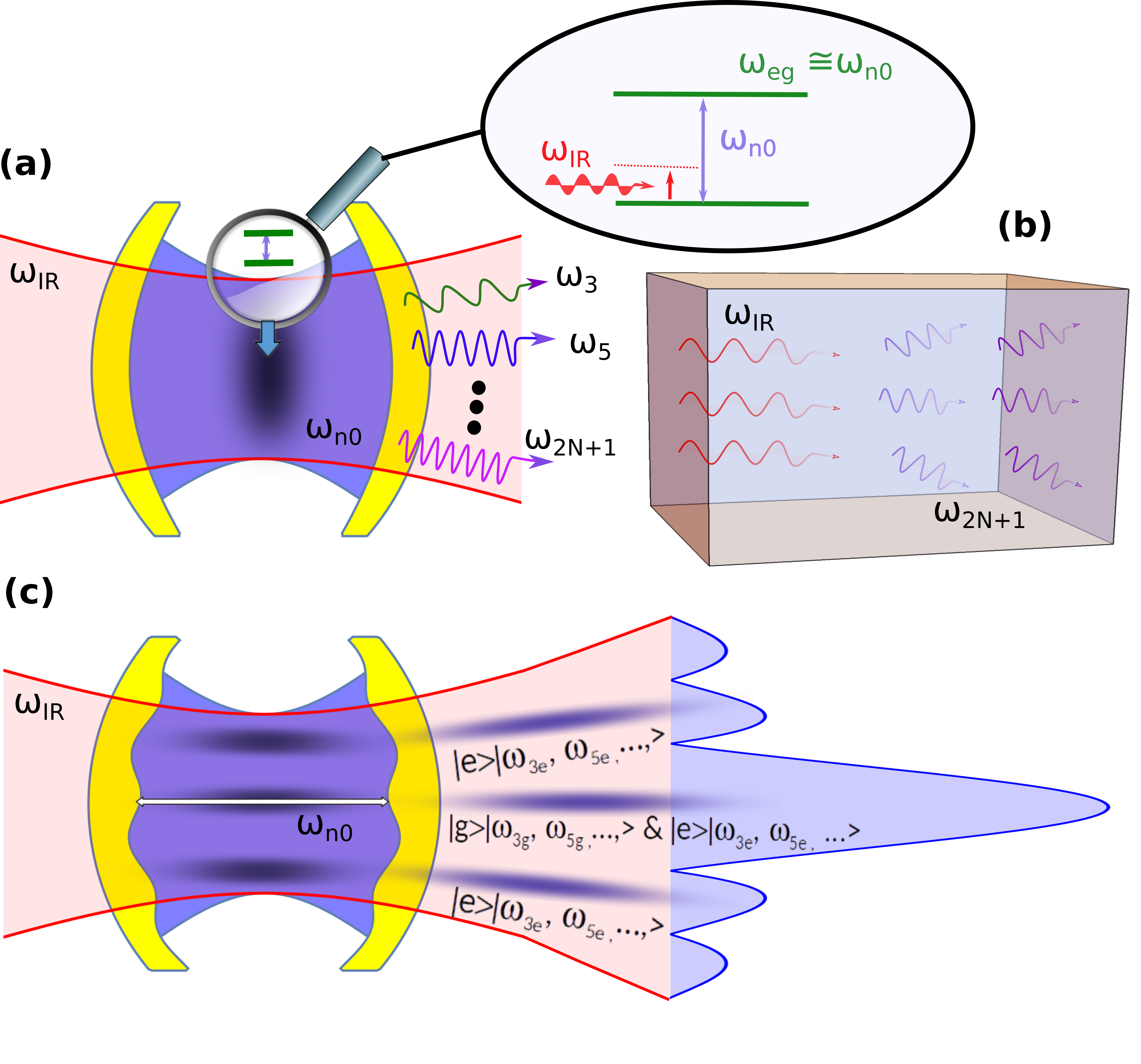
Figure 1: Some schemes for generating harmonics in quantum states. (a) Use of a cavity. Resonance between two laser-dressed states of a quantum system, driven by a low-frequency laser field, and a generated harmonic entangles the material system with the generated light. This also leads to massive entanglement between all harmonics generated upon the excitation. The resonance is enhanced by tuning the resonant cavity mode to the resonant harmonic. (b) Instead of the cavity, one can rely on absorption of some generated harmonic in a sufficiently dense medium. (c) Transverse shaping of the resonant cavity mode separates in the far field the highly non-classical components of the generated harmonics, correlated to the excited state, from the (less interesting) harmonics correlated to the ground state.

How can we enhance the feedback of the generated harmonic light on the material system that generates it? Given the relative weakness of generated harmonics, the most straightforward route is to ensure a one-photon resonance between some harmonic $n_{0}\omega$ and the transition between the ground $\ket{g}$ and some excited $\ket{e}$ state of the material system.

Importantly, this one-photon resonance does not have to be present at the zero fundamental field. On the contrary, we shall see below that it is beneficial to have such resonance induced by the Stark shifts of the ground and excited states.

To increase the light-matter coupling further, one can add a cavity resonant with $n_{0}\omega$, as shown in Fig.1(a). Fig. 1(b) shows a complementary option of an optically thick medium for some harmonics, which makes sure that these harmonics are invested in building the correlation between the state of the material system and the state of the generated light. Fig.1(c) shows that one can additionally shape the transverse mode of the generated resonant harmonic, separating in the far field all harmonics correlated to the excited state of the driven material system from those correlated to its ground state.

We shall see that resonant absorption of a single harmonic affects the quantum state of all other harmonics: single resonant transition is sufficient to dramatically affect quantum properties of all generated light fields.

III General formalism

One-photon resonance with a particular harmonic means that there is also an $n_{0}$-photon resonance with the fundamental field. Such multiphoton resonances can be already included in the definition of the laser-driven ground state $\ket{\psi_{g}(t)}$: we define $\ket{\psi_{g}(t)}$ as the solution of the time-dependent Schrödinger equation (TDSE) in the classical incident field $\textbf{F}_{\rm cl}(t)$, for the system starting in the ground state,

$$i\frac{\partial}{\partial t}\ket{\psi_{g}(t)}=\left[\hat{H}_{A}+\hat{\textbf{x}}\textbf{F}_{\rm cl}(t)\right]\ket{\psi_{g}(t)},$$

$$\ket{\psi_{g}(t_{i})}=\ket{g}.$$ (4)

We will refer to this state as the ”classically dressed” ground state. One-photon absorption of the harmonic $n_{0}\omega$ occurs between this state and the ”classically dressed” excited state $\ket{\psi_{e}(t)}$ defined as the solution of the standard semi-classical TDSE

$$i\frac{\partial}{\partial t}\ket{\psi_{e}(t)}=\left[\hat{H}_{A}+\hat{\textbf{x}}\textbf{F}_{\rm cl}(t)\right]\ket{\psi_{e}(t)},$$

$$\ket{\psi_{e}(t_{i})}=\ket{e}.$$ (5)

with the initial condition set to the excited field-free state $\ket{e}$. Note that these dressed states fully incorporate the incident field, remain orthogonal to each other, and offer a perfect basis to incorporate effects of the harmonics on the material system.

We can now write the full light-matter wavefunction as:

$$\ket{\Psi(t)}=\ket{\psi_{g}(t)}\ket{\chi_{g}(t)}+\sum_{e}\ket{\psi_{e}(t)}\ket{\chi_{e}(t)},$$ (6)

where $\ket{\chi_{g}(t)},\ket{\chi_{e}(t)}$ are the states of light correlated to the classically dressed states of the material system. Standard semi-classical treatment of intense light-matter interaction of the quantum material system with any classical field is limited to the single first term in the above equation. The second term is responsible for all the new aspects. To simplify the expressions that follow, we shall omit the summation over all dressed excited states and only keep the resonant contribution; restoring the full sum is straightforward.

Substituting Eq.(6) into the full Schrödinger equation yields coupled equations for the light fields correlated to the two strongly driven states of the material system,

$$i\ket{\dot{\chi}_{g}}= \hat{H}_{F}|\chi_{g}\rangle+\textbf{x}_{gg}(t)\hat{\textbf{F}}\ket{\chi_{g}}+\textbf{x}_{ge}(t)\hat{\textbf{F}}\ket{\chi_{e}},$$ (7)

$$i\ket{\dot{\chi}_{e}}= \hat{H}_{F}\ket{\chi_{e}}+\textbf{x}_{ee}(t)\hat{\textbf{F}}\ket{\chi_{e}}+\textbf{x}_{eg}(t)\hat{\textbf{F}}\ket{\chi_{g}},$$ (8)

where $\hat{\textbf{F}}=\sum_{n>1}\hat{\textbf{F}}_{n}$ is the field operator acting on all harmonics with orders $n\neq 1$,

$$\textbf{x}_{gg}(t)= \bra{\psi_{g}(t)}\hat{\textbf{x}}\ket{\psi_{g}(t)},$$

$$\textbf{x}_{ee}(t)= \bra{\psi_{e}(t)}\hat{\textbf{x}}\ket{\psi_{e}(t)},$$ (9)

are the laser-induced dipole in the dressed ground and excited states, and

$$\textbf{x}_{ge}(t)= \bra{\psi_{g}(t)}\hat{\textbf{x}}\ket{\psi_{e}(t)},$$

$$\textbf{x}_{eg}(t)= \bra{\psi_{e}(t)}\hat{\textbf{x}}\ket{\psi_{g}(t)},$$ (10)

describe the transition dipole matrix elements between the classically dressed states. In the limit of weak driving, they coincide with the usual transition dipoles between the field-free states and keep track of the transition frequency $\omega_{eg}=E_{e}-E_{g}$,

$$\textbf{x}_{eg}(t)=\bra{\psi_{e}(t)}\hat{\textbf{x}}\ket{\psi_{g}(t)}\rightarrow\textbf{x}_{eg}e^{i\omega_{eg}(t-t_{i})},$$ (11)

with $t_{i}$ some initial moment of time. In stronger fields, these transition dipoles can acquire non-trivial time-dependence, e.g. through the time-dependence of the transition frequency $\omega_{eg}(t)=E_{e}(t)-E_{g}(t)$ which incorporates the Stark shifts of both states. We shall take advantage of this ubiquitous effect below.

Addition of the couplings between different quantum states of light correlated to different dressed states of matter is central to turning what is usually a trivial evolution of the coherent states of all harmonics into an evolution generating non-trivial quantum states of multiple entangled harmonics.

We now take advantage of the interaction picture, defining $|\chi_{g,e}(t)\rangle=e^{-i\hat{H}_{F}t}|\phi_{g,e}(t)\rangle$. With this substitution, we have

$$i\ket{\dot{\phi}_{g}(t)}= \textbf{x}_{gg}(t)\hat{\textbf{F}}_{I}(t)\ket{\phi_{g}}+\textbf{x}_{ge}(t)\hat{\textbf{F}}_{I}(t)\ket{\phi_{e}},$$

$$i\ket{\dot{\phi}_{e}(t)}= \textbf{x}_{ee}(t)\hat{\textbf{F}}_{I}(t)\ket{\phi_{e}}+\textbf{x}_{eg}(t)\hat{\textbf{F}}_{I}(t)\ket{\phi_{g}},$$ (12)

where the time dependence of the operator $\hat{\textbf{F}}_{I}(t)$ is given by the transformation of the creation and annihilation operators for each frequency $n\omega$, e.g. $\hat{a}_{{}_{I},_{n}}(t)=\hat{a}_{n}e^{-in\omega t}$. The definition of $\hat{\textbf{F}}_{n}$ in terms of $\hat{a}$, $\hat{a}^{\dagger}$ is fixed by setting the classical incident field $\textbf{F}_{\rm cl}(t)=\langle\alpha_{1}(t)|\hat{\textbf{F}}_{\rm 1}|\alpha_{1}(t)\rangle$. If we set $F_{\rm cl}(t)\propto\cos\omega t\propto e^{-i\omega t}+e^{+i\omega t}$, then in the interaction picture

$$\hat{\textbf{F}}_{1,I}(t)=\boldsymbol{\mathcal{F}}_{1}f_{1}(t)\left[\hat{a}^{\dagger}_{1}e^{+i\omega t}+\hat{a}_{1}e^{-i\omega t}\right],$$ (13)

where $\boldsymbol{\mathcal{F}}_{1}$ is the vacuum field amplitude for the fundamental, and we have added the envelope $f_{1}(t)$ to account for the finite pulse length, assuming a sufficiently long pulse. We then use the same convention for the field operators at all other relevant frequencies, with $\boldsymbol{\mathcal{F}}_{n}$ the vacuum field amplitude for the harmonic $n$.

The simplest route to move forward with the coupled equations Eq.(12) is to use the time-dependent perturbation theory. Its zero-order equation describes the light field correlated to the dressed ground state,

$$i\ket{\dot{\phi}_{g}^{(0)}(t)}=\textbf{x}_{gg}(t)\hat{\textbf{F}}_{I}(t)\ket{\phi_{g}^{(0)}(t)}$$ (14)

with the initial condition being the vacuum state for all harmonics. Its formal solution is $\ket{\phi_{g}^{(0)}(t)}=\hat{U}^{(0)}_{g}(t,t_{i})\ket{\phi_{g}^{(0)}(t_{i})}$ where $\hat{U}^{(0)}_{g}(t,t_{i})$ is the propagator for the homogeneous equation Eq.(14) with the driving function $\textbf{x}_{gg}(t)$. It is a product of propagators for each harmonic,

$$\hat{U}^{(0)}_{g}(t,t_{i})=\prod_{n}\hat{U}^{(0)}_{g,n}(t,t_{i}).$$ (15)

At any time $t$, the quantum state of generated harmonics remains a product state. Moreover, for each harmonic $n$ the propagator $\hat{U}^{(0)}_{g,n}(t,t_{i})$ simply shifts the initial vacuum state $|\alpha_{n}(t_{i})=0\rangle$ to the coherent state $|\alpha_{n}(t)\rangle$, $|\alpha_{n}(t)\rangle=\hat{U}^{(0)}_{g,n}(t,t_{i})|\alpha_{n}(t_{i})\rangle$, where

$$\alpha_{n}(t)=-i\boldsymbol{\mathcal{F}}_{n}\int_{t_{i}}^{t}d\tau\textbf{x}_{gg,n}(\tau).$$ (16)

Here $\textbf{x}_{gg,n}$ is the complex amplitude of the Fourier component of the full dipole response $\textbf{x}_{gg}(t)$ at the frequency $n\omega$. For convenience, we have retained the slow temporal dependence of the amplitudes $x_{gg,n}=x_{gg,n}(\tau)$ on the envelope of the driving laser pulse, assuming that the pulse includes sufficiently many oscillations under its envelope to separate the two time-scales: the sub-cycle scale of the individual oscillations and the multi-cycle scale of the envelope.

The zero-order solution is then substituted into the equation for the field correlated to the dressed excited state, yielding

$$|\phi_{e}^{(1)}(t)\rangle=$$ (17)

$$=-i\int dt^{\prime}\hat{U}^{(0)}_{e}(t,t^{\prime})\textbf{x}_{eg}(t^{\prime})\hat{\textbf{F}}_{I}(t^{\prime})\hat{U}^{(0)}_{g}(t^{\prime},t_{i})|\phi_{g}^{(0)}(t_{i})\rangle,$$

where the propagator $\hat{U}^{(0)}_{e}(t,\tau)$ solves the homogeneous equation similar to Eq.(14) but for the laser-induced dipole generated by the material system in the dressed excited state, $\textbf{x}_{ee}(t)$.

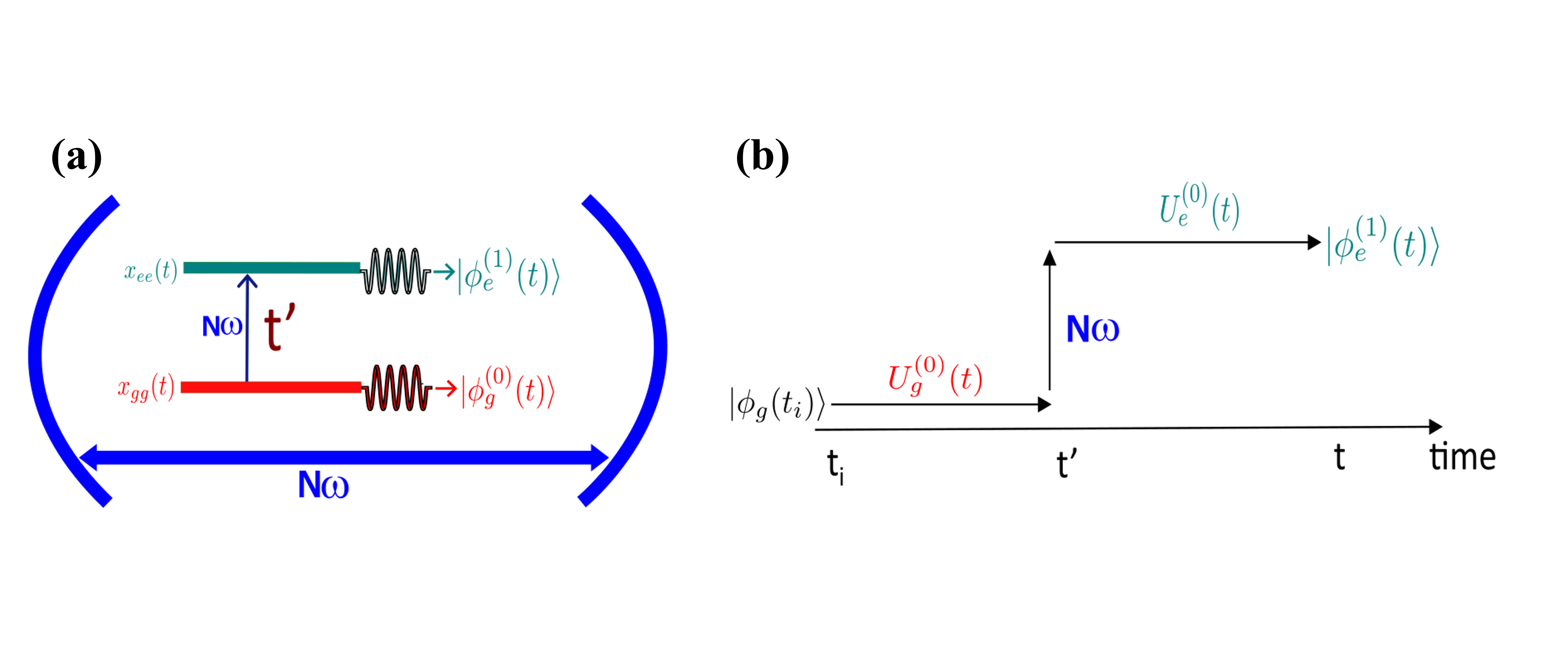
Figure 2: Generation of entangled harmonics correlated to the dressed excited state of the material system. (a) Resonant excitation, which can happen at any time $t^{\prime}$, alters the nonlinear material response and thus alters the generated product state of harmonics correlated to a specific excitation time $t^{\prime}$. The overall state $|\phi_{e}(t)\rangle$ is an integral, i.e. a sum, over all excitation times $t^{\prime}$, and is therefore no longer a product state. (b) The cartoon diagram describing the generation process, with the states of the harmonic fields evolving under the propagator $U_{g}^{(0)}$ from $t_{i}$ until $t^{\prime}$ and $U_{e}^{(0)}$ from $t^{\prime}$ to $t$. Since excitation can happen at any time, quantum mechanics demands summation over $t^{\prime}$, resulting in the sum over the product states, i.e. in an entangled state.

The physical meaning of this expression is simple and sketched in Figure 2. From the initial time $t_{i}$ until some instant $t^{\prime}$ the quantum fields at all harmonic frequencies are driven by the dipole response $\textbf{x}_{gg}(t)$ generated by the material system in its dressed ground state (which includes all dynamics induced by $\textbf{F}_{\rm cl}(t)$, possibly even the full depletion of the field-free ground state.) At an instant $t^{\prime}$ all quantum fields at all harmonics are ”lifted” by the operator $\textbf{x}_{eg}(t^{\prime})\hat{\textbf{F}}_{I}(t^{\prime})$ to the new electronic ”surface”, where they evolve from $t^{\prime}$ to $t$ driven by the dipole $\textbf{x}_{ee}(t)$ correlated to the dressed excited state.

Given the near-resonant (or resonant) condition for the harmonic $n_{0}\omega$, we shall use the resonant (rotating wave) approximation for the one-photon transition driven by this harmonic. This means that the full coupling term $\textbf{x}_{eg}(t^{\prime})\hat{\textbf{F}}_{I}(t^{\prime})$ is approximated by its resonant contribution,

$$\textbf{x}_{eg}(t^{\prime})\hat{\textbf{F}}_{I}(t^{\prime})\simeq\tilde{\textbf{x}}_{eg}e^{+i\int_{t_{i}}^{t^{\prime}}d\tau\omega_{eg}(\tau)}\boldsymbol{\mathcal{F}}_{n_{0}}\left[\hat{a}_{n_{0}}e^{-in_{0}\omega t^{\prime}}\right]=$$

$$=\tilde{\textbf{x}}_{eg}e^{+i\int_{t_{i}}^{t^{\prime}}d\tau\Delta_{eg}(\tau)}\boldsymbol{\mathcal{F}}_{n_{0}}\hat{a}_{n_{0}},$$ (18)

where the detuning of resonance $\Delta(t)=\omega_{eg}(t)-n_{0}\omega$ incorporates the Stark shifts of the classically dressed states, and $\tilde{\mathbf{x}}_{eg}$ is the dipole transition matrix element at the resonant frequency. This approximation assumes that electronic excitation between the dressed states is accompanied by annihilating the resonant photon $n_{0}\omega$. In principle, $\tilde{\mathbf{x}}_{eg}$ can retain a slow temporal dependence on the pulse envelope, $\tilde{\mathbf{x}}_{eg}(\tau)$, which incorporates additional distortions of the dressed states (beyond the simple Stark shift) induced by the driving field $\omega$.

The integrand in Eq.(17) can now be written in a simple form. Indeed, the initial quantum state of the harmonic light is a product of the vacuum states for all harmonics, the propagator $\hat{U_{g}}^{(0)}(t^{\prime},t_{i})$ is a product of linear zero-order propagators for each individual harmonic, and at $t^{\prime}$ the quantum state of light remains a product state, just as in the zero order discussed above. Moreover, just as in the zero order, for each harmonic $n$ the propagator $\hat{U}^{(0)}_{g,n}(t^{\prime},t_{i})$ simply shifts the vacuum state $|\alpha_{n}(t_{i})=0\rangle$ to the coherent state $|\alpha_{n}(t^{\prime})\rangle$ with

$$\alpha_{n}(t^{\prime})=-i\boldsymbol{\mathcal{F}}_{n}\int_{t_{i}}^{t^{\prime}}d\tau\textbf{x}_{gg,n}(\tau).$$ (19)

Next, we apply the transition operator Eq.(18) in Eq.(17). It leaves all $n\neq n_{0}$ undisturbed, while for $n=n_{0}$ it yields $\hat{a}_{n_{0}}|\alpha_{n_{0}}(t^{\prime},t_{i})\rangle=\alpha_{n_{0}}(t^{\prime})|\alpha_{n_{0}}(t^{\prime})\rangle$. Finally, the action of the propagator $\hat{U}^{(0)}_{e,n}(t,t^{\prime})$ on the coherent state $|\alpha_{n}(t^{\prime})\rangle$ yields another coherent state at the moment $t$, $\hat{U}^{(0)}_{e,n}(t,t^{\prime})|\alpha_{n}(t^{\prime})\rangle=|\alpha_{n}(t,t^{\prime})\rangle$, where

$$\alpha_{n}(t,t^{\prime})=$$ (20)

$$=-i\boldsymbol{\mathcal{F}}_{n}\left[\int_{t_{i}}^{t^{\prime}}d\tau\textbf{x}_{gg,n}(\tau)+\int_{t^{\prime}}^{t}d\tau\textbf{x}_{ee,n}(\tau)\right].$$

This yields the final result in the first-order perturbation theory with respect to the quantum feedback between the generated light and the material system,

$$|\phi_{e}^{(1)}(t)\rangle=$$ (21)

$$=-i\int dt^{\prime}\tilde{\textbf{x}}_{eg}(t^{\prime})e^{+i\int_{t_{i}}^{t^{\prime}}d\tau\Delta_{eg}(\tau)}\boldsymbol{\mathcal{F}}_{n_{0}}\alpha_{n_{0}}(t^{\prime})\prod_{n>1}|\alpha_{n}(t,t^{\prime})\rangle.$$

In general, the above result represents a massively entangled quantum state of light: indeed, the integral is a sum of the product states $\prod_{n>1}|\alpha_{n}(t,t^{\prime})\rangle$, with $t^{\prime}$ a continuous summation index.

Below we discuss several specific scenarios that realize different entangled states, demonstrating routes to control the resulting outcome. Note that all generated states emerge from coherent states characterized by their indices $\alpha_{n}$ Eq.(19). Thus, in what follows, we will characterize the generated states using the average photon numbers

$$N_{n}(T)=|\boldsymbol{\mathcal{F}}_{n}\int_{t_{i}}^{T}d\tau\textbf{x}_{gg,n}(\tau)|^{2}$$ (22)

that the coherent states at frequencies $\omega_{n}=n\omega$ would have acquired at the end of the laser pulse $T$, had the material system stayed in the dressed ground state throughout the whole laser pulse. We will use $N_{3}=N_{3}(T)$ for the third harmonic as the overall reference number. For other harmonics, the key numbers are then $N_{n}/N_{3}$, which are controlled by the parameters of the laser pulse and the cavity. For example, if $n=5$ is resonant with the cavity mode, the choice of the laser frequency, intensity, and the quality of the cavity can allow one to vary $N_{5}/N_{3}$ in a broad range. We shall also use $N_{n}(t)$ (for $t<T$) to denote the average number of photons in a coherent state $|\alpha_{n}\rangle$ that would have been generated by the material system in its dressed ground state by the time $t$ (given by the same equation Eq.(22) with $t$ in the upper limit of the integral.)

IV Results and Discussion

To appreciate the entangled nature of the generated harmonics state, and the possibility to control it, we begin by considering the so-called Freeman resonances [19, 20], where the conventional Stark shift proportional to the intensity of the classical IR driver brings the states in and out of resonance, as shown in Fig.3(a). The integral is now accumulated during the temporal windows near the resonant times $t_{k}$ and can be computed using the standard stationary phase method, yielding at the end of the laser pulse $T$

$$|\phi_{e}^{(1)}(T)\rangle=\sum_{k}C_{k}e^{+i\int_{t_{i}}^{t_{k}}d\tau\Delta_{eg}(\tau)}\prod_{n>1}|\alpha_{n}(T,t_{k})\rangle,$$

$$C_{k}=\sqrt{\frac{-2\pi i}{\dot{\Delta}_{eg}(t_{k})}}\tilde{\textbf{x}}_{eg}\boldsymbol{\mathcal{F}}_{n_{0}}\alpha_{n_{0}}(t_{k})\ .$$ (23)

Here $\dot{\Delta}_{eg}(t_{k})$ is the time-derivative of the resonance detuning at the moment of resonance $t_{k}$. The physical meaning of $C_{k}$ is nothing but the amplitude of one-photon excitation by the resonant harmonic $n_{0}$ during the resonance window $t_{k}$. Here, this amplitude is computed using first order perturbation theory and is proportional to $\boldsymbol{\mathcal{F}}_{n_{0}}\alpha_{n_{0}}(t_{k})$, which is simply the classical electric field amplitude $\mathbf{F}_{n_{0}}(t_{k})=\boldsymbol{\mathcal{F}}_{n_{0}}\alpha_{n_{0}}(t_{k})$ of the resonant harmonic $n_{0}\omega$ at the moment $t_{k}$. Naturally, the transition amplitude $C_{k}$ also includes the transition dipole matrix element $\tilde{\mathbf{x}}_{eg}$. This matrix element may change from its field-free value because the states $|\psi_{g}\rangle$ and $|\psi_{e}\rangle$ of the material system are dressed by the laser field. Therefore, it depends on the pulse envelope, and this dependence can be incorporated as $\tilde{\mathbf{x}}_{eg}=\tilde{\mathbf{x}}_{eg}(t_{k})$. The phase factors $e^{+i\int_{t_{i}}^{t_{k}}d\tau\Delta_{eg}(\tau)}$ control the relative phases between the terms in the sum. Overall, the amplitudes $C_{k}$ describe the non-adiabatic Landau-Zener-Dykhne transitions between the dressed states driven through the resonance, with the phase factors $e^{+i\int_{t_{i}}^{t_{k}}d\tau\Delta_{eg}(\tau)}$ responsible for the Stueckelberg oscillations (named so after Baron Ernst Carl Gerlach Stueckelberg von Breidenbach zu Breidenstein und Melsbach) in the final generated state, as the coherent states are not orthogonal. We stress again that both the number of the terms in the sum and the relative phases between them are controlled by shaping the intensity envelope of the fundamental laser pulse.

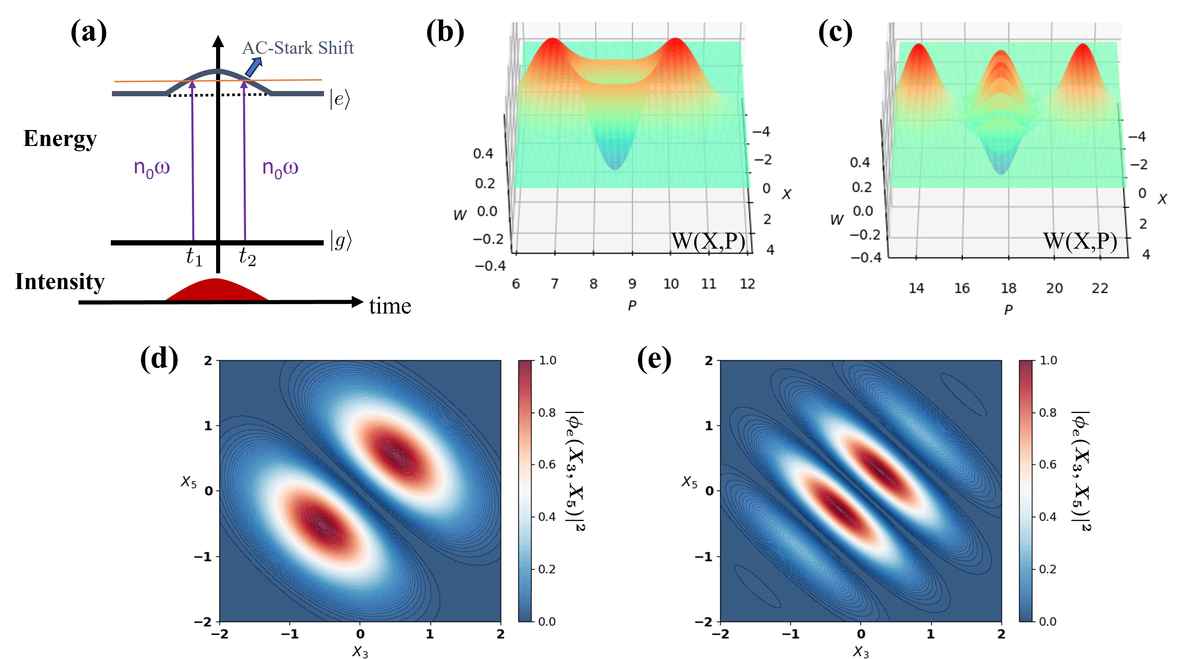
Figure 3: Control of resonances and of the generated quantum states of light. (a) Stark shift follows the intensity envelope of the driving laser field and brings the ground and excited states in resonance twice during the pulse. (b,c) Wigner function for one of the harmonics, here $n=3$, upon artificially removing its entanglement with others. For illustration, we set resonances at $t_{1}$ and $t_{2}$ to occur when the average number of the harmonic photons $N_{3}(t)$ generated by the laser-dressed ground state are $N_{3}(t_{1})=25$, $N_{3}(t_{2})=50$ (b) and $N_{3}(t_{1})=100$, $N_{3}(t_{2})=225$ (c). (d,e) Intensity of the $X$-quadratures of the entangled state of two harmonics, here $n=3$ and $n=5$, $|\phi_{e}(X_{3},X_{5})|^{2}$. The parameters are set to $N_{3}(t_{1})=N_{5}(t_{1})=25$, $N_{5}(t_{2})=N_{3}(t_{2})=50$ in (d) and $N_{3}(t_{1})=N_{5}(t_{1})=100$, $N_{5}(t_{2})=N_{3}(t_{2})=225$ in (e).

Examples of quantum states of light that can be created this way are shown in Fig.3, for two resonant windows and hence two terms in the sum. For simplicity of visual presentation, we assume that only two harmonics, the third (n=3) and the fifth (n=5), are efficiently generated, so that the entangled wavefunction contains only two terms in each product state,

$$\ket{\phi_{e}^{(1)}(T)}=$$

$$=C_{1}\ket{\alpha_{3}(T,t_{1})}\ket{\alpha_{5}(T,t_{1})}+C_{2}e^{i\Phi}\ket{\alpha_{3}(T,t_{2})}\ket{\alpha_{5}(T,t_{2})},$$

$$\Phi=\int_{t_{1}}^{t_{2}}d\tau\Delta_{eg}(\tau).$$ (24)

This constraint is only used for simplicity of visualizing the overall quantum state of light. Note that $\alpha_{n}$ and $\Phi$ are fully controlled by the parameters of the driving laser pulse and the parameters of the cavity.

To give an impression of the underlying structure of a single frequency mode, say $n=3$, we first artificially set $\alpha_{5}(T,t_{1})=\alpha_{5}(T,t_{2})$, which allows us to disentangle the third harmonic from the fifth and plot its Wigner function. The state is, clearly, a Schrödinger cat $\ket{\alpha_{3}(T,t_{1})}+e^{+i\Phi}\ket{\alpha_{3}(T,t_{2})}$. Fig.3 shows the Wigner functions of this cat state for the case of $\Phi=\pi$ and $N_{3}(t_{1})=25$, $N_{3}(t_{2})=50$ in panel (b) and $N_{3}(t_{1})=100$, $N_{3}(t_{2})=225$ in panel (c). Note that both the relative phase $\Phi$ and the photon numbers are fully controlled by the time delay between the resonances and the Stark shifts induced by the driving laser field. The characteristic non-classical features of the Schrödinger cat state are apparent in Figs. 3(b,c).

We next move to the example where both the third and the fifth harmonics are generated with similar efficiency. This could be achieved, for example, by tuning the cavity resonance close to the $n=5$ harmonic and staying within the perturbative regime with respect to the driving laser field, so that higher order harmonics are negligible. The 2D plot of the resulting state as a function of the x-quadratures $X_{3}$ and $X_{5}$ of both harmonics is shown in Fig.3(d), for $N_{3}(t_{1})=N_{5}(t_{1})=25$ and $N_{3}(t_{2})=N_{5}(t_{2})=50$, with equal amplitudes $|C_{1}|=|C_{2}|$ and the relative phase $\Phi=\pi$ between the two terms. Panel (e) shows the same for $N_{3}(t_{1})=N_{5}(t_{1})=100$ and $N_{3}(t_{2})=N_{5}(t_{2})=225$.

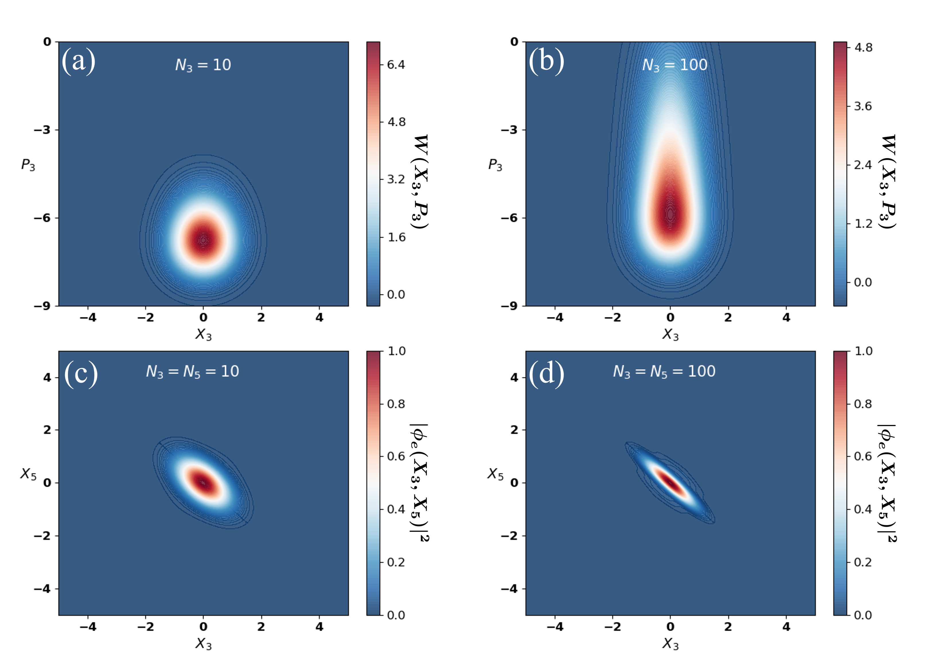
Figure 4: Examples of the harmonic states correlated to the excited state in case of resonance at all times. (a,b) Wigner functions for one of the harmonics, $n=3$, upon removing its entanglement with others, for the average number of photons $N_{3}(T)=10$ (a) and $N_{3}(T)=100$ (b). (c,d) Intensities of the entangled wavefunctions in X-quadratures for $N_{3}(T)=N_{5}(T)=10$ (c) and $N_{3}(t)=N_{5}(t)=100$ (d).

Our next example is shown in Fig.4. Here we consider exact resonance between the dressed states $|\psi_{e,g}\rangle$ at all times and perform the integration in Eq.(III) directly. For illustrative purposes we set the nonlinear response in the dressed excited state to be negligible compared to that in the dressed ground state, which is typical for a loosely bound excited state in a not-so-strong field regime, before the onset of recollision-driven harmonics. We set the resonant transition dipole matrix element $\mathbf{x}_{eg}$ to a constant. To be able to plot the resulting quantum states, we also neglect all harmonics apart from $n=3,5$.

As in the previous case of the Freeman resonances, to give an impression of the underlying structure of a single frequency mode, say $n=3$, we first artificially suppress the generation of all harmonics except for one and plot its Wigner function for $N_{3}=|\alpha_{3}(T)|^{2}=10$ and $N_{3}=|\alpha_{3}(T)|^{2}=100$, see Fig.4(a,b). We see that individual harmonics become progressively more squeezed as the number of photons in the harmonic increases. Thus, in contrast to normal expectations and standard scenarios, the quantum properties of the light state are becoming stronger as the number of photons grows. This growing squeezing is already interesting, but the overall quantum state is richer: once we include the generation of both harmonics $n=3,5$, they become entangled.

The developing quantum correlation is already apparent from the state intensity $|\phi_{e}(X_{3},X_{5})|^{2}$ shown as a function of the X-quadrature for both harmonics, which becomes both squeezed and rotated – a tell-tale sign of a correlated state. To characterize entanglement, we use both the Schmidt number and the entanglement entropy. Both are obtained from the Schmidt decomposition of $\phi_{e}(X_{3},X_{5})$ as a sum over the separable states [21, 22]: $\phi_{e}(X_{3},X_{5})=\sum_{i}\lambda_{i}\phi_{e,i}(X_{3})\phi_{e,i}(X_{5})$, where $i=1,2,3,\ldots$, $\phi_{i}(X_{3})$, $\phi_{i}(X_{5})$ represents a set of single-harmonic wavefunctions, and $\lambda_{i}>0$ are the corresponding eigenvalues of the Schmidt decomposition, normalized so that $\sum_{i}\lambda_{i}^{2}=1$. Entanglement entropy $S$ is defined then as $S=-\sum_{i}\lambda_{i}^{2}\log_{2}\lambda_{i}^{2}$, whereas the Schmidt number $D$ is defined [22] as $D=1/{\sum{\lambda_{i}^{4}}}$. If the state is separable, we have $S=0$ and $D=1$, whereas for nonseparable states $S>0$, $D>1$. Both quantities show how entangled the states are. For the generated states, these measures are shown in Figure 5, clearly demonstrating strong photon-number entanglement developed between harmonics. Importantly, the degree of entanglement and non-classicality of harmonics grows with increasing the average number of photons per harmonic, a very exciting trend.

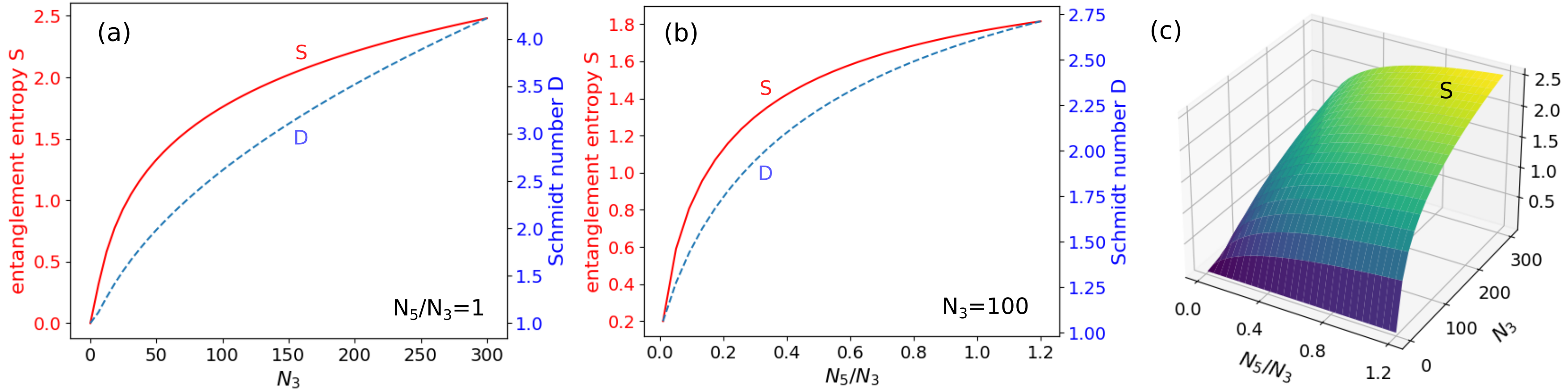
Figure 5: Entanglement entropy $S$ and the Schmidt number $D$ as functions of the average number of photons $N_{3}$ and $N_{5}$. (a) $N_{3}$ is changed, keeping constant the ratio $N_{5}/N_{3}$. (b) The ratio $N_{5}/N_{3}$ is modified, keeping $N_{3}$ constant. (c) Both $N_{3}$ and $N_{5}$ are modified (only entanglement entropy is shown).

V Conclusions and Outlook

Our work leads to several important conclusions. We find that non-trivial quantum states of harmonic light are generated as soon as quantum correlations develop between the generated light and the generating material system. A sufficient condition to developing these correlations is rather general and quite straightforward: (i) the system should undergo non-adiabatic excitations between laser dressed states and (ii) the different laser-dressed states should exhibit different non-linear responses. If this is the case, excitations of the material system into different dressed states would generate not only an entangled light-matter wavefunction, but also an entanglement between the different harmonics correlated to the excited state of the material system. Entanglement between harmonics emerges whenever the material excitation occurs at different times throughout the laser pulse.

On the one hand, a specific mechanism of resonant excitations between different laser-dressed states can be quite general and does not need to be limited to the absorption of a generated harmonic. On the other hand, resonant transitions in a strongly driven system, with large time-dependent Stark shifts, are virtually inevitable, making the process considered here rather typical.

High harmonics correlated to real excitations of matter are often ignored due to their poor phase matching properties. Indeed, excitation of loosely bound Rydberg states implies the so-called long trajectories in recollision-driven [23, 24] high harmonics. The contribution of these long trajectories to the macroscopic response is generally weak due to the large intensity-dependent phase associated with these trajectories [25, 26]. However, recent experiments and theory [27] show that this need not be the case, and that harmonics generated via excited states can even dominate the far-field spectrum. Nevertheless, to improve phase matching it might be beneficial to look at intermediate field regimes before the onset of highly non-perturbative recollision-type harmonic generation mechanisms, reducing the complexities of phase-matching large intensity-dependent harmonic phases accumulated during electron motion in the continuum.

The presence of the cavity is highly beneficial but not strictly necessary: the essential aspect is significant excitation probability. In this context, two-dimensional solid state materials, where excitons provide strong contribution to the optical response, appear an interesting candidate for generating non-classical light.

An interesting opportunity is offered by alkali atoms in a cavity. This may look like a suggestion to turn the clock back a few decades, returning to a well-studied system. However, we suggest to add a new twist: instead of driving the atomic medium with a resonant field, here we suggest to drive it with a low-frequency field, tuning the laser frequency into a multiphoton resonance with the transition between the ground and the first excited states of an alkali atom.

Control over the strengths and times of resonant excitations becomes a way of controlling the generated entanglement. We have illustrated this point by using the so-called Freeman resonances [19], which are both ubiquitous and unavoidable during intense light-matter interaction. These resonances are induced by shifting an excited state into a resonance with the ground state due to the ponderomotive shift $U_{p}=F^{2}/4\omega^{2}$ ($F$ is the field strength), associated with the wiggling energy of a loosely bound electron driven by the incident laser field. The resonance is multi-photon for the driving field and one-photon for one of the generated harmonics. Crucially, already a single resonant harmonic can trigger generation of non-trivial quantum states for all other harmonics: all it takes is for the resonant harmonic to invest its photons in material excitation, benefiting all others.

Even in the simplest case of a continuous resonance occurring throughout the whole laser pulse, which corresponds to a perturbative regime where the ponderomotive Stark shift is negligible, all harmonics correlated to the system left in the excited state are generated in non-trivial quantum states.

What is more, in contrast to normal expectations, the quantum properties of the generated harmonics become stronger as the number of photons in each harmonic grows.

We stress that the excited state is by no means obligated to efficiently generate harmonics on its own. In fact, in the cases considered here, the nonlinear components of the excited state polarization were negligible compared to those for the dressed ground state, befitting a loosely bound state in a moderate-intensity regime (before the onset of recollision-driven harmonics.)

Since Stark shifts, which control resonances in low-frequency laser fields, depend on the laser intensity, shaping the intensity envelope of the driving field shapes the quantum nature of the generated harmonic fields. Here we have only considered the case of two resonances achieved at the front and at the back of the pulse. Of course, one can control the number of resonances by shaping the laser pulse envelope in time.

At the same time, shaping the laser pulse envelope in space will generate areas in the interaction region where harmonics are generated in different entangled states. These will propagate into the far field. Thus, spatial shaping of the generating pulse and/or harmonic modes (e.g. via transverse modes of the resonant cavity) opens routes for generating highly nontrivial quantum states of light where the spatial harmonic parameters such as orbital angular momenta are also entangled.

The use of spatially structured light to shape the far-field macroscopic response, or the design of cavities to shape the transverse modes of the generated harmonics are just some examples of the additional opportunities for controlling the modes of the entangled states of high harmonics. In particular, employing a nontrivial transverse cavity mode will lead to far-field separation of harmonics correlated to the excited state and generated in nontrivial quantum states from harmonics correlated to the system left in the ground state and generated in a product of coherent states. On the one hand, this allows one to avoid the conditioning of the generated quantum states on measuring the material system in the excited state. On the other hand, such conditioning might also be possible if the excited material system is a molecule that dissociates: the measurement of light in coincidence with measuring excited atomic fragments, while extremely challenging, is not impossible.

Applications of nonclassical, massively entangled states of high harmonics can be very broad [10]. These include imaging of material properties, where nonclassical and entangled states of light provide quantum advantage [28], resulting in, for instance, enhanced absorption probability and resolution, or selectivity with respect to different quantum pathways in wave-mixing spectroscopy. Furthermore, entangled combs are known to be a resource for quantum information processing, such as quantum communication and cryptography [29]. Whereas typical combs are produced by electro-optic modulations of cavities and are limited by GHz bandwidth, the approach presented here promises to expand it to the PHz frequency range.

This discussion demonstrates truly remarkable opportunities arising when combining the fool toolkit of attosecond physics with the field of quantum optics, with exciting implications in different fields ranging from ultrafast and precision spectroscopy to quantum information science.