On the empirical spectral distribution of large wavelet random matrices based on mixed-Gaussian fractional measurements in moderately high dimensions .

Abstract

In this paper, we characterize the convergence of the (rescaled logarithmic) empirical spectral distribution of wavelet random matrices. We assume a moderately high-dimensional framework where the sample size $n$, the dimension $p(n)$ and, for a fixed integer $j$, the scale $a(n)2^{j}$ go to infinity in such a way that $\lim_{n\rightarrow\infty}p(n)\cdot a(n)/n=\lim_{n\rightarrow\infty}o(\sqrt{a(n)/n})=0$. We suppose the underlying measurement process is a random scrambling of a sample of size $n$ of a growing number $p(n)$ of fractional processes. Each of the latter processes is a fractional Brownian motion conditionally on a randomly chosen Hurst exponent. We show that the (rescaled logarithmic) empirical spectral distribution of the wavelet random matrices converges weakly, in probability, to the distribution of Hurst exponents.

1 Introduction

A wavelet is a unit $L^{2}({\mathbb{R}})$-norm function that annihilates polynomials (see (LABEL:e:N_psi)). For a fixed (octave) $j\in{\mathbb{N}}\cup\{0\}$, a wavelet random matrix is given by

$${\mathbb{R}}^{p^{2}}\ni{\boldsymbol{\boldsymbol{\mathcal{W}}}_{n}\equiv{\boldsymbol{\mathcal{W}}}}(a(n)2^{j})=\frac{1}{n_{a,j}}\sum^{n_{a,j}}_{k=1}{\mathcal{D}}(a(n)2^{j},k)\hskip 1.42262pt{\mathcal{D}}(a(n)2^{j},k)^{*}.$$ (1.1)

In (1.1), ^∗ denotes transposition, $n_{a,j}=n/a(n)2^{j}$ is the number of wavelet-domain observations for a sample size $n$. Each random vector ${\mathcal{D}}(a(n)2^{j},k)\in{\mathbb{R}}^{p}$ is the wavelet transform of a $p$-variate stochastic process $Y$ at dyadic scale $a(n)2^{j}$ and shift $k\in{\mathbb{Z}}$ (see (2.12) and (2.19) for the continuous- and discrete-time definitions, respectively). The entries of $\{{\mathcal{D}}(a(n)2^{j},k)\}_{k=1,\ldots,n_{a,j}}$ are generally correlated. A fractal is an object or phenomenon that displays the property of self-similarity, in some sense, across a range of scales (Mandelbrot mandelbrot:1982). Due to its intrinsic multiscale character and fine-tuned mathematical properties, the wavelet transform has been widely used in the study of fractals (e.g., Wornell wornell:1996, Doukhan et al. doukhan:2003, Massopust massopust:2014). In this paper, we characterize the asymptotic behavior of the (rescaled logarithmic) empirical spectral distribution of large wavelet random matrices in a moderately high-dimensional framework where the sample size $n$, the dimension $p(n)$ and the scale $a(n)2^{j}$ go to infinity. We assume measurements of the form

$$\mathbb{R}^{p}\ni Y(t)={\mathbf{P}}(n)X(t),$$ (1.2)

either in continuous or in discrete time $t$. In (1.2), the coordinates matrix ${\mathbf{P}}(n)$ is random and independent of $X(t)$. Moreover, each row of $X$ is, conditionally, an independent $H$-fractional Brownian motion, where each Hurst exponent $H$ is picked independently from a discrete probability distribution $\pi(dH)$. In the main results (Theorems 3.1 and LABEL:t:main_theorem_discrete), we show that the (rescaled logarithmic) empirical spectral distribution of ${\boldsymbol{\mathcal{W}}}(a(n)2^{j})$ converges weakly, in probability, to a known affine transformation of the distribution $\pi(dH)$ of the Hurst exponents.

In this paper, we combine two mathematical frameworks that are rarely considered jointly: $(i)$ high-dimensional probability theory; $(ii)$ fractal analysis. This is done by bringing together the study of large random matrices and scaling analysis in the wavelet domain.

Since the 1950s, the spectral behavior of large-dimensional random matrices has attracted considerable attention from the mathematical research community. For example, random matrices have proven to be prolific statistical mechanical models of Hamiltonian operators (e.g., Mehta and Gaudin mehta:gaudin:1960, Dyson dyson:1962, Ben Arous and Guionnet benarous:guionnet:1997, Soshnikov soshnikov:1999, Mehta mehta:2004, Anderson et al. anderson:guionnet:zeitouni:2010, Erdős et al. erdos:yau:yin:2012). They are also of great interest in combinatorics and numerical analysis (e.g., Baik et al. baik:deift:johansson:1999, Baik et al. baik:deift:suidan:2016, Menon and Trogdon menon:trogdon:2016), as well as in the study of integrable systems and universality (Kuijlaars and McLaughlin kuijlaars:mclaughlin:2000, Baik et al. baik:kriecherbauer:mclaughlin:miller:2007, Deift deift:2007, Tao and Vu tao:vu:2011, Borodin and Petrov borodin:petrov:2014, Deift deift:2017). In particular, the literature on random matrices under dependence has been expanding at a fast pace (e.g., Xia et al. xia:qin:bai:2013, Paul and Aue paul:aue:2014, Chakrabarty et al. chakrabarty:hazra:sarkat:2016, Che che:2017, Steland and von Sachs steland:vonsachs:2017, Wang et al. wang:aue:paul:2017, Zhang and Wu zhang:wu:2017, Erdős et al. erdos:kruger:schroder:2019, Merlevède et al. merlevede:najim:tian:2019, Bourguin et al. bourguin:diez:tudor:2021).

In turn, recall that the emergence of a fractal is typically the signature of a physical mechanism that generates scale invariance (e.g., Mandelbrot mandelbrot:1982, West et al. west:brown:enquist:1999, Zheng et al. zheng:shen:wang:li:dunphy:hasan:brinker:su:2017, He he:2018, Shen et al. shen:stoev:hsing:2022). Unlike traditional statistical mechanical systems (e.g., Reif reif:2009), a scale-invariant system does not display a characteristic scale, namely, one that dominates its statistical behavior. Instead, the behavior of the system across scales is determined by specific parameters called scaling exponents. Scale invariance manifests itself in a wide range of natural and social phenomena such as in criticality (Sornette sornette:2006), turbulence (Kolmogorov Kolmogorovturbulence), climate studies (Isotta et al. isotta:etal:2014), dendrochronology (Bai and Taqqu bai:taqqu:2018) and hydrology (Benson et al. benson:baeumer:scheffler:2006). Mathematically, it is a topic of central importance in Markovian settings (e.g., diffusion, lattice models, universality classes) as well as in non-Markovian ones (e.g., anomalous diffusion, long-range dependence, non-central limit theorems).

In a multidimensional framework, scaling behavior does not always appear along standard coordinate axes, and often involves multiple scaling relations. A ${\mathbb{R}}^{r}$-valued stochastic process $X$ is called operator self-similar (o.s.s.; Laha and Rohatgi laha:rohatgi:1981, Hudson and Mason hudson:mason:1982) if it exhibits the scaling property

$$\{X(ct)\}_{t\in{\mathbb{R}}}\stackrel{{\scriptstyle\textnormal{f.d.d.}}}{{=}}\{c^{\mathbf{H}}X(t)\}_{t\in{\mathbb{R}}},\quad c>0.$$ (1.3)

In (1.3), ${\mathbf{H}}$ is some (Hurst) matrix whose eigenvalues have real parts lying in the interval $(0,1)$ and $c^{\mathbf{H}}:=\exp\{\log(c){\mathbf{H}}\}=\sum^{\infty}_{k=0}\frac{(\log(c){\mathbf{H}})^{k}}{k!}$. A canonical model for multivariate fractional systems is operator fractional Brownian motion (ofBm), namely, a Gaussian, o.s.s., stationary-increment stochastic process (Maejima and Mason maejima:mason:1994, Mason and Xiao mason:xiao:2002, Didier and Pipiras didier:pipiras:2012). In particular, ofBm is the natural multivariate generalization of the classical fractional Brownian motion (fBm; Embrechts and Maejima embrechts:maejima:2002).

The importance of the role of multiple scaling laws in applications is now well established. For example, in econometrics, the detection of distinct scaling laws in multivariate fractional time series is indicative of the key property of cointegration – namely, the existence of meaningful and statistically useful long-run relationships among the individual series (e.g., Engle and Granger engle:granger:1987, NobelPrize.org nobelprize:2003, Hualde and Robinson hualde:robinson:2010, Shimotsu shimotsu:2012). From a different perspective, it has been shown that ignoring the presence of multiple scaling laws in statistical inference may lead to severe biases (the so-called dominance and amplitude effects – see, for instance, Abry and Didier abry:didier:2018:dim2).

In the study of scaling properties, eigenanalysis has proven to be a fecund analytic framework in a number of areas, such as in the characterization of heavy tails and correlation (e.g., Meerschaert and Scheffler meerschaert:scheffler:1999,meerschaert:scheffler:2003, Becker-Kern and Pap becker-kern:pap:2008) and in time series modeling (e.g., Phillips and Ouliaris phillips:ouliaris:1988, Li et al. li:pan:yao:2009, Zhang et al. zhang:robinson:yao:2019). In Abry and Didier abry:didier:2018:n-variate,abry:didier:2018:dim2, wavelet eigenanalysis is put forward in the construction of a general methodology for the statistical identification of the scaling (Hurst) structure of ofBm in low dimensions.

To the best of our knowledge, the behavior of the eigenvalues of large-dimensional wavelet random matrices was mathematically studied for the first time in Abry et al. abry:boniece:didier:wendt:2022,abry:boniece:didier:wendt:2023:regression. This was done in the context of a high-dimensional signal-plus-noise model where measurements display a fixed number $r$ of scaling laws, each driven by a deterministic (and unknown) Hurst exponent. In those papers, the scaling, convergence and joint fluctuations of the top $r$ eigenvalues of the associated wavelet random matrix were established and characterized.

As opposed to the “strong” approach in Abry et al. abry:boniece:didier:wendt:2022,abry:boniece:didier:wendt:2023:regression, where individual eigenvalues are tracked, in this paper we put forward a weak (or “Wigner-like”) approach. In other words, instead of assuming a fixed number of deterministic scaling laws (Hurst exponents), we suppose that, as the dimension grows, measurements display an increasing number of random scaling laws. In applications, this provides a natural model for multiparameter high-dimensional fractal systems, such as those emerging in neuroscience and fMRI imaging (Li et al. li:pluta:shahbaba:fortin:ombao:baldi:2019, Gotts et al. gotts:gilmore:martin:2020), network traffic (Abry and Didier abry:didier:2018:n-variate), climate science (Schmith et al. schmith:johansen:thejll:2012) and high-dimensional time series (Merlevède and Peligrad merlevede:peligrad:2016, Chan et al. chan:lu:yau:2017, Alshammri and Pan alshammri:pan:2021). In this context, it is of primary interest to understand the bulk behavior of the empirical spectral distribution (e.s.d.) of wavelet random matrices.

More specifically, following up on the computational study Orejola et al. orejola:didier:wendt:abry:2022, for each $n\in{\mathbb{N}}$ we assume a random vector

$$H_{1},\ldots,H_{p(n)}\in(0,1)^{p(n)}$$ (1.4)

is sampled from a discrete probability measure $\pi(dH)$ on ${\mathcal{B}}(0,1)$. Then, measurements of the form (1.2) are made, where $X$ displays independent rows and the $\ell$-th row of $X$ is, conditionally on (1.4), a fBm with Hurst parameter $H_{\ell}$ (on the recent use of this class of processes in the modeling of anomalous diffusion, see Balcerek et al. balcerek:burnecki:thapa:wylomanska:chechkin:2022). In particular, the marginal distributions of the measurement process (1.2) are random sums of mixed-Gaussian laws.

In the main results of this paper (Theorems 3.1 and LABEL:t:main_theorem_discrete), we describe the asymptotic behavior of the rescaled logarithmic e.s.d. of the wavelet random matrix

$${\boldsymbol{\mathcal{W}}}_{n}={\mathbf{W}}(a(n)2^{j})\textnormal{ or }{\boldsymbol{\mathcal{W}}}_{n}=\widetilde{{\mathbf{W}}}(a(n)2^{j}),$$ (1.5)

corresponding to continuous- and discrete-time measurements, respectively. We consider both measurement frameworks because, in the former case, exact self-similarity-type relations hold (e.g., (LABEL:e:cond_self-similarity)), which is very mathematically convenient. Once results are obtained for continuous-time measurements, then we turn to the realistic situation where measurements are made in discrete time. When taking limits, we consider a moderately high-dimensional regime where

$$\lim_{n\rightarrow\infty}\frac{p(n)\cdot a(n)}{n}=\lim_{n\rightarrow\infty}o\Big{(}\sqrt{\frac{a(n)}{n}}\Big{)}=0$$ (1.6)

(see (2.8)). Namely, the sample size $n$, the dimension $p(n)$ and the scale $a(n)2^{j}$ go to infinity in a way that $n$ grows faster than $p(n)\cdot a(n)$. Over fixed scales (i.e., when $a(n)$ is assumed constant in (1.6)), moderately high-dimensional regimes have been studied in several works. These include Bai and Yin bai:yin:1988, Jiang jiang:2008 and Wang et al. wang:aue:paul:2017 on Wigner, Jacobi and sample covariance matrices, respectively (on the use of condition (1.6) in this paper, see the discussion in Section LABEL:s:conclusion).

It is by considering the three-way limit (1.6), which includes the scaling limit $a(n)\rightarrow\infty$, that large wavelet random matrices may be used in the characterization of low-frequency behavior in a (moderately) high-dimensional framework. In fact, let $F_{{\boldsymbol{\mathcal{W}}}_{n}}(d\upsilon)$ be the rescaled logarithmic e.s.d. of ${\boldsymbol{\mathcal{W}}}_{n}$ as in (1.5) (see (3.2) and (LABEL:e:empirical_specdist_log_discrete) for the precise definition of $F_{{\boldsymbol{\mathcal{W}}}_{n}}(d\upsilon)$ for continuous- and discrete-time measurements, respectively). In Theorems 3.1 and LABEL:t:main_theorem_discrete, we show that, for any appropriate test function $g$,

$$\int_{{\mathbb{R}}}g(\upsilon)F_{{\boldsymbol{\mathcal{W}}}_{n}}(d\upsilon)\stackrel{{\scriptstyle{\mathbb{P}}}}{{\rightarrow}}\int_{{\mathbb{R}}}g(\upsilon)F_{2\mathcal{H}+1}(d\upsilon),\quad n\rightarrow\infty.$$ (1.7)

In other words, $F_{{\boldsymbol{\mathcal{W}}}_{n}}(d\upsilon)$ converges weakly, in probability, to the distribution given by the random variable $2\mathcal{H}+1$. Namely, it converges to the distribution of Hurst exponents up to a known affine transformation (see Figure 1; see also Remark LABEL:r:forces and Figure LABEL:fig:forces on a schematic representation of the “forces” acting on rescaled wavelet log-eigenvalues).

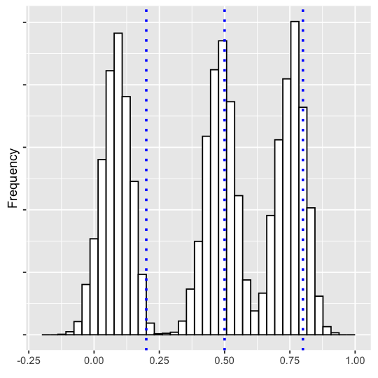
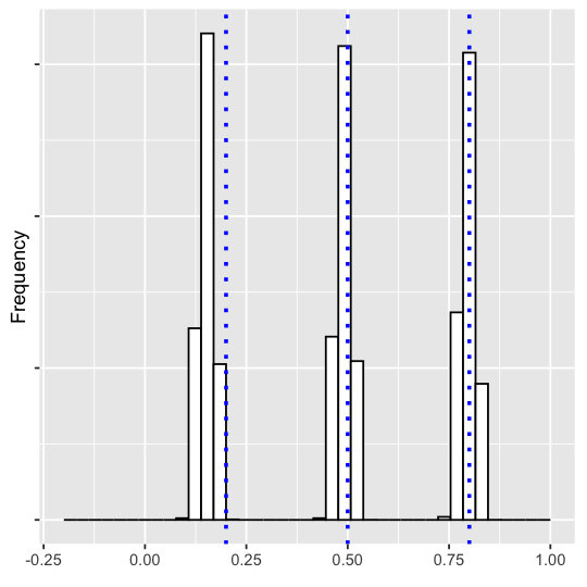
Figure 1: The distribution of the (rescaled logarithmic) wavelet e.s.d. in the three-way limit (1.6). A Monte Carlo study displays a tri-modal distribution emerging in the rescaled logarithmic wavelet e.s.d. in the three-way limit (1.6) (n.b.: after applying an affine transformation, the results are shown on the same scale as that of the distribution $\pi(dH)$). In the depicted simulation study based on $1000$ realizations, $\pi(dH)$ is a discrete uniform distribution with support $\{0.2,0.5,0.8\}$. From left to right, respectively, $(\textnormal{sample size},\textnormal{scale},\textnormal{dimension})=(2^{10},2^{4},2^{3}),(2^{15},2^{5},2^{5})$ and $(2^{18},2^{6},2^{6})$. Wavelet log-eigenvalues weighted over multiple scales were used for enhanced (“debiased”) finite-sample convergence (cf. Abry and Didier abry:didier:2018:n-variate and Abry et al. abry:boniece:didier:wendt:2022).

Note that (1.6) and (1.7) stand in sharp contrast with the traditional analysis of large random matrices. With standard sample covariance matrices, for example, one considers the ratio $\lim_{n\rightarrow\infty}p(n)/n$ and the e.s.d. often converges to a Dirac mass at a constant or to a Mar$\breve{\textnormal{c}}$enko-Pastur distribution in moderately high and in high dimensions, respectively (e.g., Chen and Pan chen:pan:2012, Bai and Silverstein bai:silverstein:2010, Tao and Vu tao:vu:2012).

In addition, statement (1.7) suggests a new form of universality that is analogous to the law of large numbers (Tao tao:2012). In other words, regardless of the underlying $\pi(dH)$, the wavelet eigenspectrum reveals the true distribution $\pi(dH)$ of the Hurst modes in the moderately high-dimensional limit (1.6).

From the standpoint of probability theory, to the best of our knowledge this paper provides the first mathematical study of the asymptotic behavior of the e.s.d. of wavelet random matrices starting from measurements containing $p(n)\rightarrow\infty$ scaling laws.

From the standpoint of fractal analysis, this paper takes a decisive step in the expansion, to the high-dimensional context, of the study of scale-invariant and non-Markovian phenomena started by Kolmogorov kolmogorov:1940 and Mandelbrot and Van Ness mandelbrot:vanness:1968, and later taken up by the likes of Flandrin flandrin:1992, Wornell and Oppenheim wornell:oppenheim:1992, Meyer et al. meyer:sellan:taqqu:1999, among many others (see Pipiras and Taqqu pipiras:taqqu:2017 and references therein).

This paper is organized as follows. In Section 2, we provide the basic wavelet framework, definitions and assumptions used throughout the paper. In Section 3, we state and establish the main results on the behavior of the rescaled logarithmic e.s.d. of wavelet random matrices in the three-way limit (1.6). The proofs of Theorems 3.1 and LABEL:t:main_theorem_discrete are written so as to provide readers with immediate access to the core ideas behind the argument, whereas the auxiliary technical results can be found in the Appendices. In Section LABEL:s:conclusion, we lay out conclusions. We also briefly discuss several open problems that this work leads to in the theory and applications of wavelet random matrices. With a view to universality claims, these include potential ways of expanding the mathematical framework of the paper.

2 Preliminaries and assumptions

2.1 Notation

Throughout the paper, we use the following notation. All with respect to the field ${\mathbb{R}}$, ${\mathcal{M}}(m_{1},m_{2},{\mathbb{R}})$ and ${\mathcal{M}}(n)={\mathcal{M}}(n,{\mathbb{R}})$ are the vector spaces, respectively, of all $m_{1}\times m_{2}$ matrices and $n\times n$ matrices, $GL(n,{\mathbb{R}})$ is the general linear group (invertible matrices), and $O(n)$ is the orthogonal group (i.e., matrices $O\in{\mathcal{M}}(n)$ such that $OO^{*}=I$). Also, ${\mathcal{S}}(n,{\mathbb{R}})$ and ${\mathcal{S}}_{\geq 0}(n,{\mathbb{R}})$ denote, respectively, the sets of $n\times n$ symmetric and symmetric positive semidefinite matrices, whereas $I=I_{n}$ denotes the $n\times n$ identity matrix. The $(n-1)$–dimensional unit sphere is represented by the symbol ${{\mathbb{S}}}^{n-1}$. For any ${\mathbf{A}}\in{\mathcal{S}}(n,{\mathbb{R}})$, the ordered eigenvalues of $\mathbf{A}$ are denoted $\lambda_{1}({\mathbf{A}})\leq\ldots\leq\lambda_{n}({\mathbf{A}})$. More generally, for ${\mathbf{M}}\in{\mathcal{M}}(n)$, the ordered singular values of ${\mathbf{M}}$ are written

$$\sigma_{1}({\mathbf{M}})\leq\ldots\leq\sigma_{n}({\mathbf{M}}).$$ (2.1)

For any ${\mathbf{A}}\in{\mathcal{M}}(n)$, $\|{\mathbf{A}}\|_{\textnormal{op}}:=\sigma_{n}({\mathbf{A}})$ is the operator norm of ${\mathbf{A}}$. The symbol $\textnormal{Haar}(O(n))$ represents the Haar probability measure on $O(n)$. The symbol $o_{{\mathbb{P}}}(1)$ denotes a random variable that vanishes in probability as $n\to\infty$. Given a collection of scalars $x_{1},\ldots,x_{n}$,

$$x_{(1)}\leq\ldots\leq x_{(n)}$$ (2.2)

denotes the associated ordered $n$-tuple.

2.2 Measurements

In regard to the underlying stochastic framework, first consider the following definition.

Definition 2.1

Let $\pi(dH)$ be a probability measure such that $\pi(0,1)=1$. The univariate stochastic process

$$X_{\mathcal{H}}=\{X_{\mathcal{H}}(t)\}_{t\in{\mathbb{R}}}$$ (2.3)

is called a random Hurst (exponent)–fractional Brownian motion (rH–fBm) when, conditionally on some value $\mathcal{H}=H$ picked from $\pi(dH)$, $X_{\mathcal{H}}$ is a standard fBm with Hurst exponent

$$H\in(0,1).$$ (2.4)

The basic properties of rH-fBm are provided in Lemma LABEL:l:properties_of_Xh(t).

So, throughout this manuscript, we make use of the following assumptions on the measurements. For expository purposes, we first state the assumptions, and then provide some interpretation. In the assumptions, ${\mathcal{T}}$ denotes either ${\mathcal{T}}={\mathbb{R}}$ or ${\mathcal{T}}=\{1,\ldots,n\}$, corresponding to the cases of continuous- or discrete-time measurements, respectively.

Assumption $(A1)$: Let $\pi(dH)$ be a distribution such that

$$\pi(0,1)=1,\quad\textnormal{supp}\ \pi(dH)=\{\breve{H}_{1},...,\breve{H}_{r}\},\quad\varpi:=\min\{\textnormal{supp}\ \pi(dH)\},$$ (2.5)

where $r\in\mathbb{N}$ and $\breve{H}_{i}\in(0,1)$ for each $i\in\{1,...,r\}$. For each $n\in\mathbb{N}$,

$$\mathds{H}_{n}=\textnormal{diag}(H_{1},\ldots,H_{p(n)})\in{\mathcal{M}}(n)$$ (2.6)

is a diagonal random matrix whose (main diagonal) entries are independently chosen from the distribution $\pi(dH)$.

Assumption $(A2)$: For each $n\in\mathbb{N}$ and given some $\mathds{H}_{n}$ as in (2.6), $p=p(n)$ independent rH–fBm sample paths are generated, each based on one of the $p$ main diagonal entries of $\mathds{H}_{n}$. In particular, when restricted to discrete time, a total of $p\times n$ entries is available. The associated $p$-variate (latent) stochastic process is denoted by $\{X(t)\}_{t\in{\mathcal{T}}}$.

Assumption $(A3)$: For $p=p(n)$ and $\{X(t)\}_{t\in{\mathcal{T}}}$ as in assumption $(A2)$, the measurements have the form

$$\mathbb{R}^{p(n)}\ni Y(t)={\mathbf{P}}(n)X(t),\quad t\in{\mathcal{T}}.$$ (2.7)

In (2.7), the so-named coordinates matrix is a random matrix ${\mathbf{P}}(n)\in GL(p(n),\mathbb{R})$ that is independent of $X(t)$.

Assumption $(A4)$: Fix $j\in{\mathbb{N}}\cup\{0\}$. The dimension $p(n)$ and the scaling factor $a(n)$ (cf. $n_{a,j}$ as in (2.15) below) satisfy the relations

$$a(n)\leq\frac{n}{2^{j}},\quad\frac{a(n)}{n}+\frac{n}{a(n)^{1+2\varpi}}\rightarrow 0,\quad p(n)<\frac{n}{a(n)2^{j}},\quad\infty\leftarrow p(n)=o\Big{(}\sqrt{\frac{n}{a(n)}}\Big{)},$$ (2.8)

as $n\to\infty$, where $\varpi$ is as in (2.5).

Assumption $(A5)$: For the random matrix ${\mathbf{P}}(n)$ as in (2.7),

$$\frac{\log\sigma_{1}(\mathbf{P}(n))}{\log a(n)}\stackrel{{\scriptstyle{\mathbb{P}}}}{{\to}}0,\quad\frac{\log\sigma_{p}(\mathbf{P}(n))}{\log a(n)}\stackrel{{\scriptstyle{\mathbb{P}}}}{{\to}}0,\quad n\rightarrow\infty.$$ (2.9)

Assumption $(A1)$ defines the distribution of Hurst exponents. Assumption $(A2)$ postulates the latent $p(n)$-variate stochastic process $X$ as a collection of independent rH-fBms. Assumption $(A3)$ describes the observed process $Y$, where the unknown random coordinates matrix ${\mathbf{P}}(n)$ determines the directions of the multiple (random) scaling relations stemming from the latent process $X$. In turn, assumption $(A4)$ controls the divergence rates among $n$, $a(n)$ and $p(n)$ in the three-way limit. In particular, it states that the scaling factor $a(n)$ and number of fractional processes, $p(n)$, must grow slower than $n$, and that the three-component ratio $\frac{p(n)a(n)}{n}$ must converge to 0 (see (1.6)). This establishes a moderately high-dimensional regime (cf. the traditional ratio $\lim_{n\rightarrow\infty}\frac{p(n)}{n}$ for sample covariance matrices). By assumption $(A5)$, the minimum and maximum singular values of ${\mathbf{P}}(n)$ neither vanish nor diverge too fast, respectively. Hence, ${\mathbf{P}}(n)$ cannot interfere too heavily on the scaling relations emanating from the latent process.

Throughout this manuscript, whenever convenient we write

$$a=a(n)\textnormal{ or }p=p(n).$$ (2.10)

Remark 2.1

Due to the many uses of the letter “$H$” throughout the paper, for the readers’ convenience we provide Table 1 to help them keep track of the notation.

notation	domain	description	defined in
$\mathbf{H}$	${\mathcal{M}}(p)$	Hurst matrix	(1.3)
$\mathds{H}_{n}$	${\mathcal{M}}(p)$	diagonal matrix whose main diagonal	(2.6)
		entries are picked from $\pi(dH)$
$\mathbb{H}_{n}$	${\mathcal{M}}(p)$	particular (deterministic) instance of $\mathds{H}_{n}$	(LABEL:e:diagonal_H_=_instance)
$\mathcal{H}$	$(0,1)$	random Hurst exponent	(2.3)
$H$	$(0,1)$	particular (deterministic) instance of $\mathcal{H}$	(2.4)
$\breve{H}$	$(0,1)$	value in $\textnormal{supp}\hskip 1.42262pt\pi(dH)$	(2.5)

Table 1: Different uses of the letter “$H$” throughout the paper.

2.3 Wavelet multiresolution analysis

Recall that a wavelet $\psi$ is a unit $L^{2}({\mathbb{R}})$-norm function that annihilates polynomials (see (LABEL:e:N_psi)). Throughout the paper, we make use of a wavelet multiresolution analysis (MRA; see Mallat mallat:1999, chapter 7). A wavelet MRA decomposes $L^{2}(\mathbb{R})$ into a sequence of approximation (low-frequency) and detail (high-frequency) subspaces $V_{j}$ and $W_{j}$, respectively, associated with different scales of analysis $2^{j}$, $j\in{\mathbb{Z}}$. In particular, given a wavelet $\psi$, there is a related scaling function $\phi\in L^{2}({\mathbb{R}})$. Appropriate rescalings and shifts of $\phi$ and $\psi$ form bases for the subspaces $V_{j}$ and $W_{j}$, respectively (see Mallat mallat:1999, Theorems 7.1 and 7.3).

In almost all mathematical statements, we make assumptions ($W1-W3$) on the underlying wavelet MRA. Such assumptions are standard in the wavelet literature and are accurately described in Section LABEL:s:assumptions_on_the_MRA. In particular, we make use of a compactly supported wavelet basis.

2.4 Wavelet random matrices: continuous time

For any $p\in{\mathbb{N}}$, suppose ${\mathcal{T}}={\mathbb{R}}$ in (2.7). Namely, assume we observe the continuous-time vector-valued stochastic process

$$\{Y(t)\}_{t\in{\mathbb{R}}}\subseteq{\mathbb{R}}^{p}.$$ (2.11)

For a wavelet function $\psi$, the wavelet transform vector of the stochastic process $Y$ is defined as the convolution

$$\mathbb{R}^{p}\ni D(2^{j},k):=2^{-j/2}\int_{\mathbb{R}}\psi(2^{-j}t-k)Y(t)dt,\quad j\in\mathbb{N}\cup\{0\},\quad k\in\mathbb{Z},$$ (2.12)

whenever such expression is meaningful. Likewise, let

$$\mathbb{R}^{p(n)}\ni D_{X}(a(n)2^{j},k):=2^{-j/2}\int_{\mathbb{R}}\psi(2^{-j}t-k)X(t)dt$$ (2.13)

be the wavelet transform of the latent process $X$ associated with $Y$. Note that, under ($A1-A5$), (2.13) is well defined in the mean squared sense by Lemma LABEL:l:D(2^j,k)_is_well_defined. Therefore, under the same conditions, (2.12) is also well defined in the mean squared sense.

So, let

$$n\in{\mathbb{N}}$$ (2.14)

be the wavelet-domain “sample size”, i.e., the number of wavelet coefficients available at scale $2^{0}=1$. Also, let $j\in{\mathbb{N}}\cup\{0\}$ and let $a(n)$ be a dyadic scaling factor. Starting from (2.12), the associated wavelet random matrices will be denoted throughout this manuscript by

$${\mathcal{S}}_{\geq 0}(p(n),{\mathbb{R}})\ni\textbf{W}(a(n)2^{j}):=\frac{1}{n_{a,j}}\sum^{n_{a,j}}_{k=1}D(a(n)2^{j},k)D(a(n)2^{j},k)^{*},\quad n_{a,j}:=\frac{n}{a(n)2^{j}}.$$ (2.15)

In (2.15), $n_{a,j}$ may be understood as the effective sample size, namely, the number of wavelet transform vectors $D(a(n)2^{j},\cdot)$ available at scale $a(n)2^{j}$. For notational convenience, we assume $n_{a,j}\in{\mathbb{N}}$ (cf. the discussion around (LABEL:e:nj=n/2^j), for the case of discrete-time measurements).

Likewise, starting from (2.13), we can define the associated wavelet random matrix

$${\mathcal{S}}_{\geq 0}(p(n),{\mathbb{R}})\ni\textbf{W}_{X}(a(n)2^{j}):=\frac{1}{n_{a,j}}\sum^{n_{a,j}}_{k=1}D_{X}(a(n)2^{j},k)D_{X}(a(n)2^{j},k)^{*}.$$ (2.16)

Note that both (2.15) and (2.16) are well defined a.s. From expressions (2.12) and (2.16), we can conveniently recast the wavelet random matrix (2.15) for the measurements (2.11) in the form

$$\textbf{W}(a(n)2^{j})={\mathbf{P}}(n)\textbf{W}_{X}(a(n)2^{j}){\mathbf{P}}(n)^{*}.$$ (2.17)

2.5 Wavelet random matrices: discrete time

Now consider the realistic situation where ${\mathcal{T}}=\{1,\ldots,n\}$ in (2.7). Namely, suppose we observe the discrete-time, vector-valued stochastic process

$$\{Y(k)\}_{k=1,\ldots,n}\subseteq{\mathbb{R}}^{p},$$ (2.18)

associated with the starting scale $2^{j}=1$ (or octave $j=0$). In particular, $n\in{\mathbb{N}}$ in (2.18) denotes the sample size (cf. (2.14)). Starting from (2.18), we suppose the wavelet transform vector $\widetilde{D}(2^{j},k)$ of the high-dimensional process $Y$ stems from Mallat’s pyramidal algorithm (Mallat mallat:1999, chapter 7). It is given by the convolution

$${\mathbb{R}}^{p}\ni\widetilde{D}(2^{j},k):=\sum_{\ell\in{\mathbb{Z}}}Y(\ell)h_{j,2^{j}k-\ell},\quad j\in{\mathbb{N}}\cup\{0\},$$ (2.19)

where we use the convention $Y(k)=0$ for $k\notin\{1,\ldots,n\}$ and the filter terms are defined by

$${\mathbb{R}}\ni h_{j,\ell}:=2^{-j/2}\int_{\mathbb{R}}\phi(t+\ell)\psi(2^{-j}t)dt,\quad\ell\in{\mathbb{Z}}.$$ (2.20)

Due to the assumed compactness of the supports of $\psi$ and of the associated scaling function $\phi$ (see condition (LABEL:e:supp_psi=compact)), only a finite number of filter terms is nonzero (Daubechies daubechies:1992). It follows that (2.19) is well defined a.s. A more detailed description of Mallat’s algorithm is provided in Section LABEL:s:Mallats_algorithm. For $n$, $j$, $a(n)$ and $n_{a,j}$ as in (2.12), the associated wavelet random matrices will be denoted throughout this manuscript by

$${\mathcal{S}}_{\geq 0}(p(n),{\mathbb{R}})\ni\widetilde{\textbf{W}}(a(n)2^{j}):=\frac{1}{n_{a,j}}\sum^{n_{a,j}}_{k=1}\widetilde{D}(a(n)2^{j},k)\widetilde{D}(a(n)2^{j},k)^{*}.$$ (2.21)

Likewise, let

$${\mathbb{R}}^{p(n)}\ni\widetilde{D}_{X}(a(n)2^{j},k):=\sum_{\ell\in{\mathbb{Z}}}X(\ell)h_{j,2^{j}k-\ell}$$ (2.22)

be the discrete-time wavelet transformation of the latent process $X$. As with (2.19), (2.22) is well defined a.s. Thus, we can naturally define the associated wavelet random matrix

$${\mathcal{S}}_{\geq 0}(p(n),{\mathbb{R}})\ni\widetilde{\textbf{W}}_{X}(a(n)2^{j}):=\frac{1}{n_{a,j}}\sum^{n_{a,j}}_{k=1}\widetilde{D}_{X}(a(n)2^{j},k)\widetilde{D}_{X}(a(n)2^{j},k)^{*}$$

$$=\frac{1}{n_{a,j}}\widetilde{D}_{X}(a(n)2^{j})\widetilde{D}_{X}(a(n)2^{j})^{*}.$$ (2.23)

In (2.23), each term $\widetilde{D}_{X}(a(n)2^{j})\in{\mathcal{M}}(p(n),n_{a,j},{\mathbb{R}})$ is a random matrix with $k$-th column given by (2.22). From expressions (2.19) and (2.23), we can conveniently recast the wavelet random matrix (2.21) for the measurements (2.18) in the form

$$\widetilde{\textbf{W}}(a(n)2^{j})={\mathbf{P}}(n)\widetilde{\textbf{W}}_{X}(a(n)2^{j}){\mathbf{P}}(n)^{*}.$$ (2.24)

3 Main results

As anticipated in the Introduction, in this section we state and prove the main results, Theorems 3.1 and LABEL:t:main_theorem_discrete, pertaining to continuous- and discrete-time measurements, respectively. For ease of understanding, the proofs of the theorems contain the bulk of the arguments. The auxiliary technical results can be found in the Appendices.

3.1 Continuous time

In this section, we consider the framework in which measurements are made in continuous time (see (2.11)). In particular, recall that, in this context, the wavelet transform is given by (2.12).

Fix $j\in{\mathbb{N}}\cup\{0\}$ as in assumption ($A4$). For notational simplicity, write

$${\mathbf{W}}_{n}={\mathbf{W}}(a(n)2^{j}).$$ (3.1)

In the first main result of this paper, we describe the asymptotic behavior of the rescaled log-eigenspectrum of the wavelet random matrix ${\mathbf{W}}_{n}$. So, to state the theorem, let

$$\lambda_{1}\big{(}{\mathbf{W}}_{n}\big{)}\leq\ldots\leq\lambda_{p(n)}\big{(}{\mathbf{W}}_{n}\big{)}$$

be the ordered eigenvalues of the wavelet random matrix ${\mathbf{W}}_{n}$. Also, let

$$F_{{\mathbf{W}}_{n}}(d\upsilon):=\frac{1}{p}\sum_{\ell=1}^{p}\delta_{\Big{\{}\frac{\log\lambda_{\ell}(\mathbf{W}_{n})}{\log a(n)}\leq\upsilon\Big{\}}}(d\upsilon)$$ (3.2)

be the empirical spectral distribution (e.s.d.) of the rescaled log-eigenvalues of ${\mathbf{W}}_{n}$. In Theorem 3.1, stated and proven next, we show that $F_{{\mathbf{W}}_{n}}(d\upsilon)$ converges weakly, in probability, to the distribution $\pi(dH)$ of the Hurst exponents up to the affine transformation $x\mapsto 2x+1$ of the latter.

Theorem 3.1

Suppose assumptions ($A1-A5$) and ($W1-W3$) hold. Then, the e.s.d. $F_{{\mathbf{W}}_{n}}$ as in (3.2) converges weakly, in probability, to $F_{2\mathcal{H}+1}$. In other words, for any $g\in C_{b}({\mathbb{R}})$ and for any $\varepsilon>0$,

$$\lim_{n\rightarrow\infty}{\mathbb{P}}\Big{(}\Big{|}\int_{{\mathbb{R}}}g(\upsilon)F_{{\boldsymbol{\mathbf{W}}}_{n}}(d\upsilon)-\int_{{\mathbb{R}}}g(\upsilon)F_{2\mathcal{H}+1}(d\upsilon)\Big{|}>\varepsilon\Big{)}=0.$$ (3.3)