Gertsenshtein-Zel^′dovich gravitational analog can enable detection of solar mass black holes in Milky way galaxy

Abstract

The Milky Way galaxy is estimated to be home to ten million to a billion stellar-mass black holes (BHs). Accurately determining this number and distribution of BH masses can provide crucial information about the processes involved in BH formation, the possibility of the existence of primordial BHs, and interpreting gravitational wave (GW) signals detected in LIGO-VIRGO-KAGRA. Sahu et al. recently confirmed one isolated stellar-mass BH in our galaxy using astrometric microlensing Sahu et al. (2022). This work proposes a novel method to identify such BHs using the gravitational analog of the Gertsenshtein-Zel^′dovich (GZ) effect. We explicitly demonstrate the generation of GWs when a kilohertz(kHz) electromagnetic (EM) pulse from a pulsar is intervened by a spherically symmetric compact object situated between the pulsar and Earth. Specifically, we show that the curvature of spacetime acts as the catalyst, akin to the magnetic field in the GZ effect. Using the covariant semi-tetrad formalism, we quantify the GW generated from the EM pulse through the Regge-Wheeler tensor and express the amplitude of the generated GW in terms of the EM energy and flux. We demonstrate how GW detectors can detect stellar-mass BHs by considering known pulsars within our galaxy. This approach has a distinct advantage in detecting stellar mass BHs at larger distances since the GW amplitude falls as $1/r$.

I Introduction

General Relativity (GR) has been an experimental triumph for over a century. Einstein’s key predictions have been verified experimentally with remarkable accuracy Will (2014a). Besides aiding in comprehending certain cosmological and astrophysical phenomena, this theory finds utility in satellite laser ranging, celestial navigation, and very long baseline interferometry (VLBI). However, several phenomena are yet to be discovered due to non-linear equations governing GR. Some phenomena, although predicted theoretically, have not been confirmed. One such phenomenon is the Gertsenshtein-Zel^′dovich (GZ) effect Gertsenshtein (1962); Pustovoit and Gertsenshtein (1962); Zel’dovich (1974); Zheng et al. (2018); Domcke and Garcia-Cely (2021).

Gertsenshtein observed that electromagnetic (EM) waves and gravitational waves (GWs) have the same propagation speeds and both are linearly related, and suggested that wave resonance should be present between them Gertsenshtein (1962); Pustovoit and Gertsenshtein (1962). Using the linearized Einstein field equations, he showed that EM waves produce GWs via wave resonance when they pass through a strong magnetic field. Similarly, GWs passing through a strong magnetic field produce EM waves Zel’dovich (1974); Kolosnitsyn and Rudenko (2015). In the quantum picture, the GZ effect can be conceptualized as the constant magnetic field facilitates the transformation of spin-1 particles (photons) to spin-2 particles (gravitons) Palessandro and Rothman (2023). To observe this effect in the laboratory requires a very high magnetic field Stephenson (2005); Aggarwal et al. (2021). Recently, it has been shown that GZ effectS explain the origin of Fast Radio Bursts Kushwaha et al. (2023).

It is natural to ask if gravity can act analogous to the magnetic field. The metric and Riemann curvature tensors play roles analogous to those of potentials and field strengths, respectively, in electromagnetism. It is important to stress that apart from the formal analogy, GR, even the linearised theory, and electromagnetism are fundamentally different Will (2014b). In spite of the difference, we explicitly show that a gravitational analog to the GZ effect exists for a static, spherically symmetric compact object. In the era of multimessenger astronomy, efforts are being made to detect the same object or event with either EM/GWs and particles (neutrinos), EM and GWs, or all three together Mészáros et al. (2019); Murase and Bartos (2019). As we show, strong gravity is observable from an entirely different perspective.

It is known that pulsars emit EM waves across the entire spectrum Ostriker and Gunn (1969); Lorimer and Kramer (2004); Condon and Ransom (2016). They are observed in radio, optical, X-ray, and $\gamma$-ray Taylor et al. (1993); Stappers et al. (2011); Johnston et al. (2021). Pulsars were first identified at 81.5 MHz, and most initial follow-ups were conducted at low frequencies (below 200 MHz) Hewish (1970). However, the preponderance of pulsar observations started in the mid-1970s at 350 MHz due to two factors Kondratiev and LOFAR Pulsar Working Group (2013); Stovall et al. (2015): Dispersion and scattering effects in the interstellar medium (ISM). According to Bates et al., pulsars typically have spectral indices in their flux densities of approximately $-1.41$ Bates et al. (2013). It is generally accepted that the radio emission (in a narrow band) is due to coherent processes, and the high-energy (x-ray and $\gamma$-ray) emission from the pulsar is due to incoherent processes, like free-free emissions Lorimer (2008). Despite numerous proposed mechanisms attempting to account for coherent radio and incoherent high-energy emissions, none have successfully explained all observed pulsar characteristics Lorimer (2008).

The magnetic dipole model is the simplest pulsar model that accounts for many of the observed properties of pulsars Goldreich and Julian (1969); Ostriker and Gunn (1969). According to this model, pulsars generate their EM radiation through the rotational energy of the neutron star Gold (1968). Consequently, the predominant EM radiation is attributed to magnetic dipole radiation, mainly at low frequencies. However, the current generation radio telescopes faces limitations in measuring radio waves below MHz. Nonetheless, the extremely low-frequency range can offer crucial insights into pulse profile evolution Lorimer and Kramer (2004), particularly given its significance at low frequencies. Although frequencies less than a few kHz cannot propagate through ISM, the frequency range between $3-6$ kHz falls for GW detection in GW detectors. The proposed mechanism provides an alternative approach to comprehending pulsars, offering an indirect means of detecting black holes (BHs) in our galaxy.

It is estimated that the Milky Way harbours around $10^{8}$ isolated BHs with an average mass of around $14M_{\odot}$, along with $9.3\times 10^{7}$ BHs engaged in binary systems, boasting an average mass of $19M_{\odot}$Olejak et al. (2020); Brown and Bethe (1994). The detection of solitary BHs poses considerable challenges using current astrophysical observational instruments. Using astrometric microlensing, identifying these BHs has become feasible Kains et al. (2018); Sahu et al. (2022). Given the prevalence of isolated stellar-mass BHs in our galaxy, the proposed mechanism presents a novel approach to detect them via GWs.

Precisely, we want to investigate low-frequency electromagnetic (EM) pulses emitted by pulsars, which, upon interaction with isolated BHs in our galaxy, generate GWs of the same frequency. As in astrometric microlensing Sahu et al. (2022), the BH is between the observer and the source. However, the key difference is that, unlike microlensing, the BH is active and converts the incoming EM waves to GWs. To quantify the generated GWs, we focus on a comoving (fictitious) observer near a static spherically symmetric spacetime and show that a test EM pulse converts to GWs by interacting with the geometry of the background spacetime. The setup is similar to Susskind’s thought experiment for EM memory Susskind (2015).

II Gravitational GZ

Consider a timelike (fictitious) observer with a worldline $\gamma$, in a locally spherically symmetric vacuum around a BH of mass ‘$m$.’ By Birkhoff’s theorem, the spacetime will be locally Schwarzschild for the observer, and by aligning the 4-velocity along the direction of the timelike Killing vector in the Schwarzschild spacetime, the observer can always be made static. As shown in Fig. 1, astrophysical phenomenon generates non-spherical EM pulse of finite duration. At a later time, the pulse passes the (fictitious) observer. Since the EM pulse travels at the speed of light, causality conditions ensure that the observer does not perceive any effect of the pulse before it reaches the worldline $\gamma$. Interactions occur during the finite duration of the pulse passage. However, being a test pulse, the components of the energy-momentum tensor are much smaller than a covariantly defined scale in the spacetime, namely the central Schwarzschild mass Goswami and Ellis (2012a).

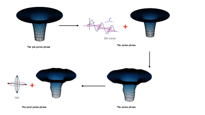
Figure 1: Gravitational analog of the GZ effect

Hence, the spacetime near the observer remains almost spherically symmetric and almost vacuum. After the pulse passes, the local spacetime returns to a vacuum state. Nevertheless, the non-sphericity persists, containing the memory of the non-spherical test pulse Jana and Shankaranarayanan (2023). This non-sphericity is subsequently radiated away through GWs, described by the traceless Regge-Wheeler tensor Clarkson and Barrett (2003a).

To rigorously and transparently analyze the outcome of this thought experiment, we divide $\gamma$ into three phases — the pre-pulse phase, the pulse phase, and the post-pulse phase. We express the field equations in terms of covariant and gauge invariant variables for each of these phases independently, up to linear order perturbations. This approach provides a comprehensive understanding of how the stress-tensor of the EM test pulse introduces geometrical variables determining linear-level non-sphericity in an open set around $\gamma$. Since the geometrical quantities of the background spherically symmetric spacetime (before the arrival of EM pulse) act as the catalyst in the generation of the GW, we term this phenomenon the gravitational analog to the GZ effect Pustovoit and Gertsenshtein (1962); Zel’dovich (1974); Gertsenshtein (1962).

To quantify the observed effect, we employ the covariant $1+1+2$ semitetrad formalism van Elst and Ellis (1996); Clarkson and Barrett (2003a); Betschart and Clarkson (2004); Hansraj et al. (2020). The observable quantities are evaluated w.r.t a comoving observer characterized by a 4-velocity $u^{a}$ satisfying $u^{a}u_{a}=-1$. Additionally, due to spherical symmetry, the spacetime features a preferred spacelike direction $n^{a}$ with $n^{a}n_{a}=1$. Thus, the 4-D spacetime metric can be decomposed as

$$g_{ab}=-u_{a}u_{b}+n_{a}n_{b}+N_{ab}\,,$$ (1)

where $N_{ab}$ is the projection tensor on the 2-D sheets orthogonal to $u^{a}$ and $n^{a}$. The directional derivative along $u^{a}$ is denoted by dot derivative ‘($\;\dot{}\;$)’ and the fully projected directional derivative along $n^{a}$ is denoted by hat derivative ‘($\;\hat{}\;$)’. The complete system is described by the geometrical variables of these two congruences (such as expansion, shear, or vorticity) along with the decomposed variables of the Weyl tensor and EM energy-momentum tensor. For details, see Refs. van Elst and Ellis (1996); Clarkson and Barrett (2003a); Betschart and Clarkson (2004); Hansraj et al. (2020) and Appendix A.

II.1 The pre-pulse phase

As discussed above and shown in Fig. 1, the causality conditions ensure that the pre-pulse phase will be spherically symmetric vacuum around an open set $\mathcal{S}$ containing $\gamma$, and hence will be locally equivalent to a part of the maximally extended Schwarzschild solution in $\mathcal{S}$. As the fictitious observer is outside the BH, we can always assume the existence of a timelike Killing vector $\xi^{a}$, for which the volume expansion ($\Theta$) and the shear scalar ($\Sigma$) vanish. By aligning the tangent of $\gamma$ to this Killing vector $\xi^{a}$ at every point in this pre-pulse phase, we can make the observer static; That is, the directional derivatives of all geometrical variables along the observer congruence (dot derivatives) vanish. The only non-zero geometrical variables in the background spacetime are Clarkson and Barrett (2003b)

$$\mathcal{D}_{0}=\{\phi,{\mathcal{A}},{\mathcal{E}}\},$$ (2)

where $\phi$ is the spatial expansion of the spacelike congruence $n^{a}$, ${\mathcal{A}}$ is the acceleration scalar for the observer, and ${\mathcal{E}}$ is the Weyl scalar extracted from the electric part of the Weyl tensor. These satisfy the following propagation (hat derivative along radial coordinate) equations

$$\hat{\phi}=-{\mathcal{E}}-\phi^{2}/2\;,\;\;\hat{\cal A}=-\left({\cal A}+\phi\right){\cal A}\;,$$ (3)

with the constraint ${\mathcal{E}}=-{\cal A}\phi$. As the spacetime is spherically symmetric, the geometry can be described by foliations of spherical 2-shells at any given instant. The Gaussian curvature of these spherical shells is

$$K=-{\mathcal{E}}+\phi^{2}/4\;.$$ (4)

From the above equations, it is clear that the electric part of the Weyl scalar is proportional to a $(3/2)th$ power of the Gaussian curvature, and the proportionality constant (which is the Schwarzschild mass ‘$m$’) produces a covariant scale in the problem. We can also define the areal radius of the spherical 2-shells $r$, such that the Gaussian curvature is $1/r^{2}$. Integrating the propagation equations in terms of this variable, we get Clarkson and Barrett (2003b)

$$K=\frac{1}{r^{2}}~{},~{}\phi=\frac{2}{r}\sqrt{F(r)}~{},~{}{\mathcal{E}}=-\frac{2m}{r^{3}}~{},~{}{\cal A}=-\frac{{\mathcal{E}}}{\phi}\,,$$ (5)

where, $F(r)\equiv 1-2m/r$. These completely specify the pre-pulse geometry.

II.2 The pulse phase

During this phase, the worldine $\gamma$ intersects the null cones of the test pulse for finite proper time. Due to the non-spherical pulse, the open sets around $\gamma$ will be non-spherical in the linear-order perturbations, which, as we show, is entirely dependent on the non-spherical energy-momentum tensor of the test pulse. In this phase, the spacetime is almost vacuum, spherical locally and, hence, almost Schwarzschild. As shown in Refs. Ellis and Goswami (2013); Goswami and Ellis (2011, 2012b), the rigidity of the vacuum spherically symmetric manifold in GR continues even in the perturbed scenario, and this almost Schwarzschild manifold will continue over the entire pulse phase. In the semitetrad formalism, the stress tensor of the test EM pulse is

$$T_{ab} = \mu u_{a}u_{b}+ph_{ab}+2{\mathcal{Q}}\,e_{(a}u_{b)}+2{\mathcal{Q}}_{(a}u_{b)}$$ (6)

$$+\Pi(e_{a}e_{b}-N_{ab}/2)+2\Pi_{(a}e_{b)}+\Pi_{ab}\;.$$

$T_{ab}$ when expressed as $E_{a},B_{a}$ does not provide much insight. For completeness, they are provided in Appendix B. In order for the pulse not to back-react with the metric, the ratio of the magnitude of each component of the above stress-tensor w.r.t the background Gaussian curvature must be less than the BH mass ($m$). This has been verified in  Refs. Ellis and Goswami (2013); Goswami and Ellis (2011, 2012b). Due to the pulse, the perturbed field equations contain both the background quantities and the first-order variables that determine the non-sphericity of the geometry. The total number of geometrical and EM pulse variables are given by $\mathcal{D}\equiv\mathcal{D}_{0}\bigcup\mathcal{D}_{1}^{\rm geom}\bigcup\mathcal{D}_{1}^{\rm EM}$, where

$$\mathcal{D}_{1}^{\rm geom} = \left\{\Theta,\hskip 0.99594pt\Omega,\hskip 0.99594pt\Sigma,\hskip 0.99594pt\mathcal{H},\hskip 0.99594pt\xi,\hskip 0.99594pt\mathcal{A}_{a},\hskip 0.99594pt\Omega_{a},\hskip 0.99594pt\Sigma_{a},\hskip 0.99594pt\alpha_{a},\hskip 0.99594pta_{a},\hskip 0.99594pt\mathcal{E}_{a},\hskip 0.99594pt\mathcal{H}_{a},\right.$$ (7)

$$\left.\hskip 0.99594pt\Sigma_{ab},\hskip 0.99594pt\zeta_{ab},\hskip 0.99594pt\mathcal{E}_{ab},\hskip 0.99594pt\mathcal{H}_{ab}\right\}$$

$$\mathcal{D}_{1}^{\rm EM} = \left\{\mu,\hskip 0.99594ptp,\hskip 0.99594pt{\mathcal{Q}},\hskip 0.99594pt\Pi,\hskip 0.99594pt{\mathcal{Q}}_{a},\hskip 0.99594pt\Pi_{a},\hskip 0.99594pt\Pi_{ab}\right\}.$$ (8)

Physical observables in GR must be gauge-invariant van Elst and Ellis (1996). We need to identify the gauge-invariant variables from the above set to compare the derived quantities with observations. Pulse introduces variations in $u^{a}$ and $n^{a}$ along spacelike and timelike directions, rendering the variables in the set $\mathcal{D}_{0}$ non-gauge-invariant. As per the Stewart-Walker lemma, the quantities that vanish in the background spacetime are automatically gauge-invariant Stewart and Walker (1974); Ellis and Bruni (1989). For complete gauge invariance, we replace these variables with the following three Betschart and Clarkson (2004); Nzioki et al. (2016)

$$\mathcal{D}_{1}^{\rm GI}=\left\{W_{a}=\delta_{a}{\mathcal{E}},Y_{a}=\delta_{a}\phi,Z_{a}=\delta_{a}{\cal A}\right\}.$$ (9)

Hence, the complete set of first-order variables $\mathcal{D}_{1}^{\rm GI}\bigcup\mathcal{D}_{1}^{\rm geom}\bigcup\mathcal{D}_{1}^{\rm EM}$, determine the perturbed spacetime in a covariant and gauge-invariant way. For these variables, linearized evolution and propagation equations can be written as follows

$$\mathcal{L}^{(\rho)}\mathcal{D}^{\rm GI}=\mathcal{D}^{\rm geom}+f(\mathcal{D}^{\rm EM})\,,$$ (10)

where, $\mathcal{L}^{(\rho)}$ represents evolution, propagation, or projected covariant derivatives on $2-$space. For details, see Appendix C. One key feature of these equations is that the stress-tensor of the EM field (at the instant when the pulse reaches the worldline $\gamma$) sources these linearized equations. Since the $\mathcal{D}^{\rm geom}$ variables vanish before the pulse arrives, the non-trivial initial data that generated these gauge-invariant variables in the pulse phase are completely supplied by the EM pulse.

II.3 The post pulse phase

As the pulse leaves the fictitious observer, the open set $\mathcal{S}$ containing the $\gamma$ post-pulse will revert to its vacuum state. However, the non-sphericity will persist. The initial data that evolves the non-sphericity variables in the post-pulse phase are those that Cauchy evolved from the EM pulse initial data of the test pulse in the pulse phase. This clearly shows how the local inherent Killing symmetry of the spacetime becomes altered as the test pulse passes the open set $\mathcal{S}$ containing $\gamma$. Physically, we can view this process as a perturbed black hole relaxing to a stationary black hole by emitting QNMs Chandrasekhar (1992).

To see transparently how the non-sphericity of the open set is radiated away via GWs, we construct the following dimensionless, covariant, gauge invariant, frame invariant, transverse trace-free tensor $M_{\{ab\}}$ Betschart and Clarkson (2004); Nzioki et al. (2016)

$$M_{ab}=\phi\,r^{2}\,\zeta_{ab}/2-r^{2}\,{\mathcal{E}}^{-1}\,\delta_{\{a}W_{b\}}/3\;.$$ (11)

$\zeta_{ab}$ represents distortion of the 2-D sheet and quantifies GW amplitude in free space. $M_{ab}$ is the Regge-Wheeler tensor and obeys the following closed wave equation for odd and even parity cases

$$\ddot{M}_{\{ab\}}-\hat{\hat{M}}_{\{ab\}}-{\cal A}\,{\hat{M}}_{\{ab\}}+[\phi^{2}+{\mathcal{E}}]M_{ab}-\delta^{2}M_{ab}=0~{}.$$ (12)

Interestingly, the tensor $M_{ab}$ gives a measure of sheet deformation via the electric part of the Weyl scalar and the deformation tensor related to the preferred spacelike direction Clarkson and Barrett (2003a); Clarkson et al. (2004). In the pre-pulse phase $M_{ab}=0$, while $M_{ab}\neq 0$ in the post-pulse phase. Thus, the Regge-Wheeler tensor contains the memory of the EM pulse Jana and Shankaranarayanan (2023). Thus, the background quantities $(\phi,{\mathcal{E}})$ act as the catalyst, akin to the magnetic field in the GZ effect.

To investigate the nature of the GWs and their dependence on the EM pulse stress tensor, we decompose the geometrical variables as an infinite sum of components relative to a basis of harmonic functions. This allows us to replace angular derivatives appearing in the equations with a harmonic coefficient. Following Ref. Clarkson and Barrett (2003b), we introduce a set of dimensionless spherical harmonics $Q=Q^{(\ell,m)}$ ($m=-\ell,\cdots,\ell$), defined in the background, as eigenfunctions of the spherical Laplacian operator: $\delta^{2}Q=-[\ell(\ell+1)/r^{2}]\,Q$, $\hat{Q}=\dot{Q}=0$. Expanding the first-order scalar ${\Psi}$ in terms of harmonic functions

$${\Psi}=\sum_{\ell=0}^{\infty}\sum_{m=-\ell}^{m=\ell}{\Psi}_{\mathsf{S}}^{(\ell,m)}Q^{(\ell,m)}={\Psi}_{\mathsf{S}}\,Q,$$ (13)

where the sum over $\ell$ and $m$ is implicit in the last equality. The replacements that must be made for scalars when expanding the equations in spherical harmonics are

$$\!\!{\Psi}={\Psi}_{\mathsf{S}}\,Q~{},\delta_{a}{\Psi}=r^{-1}{\Psi}_{\mathsf{S}}\,Q_{a}~{},\varepsilon_{ab}\delta^{b}{\Psi}=r^{-1}{\Psi}_{\mathsf{S}}\,\bar{Q}_{a}\,,$$ (14)

where the sums over $\ell$ and $m$ are implicit and $\bar{Q}_{a}$ is the odd parity vector harmonics. Note that the moment the EM pulse arrives, $\dot{W}_{a}$ is non-zero (even if other non-spherical $\mathcal{D}^{\rm geom}$ quantities are zero).

$$\dot{W}_{a}=-\frac{1}{2}\phi\left(\delta_{a}{\mathcal{Q}}\right)-\frac{2}{3}\delta_{a}\dot{\mu}$$ (15)

Since the background space-time is Schwarzschild, we set $u^{a}\equiv(\,1/\sqrt{F(r)},\,0,\,0,\,0)$. Integrating the above equation w.r.t the Schwarzschild coordinate time $t$, we get

$$W_{a}=-\frac{F(r)^{\frac{1}{2}}}{2}\phi\left(\delta_{a}\int dt\,{\mathcal{Q}}\right)-\frac{2}{3}\delta_{a}\mu+C_{1}(\theta,\,\phi).$$ (16)

Rewriting in terms of spherical and time harmonics as

$$\left(\int dt\,{{\mathcal{Q}}}\right)=T^{(\omega)}{{\mathcal{Q}}}_{\mathsf{S}}\,Q,\;\;\mu=T^{(\omega)}{\mu}_{\mathsf{S}}\,Q,$$ (17)

and decomposing $M_{ab}=T^{(\omega^{{}^{\prime}})}{M}_{\mathsf{T}}\,Q_{ab}$ (where $Q_{ab}=\delta_{\{a}\delta_{b\}}\,Qr^{2}$ is the electric parity tensor spherical harmonics, $\omega$ is the frequency of the incoming EM pulse and $\omega^{{}^{\prime}}$ represents the frequency of the generated GW), Eq. (11) becomes

$$T^{(\omega^{{}^{\prime}})}{M}_{\mathsf{T}}\,Q_{ab} = (r^{2}/6)F(r)^{\frac{1}{2}}r^{2}\,\phi\,{\mathcal{E}}^{-1}\,\delta_{\{a}\delta_{b\}}T^{(\omega)}{{\mathcal{Q}}}_{\mathsf{S}}\,Q$$ (18)

$$+(2r^{2}/9)\,{\mathcal{E}}^{-1}\,\delta_{\{a}\delta_{b\}}T^{(\omega)}{\mu}_{\mathsf{S}}\,Q,$$

At resonance, $\omega=\omega^{{}^{\prime}}$, the amplitudes of EM and GWs are related by

$${M}_{\mathsf{T}}\,=-\frac{r^{2}}{6m}\left(1-\frac{2m}{r}\right){{\mathcal{Q}}}_{\mathsf{S}}-\frac{1}{9}\,\frac{r^{3}}{m}{\mu}_{S},$$ (19)

where ${\mathcal{Q}}_{\mathsf{S}}$ is the time integral of the amplitude of the EM Poynting vector component ${\mathcal{Q}}$ and $\mu_{\mathsf{S}}$ is the EM energy density and can be related to the Luminosity $({\cal L}_{\rm EM})$ via the relation ${\cal L}_{\rm EM}\,\Delta t$ where $\Delta t$ is the pulse duration.

This is the key result of this work, regarding which we want to discuss the following points: Firstly, the above relation is only applicable in the close vicinity of the fictitious observer $\gamma$, while interacting with the EM pulse in the pulse phase. At the moment of the EM pulse arrives $\dot{\zeta}_{ab}=0$, while another first order variable $\Sigma_{ab}$ sources $\ddot{\zeta}_{ab}$. Hence when calculating the Regge Wheeler tensor we can safely neglect the $\zeta_{ab}$ term.

Secondly, the outgoing GW amplitude depends on the Poynting vector and energy density Jana and Shankaranarayanan (2023). In other words, the contribution to the QNMs arises from the EM memory. As we show, this can be observable in the next generation GW experiments. Thirdly, like the canonical GZ effect, the amplitude is maximum at the resonance and is suppressed away from the resonance. Thus, detecting such a GW signal provides information on the incoming EM wave. If the incoming EM waves are coherent and monochromatic, this mechanism can provide key properties of various astrophysical processes that are beyond the reach of telescopes in the EM band. Lastly, ${M}_{\mathsf{T}}$ derived above is for the static observer w.r.t the BH. To compare with the observations, we need to transform the above quantity to the static (detector) frame. Since, ${M}_{\mathsf{T}}$ is gauge and frame invariant Clarkson and Barrett (2003a), in asymptotically flat spacetime (${\mathcal{E}}\sim 1/r^{3},\phi\sim 1/r$), we have $M_{ab}\sim r\zeta_{ab}$. $\zeta_{ab}$ is related to plane GW in Minkowski space-time via the relation: $\zeta_{ab}\sim(1/2)\partial_{z}h_{ab}^{\rm TT}$ Clarkson et al. (2004).

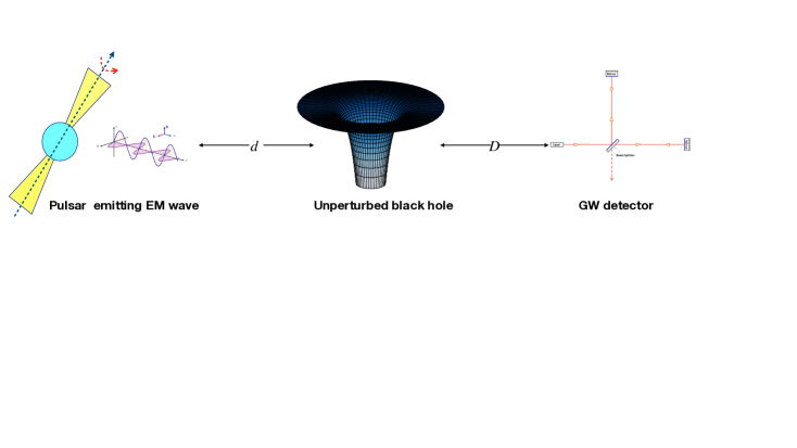
Figure 2: Schematic figure showing the location of Pulsar, spherically symmetric compact object, and the earth or space-based detector.

III Observational implications and conclusions

We now discuss the implications of our results for stellar mass BH observations in our galaxy. As mentioned earlier, pulsars emit radiation across the entire electromagnetic spectrum, and the magnetic dipole model illustrates the origin of pulsar emission from the rotational kinetic energy of a neutron star Condon and Ransom (2016). While pulsars are stable to a precision that rivals atomic clocks, many pulsars show sudden spin-up events, referred to as glitches Haskell and Melatos (2015); Zhou et al. (2022). The pulse profile associated with these glitches (in Vega and Crab) suggests an internal origin. However, no mechanism can explain these glitches Haskell and Melatos (2015); Zhou et al. (2022).

As shown in Fig. 2, consider a BH intervening pulsar and Earth. Let the distance between the pulsar and the BH be $d$, and the distance between the BH and the Earth by $D$. A typical pulsar in our galaxy is at a kpc distance from the Earth Manchester et al. (2005); Lopez-Coto et al. (2022), hence we set $d\sim D\sim kpc$. The magnetic dipole model Condon and Ransom (2016) predicts pulsars with intrinsic luminosity ${\cal L}_{\rm EM}\sim{\Omega_{0}^{4}}\,10^{38}~{}{\rm erg}/s$ where $\Omega_{0}$ is the dimensionless frequency scaled w.r.t $30~{}{\rm Hz}$, i. e., $\Omega_{0}=\Omega_{e}/30$. [Depending on the pulsar, we have $10^{3}\leq\Omega_{0}\leq 1$ Manchester et al. (2005); Lorimer and Kramer (2004).] Since the Poynting vector remains the same at the source and the detector, the flux emanating from the pulsar will be the same as the flux received by the fictitious observer near the solar mass BH.

Substituting the above Luminosity, $\Delta t\sim 1\,s$ and $r\sim 10^{5}{\rm cm}$ (Schwarzschild radius) in Eq. (19), we get

$$M_{\rm T}\sim{\Omega_{0}^{4}}\,10^{-2}\,.$$ (20)

This is the GW amplitude measured by the fictitious observer near the BH. Details extended in the Appendix D. As mentioned above, the GW amplitude measured by the GW detector on Earth is given by $\zeta_{ab}$, hence, $h_{\rm T}\propto M_{\rm T}/D$ Creighton and Anderson (2011). Setting $D\sim{\rm kpc}$, we have $h_{\rm T}\sim\Omega_{0}^{4}\,10^{-23}$. This amplitude is well in line with the expected sensitivity of Einstein Telescope and Cosmic Explorer in the frequency range $3-6~{}$kHz Hild et al. (2011); Maggiore et al. (2020); Evans et al. (2021); Srivastava et al. (2022).

To conclude, the gravitational analog of the GZ effect enables the detection of solar mass black holes in the Milky Way galaxy. Though our analysis is for a Solar-mass BH, the analysis is applicable for any non-rotating compact object, including some exotic compact objects Cardoso and Pani (2019); Völkel (2020). This approach has one distinct advantage over the astrometric microlensing Sahu et al. (2022) — it can probe BHs at larger distance. In the case of microlensing, the detection is through the measurement of photon energy, which falls off as $1/D^{2}$. However, our approach uses GW amplitude, which falls as $1/D$. Hence, it can be a definite probe for detecting stellar mass BHs at further distances. This approach introduces novel possibilities for identifying and studying stellar-mass BHs through their interactions with EM pulses from pulsars.

Appendix A Semiterad covariant formalism

In this section, we briefly recapitulate the semi-tetrad formalisms developed in Ellis and van Elst (1999); Clarkson and Barrett (2003b), which enables us to study the problem geometrically. The key point of these semi-tetrad decompositions is that they are local decompositions defined on any open set $\mathcal{S}$. In the first step of this decomposition, the properties of spacetime are studied with respect to a real or fictitious observer whose velocity is along the tangent of a timelike congruence. Thereafter, if the spacetime has certain symmetries like local rotational symmetry, a preferred spatial direction exists. The spacetime is then further decomposed using this preferred spatial congruence. The field equations are then recast in terms of the geometrical variables related to these congruences and the curvature tensor of the spacetime (suitably decomposed using the congruences).

A.1 Semitetrad 1+3 formalism

$1+3$ covariant formalism is a well-known formalism widely used to study relativistic cosmology in the frame of different models of general relativity(GR) and cosmology. The spacetime is locally sliced into the timelike direction $u^{a}\equiv dx^{a}/d\tau$ and spacelike hypersurface, which is orthogonal to $u^{a}$. Here, $\tau$ is the affine parameter. In the 1+3 formalism Ellis and van Elst (1999), the timelike unit vector ${u^{a}}$ ${\left(u^{a}\hskip 0.99594ptu_{a}=-1\right)}$ is used to split the spacetime locally in the form ${\mathcal{R}\otimes\mathcal{V}}$, where ${\mathcal{R}}$ is the timeline along ${u^{a}}$ and ${\mathcal{V}}$ is the 3-space perpendicular to ${u^{a}}$. Thus, the metric becomes

$$g_{ab}=-u_{a}\hskip 0.99594ptu_{b}+h_{ab},$$ (21)

where ${h_{ab}}$ is the projection tensor used to project any vector or tensor on 3-space perpendicular to $u^{a}$. $h_{ab}$ becomes metric of the $3-$space iff there is no twist or vorticity in the $3-$space. The covariant time derivative along the observers’ worldlines, denoted by ‘${\hskip 0.99594pt\hskip 0.99594pt{}^{\cdot}\hskip 0.99594pt\hskip 0.99594pt}$’, is defined using the vector ${u^{a}}$, as

$$\dot{Z}^{a...b}{}_{c...d}=u^{e}\hskip 0.99594pt\nabla_{e}\hskip 0.99594ptZ^{a...b}{}_{c...d},$$ (22)

for any tensor ${Z^{a...b}{}_{c...d}}$. The fully orthogonally projected covariant spatial derivative, denoted by ‘ ${D}$ ’, is defined using the spatial projection tensor ${h_{ab}}$, as

$$D_{e}\hskip 0.99594ptZ^{a...b}{}_{c...d}=h^{r}{}_{e}\hskip 0.99594pth^{p}{}_{c}\hskip 0.99594pt...\hskip 0.99594pth^{q}{}_{d}\hskip 0.99594pth^{a}{}_{f}\hskip 0.99594pt...\hskip 0.99594pth^{b}{}_{g}\hskip 0.99594pt\nabla_{r}\hskip 0.99594ptZ^{f...g}{}_{p...q},$$ (23)

with total projection on all the free indices. The covariant derivative of the 4-velocity vector ${u^{a}}$ is decomposed irreducibly as follows

$$\nabla_{a}\hskip 0.99594ptu_{b} = -u_{a}\hskip 0.99594ptA_{b}+\frac{1}{3}h_{ab}\hskip 0.99594pt\Theta+\sigma_{ab}+\epsilon_{abc}\hskip 0.99594pt\omega^{c},$$ (24)

where ${A_{b}}$ is the acceleration, ${\Theta}$ is the expansion of ${u_{a}}$, ${\sigma_{ab}}$ is the shear tensor, ${\omega^{a}}$ is the vorticity vector representing rotation and ${\epsilon_{abc}}$ is the effective volume element in the rest space of the comoving observer. The vorticity vector $\omega^{q}$ is related to vorticity tensor $\omega^{ab}$ as: $\omega^{a}\equiv(1/2)\,\epsilon^{abc}\,\omega_{bc}$.

Furthermore, the energy-momentum tensor of matter or fields present in the spacetime, decomposed relative to ${u^{a}}$, is given by

$$T_{ab} = \mu\hskip 0.99594ptu_{a}\hskip 0.99594ptu_{b}+p\hskip 0.99594pth_{ab}+q_{a}\hskip 0.99594ptu_{b}+u_{a}\hskip 0.99594ptq_{b}+\pi_{ab},$$ (25)

where ${\mu}$ is the effective energy density, ${p}$ is the isotropic pressure, ${q_{a}}$ is the 3-vector defining the heat flux and ${\pi_{ab}}$ is the anisotropic stress. Angle brackets denote orthogonal projections of vectors onto the three space as well as the projected, symmetric and trace-free (PSTF) part of tensors.

$$v_{<a>} = h^{b}{}_{a}\hskip 0.99594pt\dot{V}_{b},$$ (26)

$$Z_{<ab>} = \left(h^{c}{}_{(a}\hskip 0.99594pth^{d}{}_{b)}-\frac{1}{3}h_{ab}\hskip 0.99594pth^{cd}\right)\hskip 0.99594ptZ_{cd}.$$ (27)

The Weyl quantities are decomposed as

$$E_{ab} = C_{abcd}\hskip 0.99594ptu^{c}\hskip 0.99594ptu^{d}=E_{<ab>},$$ (28)

$$H_{ab} = \frac{1}{2}\varepsilon_{ade}\hskip 0.99594ptC^{de}{}_{bc}\hskip 0.99594ptu^{c}=H_{<ab>}.$$ (29)

A.2 Semitetrad 1+1+2 formalism

In the 1+1+2 formalism Clarkson and Barrett (2003b), the 3-space ${\mathcal{V}}$ is now further split by introducing the unit vector ${e^{a}}$ orthogonal to ${u^{a}}$ ${\left(e^{a}\hskip 0.99594pte_{a}=1,u^{a}\hskip 0.99594pte_{a}=0\right)}$. The $3-$space now has two parts—one is the spacelike direction $e^{a}$, and the second is the $2-$space orthogonal to $e^{a}$ as well as $u^{a}$, which we refer to as the $2-sheets$. The 1+1+2 covariantly decomposed spacetime is given by

$$g_{ab}=-u_{a}\hskip 0.99594ptu_{b}+e_{a}\hskip 0.99594pte_{b}+N_{ab},$$ (31)

where ${N_{ab}}$ ${\left(e^{a}\hskip 0.99594ptN_{ab}=0=u^{a}\hskip 0.99594ptN_{ab},N^{a}{}_{a}=2\right)}$ projects vectors onto 2-spaces called ‘2-sheets’ , orthogonal to ${u^{a}}$ and ${e^{a}}$. We introduce two new derivatives for any tensor ${\phi_{a...b}{}^{c...d}}$:

$$\hat{\phi}_{a...b}{}^{c...d} \equiv e^{f}\hskip 0.99594ptD_{f}\hskip 0.99594pt\phi_{a...b}{}^{c...d},$$ (32)

$$\delta_{f}\phi_{a...b}{}^{c...d} \equiv N_{f}{}^{j}N_{a}{}^{l}...N_{b}{}^{g}N_{h}{}^{c}...N_{i}{}^{d}D_{j}\phi_{l...g}{}^{h...i}.$$ (33)

The 1+3 kinematical and dynamical quantities and anisotropic fluid variables are split irreducibly as

$$A^{a} = \mathcal{A}\hskip 0.99594pte^{a}+\mathcal{A}^{a},$$ (34)

$$\omega^{a} = \Omega\hskip 0.99594pte^{a}+\Omega^{a},$$ (35)

$$\sigma_{ab} = \Sigma\left(e_{a}\hskip 0.99594pte_{b}-\frac{1}{2}\hskip 0.99594ptN_{ab}\right)+2\hskip 0.99594pt\Sigma_{(a}\hskip 0.99594pte_{b)}+\Sigma_{ab},$$ (36)

$$q_{a} = {\mathcal{Q}}\hskip 0.99594pte_{a}+{\mathcal{Q}}_{a},$$ (37)

$$\pi_{ab} = \Pi\left(e_{a}\hskip 0.99594pte_{b}-\frac{1}{2}\hskip 0.99594ptN_{ab}\right)+2\hskip 0.99594pt\Pi_{(a}\hskip 0.99594pte_{b)}+\Pi_{ab},$$ (38)

$$E_{ab} = \mathcal{E}\left(e_{a}\hskip 0.99594pte_{b}-\frac{1}{2}\hskip 0.99594ptN_{ab}\right)+2\hskip 0.99594pt\mathcal{E}_{(a}\hskip 0.99594pte_{b)}+\mathcal{E}_{ab},$$ (39)

$$H_{ab} = \mathcal{H}\left(e_{a}\hskip 0.99594pte_{b}-\frac{1}{2}\hskip 0.99594ptN_{ab}\right)+2\hskip 0.99594pt\mathcal{H}_{(a}\hskip 0.99594pte_{b)}+\mathcal{H}_{ab}\,.$$ (40)

The fully projected 3-derivative of ${e^{a}}$ is given by

$$D_{a}\hskip 0.99594pte_{b} = e_{a}\hskip 0.99594pta_{b}+\frac{1}{2}\hskip 0.99594pt\phi\hskip 0.99594ptN_{ab}+\xi\hskip 0.99594pt\varepsilon_{ab}+\zeta_{ab},$$ (41)

where traveling along ${e^{a}}$, ${a_{a}}$ is the sheet acceleration, ${\phi}$ is the sheet expansion, ${\xi}$ is the vorticity of ${e^{a}}$ (the twisting of the sheet) and ${\zeta_{ab}}$ is the shear of ${e^{a}}$ (the distortion of the sheet).

The 1+1+2 split of the full covariant derivatives of ${u^{a}}$ and ${e^{a}}$ are as follows

$$\nabla_{a}\hskip 0.99594ptu_{b} = -u_{a}\left(\mathcal{A}\hskip 0.99594pte_{b}+\mathcal{A}_{b}\right)+e_{a}\hskip 0.99594pte_{b}\left(\frac{1}{3}\hskip 0.99594pt\Theta+\Sigma\right)+e_{a}\left(\Sigma_{b}+\varepsilon_{bc}\hskip 0.99594pt\Omega^{c}\right)+\left(\Sigma_{a}-\varepsilon_{ac}\hskip 0.99594pt\Omega^{c}\right)e_{b}$$ (42)

$$+N_{ab}\left(\frac{1}{3}\hskip 0.99594pt\Theta-\frac{1}{2}\hskip 0.99594pt\Sigma\right)+\Omega\hskip 0.99594pt\varepsilon_{ab}+\Sigma_{ab},$$

$$\nabla_{a}\hskip 0.99594pte_{b} = -\mathcal{A}\hskip 0.99594ptu_{a}\hskip 0.99594ptu_{b}-u_{a}\hskip 0.99594pt\alpha_{b}+\left(\frac{1}{3}\hskip 0.99594pt\Theta+\Sigma\right)e_{a}\hskip 0.99594ptu_{b}+\left(\Sigma_{a}-\varepsilon_{ac}\hskip 0.99594pt\Omega^{c}\right)u_{b}+e_{a}\hskip 0.99594pta_{b}$$ (43)

$$+\frac{1}{2}\hskip 0.99594pt\phi\hskip 0.99594ptN_{ab}+\xi\hskip 0.99594pt\varepsilon_{ab}+\zeta_{ab}.$$

We can now immediately see that the Ricci identities and the doubly contracted Bianchi identities, which specify the evolution of the complete system, can now be written as the time evolution and spatial propagation and spatial constraints of an irreducible set of geometrical and electromagnetic (EM) variables. The irreducible set of geometric variables

$$\mathcal{D}_{geom}=\{\Theta,\hskip 0.99594pt\mathcal{A},\hskip 0.99594pt\Omega,\hskip 0.99594pt\Sigma,\hskip 0.99594pt\mathcal{E},\hskip 0.99594pt\mathcal{H},\hskip 0.99594pt\phi,\hskip 0.99594pt\xi,\hskip 0.99594pt\mathcal{A}_{a},\hskip 0.99594pt\Omega_{a},\hskip 0.99594pt\Sigma_{a},\hskip 0.99594pt\alpha_{a},\hskip 0.99594pta_{a},\hskip 0.99594pt\mathcal{E}_{a},\hskip 0.99594pt\mathcal{H}_{a},\hskip 0.99594pt\Sigma_{ab},\hskip 0.99594pt\zeta_{ab},\hskip 0.99594pt\mathcal{E}_{ab},\hskip 0.99594pt\mathcal{H}_{ab}\}$$ (44)

together with the irreducible set of EM variables

$$\mathcal{D}_{\rm EM} = \left\{\mu,\hskip 0.99594ptp,\hskip 0.99594pt{\mathcal{Q}},\hskip 0.99594pt\Pi,\hskip 0.99594pt{\mathcal{Q}}_{a},\hskip 0.99594pt\Pi_{a},\hskip 0.99594pt\Pi_{ab}\right\},$$ (45)

make up the key variables in the 1+1+2 formalism.

Appendix B The energy momentum tensor of the EM test pulse

The test pulse contains the electromagnetic field that perturbs the background spacetime. By virtue of the semitetrad 1+1+2 splitting, the electric and magnetic field vectors can be written in the following way:

$$E^{a} = \mathscr{E}e^{a}+\mathscr{E}^{a}\;,$$ (46)

$$B^{a} = \mathscr{B}e^{a}+\mathscr{B}^{a}\;,$$ (47)

where $\mathscr{E}$ and $\mathscr{B}$ are scalars and $\mathscr{E}^{a}$ and $\mathscr{B}^{a}$ are projected 2-vectors on the 2-shells that break the sphericity of these shells. The energy-momentum tensor $T_{ab}$ of the field can then be split into a scalar, 2-vector, PSTF 2-tensor parts as

$$T_{ab}=\mu u_{a}u_{b}+ph_{ab}+2{\mathcal{Q}}\,e_{(a}u_{b)}+2{\mathcal{Q}}_{(a}u_{b)}+\Pi(e_{a}e_{b}-\frac{1}{2}N_{ab})+2\Pi_{(a}e_{b)}+\Pi_{ab}\;,$$ (48)

where,

$$\mu = \frac{1}{2}(\mathscr{E}^{2}+\mathscr{B}^{2}+\mathscr{E}^{a}\mathscr{E}_{a}+\mathscr{B}^{a}\mathscr{B}_{a})\;$$ (49)

$$p = \frac{1}{6}(\mathscr{E}^{2}+\mathscr{B}^{2}+\mathscr{E}^{a}\mathscr{E}_{a}+\mathscr{B}^{a}\mathscr{B}_{a})\;$$ (50)

$${\mathcal{Q}} = \varepsilon_{ab}\,\mathscr{E}^{b}\mathscr{B}^{c}\;$$ (51)

$${\mathcal{Q}}_{a} = \varepsilon_{ac}(\mathscr{B}\mathscr{E}^{c}-\mathscr{E}\mathscr{B}^{c})\;$$ (52)

$$\Pi = \frac{1}{3}\left[-2(\mathscr{E}^{2}+\mathscr{B}^{2})+(\mathscr{E}^{a}\mathscr{E}_{a}+\mathscr{B}^{a}\mathscr{B}_{a})\right]\;$$ (53)

$$\Pi_{a} = -\left(\mathscr{E}\mathscr{E}_{a}+\mathscr{B}\mathscr{B}_{a}\right)\;$$ (54)

$$\Pi_{ab} = \frac{1}{2}(\mathscr{E}^{c}\mathscr{E}_{c}+\mathscr{B}^{c}\mathscr{B}_{c})N_{ab}-(\mathscr{E}_{a}\mathscr{E}_{b}+\mathscr{B}_{a}\mathscr{B}_{b})\;.$$ (55)

For the pulse not to back-react on the metric, the ratio of the magnitude of each component of the above stress-tensor w.r.t the background Gaussian curvature must be less than the BH mass ($m$). This has been verified in  Refs. Ellis and Goswami (2013); Goswami and Ellis (2011, 2012b). The above energy-momentum tensor must follow the conservation equations up to the first-order perturbations on the background Schwarzschild manifold of the pre-pulse phase, which are given as

$$\dot{\mu}+\hat{{\mathcal{Q}}}= -\delta_{a}{\mathcal{Q}}^{a}-(\phi+2\mathcal{A}){\mathcal{Q}}$$ (56)

$$\dot{{\mathcal{Q}}}+\hat{p}+\hat{\Pi}=\delta_{a}\Pi^{a}-\left(\frac{3}{2}\phi+{\cal A}\right)\Pi-(\rho+p){\cal A}$$ (57)

$$\dot{{\mathcal{Q}}}_{\bar{a}}+\hat{\Pi}_{\bar{a}}= -\delta_{a}p+\frac{1}{2}\delta_{a}\Pi-\delta^{b}\Pi_{ab}-\left(\frac{3}{2}\phi+{\cal A}\right)\Pi_{a}$$ (58)

where the bar on the indices denotes the projected part on the perturbed 2-shells.

Appendix C Pulse phase equations

In the pulse phase, the first-order evolution equations for the above-defined gauge invariant first-order variables depicting the non-sphericity of the manifold can be written as follows. Here, the curly brackets denote the projected symmetric trace-free part of the tensor on the 2-sheet. For simplicity for the readers, we have put all the EM contributions within the square bracket of the RHS of each equation. This is to transparently show which terms will identically vanish at the next (post-pulse) phase despite the continuing non-sphericity.

$$\dot{W}_{a} = \frac{3}{2}\phi\,{\mathcal{E}}\left(\alpha_{a}+\Sigma_{a}-\varepsilon_{ab}\Omega^{b}\right)+\frac{3}{2}{\mathcal{E}}\left(\delta_{a}\Sigma-\frac{2}{3}\delta_{a}\Theta\right)+\,\varepsilon_{bc}\delta_{a}\delta^{b}{\mathcal{H}}^{c}{}$$ (59)

$$-\left[\frac{1}{2}\delta_{a}\dot{\Pi}+\frac{1}{2}Y_{a}{\mathcal{Q}}+\frac{1}{2}\phi\left(\delta_{a}{\mathcal{Q}}\right)+\frac{1}{3}\delta_{a}\dot{\mu}+\delta_{a}\delta_{b}{\mathcal{Q}}^{b}\right]~{},$$

$$\dot{Y}_{a} = \left(\frac{1}{2}\phi^{2}+{\mathcal{E}}\right)\left(\alpha_{a}+\Sigma_{a}-\varepsilon_{ab}\Omega^{b}\right)+\delta_{a}\delta_{c}\alpha^{c}+\,\left(\frac{1}{2}\phi-{\cal A}\right)\left(\delta_{a}\Sigma-\frac{2}{3}\delta_{a}\Theta\right)+\left[\delta_{a}{\mathcal{Q}}\right]~{}.$$ (60)

The shear evolution equations give

$$\dot{\Sigma}_{a}-\textstyle\frac{1}{2}\hat{\cal A}_{a} = \textstyle\frac{1}{2}\delta_{a}{\cal A}+\left({\cal A}-\textstyle\frac{1}{4}\phi\right){\cal A}_{a}+\textstyle\frac{1}{2}{\cal A}a_{a}-\textstyle\frac{3}{2}\Sigma\alpha_{a}-{\mathcal{E}}_{a}+\left[\frac{1}{2}\Pi_{a}\right]\;,$$ (61)

$$\dot{\Sigma}_{\{ab\}} = \delta_{\{a}{\cal A}_{b\}}+{\cal A}\zeta_{ab}-{\mathcal{E}}_{ab}+\left[\frac{1}{2}\Pi_{ab}\right]\;.$$ (62)

Evolution equation for $\hat{e}_{a}$ is:

$$\hat{\alpha}_{a}-\dot{a}_{a} = \left(\textstyle\frac{1}{2}\phi-{\cal A}\right)\left(\Sigma_{a}+\varepsilon_{ab}\Omega^{b}\right)-\left(\textstyle\frac{1}{2}\phi+{\cal A}\right)\alpha_{a}-\varepsilon_{ab}{\mathcal{H}}^{b}+\left[\frac{1}{2}{\mathcal{Q}}_{a}\right].$$ (63)

Electric Weyl evolution gives

$$\dot{\mathcal{E}}=\left(\textstyle\frac{3}{2}\Sigma-\Theta\right){\mathcal{E}}+\varepsilon_{ab}\delta^{a}{\mathcal{H}}^{c}+\left[\frac{1}{3}\left(\frac{1}{2}\phi-2{\cal A}\right){\mathcal{Q}}-\frac{1}{2}\dot{\Pi}-\frac{1}{3}\hat{{\mathcal{Q}}}+\frac{1}{6}\delta_{a}{\mathcal{Q}}^{a}\right]$$ (64)

$$\dot{\mathcal{E}}_{a}+\textstyle\frac{1}{2}\varepsilon_{ab}\hat{\mathcal{H}}^{b} = \textstyle\frac{3}{4}\varepsilon_{ab}\delta^{b}{\mathcal{H}}+\textstyle\frac{1}{2}\varepsilon_{bc}\delta^{b}{\mathcal{H}}^{c}_{~{}a}-\textstyle\frac{3}{4}{\mathcal{E}}(\Sigma_{a}+2\alpha_{a})+\textstyle\frac{3}{4}{\mathcal{E}}\varepsilon_{ab}\Omega^{b}-\left(\textstyle\frac{1}{4}\phi+{\cal A}\right)\varepsilon_{ab}{\mathcal{H}}^{b}$$ (65)

$$-\left[\frac{1}{2}\dot{\Pi}_{a}+\frac{1}{4}\hat{{\mathcal{Q}}}_{a}+\frac{1}{4}\delta_{a}{\mathcal{Q}}-\frac{1}{2}(\frac{1}{4}\phi-{\cal A}){\mathcal{Q}}_{a}\right]\;,$$

$$\dot{\mathcal{E}}_{\{ab\}}-\varepsilon_{c\{a}\hat{\mathcal{H}}_{b\}}^{~{}~{}c} = -\varepsilon_{c\{a}\delta^{c}{\mathcal{H}}_{b\}}-\textstyle\frac{3}{2}{\mathcal{E}}\Sigma_{ab}+\left(\textstyle\frac{1}{2}\phi+2{\cal A}\right)\varepsilon_{c\{a}{\mathcal{H}}_{b\}}^{~{}~{}c}-\left[\frac{1}{2}\dot{\Pi}_{\{ab\}}+\frac{1}{2}\delta_{\{a}{\mathcal{Q}}_{b\}}\right]\;.$$ (66)

Magnetic Weyl evolution gives

$$\dot{\mathcal{H}} = -\varepsilon_{ab}\delta^{a}{\mathcal{E}}^{b}-3\xi{\mathcal{E}}+\left[\frac{1}{2}\varepsilon_{ab}\delta^{a}\Pi^{b}\right]\;,$$ (67)

$$\dot{\mathcal{H}}_{a}-\textstyle\frac{1}{2}\varepsilon_{ab}\hat{\mathcal{E}}^{b} = -\textstyle\frac{3}{2}{\mathcal{E}}\varepsilon_{ab}{\cal A}^{b}+\textstyle\frac{3}{4}{\mathcal{E}}\varepsilon_{ab}a^{b}-\textstyle\frac{1}{2}\varepsilon_{bc}\delta^{b}{\mathcal{E}}^{c}_{~{}a}+\left(\textstyle\frac{1}{4}\phi+{\cal A}\right)\varepsilon_{ab}{\mathcal{E}}^{b}-\textstyle\frac{3}{4}\varepsilon_{ab}\delta^{b}{\mathcal{E}}$$ (68)

$$-\left[\frac{1}{4}\varepsilon_{ab}\hat{\Pi}^{b}-\frac{3}{8}\varepsilon_{ab}\delta^{b}\Pi-\frac{1}{4}\varepsilon_{bc}\delta^{b}\Pi^{c}\,_{a}\right]\;,$$

$$\dot{\mathcal{H}}_{\{ab\}}+\varepsilon_{c\{a}\hat{\mathcal{E}}_{b\}}^{~{}~{}c} = +\textstyle\frac{3}{2}{\mathcal{E}}\varepsilon_{c\{a}\zeta_{b\}}^{~{}~{}c}-\left(\textstyle\frac{1}{2}\phi+2{\cal A}\right)\varepsilon_{c\{a}{\mathcal{E}}_{b\}}^{~{}~{}c}+\varepsilon_{c\{a}\delta^{c}{\mathcal{E}}_{b\}}$$ (69)

$$+\left[\frac{1}{2}\varepsilon_{c\{a}\hat{\Pi}_{b\}}\,^{c}-\frac{1}{2}\varepsilon_{c\{a}\delta^{c}\Pi_{b\}}\right]\;.$$

The time evolution equations for $\xi$ and $\zeta_{\{ab\}}$ are

$$\dot{\xi}=\left({\cal A}-\textstyle\frac{1}{2}\phi\right)\Omega+\textstyle\frac{1}{2}\varepsilon_{ab}\delta^{a}\alpha^{b}+\textstyle\frac{1}{2}{\mathcal{H}}\;,$$ (70)

$$\dot{\zeta}_{\{ab\}} = \left({\cal A}-\textstyle\frac{1}{2}\phi\right)\Sigma_{ab}+\delta_{\{a}\alpha_{b\}}-\varepsilon_{c\{a}{\mathcal{H}}_{b\}}^{~{}~{}c}\;.$$ (71)

The vorticity evolution equations are

$$\dot{\Omega} = \textstyle\frac{1}{2}\varepsilon_{ab}\delta^{a}{\cal A}^{b}+{\cal A}\xi\;,$$ (72)

$$\dot{\Omega}_{a}+\textstyle\frac{1}{2}\varepsilon_{ab}\hat{\cal A}^{b} = \textstyle\frac{1}{2}\varepsilon_{ab}\left(-{\cal A}a^{b}+\delta^{b}{\cal A}-\textstyle\frac{1}{2}\phi{\cal A}^{b}\right)\;.$$ (73)

Sheet expansion evolution is given by:

$$\dot{\phi} = \left(\textstyle\frac{2}{3}\Theta-\Sigma\right)\left({\cal A}-\textstyle\frac{1}{2}\phi\right)+\delta_{a}\alpha^{a}\,+\left[{\mathcal{Q}}\right].$$ (74)

The Raychaudhuri equation is

$$\hat{\cal A}-\dot{\Theta}=-\delta_{a}{\cal A}^{a}-\left({\cal A}+\phi\right){\cal A}\,+\left[\frac{1}{2}(\mu+3p)\right].$$ (75)

The propagation equations of $\xi$ and $\zeta_{\{ab\}}$ are:

$$\hat{\xi} = -\phi\xi+\textstyle\frac{1}{2}\varepsilon_{ab}\delta^{a}a^{b}\;,$$ (76)

$$\hat{\zeta}_{\{ab\}} = -\phi\zeta_{ab}+\delta_{\{a}a_{b\}}-{\cal E}_{ab}-\left[\frac{1}{2}\Pi_{ab}\right]\;.$$ (77)

The shear divergence is given by :

$$\hat{\Sigma}-\textstyle\frac{2}{3}\hat{\Theta} = -\textstyle\frac{3}{2}\phi\Sigma-\delta_{a}\Sigma^{a}-\left[{\mathcal{Q}}\right]$$ (78)

$$\hat{\Sigma}_{a}-\varepsilon_{ab}\hat{\Omega}^{b} = \textstyle\frac{1}{2}\delta_{a}\Sigma+\textstyle\frac{2}{3}\delta_{a}\theta-\varepsilon_{ab}\delta^{b}\Omega-\textstyle\frac{3}{2}\phi\Sigma_{a}-\textstyle\frac{3}{2}\Sigma a_{a}$$ (79)

$$+\left(\textstyle\frac{1}{2}\phi+2{\cal A}\right)\varepsilon_{ab}\Omega^{b}-\delta^{b}\Sigma_{ab}-\left[{\mathcal{Q}}_{a}\right]\;,$$

$$\hat{\Sigma}_{\{ab\}} = \delta_{\{a}\Sigma_{b\}}-\varepsilon_{c\{a}\delta^{c}\Omega_{b\}}-\textstyle\frac{1}{2}\phi\Sigma_{ab}$$ (80)

$$-\varepsilon_{c\{a}{\mathcal{H}}_{b\}}^{~{}~{}c}\;.$$

The vorticity divergence equation is:

$$\hat{\Omega} = -\delta_{a}\Omega^{a}+\left({\cal A}-\phi\right)\Omega\;.$$ (81)

The Electric Weyl divergence is

$$\hat{\mathcal{E}} = -\delta_{a}{\mathcal{E}}^{a}-\textstyle\frac{3}{2}\phi{\mathcal{E}}+\left[\frac{1}{3}\hat{\mu}-\frac{1}{2}\hat{\Pi}-\frac{1}{2}\delta_{a}\Pi^{a}-\frac{3}{4}\phi\Pi\right]\;,$$ (82)

$$\hat{\mathcal{E}}_{a} = \textstyle\frac{1}{2}\delta_{a}{\mathcal{E}}-\delta^{b}{\mathcal{E}}_{ab}-\textstyle\frac{3}{2}{\mathcal{E}}a_{a}-\textstyle\frac{3}{2}\phi{\mathcal{E}}_{a}+\left[\frac{1}{3}\delta_{a}\mu+\frac{1}{4}\delta_{a}\Pi-\frac{1}{2}\hat{\Pi}_{a}-\frac{1}{2}\delta^{b}\Pi_{ab}-\frac{3}{4}\phi\Pi_{a}\right]\;.$$ (83)

The Magnetic Weyl divergence is:

$$\hat{\mathcal{H}} = -\delta_{a}{\mathcal{H}}^{a}-\textstyle\frac{3}{2}\phi{\mathcal{H}}-3{\mathcal{E}}\Omega-\left[\frac{1}{2}\varepsilon_{ab}\delta^{a}{\mathcal{Q}}^{b}\right]\;,$$ (84)

$$\hat{\mathcal{H}}_{a} = \textstyle\frac{1}{2}\delta_{a}{\mathcal{H}}-\delta^{b}{\mathcal{H}}_{ab}-\textstyle\frac{3}{2}{\mathcal{E}}\varepsilon_{ab}\Sigma^{b}+\textstyle\frac{3}{2}{\mathcal{E}}\Omega_{a}$$ (85)

$$+\textstyle\frac{3}{2}\Sigma\varepsilon_{ab}{\mathcal{E}}^{b}-\textstyle\frac{3}{2}\phi{\mathcal{H}}_{a}-\left[\frac{1}{2}\varepsilon_{ab}\delta^{b}{\mathcal{Q}}-\frac{1}{4}\varepsilon_{ab}\phi{\mathcal{Q}}^{b}-\frac{1}{2}\varepsilon_{ab}\hat{{\mathcal{Q}}}^{b}\;\right].$$

The sheet expansion propagation is:

$$\hat{\phi} = -\textstyle\frac{1}{2}\phi^{2}+\delta_{a}a^{a}-{\mathcal{E}}-\left[\frac{2}{3}\mu+\frac{1}{2}\Pi\right]\;.$$ (86)

We also have the following constraints:

$$\delta_{a}\Omega^{a}+\varepsilon_{ab}\delta^{a}\Sigma^{b}=\left(2{\cal A}-\phi\right)\Omega+{\mathcal{H}}~{},$$ (87)

$$\frac{1}{2}\delta_{a}\phi-\varepsilon_{ab}\delta^{b}\xi-\delta^{b}\zeta_{ab} = -{\mathcal{E}}_{a}-\left[\frac{1}{2}\Pi_{a}\right]~{},$$ (88)

$$\delta_{a}\Sigma-\frac{2}{3}\delta_{a}\Theta+2\varepsilon_{ab}\delta^{b}\Omega+2\delta^{b}\Sigma_{ab} = -\phi\left(\Sigma_{a}-\varepsilon_{ab}\Omega^{b}\right){}$$ (89)

$$-2\varepsilon_{ab}{\mathcal{H}}^{b}-\left[{\mathcal{Q}}_{a}\right].$$

Appendix D Amplitude of gravitational waves on Earth

As shown in Fig. (2), a kilohertz(kHz) electromagnetic (EM) pulse from a pulsar is intervened by a spherically symmetric compact object situated along the path between the pulsar and Earth. In this part, we evaluate the GW amplitude received by the detector on the Earth due to this process.

To go about this, first, using Eq. (19), we obtain the GW amplitude as detected by the fictitious observer close to the BH. Note that ${\mathcal{Q}}_{\mathsf{S}}$ is the time integral of the amplitude of the component of the EM Poynting vector (${\mathcal{Q}}$) along the radial direction. $\mu_{\mathsf{S}}$ is the EM energy density, which is related to the luminosity $({\cal L}_{\rm EM})$ via the relation ${\cal L}_{\rm EM}\,\Delta t$ where $\Delta t$ is the pulse duration.

Using the continuity equation of the energy density $\mu$ and radial component of current ${\mathcal{Q}}$,

$$\frac{\partial\mu}{\partial t}=\frac{1}{r^{2}}\frac{\partial}{\partial r}\left(r^{2}{\mathcal{Q}}\right).$$ (90)

Integrating the above equation w.r.t time $t$ leads to,

$$\mu=\frac{1}{r^{2}}\frac{\partial}{\partial r}\left(r^{2}\int dt\,{\mathcal{Q}}\right).$$ (91)

Rewriting $\mu,\,\int dt\,{\mathcal{Q}}$, in terms of time harmonicsClarkson and Barrett (2003a) — $\mu=Q\,T^{(\omega)}\mu_{\rm S}$, $\int dt{\mathcal{Q}}=Q\,T^{(\omega)}{\mathcal{Q}}_{\rm S}$, where $Q$, $T^{(\omega)}$ are spin weighted spherical harmonics and time harmonics, respectively, — we obtain:

$$\mu_{\rm S}=\frac{1}{r^{2}}\frac{\partial}{\partial r}\left(r^{2}{\mathcal{Q}}_{\rm S}\right)\,.$$ (92)

If the intervening region is diffuse (like in ISM), the Poynting vector remains the same, and hence, we can set ${\mathcal{Q}}_{\rm S}$ to be independent of radial distance. This gives the following relation between $\mu_{\rm S}$ and ${\mathcal{Q}}_{\rm S}$:

$$\mu_{\rm S}\sim{\mathcal{Q}}_{\rm S}/r\,.$$ (93)

As shown in Fig. (2), we take $d$ as the distance between the pulsar and $D$ as the distance between the BH and the Earth. As discussed in the main text, the EM pulse close to the BH perturbs the most. Assuming that the EM energy perturbs the BH at a distance $r_{0}$ from the center of the BH, the amplitude of the Regge-wheeler tensor

$${M}_{\mathsf{T}}\,=-\frac{r_{0}^{3}}{m}\left[\frac{1}{6}\left(1-\frac{2m}{r_{0}}\right)+\frac{1}{9}\right]\mathcal{L}_{\rm EM}\Delta t$$ (94)

Note that the above relation is only applicable in the close vicinity of the fictitious observer $\gamma$ while interacting with the EM pulse in the pulse phase. At the moment of EM pulse arrival $\dot{\zeta}_{ab}=0$, however from the evolution equation of $\Sigma_{ab}$ (62), we can show $\ddot{\zeta}_{ab}\neq 0$. Hence, the contribution from $\zeta_{ab}$ into $M_{ab}$ requires $\dot{\Sigma}_{ab}\neq 0$, which will occur later than the generation of ${W}_{a}$. The contribution from $\zeta_{ab}$ can be considered the second order, whereas the contribution from $W_{a}$ is the first order.

For BH mass $m\sim M_{\odot}$ where, $M_{\odot}$ is mass of solar mass BH and $r_{0}\sim a_{0}r_{\rm s}$, where $r_{\rm s}$ is Schwarzschild radius of the BH, reinstating the constants ($G,\,c$), and rewriting $2GM_{\odot}/c^{2}\equiv r_{\rm s}$, we obtain,

$${M}_{\mathsf{T}}\,=-\frac{2a_{0}^{3}r_{\rm s}^{2}\,G}{c^{4}}\left[\frac{1}{6}\left(1-\frac{1}{a_{0}}\right)+\frac{1}{9}\right]\mathcal{L}_{\rm EM}\Delta t$$ (95)

Choosing $r_{s}\sim 1~{}$km, we obtain,

$$|{M}_{\mathsf{T}}|\,\sim a_{0}^{3}\left[\frac{1}{6}\left(1-\frac{1}{a_{0}}\right)+\frac{1}{9}\right]\mathcal{L}_{\rm EM}\Delta t\times 10^{-40}$$ (96)

As mentioned above, the above relation is only valid close to the compact object. Hence, setting $a_{0}\sim\mathcal{O}(1)$ in the above expression, we have:

$$|{M}_{\mathsf{T}}|\,\sim\mathcal{L}_{\rm EM}\Delta t\times 10^{-40}$$ (97)

The key physical input required now to compute the GW amplitude is the information about the incoming source. As we have mentioned, we assume that the low-frequency EM pulse of a Pulsar Condon and Ransom (2016). The magnetic dipole model is the simplest pulsar model that accounts for many of the observed properties of the pulsar Ostriker and Gunn (1969); Condon and Ransom (2016). As the pulsar rotates at a frequency $\Omega$ (or periodicity $P=1/\Omega$), the rotational kinetic energy is:

$$E=\frac{2\pi^{2}I_{\rm MI}}{P^{2}}\,,$$

where $I_{\rm MI}$ is moment of inertia of the pulsar. The pulsar EM radiation extracts this kinetic energy, and the rate of change of $E$ matches with $P_{\text{rad }}$ Condon and Ransom (2016)

$$P_{\text{rad}}\sim-\dot{E}=\frac{4\pi^{2}I_{\rm MI}\dot{P}}{P^{3}}$$ (98)

For magnetic dipole rotating with frequency, the radiated energy is Condon and Ransom (2016):

$$P_{\text{rad }}=\frac{2}{3}\frac{\left(\Omega^{2}m_{\perp}\right)^{2}}{c^{3}}=\frac{2}{3c^{3}}\left(BR^{3}\sin\alpha\right)^{2}\,\Omega^{4}=\frac{2}{3c^{3}}\left(BR^{3}\sin\alpha\right)^{2}\,\left(\frac{2\pi}{P}\right)^{4}$$

The maximum radiated energy will be at the rotation frequency $\leq 1~{}{\rm kHz}$. However, the low-frequency waves can not propagate through the interstellar medium. Interestingly, EM waves with frequencies around 2 kHz or more can propagate through the interstellar medium. However, these can not be observed with the radio telescopes. Substituting the values of a typical pulsar in the above expression, the intrinsic luminosity of the pulsar is Condon and Ransom (2016):

$$\mathcal{L}_{\rm EM\sim}\Omega_{0}^{4}\,10^{38}~{}{\rm erg/s}\,,$$

where $\Omega_{0}\sim\Omega_{\rm e}/30$. Substituting the above expression in Eq. (97), the amplitude of the GW generated for the fictitious static observer near the BH is:

$$|{M}_{\mathsf{T}}|\,\sim{h}_{\mathsf{T}}\sim 10^{-2}$$ (99)

References

- Sahu et al. (2022) K. C. Sahu et al. (OGLE, MOA, PLANET, FUN, MiNDSTEp Consortium, RoboNet), Astrophys. J. 933, 83 (2022), arXiv:2201.13296 [astro-ph.SR] .
- Will (2014a) C. M. Will, Living Rev. Rel. 17, 4 (2014a), arXiv:1403.7377 [gr-qc] .
- Gertsenshtein (1962) M. E. Gertsenshtein, Soviet Journal of Experimental and Theoretical Physics 14 (1962).
- Pustovoit and Gertsenshtein (1962) V. Pustovoit and M. Gertsenshtein, Sov Phys JETP 15, 116 (1962).
- Zel’dovich (1974) Y. B. Zel’dovich, Soviet Journal of Experimental and Theoretical Physics 38, 652 (1974).
- Zheng et al. (2018) H. Zheng, L. F. Wei, H. Wen, and F. Y. Li, Phys. Rev. D 98, 064028 (2018), arXiv:1703.06251 [gr-qc] .
- Domcke and Garcia-Cely (2021) V. Domcke and C. Garcia-Cely, Phys. Rev. Lett. 126, 021104 (2021), arXiv:2006.01161 [astro-ph.CO] .
- Kolosnitsyn and Rudenko (2015) N. I. Kolosnitsyn and V. N. Rudenko, Phys. Scripta 90, 074059 (2015), arXiv:1504.06548 [gr-qc] .
- Palessandro and Rothman (2023) A. Palessandro and T. Rothman, Phys. Dark Univ. 40, 101187 (2023), arXiv:2301.02072 [gr-qc] .
- Stephenson (2005) G. V. Stephenson, AIP Conference Proceedings 746, 1264 (2005).
- Aggarwal et al. (2021) N. Aggarwal et al., Living Rev. Rel. 24, 4 (2021), arXiv:2011.12414 [gr-qc] .
- Kushwaha et al. (2023) A. Kushwaha, S. Malik, and S. Shankaranarayanan, Mon. Not. Roy. Astr. Soc. 527, 4378 (2023), arXiv:2202.00032 [astro-ph.HE] .
- Will (2014b) C. M. Will, Living Rev. Rel. 17, 4 (2014b), arXiv:1403.7377 [gr-qc] .
- Mészáros et al. (2019) P. Mészáros, D. B. Fox, C. Hanna, and K. Murase, Nature Rev. Phys. 1, 585 (2019), arXiv:1906.10212 [astro-ph.HE] .
- Murase and Bartos (2019) K. Murase and I. Bartos, Ann. Rev. Nucl. Part. Sci. 69, 477 (2019), arXiv:1907.12506 [astro-ph.HE] .
- Ostriker and Gunn (1969) J. P. Ostriker and J. E. Gunn, Astrophy. J. 157, 1395 (1969).
- Lorimer and Kramer (2004) D. R. Lorimer and M. Kramer, Handbook of Pulsar Astronomy, Vol. 4 (Cambridge University Press, 2004).
- Condon and Ransom (2016) J. J. Condon and S. M. Ransom, Essential Radio Astronomy (Princeton University Press, 2016).
- Taylor et al. (1993) J. H. Taylor, R. N. Manchester, and A. G. Lyne, Astrophys. J. Suppl. 88, 529 (1993).
- Stappers et al. (2011) B. W. Stappers et al., Astron. Astrophys. 530, A80 (2011), arXiv:1104.1577 [astro-ph.IM] .
- Johnston et al. (2021) S. Johnston, C. Sobey, S. Dai, M. Keith, M. Kerr, R. N. Manchester, L. S. Oswald, A. Parthasarathy, R. M. Shannon, and P. Weltevrede, Mon. Not. Roy. Astron. Soc. 502, 1253 (2021), arXiv:2101.07373 [astro-ph.HE] .
- Hewish (1970) A. Hewish, Ann. Rev. Astron. Astrophys. 8, 265 (1970).
- Kondratiev and LOFAR Pulsar Working Group (2013) V. Kondratiev and LOFAR Pulsar Working Group, in Neutron Stars and Pulsars: Challenges and Opportunities after 80 years, Vol. 291, edited by J. van Leeuwen (2013) pp. 317–320, arXiv:1210.6994 [astro-ph.HE] .
- Stovall et al. (2015) K. Stovall, P. S. Ray, J. Blythe, J. Dowell, T. Eftekhari, A. Garcia, T. J. W. Lazio, M. McCrackan, F. K. Schinzel, and G. B. Taylor, The Astrophy. J. 808, 156 (2015).
- Bates et al. (2013) S. D. Bates, D. R. Lorimer, and J. P. W. Verbiest, Mon. N. R. Astro. Soc. 431, 1352 (2013), arXiv:1302.2053 [astro-ph.SR] .
- Lorimer (2008) D. R. Lorimer, Living Rev. Rel. 11, 8 (2008), arXiv:0811.0762 [astro-ph] .
- Goldreich and Julian (1969) P. Goldreich and W. H. Julian, Astrophy. J. 157, 869 (1969).
- Gold (1968) T. Gold, Nature 218, 731 (1968).
- Olejak et al. (2020) A. Olejak, K. Belczynski, T. Bulik, and M. Sobolewska, Astron. Astrophys. 638, A94 (2020), arXiv:1908.08775 [astro-ph.SR] .
- Brown and Bethe (1994) G. E. Brown and H. Bethe, Astrophys. J. 423, 659 (1994).
- Kains et al. (2018) N. Kains, A. Calamida, K. C. Sahu, J. Anderson, S. Casertano, and D. M. Bramich, Astrophys. J. 867, 37 (2018), arXiv:1810.01417 [astro-ph.SR] .
- Susskind (2015) L. Susskind, (2015), arXiv:1507.02584 [hep-th] .
- Goswami and Ellis (2012a) R. Goswami and G. F. R. Ellis, Gen. Rel. Grav. 44, 2037 (2012a), arXiv:1202.0240 [gr-qc] .
- Jana and Shankaranarayanan (2023) S. Jana and S. Shankaranarayanan, Phys. Rev. D 108, 024044 (2023), arXiv:2301.11772 [gr-qc] .
- Clarkson and Barrett (2003a) C. A. Clarkson and R. K. Barrett, Class. Quant. Grav. 20, 3855 (2003a), arXiv:gr-qc/0209051 .
- van Elst and Ellis (1996) H. van Elst and G. F. R. Ellis, Class. Quant. Grav. 13, 1099 (1996), arXiv:gr-qc/9510044 .
- Betschart and Clarkson (2004) G. Betschart and C. A. Clarkson, Class. Quant. Grav. 21, 5587 (2004), arXiv:gr-qc/0404116 .
- Hansraj et al. (2020) C. Hansraj, R. Goswami, and S. D. Maharaj, Gen. Rel. Grav. 52, 63 (2020).
- Clarkson and Barrett (2003b) C. A. Clarkson and R. K. Barrett, Class. Quant. Grav. 20, 3855 (2003b), arXiv:gr-qc/0209051 .
- Ellis and Goswami (2013) G. F. R. Ellis and R. Goswami, Gen. Rel. Grav. 45, 2123 (2013), arXiv:1304.3253 [gr-qc] .
- Goswami and Ellis (2011) R. Goswami and G. F. R. Ellis, Gen. Rel. Grav. 43, 2157 (2011), arXiv:1101.4520 [gr-qc] .
- Goswami and Ellis (2012b) R. Goswami and G. F. R. Ellis, Gen. Rel. Grav. 44, 2037 (2012b), arXiv:1202.0240 [gr-qc] .
- Stewart and Walker (1974) J. M. Stewart and M. Walker, Proc. Roy. Soc. Lond. A 341, 49 (1974).
- Ellis and Bruni (1989) G. F. R. Ellis and M. Bruni, Phys. Rev. D 40, 1804 (1989).
- Nzioki et al. (2016) A. M. Nzioki, R. Goswami, and P. K. S. Dunsby, Int. J. Mod. Phys. D 26, 1750048 (2016).
- Chandrasekhar (1992) S. Chandrasekhar, The mathematical theory of black holes (Oxford Univ. Press, Oxford, 1992).
- Clarkson et al. (2004) C. A. Clarkson, M. Marklund, G. Betschart, and P. K. S. Dunsby, Astrophys. J. 613, 492 (2004), arXiv:astro-ph/0310323 .
- Haskell and Melatos (2015) B. Haskell and A. Melatos, Int. J. Mod. Phys. D 24, 1530008 (2015), arXiv:1502.07062 [astro-ph.SR] .
- Zhou et al. (2022) S. Zhou, E. Gügercinoğlu, J. Yuan, M. Ge, and C. Yu, Universe 8, 641 (2022), arXiv:2211.13885 [astro-ph.HE] .
- Manchester et al. (2005) R. N. Manchester, G. B. Hobbs, A. Teoh, and M. Hobbs, Astron. J. 129, 1993 (2005), arXiv:astro-ph/0412641 .
- Lopez-Coto et al. (2022) R. Lopez-Coto, A. Mitchell, E. O. Angüner, and G. Giacinti (SWGO), PoS ICRC2021, 892 (2022), arXiv:2109.03521 [astro-ph.HE] .
- Creighton and Anderson (2011) J. D. E. Creighton and W. G. Anderson, Gravitational-wave physics and astronomy: An introduction to theory, experiment and data analysis (Wiley-VCH Verlag GmbH, 2011).
- Hild et al. (2011) S. Hild et al., Class. Quant. Grav. 28, 094013 (2011), arXiv:1012.0908 [gr-qc] .
- Maggiore et al. (2020) M. Maggiore et al., JCAP 03, 050 (2020), arXiv:1912.02622 [astro-ph.CO] .
- Evans et al. (2021) M. Evans et al., (2021), arXiv:2109.09882 .
- Srivastava et al. (2022) V. Srivastava, D. Davis, K. Kuns, P. Landry, S. Ballmer, M. Evans, E. D. Hall, J. Read, and B. S. Sathyaprakash, Astrophys. J. 931, 22 (2022), arXiv:2201.10668 [gr-qc] .
- Cardoso and Pani (2019) V. Cardoso and P. Pani, Living Rev. Rel. 22, 4 (2019), arXiv:1904.05363 [gr-qc] .
- Völkel (2020) S. H. Völkel, On the Gravitational Wave Spectrum of Compact Relativistic Objects, Ph.D. thesis, U. Tubingen (2020).
- Ellis and van Elst (1999) G. F. R. Ellis and H. van Elst, NATO Sci. Ser. C 541, 1 (1999), arXiv:gr-qc/9812046 .