E_mail: matteo.colangeli1@univaq.it

Dipartimento di Ingegneria e Scienze dell’Informazione e Matematica, Università degli Studi dell’Aquila, via Vetoio, 67100 L’Aquila, Italy.

E_mail: antonio.difrancesco5@graduate.univaq.it

Dipartimento di Ingegneria e Scienze dell’Informazione e Matematica, Università degli Studi dell’Aquila, via Vetoio, 67100 L’Aquila, Italy.

E_mail: lamberto.rondoni@polito.it

Dipartimento di Scienze Matematiche, Politecnico di Torino, Corso Duca degli Abruzzi 24, 10129 Torino, Italy
INFN, Sezione di Torino, Via Pietro Giuria 1, 10125 Torino, Italy
ORCID: 0000-0002-4223-6279

Detecting Phase Transitions through Nonequilibrium Work Fluctuations

Matteo Colangeli    Antonio Di Francesco    Lamberto Rondoni
Abstract

We show how averages of exponential functions of path dependent quantities, such as those of Work Fluctuation Theorems, detect phase transitions in deterministic and stochastic systems. State space truncation –the restriction of the observations to a subset of state space with prescribed probability– is introduced to obtain that result. Two stochastic processes undergoing first-order phase transitions are analyzed both analytically and numerically: the Ehrenfest urn model and the 2D Ising model subject to a magnetic field. In presence of phase transitions, we prove that even minimal state space truncation makes averages of exponentials of path dependent variables sensibly deviate from full state space values. Specifically, in the case of discontinuous phase transitions, this approach is strikingly effective in locating the critical transition value of the control parameter. As this approach works even with variables different from those of fluctuation theorems, it provides a new recipe to identify order parameters in the study of nonequilibrium phase transitions, profiting from the often incomplete statistics that are available.

1 Introduction

Exponentials of microscopically expressed variables have been used for a long time in statistical physics and molecular dynamics. Bennett’s formulae for the free energy [1], Widom’s relation [2], and Zwanzig’s relation [3], are among them. More recently, they have become popular in nonequilibrium statistical mechanics in the form of Fluctuation Relations [4, 5], which constitute a step in the direction of generalizing linear response theory and the Fluctuation Dissipation Relation, and in the form of Work Fluctuation Theorems (WFT) [6, 7, 8, 9], that focus on equilibrium properties derived from nonequilibrium processes. See Refs. [10, 11] for comprehensive reviews.

Exponential observables, such as eβσsuperscript𝑒𝛽𝜎e^{-\beta\sigma} with σ𝜎\sigma denoting a kind of dissipation functional of the system trajectories, may provide useful insight in the properties of nonequilibrium systems, but need to be handled with care. To the very least, the amount of data for accurate calculations may be prohibitively large, because substantial contributions to the statistical properties of such observables pertain to the (low probability) tails of the relevant distributions, cf. e.g. Ref.[6]. The problem is often enhanced by high energy barriers, that keep trajectories from accessing specific regions. The problem is well known. For instance, in the context of free energy differences estimation [1, 12], numerous ad hoc techniques and procedures have been developed to deal with it [13, 14, 15]. In general, many challenges remain. Moreover, the recent work [16], concerning the canonical ensemble of classical Hamiltonian systems, shows how exponential variables can be strongly affected by finite size effects or lack of ergodicity [16]. This must be considered, in particular, when dealing with small systems, because ensembles were originally conceived to treat specific observables of large systems, that: a) are not affected by finite size effects; and b) their time averages equal their phase space averages.

In this paper, we will show how the above difficulties can actually be leveraged to recover important information about the system behavior. This way, often unavoidable hindrances in the investigation of the objects of modern interest may turn profitable, under some conditions.

We start concisely recalling the theoretical background of WFT for Markov processes [17], and the notion of absolute irreversibility [18]. Then we introduce the concepts of state space truncation, that can be interpreted both as a result of incomplete information on the system of interest, or as the representation of a system with finitely many degrees of freedom, interacting with only a portion of its environment. This is of interest, for instance, when the system is subjected to rapid transformations, which is common in present day bio- and nano-technologies. We find that the corresponding ensemble averages of eβWdsuperscript𝑒𝛽subscript𝑊𝑑e^{-\beta W_{d}}, Wdsubscript𝑊𝑑W_{d} being the dissipated work, may detect phase transitions and locate them in parameters space.

This is shown analyzing in detail a variant of the celebrated Ehrenfest urn model, derived from a deterministic 2D model of particles transport [19], and a classical 2D Ising model with periodic boundary conditions in an external magnetic field. For both it is found that the ensemble average of eβWdsuperscript𝑒𝛽subscript𝑊𝑑e^{-\beta W_{d}} as a function of the driving control parameter, computed over trajectories starting in the lowest energy states (thus, with highest stationary probability), manifests a discontinuity in the thermodynamic limit whenever the system undergoes a first order phase transition. A smooth dependence is instead found in the case of the Ising model at supercritical temperatures.

The paper is structured as follows: in Sec. 2 we introduce the theoretical background and the ensemble averages over relevant subsets of the state space, along with the notion of absolute irreversibility. Section 3 analyzes in detail the systems undergoing phase transitions mentioned above, using a suitably amended version of the Jarzynski Equality. Conclusions are drawn in Sec. 4.

2 Theory and Methods

2.1 Work and free energy for Markov Chains

Here, we concisely recall basic concepts referring to discrete time Markov chains. Let τ>0𝜏0\tau>0 be an integer number. Denote by P(Xi=xi|X0=x0,,Xi1=xi1)P\left(X_{i}=x_{i}|X_{0}=x_{0},...,X_{i-1}=x_{i-1}\right) the probability that xisubscript𝑥𝑖x_{i} follows as the i𝑖i-th step of a trajectory that started at x0subscript𝑥0x_{0}, went through x1subscript𝑥1x_{1} at the first step, and eventually reached xi1subscript𝑥𝑖1x_{i-1} at the (i1)𝑖1(i-1)-th step. The corresponding transition matrix Q=(Qxy)𝑄subscript𝑄𝑥𝑦Q=(Q_{xy}) has entries Qxy=P(Xi=y|Xi1=x)subscript𝑄𝑥𝑦𝑃subscript𝑋𝑖conditional𝑦subscript𝑋𝑖1𝑥Q_{xy}=P(X_{i}=y|X_{i-1}=x), for all x,yS𝑥𝑦𝑆x,y\in S and 1iτ1𝑖𝜏1\leq i\leq\tau, representing the transition probabilities from the state x𝑥x to the state y𝑦y, which obey ySQxy=1subscript𝑦𝑆subscript𝑄𝑥𝑦1\sum_{y\in S}Q_{xy}=1, for all xS𝑥𝑆x\in S. A Markov Chain is a finite set of random variables 𝐗=(Xi)i=0τ𝐗superscriptsubscriptsubscript𝑋𝑖𝑖0𝜏\mathbf{X}=(X_{i})_{i=0}^{\tau}, taking values on a finite state space S𝑆S, such that the following

P(Xi=xi|X0=x0,,Xi1=xi1)=P(Xi=xi|Xi1=xi1),P\left(X_{i}=x_{i}|X_{0}=x_{0},...,X_{i-1}=x_{i-1}\right)=P\left(X_{i}=x_{i}|X_{i-1}=x_{i-1}\right)\;,

holds for all 0iτ0𝑖𝜏0\leq i\leq\tau, and for all (x0,x1,,xτ)Sτ+1subscript𝑥0subscript𝑥1subscript𝑥𝜏superscript𝑆𝜏1(x_{0},x_{1},...,x_{\tau})\in S^{\tau+1}. The chain 𝐗𝐗\mathbf{X} can be characterised by the probability of the path 𝒫μ0(𝐱)=μ0(x0)𝒫(𝐱|x0)=μ0(x0)i=0τ1Qxixi+1subscript𝒫subscript𝜇0𝐱subscript𝜇0subscript𝑥0𝒫conditional𝐱subscript𝑥0subscript𝜇0subscript𝑥0superscriptsubscriptproduct𝑖0𝜏1subscript𝑄subscript𝑥𝑖subscript𝑥𝑖1\mathcal{P}_{\mu_{0}}(\mathbf{x})=\mu_{0}(x_{0})\mathcal{P}(\mathbf{x}|x_{0})=\mu_{0}(x_{0})\prod_{i=0}^{\tau-1}Q_{x_{i}x_{i+1}}, where μ0(x)=P(x0=x)subscript𝜇0𝑥𝑃subscript𝑥0𝑥\mu_{0}(x)=P(x_{0}=x) is an assigned discrete probability distribution. A Markov chain admits a unique invariant distribution μ𝜇\mu on S𝑆S, such that μQ=μ𝜇𝑄𝜇\mu Q=\mu (where μ𝜇\mu is conceived as a row vector) if it is irreducible and its states are ergodic, i.e. they are aperiodic and persistent with finite mean recurrence time [20].

An explicit time dependence is sometimes introduced in the definition of the transition matrices to mimic the effect of an external drive affecting the evolution of the system. The action of the drive is expressed by a time dependent parameter λ=λ(t)𝜆𝜆𝑡\lambda=\lambda(t), that follows a given protocol λ(i)=λi𝜆𝑖subscript𝜆𝑖\lambda(i)=\lambda_{i}, i=0,1,,τ𝑖01𝜏i=0,1,...,\tau. This way, the Markov chain turns inhomogeneous, namely (Qi)xy=P(Xi=y|Xi1=x)subscriptsubscript𝑄𝑖𝑥𝑦𝑃subscript𝑋𝑖conditional𝑦subscript𝑋𝑖1𝑥(Q_{i})_{xy}=P(X_{i}=y|X_{i-1}=x) depends on time.

One may then introduce the following path dependent quantity called work [21]:

W=i=0τ1[Ei+1(xi)Ei(xi)]𝑊superscriptsubscript𝑖0𝜏1delimited-[]subscript𝐸𝑖1subscript𝑥𝑖subscript𝐸𝑖subscript𝑥𝑖W=\sum_{i=0}^{\tau-1}\left[E_{i+1}(x_{i})-E_{i}(x_{i})\right]

where the function Ei(xi)subscript𝐸𝑖subscript𝑥𝑖E_{i}(x_{i}) is related to a distribution μ0(x)subscript𝜇0𝑥\mu_{0}(x) supported on S𝑆S via:

μ0(x)=1ZieβEi(x),xS,formulae-sequencesubscript𝜇0𝑥1subscript𝑍𝑖superscript𝑒𝛽subscript𝐸𝑖𝑥𝑥𝑆\mu_{0}(x)=\frac{1}{Z_{i}}e^{-\beta E_{i}(x)}\;,\qquad x\in S\;, (2.1)

with Zi=xSexp{βEi(x)}subscript𝑍𝑖subscript𝑥𝑆𝛽subscript𝐸𝑖𝑥Z_{i}=\sum_{x\in S}\exp{\{-\beta E_{i}(x)\}}, for some β>0𝛽0\beta>0. Correspondingly, the quantity F=β1logZ𝐹superscript𝛽1𝑍F=-\beta^{-1}\log Z is called free energy of the system. Therefore, letting ΔFFτF0=β1logZτ/Z0Δ𝐹subscript𝐹𝜏subscript𝐹0superscript𝛽1subscript𝑍𝜏subscript𝑍0\Delta F\equiv F_{\tau}-F_{0}=-\beta^{-1}\log Z_{\tau}/Z_{0} be the free energy difference between the states xτsubscript𝑥𝜏x_{\tau} and x0subscript𝑥0x_{0} [17] and introducing Wd=WΔFsubscript𝑊𝑑𝑊Δ𝐹W_{d}=W-\Delta F as the dissipated work, the Jarzynski Equality (JE) [6] attains the form:

eβWd(𝐱)=1,delimited-⟨⟩superscript𝑒𝛽subscript𝑊𝑑𝐱1\left\langle e^{-\beta W_{d}(\mathbf{x})}\right\rangle=1\;, (2.2)

where, for a generic path-dependent observable 𝒜:Sτ+1:𝒜superscript𝑆𝜏1\mathcal{A}:S^{\tau+1}\rightarrow\mathbb{R}, the angular brackets represent the following average with respect to the initial measure:

𝒜(𝐱)=𝐱Sτ+1𝒜(𝐱)μ0(x0)𝒫(𝐱|x0).delimited-⟨⟩𝒜𝐱subscript𝐱superscript𝑆𝜏1𝒜𝐱subscript𝜇0subscript𝑥0𝒫conditional𝐱subscript𝑥0\langle\mathcal{A}(\mathbf{x})\rangle=\sum_{\mathbf{x}\in S^{\tau+1}}\mathcal{A}(\mathbf{x})\mu_{0}(x_{0})\mathcal{P}(\mathbf{x}|x_{0})\;.

For the quantity of interest in Eq.(2.2), the following can be established:

eβWdsuperscript𝑒𝛽subscript𝑊𝑑\displaystyle e^{-\beta W_{d}} =\displaystyle= eβ(WΔF)=Z0ZτeβW=superscript𝑒𝛽𝑊Δ𝐹subscript𝑍0subscript𝑍𝜏superscript𝑒𝛽𝑊absent\displaystyle e^{-\beta(W-\Delta F)}=\frac{Z_{0}}{Z_{\tau}}e^{-\beta W}= (2.3)
=\displaystyle= Z0ZτeβE1(x0)eβE0(x0)eβE2(x1)eβE1(x1)eβEτ(xτ1)eβEτ1(xτ1).subscript𝑍0subscript𝑍𝜏superscript𝑒𝛽subscript𝐸1subscript𝑥0superscript𝑒𝛽subscript𝐸0subscript𝑥0superscript𝑒𝛽subscript𝐸2subscript𝑥1superscript𝑒𝛽subscript𝐸1subscript𝑥1superscript𝑒𝛽subscript𝐸𝜏subscript𝑥𝜏1superscript𝑒𝛽subscript𝐸𝜏1subscript𝑥𝜏1\displaystyle\frac{Z_{0}}{Z_{\tau}}\frac{e^{-\beta E_{1}(x_{0})}}{e^{-\beta E_{0}(x_{0})}}\frac{e^{-\beta E_{2}(x_{1})}}{e^{-\beta E_{1}(x_{1})}}\;...\;\frac{e^{-\beta E_{\tau}(x_{\tau-1})}}{e^{-\beta E_{\tau-1}(x_{\tau-1})}}\;.

which, toghether with Eq.(2.1), yields:

eβWd=Z0ZτZ1μ1(x0)Z0μ0(x0)Z2μ2(x1)Z1μ1(x1)Zτμτ(xτ1)Zτ1μτ1(xτ1)=μ1(x0)μ0(x0)μ2(x1)μ1(x1)μτ(xτ1)μτ1(xτ1)superscript𝑒𝛽subscript𝑊𝑑subscript𝑍0subscript𝑍𝜏subscript𝑍1subscript𝜇1subscript𝑥0subscript𝑍0subscript𝜇0subscript𝑥0subscript𝑍2subscript𝜇2subscript𝑥1subscript𝑍1subscript𝜇1subscript𝑥1subscript𝑍𝜏subscript𝜇𝜏subscript𝑥𝜏1subscript𝑍𝜏1subscript𝜇𝜏1subscript𝑥𝜏1subscript𝜇1subscript𝑥0subscript𝜇0subscript𝑥0subscript𝜇2subscript𝑥1subscript𝜇1subscript𝑥1subscript𝜇𝜏subscript𝑥𝜏1subscript𝜇𝜏1subscript𝑥𝜏1e^{-\beta W_{d}}=\frac{Z_{0}}{Z_{\tau}}\frac{Z_{1}\mu_{1}(x_{0})}{Z_{0}\mu_{0}(x_{0})}\frac{Z_{2}\mu_{2}(x_{1})}{Z_{1}\mu_{1}(x_{1})}\;...\;\frac{Z_{\tau}\mu_{\tau}(x_{\tau-1})}{Z_{\tau-1}\mu_{\tau-1}(x_{\tau-1})}=\frac{\mu_{1}(x_{0})}{\mu_{0}(x_{0})}\frac{\mu_{2}(x_{1})}{\mu_{1}(x_{1})}\;...\;\frac{\mu_{\tau}(x_{\tau-1})}{\mu_{\tau-1}(x_{\tau-1})} (2.4)

This result applies as long as the distribution μ0(x)subscript𝜇0𝑥\mu_{0}(x) is stationary for the process at fixed λ=λi𝜆subscript𝜆𝑖\lambda=\lambda_{i} and is supported on S𝑆S, for all i=0,,τ𝑖0𝜏i=0,\dots,\tau. For N𝑁N-step transformations within this framework, with N>1𝑁1N>1, the validity of the JE was established in [17].

Let us now take one-step evolutions going from a state x0subscript𝑥0x_{0} to a state x1subscript𝑥1x_{1}, which means τ=1𝜏1\tau=1 in Eq. (2.4). Under the above assumption that the support of μ0subscript𝜇0\mu_{0} and μ1subscript𝜇1\mu_{1} is the same 𝒮𝒮\cal S, we obtain the identity:

eβWd(x)=xSμ1(x)μ0(x)μ0(x)=xSμ1(x)=1.delimited-⟨⟩superscript𝑒𝛽subscript𝑊𝑑𝑥subscript𝑥𝑆subscript𝜇1𝑥subscript𝜇0𝑥subscript𝜇0𝑥subscript𝑥𝑆subscript𝜇1𝑥1\left\langle e^{-\beta W_{d}(x)}\right\rangle=\sum_{x\in S}\frac{\mu_{1}(x)}{\mu_{0}(x)}\mu_{0}(x)=\sum_{x\in S}\mu_{1}(x)=1\;. (2.5)

Note that the sum in Eq. (2.5) is performed over states x𝑥x that belong to the state space 𝒮𝒮\mathcal{S} of the Markov chain associated with the initial value λ(0)=λ0𝜆0subscript𝜆0\lambda(0)=\lambda_{0} of the protocol, and that such states are eventually weighted with the distribution μ1()subscript𝜇1\mu_{1}(\cdot), that is invariant for the final value λ(1)=λ1𝜆1subscript𝜆1\lambda(1)=\lambda_{1} of the protocol. In other words, the result follows from sampling the states x𝑥x belonging to the initial state space 𝒮𝒮\mathcal{S}, with the probability corresponding to final distribution μ1()subscript𝜇1\mu_{1}(\cdot). It is important to remark that the last sum in Eq. (2.5) would not equal 1, in general, if the initial and final state spaces do not coincide. If they do, Eq. (2.5) shows that the JE holds regardless of the specific protocol. In particular, it holds even if the stationary states undergo a phase transition between the initial and final values of λ𝜆\lambda. In the next subsection we will investigate variations of the ensemble averages considered above, obtained by restricting the set of observed states to a subset of the whole state space 𝒮𝒮\mathcal{S}.

2.2 State space truncation and Absolute Irreversibility

We now show how state space truncation, that may be due to insufficient statistic or to finite size effects, affects the ensemble averages of the exponential of path-dependent observables such as Wdsubscript𝑊𝑑W_{d}. We define the important state space as the restriction of the state space to the subset of states η𝒮𝜂𝒮\eta\subset\mathcal{S} that can be accessed with probability larger than a certain threshold μ¯¯𝜇\bar{\mu} [22]:

η={x𝒮|μ(x)μ¯}𝜂conditional-set𝑥𝒮𝜇𝑥¯𝜇\eta=\{x\in\mathcal{S}\;|\;\mu(x)\geq\bar{\mu}\} (2.6)

One consequently has:

xημ(x)=1δ,whereδ=xS\ημ(x)formulae-sequencesubscript𝑥𝜂𝜇𝑥1𝛿where𝛿subscript𝑥\𝑆𝜂𝜇𝑥\sum_{x\in\eta}\mu(x)=1-\delta\,,\quad\mbox{where}~{}~{}\delta=\sum_{x\in S\backslash\eta}\mu(x) (2.7)

and a probability measure with support on η𝜂\eta is obtained from μ𝜇\mu dividing it by 1δ1𝛿1-\delta:

μδ(x)=μ(x)xημ(x)=μ(x)1δsubscript𝜇𝛿𝑥𝜇𝑥subscript𝑥𝜂𝜇𝑥𝜇𝑥1𝛿\mu_{\delta}(x)=\frac{\mu(x)}{\sum_{x\in\eta}\mu(x)}=\frac{\mu(x)}{1-\delta} (2.8)

Let us now study how the average in (2.5) is affected by this restriction of the state space to the subset η𝜂\eta. Following [22], we denote η0={xS|μ0(x)μ¯}subscript𝜂0conditional-set𝑥𝑆subscript𝜇0𝑥¯𝜇\eta_{0}=\{x\in S\;|\;\mu_{0}(x)\geq\bar{\mu}\} and η1={xS|μ1(x)μ¯}subscript𝜂1conditional-set𝑥𝑆subscript𝜇1𝑥¯𝜇\eta_{1}=\{x\in S\;|\;\mu_{1}(x)\geq\bar{\mu}\}, with same cutoff probability μ¯¯𝜇\bar{\mu} for both η0subscript𝜂0\eta_{0} and η1subscript𝜂1\eta_{1}. Correspondingly, we introduce the symbols δ01xη0μ0(x)subscript𝛿01subscript𝑥subscript𝜂0subscript𝜇0𝑥\delta_{0}\equiv 1-\sum_{x\in\eta_{0}}\mu_{0}(x) and δ11xη1μ1(x)subscript𝛿11subscript𝑥subscript𝜂1subscript𝜇1𝑥\delta_{1}\equiv 1-\sum_{x\in\eta_{1}}\mu_{1}(x). Next, we call =η0η1subscript𝜂0subscript𝜂1\mathcal{I}=\eta_{0}\bigcap\eta_{1}, so that the sets η0=(η0\)subscript𝜂0\subscript𝜂0\eta_{0}=\mathcal{I}\bigcup\left(\eta_{0}\backslash\mathcal{I}\right), and η1=(η1\)subscript𝜂1\subscript𝜂1\eta_{1}=\mathcal{I}\bigcup\left(\eta_{1}\backslash\mathcal{I}\right) are conveniently written as the union of disjoint subsets. This way, we can write:

eβWd(x)η0subscriptdelimited-⟨⟩superscript𝑒𝛽subscript𝑊𝑑𝑥subscript𝜂0\displaystyle\left\langle e^{-\beta W_{d}(x)}\right\rangle_{\eta_{0}} =\displaystyle= xη0μ1(x)μ0(x)μ0,δ0(x)=11δ0xη0μ1(x).subscript𝑥subscript𝜂0subscript𝜇1𝑥subscript𝜇0𝑥subscript𝜇0subscript𝛿0𝑥11subscript𝛿0subscript𝑥subscript𝜂0subscript𝜇1𝑥\displaystyle\sum_{x\in\eta_{0}}\frac{\mu_{1}(x)}{\mu_{0}(x)}\mu_{0,\delta_{0}}(x)=\frac{1}{1-\delta_{0}}\sum_{x\in\eta_{0}}\mu_{1}(x)\;. (2.9)

A careful rewriting of Eq. (2.9) yields

eβWd(x)η0=1δ11δ0+11δ0(xη0\μ1(x)xη1\μ1(x)),subscriptdelimited-⟨⟩superscript𝑒𝛽subscript𝑊𝑑𝑥subscript𝜂01subscript𝛿11subscript𝛿011subscript𝛿0subscript𝑥\subscript𝜂0subscript𝜇1𝑥subscript𝑥\subscript𝜂1subscript𝜇1𝑥\left\langle e^{-\beta W_{d}(x)}\right\rangle_{\eta_{0}}=\frac{1-\delta_{1}}{1-\delta_{0}}+\frac{1}{1-\delta_{0}}\left(\sum_{x\in\eta_{0}\backslash\mathcal{I}}\mu_{1}(x)-\sum_{x\in\eta_{1}\backslash\mathcal{I}}\mu_{1}(x)\right)\;, (2.10)

where we used the identity =η1\(η1\)\subscript𝜂1\subscript𝜂1\mathcal{I}=\eta_{1}\backslash(\eta_{1}\backslash\mathcal{I}). The second term in (2.10) vanishes, yielding exp(βWd)η0=1subscriptdelimited-⟨⟩𝛽subscript𝑊𝑑subscript𝜂01\langle\exp{(-\beta W_{d})}\rangle_{\eta_{0}}=1, even in the presence of a reduction of the state space, if μ0subscript𝜇0\mu_{0} and μ1subscript𝜇1\mu_{1} coincide, so that η0=η1subscript𝜂0subscript𝜂1\eta_{0}=\eta_{1} and δ0=δ1subscript𝛿0subscript𝛿1\delta_{0}=\delta_{1}. The latter equality does not hold, in general, when μ0μ1subscript𝜇0subscript𝜇1\mu_{0}\neq\mu_{1}. Deviations from unity are small, as long as μ0subscript𝜇0\mu_{0} and μ1subscript𝜇1\mu_{1} differ little from one another. This is the case, for instance, when the initial and the final stationary states, corresponding to the initial and final values of the protocol, fall within the same macroscopic phase, as will be evidenced in the next section (see Fig. 3.4).

Two different cases are worth investigating when μ0μ1subscript𝜇0subscript𝜇1\mu_{0}\neq\mu_{1}.

Consider first the case with η1η0subscript𝜂1subscript𝜂0\eta_{1}\subseteq\eta_{0}, which implies =η1subscript𝜂1\mathcal{I}=\eta_{1}, η1\=\subscript𝜂1\eta_{1}\backslash\mathcal{I}=\emptyset and η0\=η0\η1\subscript𝜂0\subscript𝜂0subscript𝜂1\eta_{0}\backslash\mathcal{I}=\eta_{0}\backslash\eta_{1}. Then, Eq.(2.10) yields:

eβWd(x)η0=1δ11δ0+11δ0(xη0\η1μ1(x))=1(1A)δ11δ0subscriptdelimited-⟨⟩superscript𝑒𝛽subscript𝑊𝑑𝑥subscript𝜂01subscript𝛿11subscript𝛿011subscript𝛿0subscript𝑥\subscript𝜂0subscript𝜂1subscript𝜇1𝑥11𝐴subscript𝛿11subscript𝛿0\displaystyle\left\langle e^{-\beta W_{d}(x)}\right\rangle_{\eta_{0}}=\frac{1-\delta_{1}}{1-\delta_{0}}+\frac{1}{1-\delta_{0}}\left(\sum_{x\in\eta_{0}\backslash\eta_{1}}\mu_{1}(x)\right)=\frac{1-(1-A)\delta_{1}}{1-\delta_{0}} (2.11)

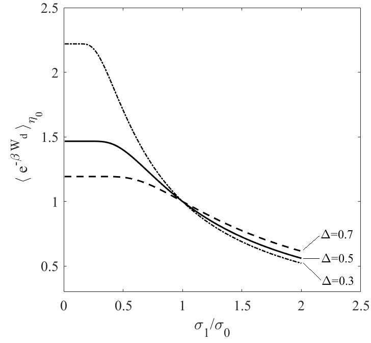
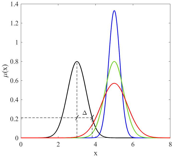
where A=xη0\η1μ1(x)/δ1𝐴subscript𝑥\subscript𝜂0subscript𝜂1subscript𝜇1𝑥subscript𝛿1A=\sum_{x\in\eta_{0}\backslash\eta_{1}}\mu_{1}(x)/\delta_{1} obeys A[0,1]𝐴01A\in[0,1]. It appears that for A𝐴A close to 111, the value eβWdη0subscriptdelimited-⟨⟩superscript𝑒𝛽subscript𝑊𝑑subscript𝜂0\left\langle e^{-\beta W_{d}}\right\rangle_{\eta_{0}} can exceed 1, depending on the values of μ0(x)subscript𝜇0𝑥\mu_{0}(x) and μ1(x)subscript𝜇1𝑥\mu_{1}(x), with xη0𝑥subscript𝜂0x\in\eta_{0}. For simplicity, we illustrate this fact with hypothetical gaussian distributions with standard deviations σ0subscript𝜎0\sigma_{0} and σ1subscript𝜎1\sigma_{1}, centered at x=x¯𝑥¯𝑥x=\bar{x}, for which analytical results are readily obtained, cf. Fig. 2.1. While such gaussians are not directly related to our finite states Markov chains, they may arise as limit cases of finite states processes, which will lead to analogous results. In the case of gaussians, the state space is 𝒮=𝒮\cal S=\mathbb{R}, and the initial truncated space we consider is one interval, η0=[x¯Δ,x¯+Δ]subscript𝜂0¯𝑥Δ¯𝑥Δ\eta_{0}=[\bar{x}-\Delta,\bar{x}+\Delta], of width |η0|=2Δsubscript𝜂02Δ|\eta_{0}|=2\Delta. The top right panel of the figure shows that, for different values of μ¯¯𝜇\bar{\mu} (which is the same for both the initial and the final distributions, as generally assumed throughout this work), values of σ1/σ0<1subscript𝜎1subscript𝜎01\sigma_{1}/\sigma_{0}<1 yield eβWdη0>1subscriptdelimited-⟨⟩superscript𝑒𝛽subscript𝑊𝑑subscript𝜂01\left\langle e^{-\beta W_{d}}\right\rangle_{\eta_{0}}>1.

Another scenario concerns distributions μ0subscript𝜇0\mu_{0} and μ1subscript𝜇1\mu_{1} for which η1η0subscript𝜂1subscript𝜂0\eta_{1}\neq\eta_{0} and ={\mathcal{I}}=\emptyset. In this case, the following bound is found:

eβWd(x)η0=1δ11δ0+11δ0(xη0μ1(x)xη1μ1(x))=11δ0xη0μ1(x)<1subscriptdelimited-⟨⟩superscript𝑒𝛽subscript𝑊𝑑𝑥subscript𝜂01subscript𝛿11subscript𝛿011subscript𝛿0subscript𝑥subscript𝜂0subscript𝜇1𝑥subscript𝑥subscript𝜂1subscript𝜇1𝑥11subscript𝛿0subscript𝑥subscript𝜂0subscript𝜇1𝑥1\displaystyle\left\langle e^{-\beta W_{d}(x)}\right\rangle_{\eta_{0}}=\frac{1-\delta_{1}}{1-\delta_{0}}+\frac{1}{1-\delta_{0}}\left(\sum_{x\in\eta_{0}}\mu_{1}(x)-\sum_{x\in\eta_{1}}\mu_{1}(x)\right)=\frac{1}{1-\delta_{0}}\sum_{x\in\eta_{0}}\mu_{1}(x)<1 (2.12)

The inequality follows from the fact that μ1<μ¯subscript𝜇1¯𝜇\mu_{1}<\bar{\mu} on η0subscript𝜂0\eta_{0}, because =\mathcal{I}=\emptyset, hence

xη0μ1(x)<|η0|μ¯xη0μ0(x)=1δ0subscript𝑥subscript𝜂0subscript𝜇1𝑥subscript𝜂0¯𝜇subscript𝑥subscript𝜂0subscript𝜇0𝑥1subscript𝛿0\sum_{x\in\eta_{0}}\mu_{1}(x)<|\eta_{0}|\bar{\mu}\leq\sum_{x\in\eta_{0}}\mu_{0}(x)=1-\delta_{0}

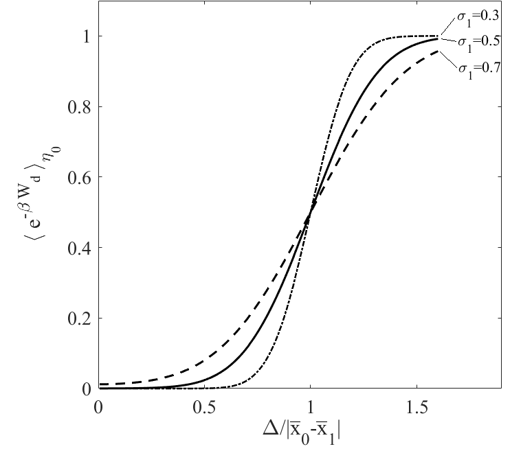
where |η0|subscript𝜂0|\eta_{0}| now represents the cardinality of η0subscript𝜂0\eta_{0}. It is useful to comment on the behavior of the quantity eβWdη0subscriptdelimited-⟨⟩superscript𝑒𝛽subscript𝑊𝑑subscript𝜂0\langle e^{-\beta W_{d}}\rangle_{\eta_{0}} as a function of |η0|subscript𝜂0|\eta_{0}|, whose value can be tuned by varying the cutoff probability μ¯¯𝜇\bar{\mu}. For simplicity, we refer again to gaussian distributions, taking η0=[x¯Δ,x¯+Δ]subscript𝜂0¯𝑥Δ¯𝑥Δ\eta_{0}=[\bar{x}-\Delta,\bar{x}+\Delta], and μ¯¯𝜇\bar{\mu} and ΔΔ\Delta in a range that allows =\mathcal{I}=\emptyset, so that Eq. (2.12) applies. In the bottom left panel of Fig. 2.1 the distributions μ0subscript𝜇0\mu_{0} and μ1subscript𝜇1\mu_{1} are gaussian densities centered at x¯1subscript¯𝑥1\bar{x}_{1} and x¯1x¯0subscript¯𝑥1subscript¯𝑥0\bar{x}_{1}\neq\bar{x}_{0}, with standard deviations σ0subscript𝜎0\sigma_{0} and σ1subscript𝜎1\sigma_{1}, respectively. The bottom right panel of Fig. 2.1 shows that, for values of ΔΔ\Delta guaranteeing =\mathcal{I}=\emptyset, a decrease of ΔΔ\Delta leads to a decrease of eβWdη0subscriptdelimited-⟨⟩superscript𝑒𝛽subscript𝑊𝑑subscript𝜂0\langle e^{-\beta W_{d}}\rangle_{\eta_{0}} to values substantially smaller than 1.

Refer to caption
Refer to caption
Refer to caption
Refer to caption
Figure 2.1: Top row: gaussian distributions centered at x¯0=4subscript¯𝑥04\bar{x}_{0}=4 (left panel): μ0(x)subscript𝜇0𝑥\mu_{0}(x) has standard deviation σ0=0.5subscript𝜎00.5\sigma_{0}=0.5 (black), while the standard deviation of μ1(x)subscript𝜇1𝑥\mu_{1}(x) is σ1=0.3subscript𝜎10.3\sigma_{1}=0.3 (red) and 0.70.70.7 (blue). The horizontal dashed line denotes the value μ¯¯𝜇\bar{\mu}, which determines η0=[x¯0Δ,x¯0+Δ]subscript𝜂0subscript¯𝑥0Δsubscript¯𝑥0Δ\eta_{0}=[\bar{x}_{0}-\Delta,\bar{x}_{0}+\Delta]. Right panel: behavior of eβWdη0subscriptdelimited-⟨⟩superscript𝑒𝛽subscript𝑊𝑑subscript𝜂0\langle e^{-\beta W_{d}}\rangle_{\eta_{0}} as a function of σ1/σ0subscript𝜎1subscript𝜎0\sigma_{1}/\sigma_{0} for different values of ΔΔ\Delta, computed using Eq. (2.12). Bottom row, left panel: μ0(x)subscript𝜇0𝑥\mu_{0}(x) is a gaussian centered at x¯0=3subscript¯𝑥03\bar{x}_{0}=3 with standard deviation σ0=0.5subscript𝜎00.5\sigma_{0}=0.5 (black curve), while μ1(x)subscript𝜇1𝑥\mu_{1}(x) is a gaussian function centered at x¯1=5subscript¯𝑥15\bar{x}_{1}=5 with standard deviations σ1=subscript𝜎1absent\sigma_{1}= 0.3 (blue), 0.5 (green), 0.7 (red). Right panel: graph of eβWdη0subscriptdelimited-⟨⟩superscript𝑒𝛽subscript𝑊𝑑subscript𝜂0\langle e^{-\beta W_{d}}\rangle_{\eta_{0}} as a function of Δ/(x¯0x¯1)Δsubscript¯𝑥0subscript¯𝑥1\Delta/(\bar{x}_{0}-\bar{x}_{1}) for different values of σ1subscript𝜎1\sigma_{1}, computed using Eq. (2.12).

One possible mechanism leading to a reduction of the available state space, is known as absolute irreversibility [18], which is also investigated within the realm of Ising models [22]. Essentially, absolute irreversibility occurs if the probability of a certain “forward” path in the state space is zero, whereas the probability of the corresponding “reverse” path (tracing back in opposite order all the states visited along the forward bath) is non-zero. This phenomenon is experimentally realized when an external field keeps the system first trapped inside a subregion of the state space, and then the constraint is released and the system can explore the whole state space. This is also the case of e.g. the free expansion of a gas, in which particles are initially confined by a wall inside a fraction of the volume of the box and then, after the swift removal of the wall, they can eventually fill up the entire volume. We denote by μ1(x)subscript𝜇1𝑥\mu_{1}(x) and μ0(x)subscript𝜇0𝑥\mu_{0}(x) the probability distributions describing the final and initial states, respectively, that are supported on 𝒮1subscript𝒮1\mathcal{S}_{1} and 𝒮0𝒮1subscript𝒮0subscript𝒮1\mathcal{S}_{0}\subset\mathcal{S}_{1}. In such cases, Eq. (2.5) yields:

eβWd(x)delimited-⟨⟩superscript𝑒𝛽subscript𝑊𝑑𝑥\displaystyle\left\langle e^{-\beta W_{d}(x)}\right\rangle =\displaystyle= x𝒮0μ1(x)<1.subscript𝑥subscript𝒮0subscript𝜇1𝑥1\displaystyle\sum_{x\in\mathcal{S}_{0}}\mu_{1}(x)<1\;. (2.13)

The key aspect of these processes – which encodes much of the physics of the model – is that the state space in the initial state is intrinsically smaller than that in the final state. At times, absolute irreversibility and the state space truncation appear to be interwoven. In Sec. 3.1 we shall discuss a model in which the two phenomena in fact mingle, while =\mathcal{I}=\emptyset. In this case, one finds that

eβWd(x)η0<eβWd(x)<1,subscriptdelimited-⟨⟩superscript𝑒𝛽subscript𝑊𝑑𝑥subscript𝜂0delimited-⟨⟩superscript𝑒𝛽subscript𝑊𝑑𝑥1\left\langle e^{-\beta W_{d}(x)}\right\rangle_{\eta_{0}}<\left\langle e^{-\beta W_{d}(x)}\right\rangle<1\;, (2.14)

where the first inequality holds provided that

x𝒮0\η0μ0(x)xη0μ1(x)<xη0μ0(x)x𝒮0\η0μ1(x)subscript𝑥\subscript𝒮0subscript𝜂0subscript𝜇0𝑥subscript𝑥subscript𝜂0subscript𝜇1𝑥subscript𝑥subscript𝜂0subscript𝜇0𝑥subscript𝑥\subscript𝒮0subscript𝜂0subscript𝜇1𝑥\sum_{x\in\mathcal{S}_{0}\backslash\eta_{0}}\mu_{0}(x)\sum_{x\in\eta_{0}}\mu_{1}(x)<\sum_{x\in\eta_{0}}\mu_{0}(x)\sum_{x\in\mathcal{S}_{0}\backslash\eta_{0}}\mu_{1}(x)

Note, indeed, that the latter inequality can be rewritten as

0<δ0xη0μ1(x)+(1δ0)x𝒮0\η0μ1(x)0subscript𝛿0subscript𝑥subscript𝜂0subscript𝜇1𝑥1subscript𝛿0subscript𝑥\subscript𝒮0subscript𝜂0subscript𝜇1𝑥0<-\delta_{0}\sum_{x\in\eta_{0}}\mu_{1}(x)+(1-\delta_{0})\sum_{x\in\mathcal{S}_{0}\backslash\eta_{0}}\mu_{1}(x)

Next, adding xη0μ1(x)subscript𝑥subscript𝜂0subscript𝜇1𝑥\sum_{x\in\eta_{0}}\mu_{1}(x) on both sides, one obtains

xη0μ1(x)<(1δ0)(xη0μ1(x)+x𝒮0\η0μ1(x))subscript𝑥subscript𝜂0subscript𝜇1𝑥1subscript𝛿0subscript𝑥subscript𝜂0subscript𝜇1𝑥subscript𝑥\subscript𝒮0subscript𝜂0subscript𝜇1𝑥\sum_{x\in\eta_{0}}\mu_{1}(x)<(1-\delta_{0})\left(\sum_{x\in\eta_{0}}\mu_{1}(x)+\sum_{x\in\mathcal{S}_{0}\backslash\eta_{0}}\mu_{1}(x)\right)

hence

11δ0xη0μ1(x)<x𝒮0μ1(x)11subscript𝛿0subscript𝑥subscript𝜂0subscript𝜇1𝑥subscript𝑥subscript𝒮0subscript𝜇1𝑥\frac{1}{1-\delta_{0}}\sum_{x\in\eta_{0}}\mu_{1}(x)<\sum_{x\in\mathcal{S}_{0}}\mu_{1}(x)

which yields the result.

3 The models

In this section we investigate different models for which an explicit analytical solution can be provided. The Jarzynski relation, revisited with the notions of state space reduction and absolute irreversibility introduced in Sec. 2.2, are used to detect possible discontinuous behaviors of an order parameter as a function of an external control parameter. First, a probabilistic urn model, described by a Markov chain, is considered, in which a threshold parameter allows to tune between different steady states. The second model is the classical 2D Ising model subject to an external magnetic field.

3.1 The urn model

The modification of the classical Ehrenfest urn model [23, 20] that we analyze was originally introduced in [19] to understand billiard dynamics comprising a Maxwell demon [24, 25, 26]. It refers to N𝑁N particles initially distributed inside two urns. At each discrete time step one of the two urns is selected with a probability proportional to the number of particles contained in it, and then one of such particles is moved to the other urn, unless a clogging phenomenon stops it. To represent this process, let n(t)𝒮={0,1,,N}𝑛𝑡𝒮01𝑁n(t)\in\mathcal{S}=\{0,1,...,N\} denote the number of particles in one selected urn at time t𝑡t\in\mathbb{N}, and introduce a parameter λ[0,1]𝜆01\lambda\in[0,1], to define a threshold T=λN{0,1,,N}𝑇𝜆𝑁01𝑁T=\lfloor\lambda N\rfloor\in\{0,1,...,N\} which implements the clogging mechanism together with another parameter ϵ[0,1]italic-ϵ01\epsilon\in[0,1]. We then consider the discrete time Markov chain {n(t):t0}conditional-set𝑛𝑡𝑡0\{n(t):t\geq 0\} that obeys the following transition rules:

pn,n+1(t)(T)=NnNϵ1(T),pn,n1(t)(T)=nNϵ2(T)formulae-sequencesubscriptsuperscript𝑝𝑡𝑛𝑛1𝑇𝑁𝑛𝑁subscriptitalic-ϵ1𝑇subscriptsuperscript𝑝𝑡𝑛𝑛1𝑇𝑛𝑁subscriptitalic-ϵ2𝑇p^{(t)}_{n,n+1}(T)=\frac{N-n}{N}\epsilon_{1}(T),\;\;\;p^{(t)}_{n,n-1}(T)=\frac{n}{N}\epsilon_{2}(T) (3.15)

where

ϵ1(T)={ϵ,n<NT1,nNT,ϵ2={1,nTϵ,n>Tformulae-sequencesubscriptitalic-ϵ1𝑇casesitalic-ϵ𝑛𝑁𝑇1𝑛𝑁𝑇subscriptitalic-ϵ2cases1𝑛𝑇italic-ϵ𝑛𝑇\displaystyle\epsilon_{1}(T)=\begin{cases}\epsilon,&n<N-T\\ 1,&n\geq N-T\end{cases},\;\;\;\;\;\epsilon_{2}=\begin{cases}1,&n\leq T\\ \epsilon,&n>T\end{cases} (3.16)

The stationary distributions μλ(n)subscript𝜇𝜆𝑛\mu_{\lambda}(n) of the process take the form [19]:

μλ(n)=1Cλ(Nn){ϵnifnTϵTifT+1nNT1ϵNnifnNTsubscript𝜇𝜆𝑛1subscript𝐶𝜆binomial𝑁𝑛casessuperscriptitalic-ϵ𝑛if𝑛𝑇superscriptitalic-ϵ𝑇if𝑇1𝑛𝑁𝑇1superscriptitalic-ϵ𝑁𝑛if𝑛𝑁𝑇\mu_{\lambda}(n)=\frac{1}{C_{\lambda}}\binom{N}{n}\begin{cases}\epsilon^{n}&\textit{if}\hskip 14.22636ptn\leq T\\ \epsilon^{T}&\textit{if}\hskip 14.22636ptT+1\leq n\leq N-T-1\\ \epsilon^{N-n}&\textit{if}\hskip 14.22636ptn\geq N-T\end{cases} (3.17)

when T<N/2𝑇𝑁2T<N/2, and

μλ(n)=1Cλ(Nn){ϵnifnNT+1ϵNT+1ifNT+2nT1ϵNnifnTsubscript𝜇𝜆𝑛1subscript𝐶𝜆binomial𝑁𝑛casessuperscriptitalic-ϵ𝑛if𝑛𝑁𝑇1superscriptitalic-ϵ𝑁𝑇1if𝑁𝑇2𝑛𝑇1superscriptitalic-ϵ𝑁𝑛if𝑛𝑇\mu_{\lambda}(n)=\frac{1}{C_{\lambda}}\binom{N}{n}\begin{cases}\epsilon^{n}&\textit{if}\hskip 14.22636ptn\geq N-T+1\\ \epsilon^{N-T+1}&\textit{if}\hskip 14.22636ptN-T+2\leq n\leq T-1\\ \epsilon^{N-n}&\textit{if}\hskip 14.22636ptn\leq T\end{cases} (3.18)

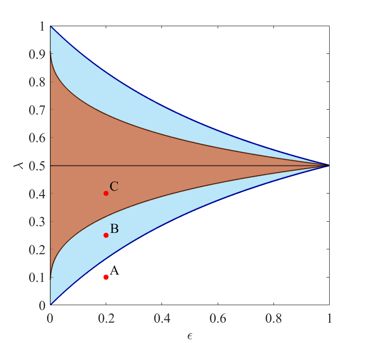
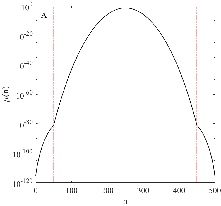
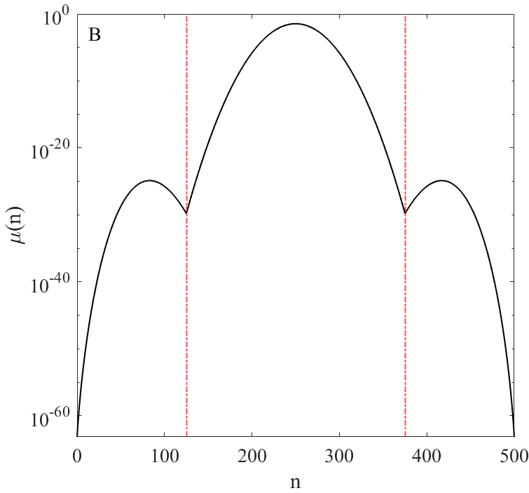
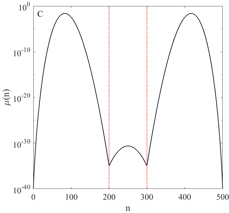
when T>N/2𝑇𝑁2T>N/2, where Cλsubscript𝐶𝜆C_{\lambda} is the normalization coefficient associated to μλsubscript𝜇𝜆\mu_{\lambda}. We only analyze the case T<N/2𝑇𝑁2T<N/2, as the case T>N/2𝑇𝑁2T>N/2 trvially follows. The dependence of the stationary state on the parameters ϵitalic-ϵ\epsilon and λ𝜆\lambda, along with the stationary distribution μ(n)𝜇𝑛\mu(n) evaluated in different regions of the parameter space are shown in Fig. 3.2, showing that μ𝜇\mu concentrates about different states for different values λ𝜆\lambda. In particular, the left panel of Fig. 3.2 reveals the presence, in parameter space, of equilibrium as well as nonequilibrium phases, portrayed as white and brown regions, respectively [19]. While in the equilibrium region the stationary distribution peaks at n=N/2𝑛𝑁2n=N/2 (second panel from left), in the nonequilibrium ones the distribution concentrates around the two states n=n=(εN1)/(ε+1)𝑛superscript𝑛𝜀𝑁1𝜀1n=n^{*}=(\varepsilon N-1)/(\varepsilon+1) and n=Nn𝑛𝑁superscript𝑛n=N-n^{*} (right panel). Moreover, in the light blue region, shown in the left panel, the states n=n𝑛superscript𝑛n=n^{*} and n=Nn𝑛𝑁superscript𝑛n=N-n^{*} are metastable while n=N/2𝑛𝑁2n=N/2 is stable. The distribution corresponding to the latter case shows a global maximum at n=N/2𝑛𝑁2n=N/2 and two symmetric local maxima at n=n𝑛superscript𝑛n=n^{*} and n=Nn𝑛𝑁superscript𝑛n=N-n^{*} (third panel).

Refer to caption
Refer to caption
Refer to caption
Refer to caption
Figure 3.2: Stationary distributions for N=500𝑁500N=500. Right panel: stability regions in the ϵitalic-ϵ\epsilon-λ𝜆\lambda parameter space. White corresponds to stable equilibrium (n=N/2𝑛𝑁2n=N/2); cyan to two metastable nonequilibrium states (n=n,Nn)𝑛superscript𝑛𝑁superscript𝑛(n=n^{*},N-n^{*}) and stable equilibrium; brown to two stable nonequilibrium states and metastable equilibrium. Remaining three panels, from left to right, plot with vertical log\log-scale the stationary distributions (3.17) referring to the points A=(0.2,0.1)𝐴0.20.1A=(0.2,0.1), B=(0.2,0.25)𝐵0.20.25B=(0.2,0.25) and C=(0.2,0.4)𝐶0.20.4C=(0.2,0.4).

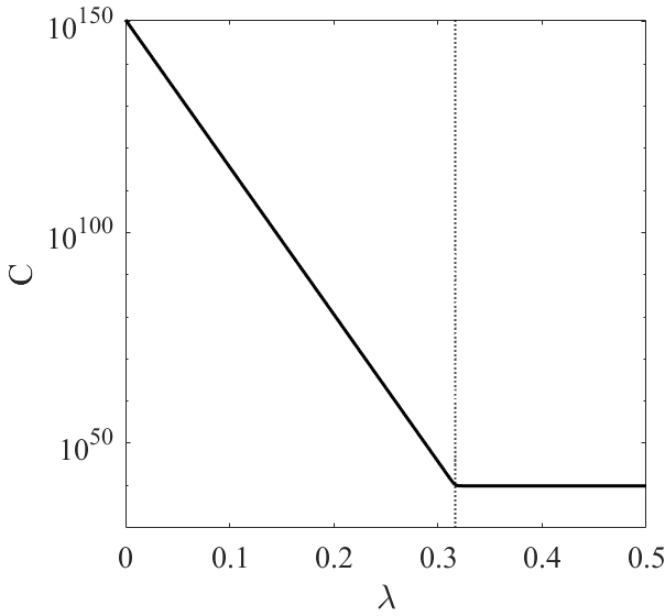
Let us now calculate the normalization coefficient Cλsubscript𝐶𝜆C_{\lambda} and analyze its dependence on the threshold parameter to highlight its singular behavior. First, observe that

Cλsubscript𝐶𝜆\displaystyle C_{\lambda} =\displaystyle= n=0Tϵn(Nn)+n=T+1NT1ϵT(Nn)+n=NTNϵNn(Nn)=2n=0Tϵn(Nn)+n=T+1NT1ϵT(Nn)superscriptsubscript𝑛0𝑇superscriptitalic-ϵ𝑛binomial𝑁𝑛superscriptsubscript𝑛𝑇1𝑁𝑇1superscriptitalic-ϵ𝑇binomial𝑁𝑛superscriptsubscript𝑛𝑁𝑇𝑁superscriptitalic-ϵ𝑁𝑛binomial𝑁𝑛2superscriptsubscript𝑛0𝑇superscriptitalic-ϵ𝑛binomial𝑁𝑛superscriptsubscript𝑛𝑇1𝑁𝑇1superscriptitalic-ϵ𝑇binomial𝑁𝑛\displaystyle\sum_{n=0}^{T}\epsilon^{n}\binom{N}{n}+\sum_{n=T+1}^{N-T-1}\epsilon^{T}\binom{N}{n}+\sum_{n=N-T}^{N}\epsilon^{N-n}\binom{N}{n}=2\sum_{n=0}^{T}\epsilon^{n}\binom{N}{n}+\sum_{n=T+1}^{N-T-1}\epsilon^{T}\binom{N}{n} (3.19)
\displaystyle\approx 2n=0Nϵn(Nn)+n=0NϵT(Nn)=2(1+ϵ)N+2NϵT2superscriptsubscript𝑛0𝑁superscriptitalic-ϵ𝑛binomial𝑁𝑛superscriptsubscript𝑛0𝑁superscriptitalic-ϵ𝑇binomial𝑁𝑛2superscript1italic-ϵ𝑁superscript2𝑁superscriptitalic-ϵ𝑇\displaystyle 2\sum_{n=0}^{N}\epsilon^{n}\binom{N}{n}+\sum_{n=0}^{N}\epsilon^{T}\binom{N}{n}=2(1+\epsilon)^{N}+2^{N}\epsilon^{T}

where the last equality follows from the binomial theorem. Therefore, for ϵ<1italic-ϵ1\epsilon<1 and T>1𝑇1T>1, Cλsubscript𝐶𝜆C_{\lambda} is an exponentially decaying function of λ𝜆\lambda. Moreover, the term (1+ϵ)Nsuperscript1italic-ϵ𝑁(1+\epsilon)^{N} is negligible with respect to 2NϵTsuperscript2𝑁superscriptitalic-ϵ𝑇2^{N}\epsilon^{T} if

T<Nlog(1+ϵ2)(logϵ)1𝑇𝑁1italic-ϵ2superscriptitalic-ϵ1T<N\log\left(\frac{1+\epsilon}{2}\right)(\log\epsilon)^{-1}

while 2NϵTsuperscript2𝑁superscriptitalic-ϵ𝑇2^{N}\epsilon^{T} is negligible with respect to (1+ϵ)Nsuperscript1italic-ϵ𝑁(1+\epsilon)^{N} if

T>Nlog(1+ϵ2)(logϵ)1𝑇𝑁1italic-ϵ2superscriptitalic-ϵ1T>N\log\left(\frac{1+\epsilon}{2}\right)(\log\epsilon)^{-1}

In the large N𝑁N limit, the separation between these two regimes becomes sharp, and defines the critical value [19]

λ=log(1+ϵ2)(logϵ)1superscript𝜆1italic-ϵ2superscriptitalic-ϵ1\lambda^{*}=\log\left(\frac{1+\epsilon}{2}\right)(\log\epsilon)^{-1} (3.20)

of a phase transition, implying:

Cλ<λsubscript𝐶𝜆superscript𝜆\displaystyle C_{\lambda<\lambda^{*}} \displaystyle\approx 2NϵT,superscript2𝑁superscriptitalic-ϵ𝑇\displaystyle 2^{N}\epsilon^{T},
Cλ>λsubscript𝐶𝜆superscript𝜆\displaystyle C_{\lambda>\lambda^{*}} \displaystyle\approx 2(1+ϵ)N.2superscript1italic-ϵ𝑁\displaystyle 2(1+\epsilon)^{N}. (3.21)

The behavior of Cλsubscript𝐶𝜆C_{\lambda} as a function of the normalized threshold λ𝜆\lambda is illustrated in Fig. 3.3.

Mimicking the theory of phase transitions, let us now look at the first derivative with respect to λ𝜆\lambda of the quantity =β1logCsuperscript𝛽1𝐶\mathcal{F}=-\beta^{-1}\log{C}:

M1Nλ=1Nλ(1βlogC(λ))𝑀1𝑁𝜆1𝑁𝜆1𝛽𝐶𝜆M\coloneqq-\frac{1}{N}\frac{\partial}{\partial\lambda}\mathcal{F}=-\frac{1}{N}\frac{\partial}{\partial\lambda}\left(-\frac{1}{\beta}\log{C(\lambda)}\right) (3.22)

which using Eq.(3.19), and taking large N𝑁N so that TλN𝑇𝜆𝑁T\approx\lambda N, writes:

M=logϵβ2NϵλN(1+ϵ)N+2NϵλN=logϵ2β[1+tanh(N2(λλ)logϵ)]𝑀italic-ϵ𝛽superscript2𝑁superscriptitalic-ϵ𝜆𝑁superscript1italic-ϵ𝑁superscript2𝑁superscriptitalic-ϵ𝜆𝑁italic-ϵ2𝛽delimited-[]1𝑁2𝜆superscript𝜆italic-ϵM=\frac{\log{\epsilon}}{\beta}\frac{2^{N}\epsilon^{\lambda N}}{(1+\epsilon)^{N}+2^{N}\epsilon^{\lambda N}}=\frac{\log{\epsilon}}{2\beta}\left[1+\tanh{\left(\frac{N}{2}\left(\lambda-\lambda^{*}\right)\log\epsilon\right)}\right] (3.23)

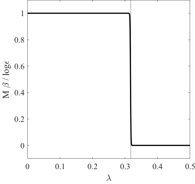
The graph of M(λ)𝑀𝜆M(\lambda), which acts as an order parameter for this model, is shown in the right panel of Fig. 3.3 for N=500𝑁500N=500. At such moderate N𝑁N, hence even more sharply in the large N𝑁N limit, M𝑀M undergoes a jump discontinuity at λ=λ𝜆superscript𝜆\lambda=\lambda^{*}, which in statistical mechanics is typically associated with first order phase transitions.
Refer to caption
Refer to caption
Figure 3.3: Left panel: Normalization constant Cλsubscript𝐶𝜆C_{\lambda} as a function of λ𝜆\lambda, Eq. (3.19), with vertical axis in logarithmic scale. Dotted vertical line indicates the critical value λsuperscript𝜆\lambda^{*} defined in Eq. (3.20). Right panel: M(λ)β/logϵ𝑀𝜆𝛽italic-ϵM(\lambda)\beta/\log{\epsilon} obtained through Eq. (3.23), with dotted vertical line indicating the critical value λsuperscript𝜆\lambda^{*}. Both plots are obtained for N=500𝑁500N=500, β=1𝛽1\beta=1 and ϵ=0.2italic-ϵ0.2\epsilon=0.2.

Suppose now that the threshold depends on time, so that λ=λ(t)𝜆𝜆𝑡\lambda=\lambda(t), with t=0,1𝑡01t=0,1, constitutes a protocol in accord with the theory illustrated in Sect. 2.1, and μλ(t)subscript𝜇𝜆𝑡\mu_{\lambda(t)} is understood as the stationary distribution corresponding to a fixed value of t𝑡t [17]. In particular, take the one-step transformation expressed by the protocol λ0λ1subscript𝜆0subscript𝜆1\lambda_{0}\rightarrow\lambda_{1}, with λ0λ(0)=0subscript𝜆0𝜆00\lambda_{0}\equiv\lambda(0)=0 and λ1λ(1)[0,0.5]subscript𝜆1𝜆100.5\lambda_{1}\equiv\lambda(1)\in[0,0.5]. The associated stationary distributions can be computed using Eq. (3.17) and (3.21). Specifically, denoting by μ0(n)μλ0(n)subscript𝜇0𝑛subscript𝜇subscript𝜆0𝑛\mu_{0}(n)\equiv\mu_{\lambda_{0}}(n) the distribution evaluated at λ=λ0𝜆subscript𝜆0\lambda=\lambda_{0}, we find

μ0(n)=12N(Nn),subscript𝜇0𝑛1superscript2𝑁binomial𝑁𝑛\mu_{0}(n)=\frac{1}{2^{N}}\binom{N}{n}\;,

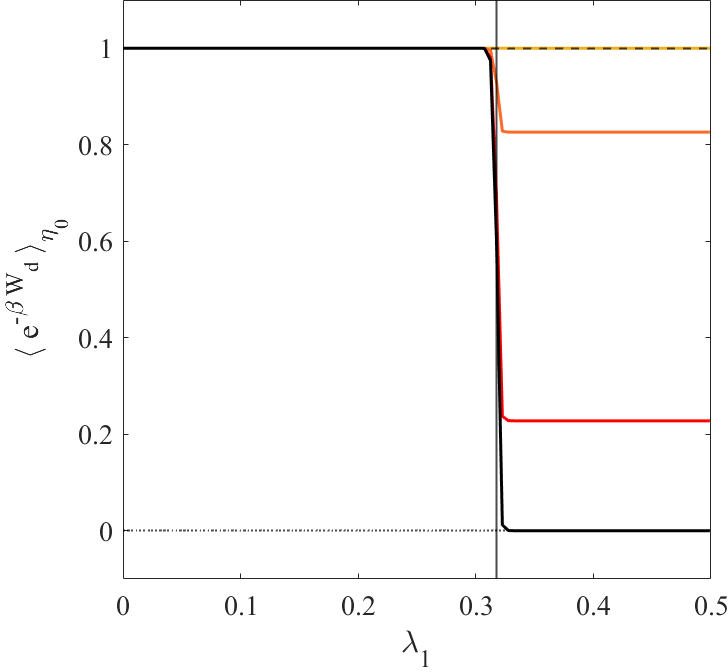
whereas μ1(n)μλ1(n)subscript𝜇1𝑛subscript𝜇subscript𝜆1𝑛\mu_{1}(n)\equiv\mu_{\lambda_{1}}(n) depends on the final value λ1subscript𝜆1\lambda_{1} of the protocol. As discussed earlier in Sec. 2.2, a summation over all possible initial states n𝒮0={0,1,,N}𝑛subscript𝒮001𝑁n\in\mathcal{S}_{0}=\{0,1,...,N\} in Eq. (2.10), which corresponds to no state space reduction (μ¯=0¯𝜇0\bar{\mu}=0), yields the JE, regardless of the chosen value of λ1subscript𝜆1\lambda_{1}. Specifically, for λ<λ10.5superscript𝜆subscript𝜆10.5\lambda^{*}<\lambda_{1}\leq 0.5 two symmetric steady states n=n𝑛superscript𝑛n=n^{*} and n=Nn𝑛𝑁superscript𝑛n=N-n^{*} appear. Indeed, we have 𝒮0=𝒮1={0,1,,N}subscript𝒮0subscript𝒮101𝑁\mathcal{S}_{0}=\mathcal{S}_{1}=\{0,1,\dots,N\}, and Eq. (2.5) applies, independently of λ1subscript𝜆1\lambda_{1}. Therefore, the JE does not reveal the jump discontinuity portrayed in the right panel of Fig. 3.3, because it is not affected by that. The situation is different if the state space is reduced to a subset η0subscript𝜂0\eta_{0} by a cutoff probability μ¯>0¯𝜇0\bar{\mu}>0, see Eq. (2.9). The left panel of Fig. 3.4 shows indeed that eβWdη01similar-to-or-equalssubscriptdelimited-⟨⟩superscript𝑒𝛽subscript𝑊𝑑subscript𝜂01\left\langle e^{-\beta W_{d}}\right\rangle_{\eta_{0}}\simeq 1 for λ1<λsubscript𝜆1superscript𝜆\lambda_{1}<\lambda^{*}, while a sudden drop to a value eβWdη0<1subscriptdelimited-⟨⟩superscript𝑒𝛽subscript𝑊𝑑subscript𝜂01\left\langle e^{-\beta W_{d}}\right\rangle_{\eta_{0}}<1 occurs for λ1>λsubscript𝜆1superscript𝜆\lambda_{1}>\lambda^{*}. In fact, μ¯¯𝜇\bar{\mu} as small as 1020superscript102010^{-20} suffices to get eβWdη00similar-to-or-equalssubscriptdelimited-⟨⟩superscript𝑒𝛽subscript𝑊𝑑subscript𝜂00\left\langle e^{-\beta W_{d}}\right\rangle_{\eta_{0}}\simeq 0 for λ1>λsubscript𝜆1superscript𝜆\lambda_{1}>\lambda^{*}. This behavior signals the sudden separation of the state space regions occupied by the sets η0subscript𝜂0\eta_{0} and η1subscript𝜂1\eta_{1}, in Eq. (2.10), occurring at λ1=λsubscript𝜆1superscript𝜆\lambda_{1}=\lambda^{*}. While for λ1<λsubscript𝜆1superscript𝜆\lambda_{1}<\lambda^{*} the sets η0subscript𝜂0\eta_{0} and η1subscript𝜂1\eta_{1} overlap consistently, for λ1>λsubscript𝜆1superscript𝜆\lambda_{1}>\lambda^{*} one can safely consider =\mathcal{I}=\emptyset, provided μ¯¯𝜇\bar{\mu} is large enough. Thus, following the discussion of Sec. 2.2, for λ1>λsubscript𝜆1superscript𝜆\lambda_{1}>\lambda^{*} one expects not only that eβWdη0<1subscriptdelimited-⟨⟩superscript𝑒𝛽subscript𝑊𝑑subscript𝜂01\left\langle e^{-\beta W_{d}}\right\rangle_{\eta_{0}}<1, but also that, this average decreases for growing μ¯¯𝜇\bar{\mu}. This is indeed demonstrated in the left panel of Fig. 3.4.

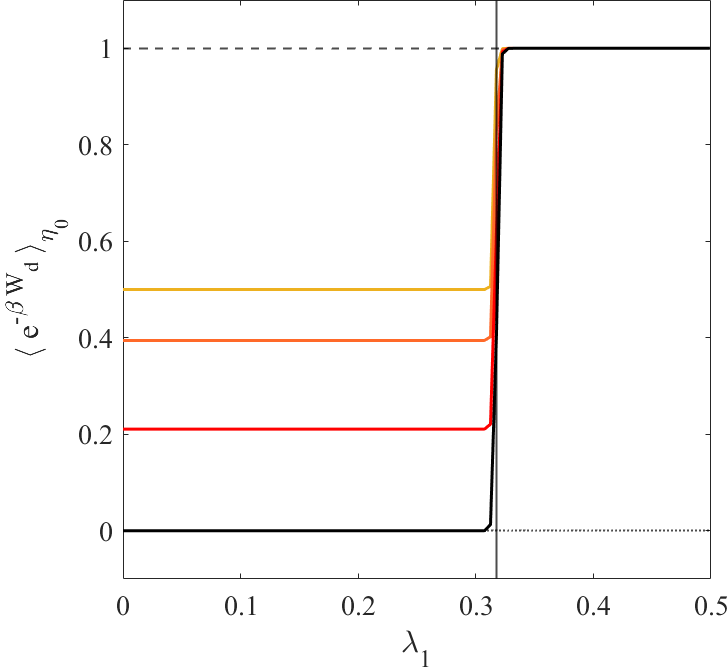
Consider now the one-step transformations with λ0=0.5subscript𝜆00.5\lambda_{0}=0.5, which is larger than λsuperscript𝜆\lambda^{*}, and any λ1[0,1]subscript𝜆101\lambda_{1}\in[0,1]. In this case, the translational symmetry is broken, because the initial condition selects only one of the two nonequilibrium states, say the one with n=n𝑛superscript𝑛n=n^{*}. Then, taking T=N/2𝑇𝑁2T=N/2 in Eq. (3.17) yields

μλ=0.5=1C0.5(Nn)ϵn,n<N/2.formulae-sequencesubscript𝜇𝜆0.51subscript𝐶0.5binomial𝑁𝑛superscriptitalic-ϵ𝑛𝑛𝑁2\mu_{\lambda=0.5}=\frac{1}{C_{0.5}}\binom{N}{n}\epsilon^{n},\;\;n<N/2\;.

where the second row of Eq. (3.21) turns C0.5(1+ϵ)Nsubscript𝐶0.5superscript1italic-ϵ𝑁C_{0.5}\approx(1+\epsilon)^{N}, because only half of the state space 𝒮𝒮\mathcal{S} is involved. One obtains:

μλ(0)(n)={ϵn(1+ϵ)N(Nn)forn<N/20fornN/2subscript𝜇𝜆0𝑛casessuperscriptitalic-ϵ𝑛superscript1italic-ϵ𝑁binomial𝑁𝑛for𝑛𝑁2otherwise0for𝑛𝑁2otherwise\displaystyle\mu_{\lambda(0)}(n)=\begin{cases}\frac{\epsilon^{n}}{(1+\epsilon)^{N}}\binom{N}{n}\;\;\text{for}\;\;n<N/2\\ 0\;\;\text{for}\;\;n\geq N/2\end{cases}

which is supported on 𝒮0={0,,N/21}subscript𝒮00𝑁21\mathcal{S}_{0}=\{0,\dots,N/2-1\}, while the support of the distribution μλ(1)subscript𝜇𝜆1\mu_{\lambda(1)} is 𝒮1=𝒮0subscript𝒮1subscript𝒮0\mathcal{S}_{1}=\mathcal{S}_{0} for λ<λ10.5superscript𝜆subscript𝜆10.5\lambda^{*}<\lambda_{1}\leq 0.5 (nonequilibrium phase) and 𝒮1={0,,N}subscript𝒮10𝑁\mathcal{S}_{1}=\{0,\dots,N\} for 0λ1<λ0subscript𝜆1superscript𝜆0\leq\lambda_{1}<\lambda^{*} (equilibrium phase). Consequently, Eq. (2.5) holds for λ<λ10.5superscript𝜆subscript𝜆10.5\lambda^{*}<\lambda_{1}\leq 0.5 whereas Eq. (2.13) applies for 0λ1<λ0subscript𝜆1superscript𝜆0\leq\lambda_{1}<\lambda^{*}, because 𝒮0𝒮1subscript𝒮0subscript𝒮1\mathcal{S}_{0}\subset\mathcal{S}_{1}, which implies:

eβWd(n)delimited-⟨⟩superscript𝑒𝛽subscript𝑊𝑑𝑛\displaystyle\left\langle e^{-\beta W_{d}(n)}\right\rangle =\displaystyle= n𝒮0μ1(n)=n=0T1ϵn2NϵT(Nn)+n=TN/2112N(Nn)subscript𝑛subscript𝒮0subscript𝜇1𝑛superscriptsubscript𝑛0𝑇1superscriptitalic-ϵ𝑛superscript2𝑁superscriptitalic-ϵ𝑇binomial𝑁𝑛superscriptsubscript𝑛𝑇𝑁211superscript2𝑁binomial𝑁𝑛\displaystyle\sum_{n\in\mathcal{S}_{0}}\mu_{1}(n)=\sum_{n=0}^{T-1}\frac{\epsilon^{n}}{2^{N}\epsilon^{T}}\binom{N}{n}+\sum_{n=T}^{N/2-1}\frac{1}{2^{N}}\binom{N}{n} (3.24)
similar-to-or-equals\displaystyle\simeq n=TN/2112N(Nn)1/2,similar-to-or-equalssuperscriptsubscript𝑛𝑇𝑁211superscript2𝑁binomial𝑁𝑛12\displaystyle\sum_{n=T}^{N/2-1}\frac{1}{2^{N}}\binom{N}{n}\simeq 1/2\;,

where the approximations turn exact for T=0𝑇0T=0 and N𝑁N\rightarrow\infty . The violation of the JE stems from the “absolute irreversibility” of the process λ0λ1subscript𝜆0subscript𝜆1\lambda_{0}\to\lambda_{1}. This is illustrated by the numerical results reported in the right panel of Fig. 3.4, which also clarifies the effect of reducing the state space with a cutoff probability μ¯¯𝜇\bar{\mu}. The effect is a μ¯¯𝜇\bar{\mu} dependent further decrease of the average of eβWdsuperscript𝑒𝛽subscript𝑊𝑑e^{-\beta W_{d}} for 0λ1<λ0subscript𝜆1superscript𝜆0\leq\lambda_{1}<\lambda^{*}, visible in the left panel of Fig. 3.4, cf. Eq. (2.14).

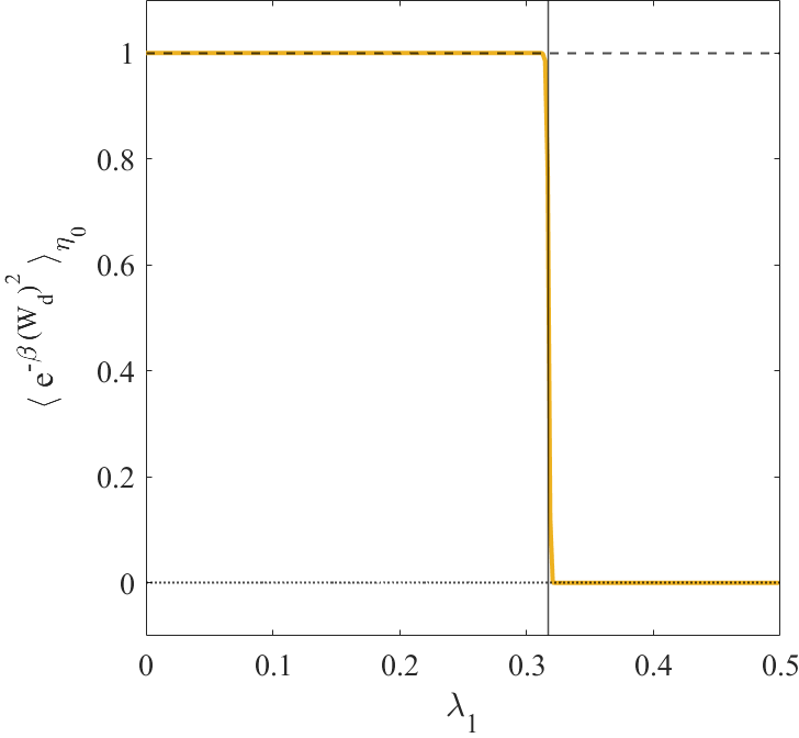
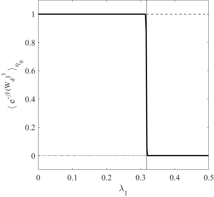
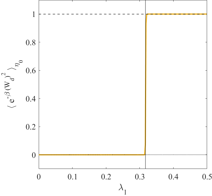
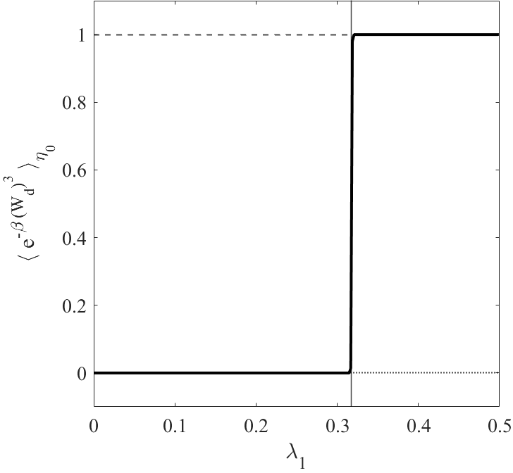
We conclude this Section observing that different exponential variables may be used to efficiently identify phase transitions. For instance, we considered exp{β(Wd)p}𝛽superscriptsubscript𝑊𝑑𝑝\exp\{-\beta\left(W_{d}\right)^{p}\}, with p𝑝p\in\mathbb{N}, and numerically studied the cases p=2𝑝2p=2 and p=3𝑝3p=3. The numerical evaluation of exp{β(Wd)p}η0subscriptdelimited-⟨⟩𝛽superscriptsubscript𝑊𝑑𝑝subscript𝜂0\langle\exp\{-\beta\left(W_{d}\right)^{p}\}\rangle_{\eta_{0}} for the two different values of p𝑝p and for different initial values of λ0subscript𝜆0\lambda_{0} is represented in Fig. 3.5.

It is important to note that, unlike the standard expression, corresponding to p=1𝑝1p=1, the quantity eβ(Wd)2η0subscriptdelimited-⟨⟩superscript𝑒𝛽superscriptsubscript𝑊𝑑2subscript𝜂0\langle e^{-\beta\left(W_{d}\right)^{2}}\rangle_{\eta_{0}} displays a sharp transition at λ=λ𝜆superscript𝜆\lambda=\lambda^{*} even for μ¯=0¯𝜇0\bar{\mu}=0, and not only for the truncated distributions. Moreover, (Wd)2superscriptsubscript𝑊𝑑2\left(W_{d}\right)^{2} is a quantity substantially different from Wdsubscript𝑊𝑑W_{d}, because it only takes non-negative values, while negative values are fundamental for the usual fluctuation relations. This indicates that our approach may result effective with variables of quite different nature.

Let us also note that taking higher odd powers of Wdsubscript𝑊𝑑W_{d}, the calculation of the full state space averages may become prohibitive, from a computational point of view. Indeed, the negative values of Wdsubscript𝑊𝑑W_{d}, raised to a large odd power and exponentiated, may result non-computable. However, our method based on truncated distributions may remain effective, cf. Fig. 3.5 right panel, for p=3𝑝3p=3.

Refer to caption
Refer to caption
Figure 3.4: Numerical estimation of eβWdη0subscriptdelimited-⟨⟩superscript𝑒𝛽subscript𝑊𝑑subscript𝜂0\langle e^{-\beta W_{d}}\rangle_{\eta_{0}}, as a function of λ1subscript𝜆1\lambda_{1}, given by Eq. (2.10). The yellow, orange, red and black lines correspond to cutoffs μ¯=0, 1060, 1050, 1020¯𝜇0superscript1060superscript1050superscript1020\bar{\mu}=0,\;10^{-60},\;10^{-50},\;10^{-20} respectively. The vertical solid black lines lie at λ=λ𝜆superscript𝜆\lambda=\lambda^{*}. The dashed black lines correspond to Eq. (2.5). N𝑁N, β𝛽\beta and ϵitalic-ϵ\epsilon are set to the same values considered in Fig. 3.3. Left panel: The process starts in a homogeneous state with λ0=0subscript𝜆00\lambda_{0}=0. The yellow line is always at 1; the phase transition is only revealed by the truncated distributions. Right panel: the process starts in a non-homogeneous state with λ0=0.5subscript𝜆00.5\lambda_{0}=0.5. The values for μ¯=0¯𝜇0\bar{\mu}=0 and λ<λ𝜆superscript𝜆\lambda<\lambda^{*} do not equal 1, as prescribed by Eq. (3.24). Even the full distribution reveals the phase transition.
Refer to caption
Refer to caption
Refer to caption
Refer to caption
Figure 3.5: Numerical estimation of eβ(Wd)pη0subscriptdelimited-⟨⟩superscript𝑒𝛽superscriptsubscript𝑊𝑑𝑝subscript𝜂0\langle e^{-\beta(W_{d})^{p}}\rangle_{\eta_{0}} as a function of λ1subscript𝜆1\lambda_{1} for p=2𝑝2p=2 and p=3𝑝3p=3 (left and right column, respectively), with the parameters N𝑁N, β𝛽\beta and ϵitalic-ϵ\epsilon set to the same values as in Fig. 3.3. The plots refer to a process starting in a homogeneous state with λ0=0subscript𝜆00\lambda_{0}=0 (top row) or in a non-homogeneous state with λ0=0.5subscript𝜆00.5\lambda_{0}=0.5 (bottom row). In the left panels, the yellow line refers to the cutoff μ¯=0¯𝜇0\bar{\mu}=0, whereas the curves corresponding to cutoff values μ¯>0¯𝜇0\bar{\mu}>0 are not shown in the plots, as they are graphically indistinguishable from the yellow line. In the right panels, the solid black line refers to the cutoff μ¯=1015¯𝜇superscript1015\bar{\mu}=10^{-15}.

3.2 The 2D Ising Model

The second example we tackle is the classical 2D Ising model under an external magnetic field hh, defined on a 222D lattice Λ={1,,L}2Λsuperscript1𝐿2\Lambda=\{1,\dots,L\}^{2}, with the state space 𝒮={1,+1}Λ𝒮superscript11Λ\mathcal{S}=\{-1,+1\}^{\Lambda}. Here β=(kBT)1𝛽superscriptsubscript𝑘𝐵𝑇1\beta=(k_{B}T)^{-1} denotes the inverse temperature. Let σ=(σ1,,σ|Λ|)𝒮𝜎subscript𝜎1subscript𝜎Λ𝒮\mathbf{\sigma}=(\sigma_{1},\dots,\sigma_{|\Lambda|})\in\mathcal{S} denote a generic spin configuration, and introduce the Ising Hamiltonian, which reads

H(σ)=12Jj,kj,kΛσjσkhjΛσj,𝐻𝜎12𝐽subscript𝑗𝑘𝑗𝑘Λsubscript𝜎𝑗subscript𝜎𝑘subscript𝑗Λsubscript𝜎𝑗H(\sigma)=-\frac{1}{2}J\sum_{\begin{subarray}{c}\langle j,k\rangle\\ j,k\in\Lambda\end{subarray}}\sigma_{j}\sigma_{k}-h\sum_{j\in\Lambda}\sigma_{j}\;,

where σj={1,+1}subscript𝜎𝑗11\sigma_{j}=\{-1,+1\} for jΛ𝑗Λj\in\Lambda, J>0𝐽0J>0 denotes the ferromagnetic coupling constant and the first sum is taken over all nearest neighbor spins. Periodic boundary conditions are imposed along the horizontal and vertical directions. The model exhibits a critical value βc=ln(1+2)/2Jsubscript𝛽𝑐122𝐽\beta_{c}=\ln{(1+\sqrt{2})}/2J, marking the transition from a disordered (paramagnetic) to an ordered (ferromagnetic) phase. We then let the the magnetic field depend on time, defining a protocol λ(t)=h(t)𝜆𝑡𝑡\lambda(t)=h(t). In Ref. [22], a similar problem is investigated, taking λ(t)=J(t)𝜆𝑡𝐽𝑡\lambda(t)=J(t). We denote by Hi(σ)subscript𝐻𝑖𝜎H_{i}(\sigma) and Hf(σ)subscript𝐻𝑓𝜎H_{f}(\sigma) the Hamiltonians evaluated at the initial and the final values of the protocol, respectively, and we take μk(σ)=exp(βHk(σ))/Zisubscript𝜇𝑘𝜎𝛽subscript𝐻𝑘𝜎subscript𝑍𝑖\mu_{k}(\sigma)=\exp{(-\beta H_{k}(\sigma))}/Z_{i} as the Gibbs measure at the inverse temperature β𝛽\beta, with k=0,1𝑘01k=0,1 and Zk=σ𝒮exp(βHk(σ))subscript𝑍𝑘subscript𝜎𝒮𝛽subscript𝐻𝑘𝜎Z_{k}=\sum_{\sigma\in\mathcal{S}}\exp{(-\beta H_{k}(\sigma))}. So both μ0subscript𝜇0\mu_{0} and μ1subscript𝜇1\mu_{1} are supported on 𝒮𝒮\mathcal{S}.

We now introduce the reduced state spaces η0={σ|μ0(σ)μ¯}subscript𝜂0conditional-set𝜎subscript𝜇0𝜎¯𝜇\eta_{0}=\{\sigma|\mu_{0}(\sigma)\geq\bar{\mu}\} and η1={σ|μ1(σ)μ¯}subscript𝜂1conditional-set𝜎subscript𝜇1𝜎¯𝜇\eta_{1}=\{\sigma|\mu_{1}(\sigma)\geq\bar{\mu}\} and we correspondingly denote Z¯0=ση0exp(βH0(σ))subscript¯𝑍0subscript𝜎subscript𝜂0𝛽subscript𝐻0𝜎\overline{Z}_{0}=\sum_{\sigma\in\eta_{0}}\exp{(-\beta H_{0}(\sigma))} and Z¯1=ση1exp(βH1(σ))subscript¯𝑍1subscript𝜎subscript𝜂1𝛽subscript𝐻1𝜎\overline{Z}_{1}=\sum_{\sigma\in\eta_{1}}\exp{(-\beta H_{1}(\sigma))}. With the notation of Sec. 2.2, we have:

1δk=σηkμk(σ)=σηkexp(βHk(σ))σ𝒮exp(βHk(σ))=Z¯kZk,k=0,1,formulae-sequence1subscript𝛿𝑘subscript𝜎subscript𝜂𝑘subscript𝜇𝑘𝜎subscript𝜎subscript𝜂𝑘𝛽subscript𝐻𝑘𝜎subscript𝜎𝒮𝛽subscript𝐻𝑘𝜎subscript¯𝑍𝑘subscript𝑍𝑘𝑘011-\delta_{k}=\sum_{\sigma\in\eta_{k}}\mu_{k}(\sigma)=\frac{\sum_{\sigma\in\eta_{k}}\exp{(-\beta H_{k}(\sigma))}}{\sum_{\sigma\in\mathcal{S}}\exp{(-\beta H_{k}(\sigma))}}=\frac{\overline{Z}_{k}}{Z_{k}}\;,\quad k=0,1\;, (3.25)

which yields:

Z¯0Z¯1=Z0Z11δ01δ1.subscript¯𝑍0subscript¯𝑍1subscript𝑍0subscript𝑍11subscript𝛿01subscript𝛿1\displaystyle\frac{\overline{Z}_{0}}{\overline{Z}_{1}}=\frac{Z_{0}}{Z_{1}}\frac{1-\delta_{0}}{1-\delta_{1}}\;.

Furthermore, for a function f(σ):𝒮:𝑓𝜎𝒮f(\sigma):\mathcal{S}\rightarrow\mathbb{R}, we set:

fη0=ση0f(σ)eβH0(σ)Z¯0=11δ0ση0f(σ)μ0(σ).subscriptdelimited-⟨⟩𝑓subscript𝜂0subscript𝜎subscript𝜂0𝑓𝜎superscript𝑒𝛽subscript𝐻0𝜎subscript¯𝑍011subscript𝛿0subscript𝜎subscript𝜂0𝑓𝜎subscript𝜇0𝜎\langle f\rangle_{\eta_{0}}=\sum_{\sigma\in\eta_{0}}f(\sigma)\frac{e^{-\beta H_{0}(\sigma)}}{\overline{Z}_{0}}=\frac{1}{1-\delta_{0}}\sum_{\sigma\in\eta_{0}}f(\sigma)\mu_{0}(\sigma)\;. (3.26)

Then, taking

f(σ)=eβWd=eβ(WΔF)=eβ(H1(σ)H0(σ))Z0Z1,whereβΔF=logZ0Z1,formulae-sequence𝑓𝜎superscript𝑒𝛽subscript𝑊𝑑superscript𝑒𝛽𝑊Δ𝐹superscript𝑒𝛽subscript𝐻1𝜎subscript𝐻0𝜎subscript𝑍0subscript𝑍1where𝛽Δ𝐹continued-fractionsubscript𝑍0subscript𝑍1f(\sigma)=e^{-\beta W_{d}}=e^{-\beta(W-\Delta F)}=e^{-\beta(H_{1}(\sigma)-H_{0}(\sigma))}\frac{Z_{0}}{Z_{1}}\;,\quad\mbox{where}~{}~{}\beta\Delta F=\log\cfrac{Z_{0}}{Z_{1}}\;,

we find

f(σ)μ0(σ)=eβH1(σ)Z0Z0Z1=μ1(σ),𝑓𝜎subscript𝜇0𝜎superscript𝑒𝛽subscript𝐻1𝜎subscript𝑍0subscript𝑍0subscript𝑍1subscript𝜇1𝜎f(\sigma)\mu_{0}(\sigma)=\frac{e^{-\beta H_{1}(\sigma)}}{Z_{0}}\frac{Z_{0}}{Z_{1}}=\mu_{1}(\sigma)\;,

and

eβWdη0=11δ0ση0μ1(σ).subscriptdelimited-⟨⟩superscript𝑒𝛽subscript𝑊𝑑subscript𝜂011subscript𝛿0subscript𝜎subscript𝜂0subscript𝜇1𝜎\displaystyle\left\langle e^{-\beta W_{d}}\right\rangle_{\eta_{0}}=\frac{1}{1-\delta_{0}}\sum_{\sigma\in\eta_{0}}\mu_{1}(\sigma)\;. (3.27)

The latter equation coincides with Eq. (2.10) and recovers [22, Eq. 141414].

We are interested in studying the application of Eq. (3.27) to evolutions in which the magnetic field changes from λ0=h0subscript𝜆0subscript0\lambda_{0}=h_{0} to λ1=h1subscript𝜆1subscript1\lambda_{1}=h_{1}.

Setting J=1𝐽1J=1, which yields βc0.4406subscript𝛽𝑐0.4406\beta_{c}\approx 0.4406, we consider different scenarios. We first choose β>βc𝛽subscript𝛽𝑐\beta>\beta_{c}, so that the 2D Ising model undergoes a first order phase transition when the magnetic field hh changes sign, and we study the behavior of eβWdη0subscriptdelimited-⟨⟩superscript𝑒𝛽subscript𝑊𝑑subscript𝜂0\langle e^{-\beta W_{d}}\rangle_{\eta_{0}} as a function of h1subscript1h_{1}. Later, we study the case with β<βc𝛽subscript𝛽𝑐\beta<\beta_{c}, where no phase transition takes place. The computation of eβWdη0subscriptdelimited-⟨⟩superscript𝑒𝛽subscript𝑊𝑑subscript𝜂0\langle e^{-\beta W_{d}}\rangle_{\eta_{0}} can be conveniently carried out by sampling configurations σ𝒮𝜎𝒮\sigma\in\mathcal{S}, with a prescribed magnetization density m=N1jΛσj𝑚superscript𝑁1subscript𝑗Λsubscript𝜎𝑗m=N^{-1}\sum_{j\in\Lambda}\sigma_{j}, from the distribution [22]:

P(m)=σ𝒮μ(σ)δ(m1NjΛσjΛ)𝑃𝑚subscript𝜎𝒮𝜇𝜎𝛿𝑚1𝑁subscript𝑗Λsubscript𝜎𝑗ΛP(m)=\sum_{\sigma\in\mathcal{S}}\mu(\sigma)\,\delta\left(m-\frac{1}{N}\sum_{j\in\Lambda}\sigma_{j\in\Lambda}\right)
Refer to caption
Refer to caption
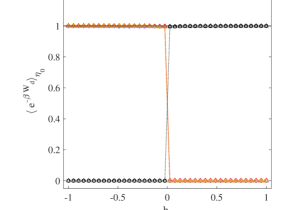
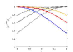
Figure 3.6: eβWdη0subscriptdelimited-⟨⟩superscript𝑒𝛽subscript𝑊𝑑subscript𝜂0\langle e^{-\beta W_{d}}\rangle_{\eta_{0}} as a function of hfsubscript𝑓h_{f}, Eq.  (2.11), from Monte Carlo simulations of a 2D Ising model on a square grid of linear size L=10𝐿10L=10. Here, J=1𝐽1J=1, hence βc0.4406similar-to-or-equalssubscript𝛽𝑐0.4406\beta_{c}\simeq 0.4406, and periodic boundary conditions are applied on both horizontal and vertical directions. Simulations have been performed with hi=1subscript𝑖1h_{i}=-1 (coloured symbols) and hi=1subscript𝑖1h_{i}=1 (black symbols), for β=2.5>βc𝛽2.5subscript𝛽𝑐\beta=2.5>\beta_{c} (left panel) and β=0.1<βc𝛽0.1subscript𝛽𝑐\beta=0.1<\beta_{c} (right panel). Circles, triangles and squares correspond to μ¯=(max{μ0}+max{μ1})/(2k)¯𝜇subscript𝜇0subscript𝜇12𝑘\bar{\mu}=(\max\{\mu_{0}\}+\max\{\mu_{1}\})/(2k) with k=5,25,100𝑘525100k=5,25,100, respectively. The horizontal black line at 111 represents in both panels the case with μ¯=0¯𝜇0\bar{\mu}=0.

Figure 3.6 shows that eβWd=1delimited-⟨⟩superscript𝑒𝛽subscript𝑊𝑑1\langle e^{-\beta W_{d}}\rangle=1 when μ¯=0¯𝜇0\bar{\mu}=0, for both β<βc𝛽subscript𝛽𝑐\beta<\beta_{c} and β>βc𝛽subscript𝛽𝑐\beta>\beta_{c}, cf. Eq. (2.5). Therefore, the phase transition in the Ising model is not detected by the JE in one-step transformations. For the reduced the state spaces, corresponding to cutoffs μ¯>0¯𝜇0\bar{\mu}>0, the situation changes as evidenced by the left panel of Fig. 3.6. The phase transition is properly captured by eβWdη0subscriptdelimited-⟨⟩superscript𝑒𝛽subscript𝑊𝑑subscript𝜂0\langle e^{-\beta W_{d}}\rangle_{\eta_{0}}, which drops abruptly from the value 111 to a value close to 00 when crossing h1=0subscript10h_{1}=0, for h0=1subscript01h_{0}=-1 and with h1[1,1]subscript111h_{1}\in[-1,1]. An analogous behavior is also observed when h0=1subscript01h_{0}=1 and h1subscript1h_{1} is varied in the same interval. It is worth recalling that, in the Curie-Weiss approximation of the Ising model, the value of the magnetization density m𝑚m is obtained from the solution of the mean field equation m=tanh[β(m+h)]𝑚𝛽𝑚m=\tanh{[\beta(m+h)]}, which, for β>βc𝛽subscript𝛽𝑐\beta>\beta_{c}, gives rise to metastable branches [27]. One such branch corresponds to positive values of m𝑚m in the interval [hc,0]subscript𝑐0[-h_{c},0], and another branch corresponds, symmetrically, to negative values of m𝑚m in the interval [0,hc]0subscript𝑐[0,h_{c}], with hc>0subscript𝑐0h_{c}>0. This is not visible in the left panel of Fig. 3.6, which shows that for h0=±1subscript0plus-or-minus1h_{0}=\pm 1 the discontinuity occurs in both cases sharply at h1=0subscript10h_{1}=0. This is a consequence of our choice of initial datum for the Monte Carlo simulations, that mitigates the effects of the two metastable branches. More precisely, as initial datum we took σj=1subscript𝜎𝑗1\sigma_{j}=-1 for h1<0subscript10h_{1}<0 and σj=1subscript𝜎𝑗1\sigma_{j}=1 for h1>0subscript10h_{1}>0, for all jΛ𝑗Λj\in\Lambda, producing a distribution P(m)𝑃𝑚P(m) sharply concentrated near m=1𝑚1m=-1 for h1<0subscript10h_{1}<0 and near m=1𝑚1m=1 for h1>0subscript10h_{1}>0. The discontinuity at h1=0subscript10h_{1}=0 therefore stems from Eq. (2.12), which rules the behavior of eβWdη0subscriptdelimited-⟨⟩superscript𝑒𝛽subscript𝑊𝑑subscript𝜂0\langle e^{-\beta W_{d}}\rangle_{\eta_{0}} for β>βc𝛽subscript𝛽𝑐\beta>\beta_{c}, where one can assume =\mathcal{I}=\emptyset.

In the left panel it is also interesting to note that, for β=2.5>βc𝛽2.5subscript𝛽𝑐\beta=2.5>\beta_{c}, the different sets of data points corresponding to different values of μ¯¯𝜇\bar{\mu} fully overlap with one another and display the same discontinuity at h1=0subscript10h_{1}=0.

For β<βc𝛽subscript𝛽𝑐\beta<\beta_{c} the phase transition in the Ising model is instead absent, and the magnetization density m𝑚m solving the mean field equation becomes a continuous function of hh, that vanishes at h=00h=0. As a result, the data points shown in the right panel of Fig. 3.6 show that eβWdη0subscriptdelimited-⟨⟩superscript𝑒𝛽subscript𝑊𝑑subscript𝜂0\langle e^{-\beta W_{d}}\rangle_{\eta_{0}} no longer presents a sharp discontinuity at h1=0subscript10h_{1}=0, as this quantity decreases in a continuous fashion while increasing the difference |h0h1|subscript0subscript1|h_{0}-h_{1}|. The effect of varying the value of μ¯¯𝜇\bar{\mu} is clearly visible in the right panel. Again, the JE is not affected by the variation of h1subscript1h_{1}.

4 Conclusions

In this study, we propose one way of benefiting from incomplete statistics or finite size effects, that result in a reduction of the state space. As this is often an unavoidable fact, we show that it can provide valuable insight, if associated with exponential observables. In particular, we have considered the Jarzynski Equality and its instantaneous transformation variant (also known as Free Energy Perturbation), to identify the critical values of the parameters corresponding to a first order phase transition. Smooth variations of states have also been characterized. This is due to the sensitivity of exponentials of extensive quantities, when averaged over the available subsets of the system state space, which is usually considered a hindrance.

Interestingly enough, our study show that reducing the amount of available information about the system can enhance our understanding of its critical behaviors. In fact, this is not obtained from a perfect sampling of states. The JE, in particular, results insensitive to parameters variations, hiding interesting features of the system at hand.

We illustrated our theoretical findings numerically analyzing two stochastic models: a modified Ehrenfest urn model and a classical 2D Ising model subject to an external magnetic field. In both cases, we observed a jump discontinuity in the quantity eβWdη0subscriptdelimited-⟨⟩superscript𝑒𝛽subscript𝑊𝑑subscript𝜂0\langle e^{-\beta W_{d}}\rangle_{\eta_{0}} occurring at the same value of the control parameter distinguishing different macroscopic phases in the thermodynamic limit of the model, remaining quite far from that limit. Similarly, when the phase transition is absent, as in the case of the Ising model at supercritical temperatures, the variation of state with the control parameter, is still revealed by a continuous variation of eβWdη0subscriptdelimited-⟨⟩superscript𝑒𝛽subscript𝑊𝑑subscript𝜂0\langle e^{-\beta W_{d}}\rangle_{\eta_{0}}.

Studying the behaviour of powers of Wdsubscript𝑊𝑑W_{d} we also found that our approach works even with variables different from those of fluctuation theorems. Indeed, it provides a new recipe to identify order parameters in the study of nonequilibrium phase transitions, that is particularly effective with truncated distributions.

Future works are intended to develop this approach, so that incomplete information on a given system may be used beyond the problem of discovering phase transitions.

Acknowledgements LR gratefully acknowledges support from the Italian Ministry of University and Research (MUR) through the grant PRIN2022-PNRR project (No. P2022Z7ZAJ) “A Unitary Mathematical Framework for Modelling Muscular Dystrophies” (CUP: E53D23018070001). This work has been performed under the auspices of Italian National Group of Mathematical Physics (GNFM) of the Istituto Nazionale di Alta Matematica (INdAM).

References

  • [1] C. H. Bennett, “Efficient estimation of free energy differences from monte carlo data,” Journal of Computational Physics, vol. 22, no. 2, pp. 245–268, 1976.
  • [2] B. Widom, “Some topics in the theory of fluids,” The Journal of Chemical Physics, vol. 39, no. 11, pp. 2808–2812, 1963.
  • [3] R. W. Zwanzig, “High-temperature equation of state by a perturbation method. ii. polar gases,” The Journal of Chemical Physics, vol. 23, no. 10, pp. 1915–1922, 1955.
  • [4] D. J. Evans, E. G. D. Cohen, and G. P. Morriss, “Probability of second law violations in shearing steady states,” Physical review letters, vol. 71, no. 15, p. 2401, 1993.
  • [5] O. G. Jepps and L. Rondoni, “A dynamical-systems interpretation of the dissipation function, t-mixing and their relation to thermodynamic relaxation,” Journal of Physics A: Mathematical and Theoretical, vol. 49, no. 15, p. 154002, 2016.
  • [6] C. Jarzynski, “Nonequilibrium equality for free energy differences,” Physical Review Letters, vol. 78, no. 14, p. 2690, 1997.
  • [7] G. E. Crooks, “Nonequilibrium measurements of free energy differences for microscopically reversible markovian systems,” Journal of Statistical Physics, vol. 90, pp. 1481–1487, 1998.
  • [8] G. E. Crooks, “Path-ensemble averages in systems driven far from equilibrium,” Phys. Rev. E, vol. 61, pp. 2361–2366, Mar 2000.
  • [9] T. Hatano and S.-i. Sasa, “Steady-state thermodynamics of langevin systems,” Physical review letters, vol. 86, no. 16, p. 3463, 2001.
  • [10] U. M. B. Marconi, A. Puglisi, L. Rondoni, and A. Vulpiani, “Fluctuation–dissipation: response theory in statistical physics,” Physics reports, vol. 461, no. 4-6, pp. 111–195, 2008.
  • [11] U. Seifert, “Stochastic thermodynamics, fluctuation theorems and molecular machines,” Reports on Progress in Physics, vol. 75, p. 126001, nov 2012.
  • [12] N. Hansen and W. F. Van Gunsteren, “Practical aspects of free-energy calculations: a review,” Journal of chemical theory and computation, vol. 10, no. 7, pp. 2632–2647, 2014.
  • [13] G. M. Torrie and J. P. Valleau, “Nonphysical sampling distributions in monte carlo free-energy estimation: Umbrella sampling,” Journal of Computational Physics, vol. 23, no. 2, pp. 187–199, 1977.
  • [14] A. Pohorille, C. Jarzynski, and C. Chipot, “Good practices in free-energy calculations,” The Journal of Physical Chemistry B, vol. 114, no. 32, pp. 10235–10253, 2010.
  • [15] D. Wu and D. A. Kofke, “Phase-space overlap measures. ii. design and implementation of staging methods for free-energy calculations,” The Journal of chemical physics, vol. 123, no. 8, 2005.
  • [16] M. Colangeli, A. Di Francesco, and L. Rondoni, “Finite reservoirs corrections to hamiltonian systems statistics and time symmetry breaking,” Symmetry, vol. 15, no. 6, p. 1268, 2023.
  • [17] P. Hack, S. Gottwald, and D. A. Braun, “Jarzyski’s equality and crooks’ fluctuation theorem for general markov chains with application to decision-making systems,” Entropy, vol. 42, p. 1731, 2022.
  • [18] Y. Murashita, K. Funo, and M. Ueda, “Nonequilibrium equalities in absolutely irreversible processes,” Physical Review E, vol. 90, no. 4, p. 042110, 2014.
  • [19] E. N. Cirillo, M. Colangeli, A. Muntean, O. Richardson, and L. Rondoni, “Deterministic reversible model of non-equilibrium phase transitions and stochastic counterpart,” Journal of Physics A: Mathematical and Theoretical, vol. 53, no. 30, p. 305001, 2020.
  • [20] W. Feller, An Introduction to Probability. Theory and Applications. John Wiley & Sons, 1968.
  • [21] K. Sekimoto, Stochastic Energetics. Springer Berlin, Heidelberg, 2010.
  • [22] D.-T. Hoang, B. Prasanna Venkatesh, S. Han, J. Jo, G. Watanabe, and M.-S. Choi, “Scaling law for irreversible entropy production in critical systems,” Scientific reports, vol. 6, no. 1, p. 27603, 2016.
  • [23] M. Kac, Probability and Related Topics in Physical Sciences, vol. 1 of Lectures in Applied Mathematics. Interscience Publishers, 1959.
  • [24] E. N. Cirillo, M. Colangeli, O. Richardson, and L. Rondoni, “Deterministic model of battery, uphill currents, and nonequilibrium phase transitions,” Physical Review E, vol. 103, no. 3, p. 032119, 2021.
  • [25] E. N. Cirillo, M. Colangeli, A. Di Francesco, M. Kröger, and L. Rondoni, “Transport and nonequilibrium phase transitions in polygonal urn models,” Chaos: An Interdisciplinary Journal of Nonlinear Science, vol. 32, no. 9, p. 093127, 2022.
  • [26] E. N. Cirillo, M. Colangeli, M. Kröger, and L. Rondoni, “Nonequilibrium phase transitions in feedback-controlled three-dimensional particle dynamics,” Physical Review Research, vol. 5, p. 043063, 2023.
  • [27] E. Presutti, Scaling Limits in Statistical Mechanics and Microstructures in Continuum Mechanics. Springer Berlin, Heidelberg, 2009.