Powerformer: A Section-adaptive Transformer for Power Flow Adjustment
Abstract
In this paper, we present a novel transformer architecture tailored for learning robust power system state representations, which strives to optimize power dispatch for the power flow adjustment across different transmission sections. Specifically, our proposed approach, named Powerformer, develops a dedicated section-adaptive attention mechanism, separating itself from the self-attention used in conventional transformers. This mechanism effectively integrates power system states with transmission section information, which facilitates the development of robust state representations. Furthermore, by considering the graph topology of power system and the electrical attributes of bus nodes, we introduce two customized strategies to further enhance the expressiveness: graph neural network propagation and multi-factor attention mechanism. Extensive evaluations are conducted on three power system scenarios, including the IEEE 118-bus system, a realistic 300-bus system in China, and a large-scale European system with 9241 buses, where Powerformer demonstrates its superior performance over several baseline methods.
keywords:
graph neural network, power flow adjustment, power system state representation learning, section-adaptive attention, transformerChen et al.: Powerformer: A Section-adaptive Transformer for Power Flow Adjustment
Graph Abstract:
![[Uncaptioned image]](/html/2401.02771/assets/x1.png)
[label1]organization=College of Computer Science and Technology, Zhejiang University,postcode=310027, state=Hangzhou, country=China \affiliation[label2]organization=Polytechnic Institute, Zhejiang University,postcode=310027, state=Hangzhou, country=China \affiliation[label3]organization=College of Software, Zhejiang University,postcode=315000, state=Ningbo, country=China \affiliation[label4]organization=College of Electrical Engineering, Zhejiang University,postcode=310027, state=Hangzhou, country=China
1 Introduction
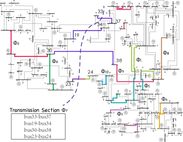
Power flow adjustment across the transmission sections refers to manage and regulate the power flow between two system components or entities. As shown in Fig. 1, a transmission section consists of a group of transmission lines with the same color that have the same direction of active power flow and are closely located electrically. In a real-world scenario, the power demand in China’s northern area drastically increases due to the arrival of winter, and the power generation in this area falls insufficient, making it necessary to transfer power from the southern to the northern through the transmission section. To ensure power system security margins, operators commonly employ the total transfer capability of the transmission section to monitor power flows and regulate the operational state [1, 2, 3]. Specifically, overloading a critical transmission section poses a serious threat to the system, potentially triggering a chain reaction of failures that may cause severe cascading blackouts. Hence, the efficient management of power flow at transmission sections is paramount, serving as a fundamental pillar to ensure the stability, resilience, and reliability of the power system.
To address power flow adjustment across different transmission sections, power dispatch is an effective strategy that enables precise finetuning of generation outputs to optimize power flow distribution. Traditional dispatch methods, which rely on the system model, can be primarily categorized into two distinct classes: optimization-based [4] and sensitivity-based [5] techniques. Optimization-based methods utilize numerical techniques to transform the dispatch problem into a constrained programming problem, while sensitivity-based methods apply iterative calculations to find candidate generators by calculating sensitivity indices. However, these model-based methods often encounter the computational burdens and struggle to effectively control unpredictable system coupling within a limited time. Thus, traditional methods are unsuitable for effectively managing real-time control in a complex and large-scale power system.
Recently, deep reinforcement learning (DRL) has emerged as an innovative alternative to traditional power dispatch methods. This data-driven approach effectively utilizes the robust capabilities of the pertained deep neural networks, enabling the direct learning of response actions in an end-to-end fashion, effectively tackling the high-dimensional control problems and providing a powerful solution for power flow adjustment. However, among the existing DRL methods [6, 7], there are two evident limitations in the state representations for section power flow adjustment:
-
1.
The absence of efficient awareness regarding transmission sections, which hinders the DRL agent from making optimal action for distinct section adjustment.
-
2.
The high coupled electrical factors and the ignored topology structure of power system, ignificantly affect the extraction of the state characteristics.
In this paper, we strive to develop an advanced transformer architecture for learning robust power system state representations, enabling the DRL agent to perform precise power dispatch strategies that stabilize the power system under various section settings. To tackle the first limitation, we develop a section-adaptive attention mechanism to enable an efficient amalgamation of section information with the power system state, leveraging the comprehensive capabilities of the transformer architecture [8, 9, 10] for the specific sectional system analysis. For the second limitation, we begin by analyzing the graph topology of the power system, and employing graph neural networks [11, 12, 13] to propagate features for embedding structural information into state representations. Furthermore, we introduce a multi-factor attention mechanism to efficiently fuse each state factor, ensuring comprehensive and accurate extraction of system states. Finally, we utilize the proposed Powerformer, integrating the Dueling DQN [14] framework to achieve precise and efficient control of power flow across transmission sections, thereby leading to improvements in the overall system performance.
To the best of our knowledge, this is the first Transformer architecture that attempts to amalgamate the section information with state representation for transmission section power flow adjustment. Our main contributions can be summarized as follows:
-
1.
We develop a section-adaptive attention mechanism that effectively integrates power system state features and section power flow information to achieve the knowledge amalgamation for different transmission sections.
-
2.
We introduce graph neural networks propagation alongside a multi-factor attention mechanism, specifically tailored to fuse the power system’s graph topology information and effectively emerge electrical state factors.
-
3.
Extensive evaluation on three distinct power system cases, including the IEEE 118-bus system, a realistic 300-bus system in China, and a large-scale 9241-bus European system, demonstrates our method’s superiority over several baselines with significantly improved performance.
2 PRELIMINARY
2.1 Problem Formulation and Task Setting
2.1.1 Problem Formulation
Transmission section power flow adjustment involves the regulation and control of electrical power flow through the specific section or interface of a power transmission network. In a specific power system, there exist transmission sections , where each section consists of several transmission lines that not only share the same direction of active power flow but also maintain close electrical proximity to one another [15]. To accurately determine the total power flow of a transmission section , the combined power contributions are aggregated and meticulously calculated:
| (1) | ||||
where and represent the total active and reactive power flow in the -th transmission section, and and denote the active and reactive power flow in the -th transmission line within the section . , , , are the minimum and maximum allowable active and reactive power flow in the -th transmission section. These limits are essential for ensuring the power system operates safely and efficiently, maintaining power flow within each transmission section at levels that prevent overloading and stability issues. To address this problem, power dispatch is a commonly employed strategy for regulating power system flow and maintaining safety margin constraints.
2.1.2 Task Setting
In the context of power flow adjustment across various transmission sections, multi-task learning [16, 17] is suitable to manage power dispatch for simultaneously addresses different scenarios within the power system, where each section’s power flow treated as a distinct task managed by a unique adjustment strategy. In this study, we establish the 10-section power flow adjustment task, selected based on the modularity of communities to reflect the importance of the sections, in order to evaluate the model’s performance on three distinct power system cases.
2.2 Sectional Power System Network
The power system topology, being non-Euclidean [18, 19], is typically represented as a graph structure [20, 21, 22, 23]. Therefore, we organize power system data in the form of graph-structured data. In a power system graph network, nodes represent buses and edges symbolize transmission lines. Specifically, a power system network with section information can be defined as:
Definition 1 (Sectional Power System Network) A sectional power system network is defined as , where and represent the sets of nodes and edges, respectively. denotes the state feature matrix, where denotes the -th node. is the representation of transmission section . Specifically, nodes’ features are initialized with active power, reactive power, voltage magnitude, and phase angle. is initialized using the active power on the -th section.
To illustrate a sectional power system network, Fig. 1 provides an example with 10 sections in the IEEE 118-case system. In this case, transmission section is represented by the purple lines, which divides the system into left and right components or entities.
2.3 Transformer Architecture
Numerous Pre-trained Language Models (PLMs) employ a multi-layer Transformer architecture [8] for the purpose of encoding text representations. In each layer of the Transformer, a multi-head self-attention mechanism is utilized to generate contextualized representations for individual text tokens. Let denote the output feature of the -th Transformer layer, where is the hidden representation of the text token at position . Subsequently, in the -th Transformer layer, the multi-head self-attention (MHA) is calculated as follows:
| (2) |
| (3) |
| (4) |
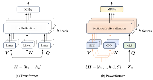
where are the representations of Query, Key, Value components in the -th layer Transformer of the -th attention head in MHA; are the corresponding parameter matrices to be learned by the model. is the total number of attention heads and is the concatenate operation. The symbol represents the transpose of matrix, and denotes the dot product operation. is the self-attention matrix of the -th head at the -th layer. Fig. 2a illustrates the traditional Transformer architecture.
3 Method
3.1 Overall Architecture
An overview of the Powerformer architecture is presented in Fig. 2b, illustrating the fundamental components crucial for obtaining robust representations in sectional power system networks, such as state factorization, Graph Neural Network (GNN) propagation, and section-adaptive attention, etc. Different from the conventional Transformer, our architecture utilizes the set as input, which consists of the state feature matrix, section power flow, and graph structure information. The section-specific information is utilized to learn Query representation, enabling the development of section-adaptive attention mechanism. To address the specific electrical factors on buses, we disentangle the system state representation into distinct factors to prevent feature coupling during propagation, and then incorporate the section-adaptive attention matrices to establish the multi-factor section-adaptive attention mechanism. Furthermore, to enhance the expressiveness of Key, Value propagation, we utilize the popular GNN architecture to embed the graph structure information into the final state representation.
3.2 Powerformer for Sectional Power System
State Factorization and GNN propagation. Each node in the power system includes important state factors, such as active power, reactive power, voltage magnitude, and phase angle, providing comprehensive insights into the state characteristic of power system.
If the state matrix is directly inputted into the propagation layer, it will result in the coupling of different factors, causing the redundancy in the learned features and ultimately diminishing the expressive power. Thus, we begin by disentangling the input state feature into factors, with the -th layer’s representation of the -th factor denoted by .
Furthermore, for the propagation of the Key and Value components in relation to the -th factor, we utilize the widely-used GNN to incorporate the power system’s graph topological structure for efficient updates:
| (5) |
where represent the GNN propagation to update the Key and Value: . Specifically, this propagation is implemented using a Graph Isomorphism Network (GIN) model [24]:
| (6) |
where represents the feature vector of node at the -th layer. refers to the neighborhood set of node based on the edge set . MLP is the Multi-layer Perceptron network.
Section-adaptive Attention (SA). For section-adaptive representations, we first utilize the power flow information of the transmission lines on the current section to encode the section, and set the power flow information that is not within the section to zero. The resulting initialization representation is . Then, we use a MLP network to learn the Query component and align its dimensions with and :
| (7) |
where is the employed MLP to update section representation. The updated Query is . Moreover, it is worth noting that the Query component in our architecture does not require the state factorization. Then, the section-adaptive attention without softmax function within the -factor can be expressed as:
| (8) |
where the achieved is the section-adaptive attention matrix of the -th factor at the -layer.
Multi-factor Section-adaptive Attention (MFSA). In order to achieve an effective representation fusion of multiple factors, it is essential to effectively integrate the weights allocated to different factors across nodes. Particularly, we recombine a new attention matrix, which is actually formed by combining different section-adaptive attention matrices, and then apply the softmax function on the dimensions of these factors:
| (9) |
| (10) |
where is the resulting matrix by applying the softmax function along the factor’s dimension. Finally, the Multi-factor Section-adaptive Attention (MFSA) mechanism:
| (11) |
where and are obtained from Eq. 5 and 9, denotes -th column associated with -th electrical factor. Symbol denotes the Hadamard product with broadcast mechanism. It is important to note that the left matrix side of the operation is in , while the right matrix is in . The resulting matrix after the Hadamard product will also reside in the space .
3.3 The Implementation of Powerformer
At the implementation stage, we merge the Eq. 8, 9 and 10 into Eq. 11 in order to provide a more clear formulation of our proposed Powerformer architecture:
| (12) |
| (13) |
| (14) |
| (15) |
where , , are the corresponding propagation function for the Query, Key and Value components. Notably, our section-adaptive attention based representation (Eq. 13) diverges from the self-attention based representation (Eq. 3) by employing softmax on the attention matrix (Eq. 14) that considers all factors, rather than the attention matrix of a single head. Furthermore, we employ the summation operation to combine diverse factor representations, rather than concatenation in MHA.
Joint Training. To deliver the final dispatch policy based on the proposed Powerformer framework, we adopt the Dueling Deep Q Network (DQN) method [14] to train a deep reinforcement learning agent. Specifically, we introduce a Q-network parameterized by , which takes the state representation as input and estimates the Q-values for each possible dispatch action . The dispatch policy with respect to is defined as , where is the dispatch action space.
During training, the agent first interacts with the environment to generate episodes using the -greedy policy based on the the current Q-network . The transition tuples encountered during training are stored in the replay buffer [25], where is the environmental reward. Then the Q-network is trained using mini-batch gradient descent on the temporal difference loss as:
| (16) |
where the tuples are sampled from the replay buffer . DQN uses the target network to make the optimization procedure more stable. The target value depend on previous network parameters but this dependency is ignored during backpropagation.
3.4 Discussions
From the Perspective of Computer Science. 1) Complexity Analysis. The time complexity of Powerformer can be analyzed based on Multi-factor Section-adaptive Attention (MFSA) and Graph Neural Network (GNN) propagation. MFSA is , where represents the number of bus nodes and represents the dimensionality of the embeddings. On the other hand, GNN propagation is , where represents the number of transmission lines. As a result, Powerformer exhibits a time complexity of , while the traditional Transformer is . 2) Difference from Traditional Transformer. According to the Fig. 2, our Powerformer adopts a Transformer based architecture to integrate the section information, which is the the main distinction from the existing architectures. This is the first attempt to use the transformer architecture in the field of transmission section power flow adjustment.
From the Perspective of Power System. In the field of transmission section power flow adjustment, the use of traditional optimal power flow (OPF) methods cannot consider the complexity of real-world scenarios. Additionally, with the expansion of the power system, OPF also raises concerns regarding real-time performance. Therefore, the deep reinforcement learning (DRL) based methods has emerged as an innovative alternative for power dispatch. Specifically, our proposed Powerformer demonstrates its effectiveness not only based on the success rate and economic benefits of the dispatch in three cases but also in terms of its fast adjustment time, which meets the demands of real-world scenarios.
4 Case Study
To demonstrate the effectiveness of our proposed Powerformer, comprehensive case studies have been conducted. In this section, we first provide the details of experimental setting. Subsequently, we conduct a comparative analysis of our method with concat and attention-based representation learning methods, as well as several popular adjustment baselines. Finally, we conduct ablation studies to enhance the understanding of our proposed method.
4.1 Experimental Setting
Scenario Generation. To obtain adequate scenarios for training and testing purposes, we first employ two small-scale systems, namely the IEEE 118-bus system and a realistic China 300-bus system. Then, we adopt a very large European 9241-bus system from the PEGASE project into our operations [26]. The detailed scenario generation is summarized as follows:
-
1.
To simulate a variety of scenarios within the power system more effectively, we implement random perturbations to loads and generators. For each scenario, we randomly select 25% of generators and loads and then introduce random disturbances to their initial power flow ranging from 10% to 200%, with intervals.
-
2.
The power range for each transmission section is pre-scheduled, as detailed in Table 1. Insecure scenarios, where the power flow of the corresponding transmission sections exceeds pre-scheduled power range, are considered for case studies during each power flow adjustment.
| Section | 118-bus System | 300-bus System | 9241-bus System | |||
| Lower | Upper | Lower | Upper | Lower | Upper | |
| 1 | 90 | 640 | 140 | 1000 | 15 | 110 |
| 2 | 50 | 360 | 280 | 1960 | 840 | 5880 |
| 3 | 40 | 290 | 170 | 1200 | 145 | 1000 |
| 4 | 90 | 640 | 240 | 1680 | 55 | 390 |
| 5 | 70 | 480 | 460 | 3200 | 560 | 3920 |
| 6 | 45 | 300 | 200 | 1400 | 360 | 2520 |
| 7 | 130 | 880 | 200 | 1400 | 345 | 2410 |
| 8 | 55 | 390 | 480 | 3360 | 760 | 5320 |
| 9 | 130 | 880 | 170 | 1200 | 130 | 910 |
| 10 | 90 | 615 | 80 | 590 | 180 | 1260 |
Finally, a total of 1829 scenarios were generated for the IEEE 118-bus system, with 1656 scenarios used for training and 173 for testing. Similarly, the China 300-bus system resulted in 1817 scenarios, including 1637 for training and 180 for testing. The European 9241-bus system produced 2037 scenarios, with 1848 for training and 189 for testing.
| Method | 118-bus System | 300-bus System | 9241-bus System | |||
|---|---|---|---|---|---|---|
| Success Rate (%) | Economic Cost ($) | Success Rate (%) | Economic Cost ($) | Success Rate (%) | Economic Cost ($) | |
| Concat | 68.44 (-28.17) | 626,215 (+4,017) | 57.66 (-37.14) | 992,048 (+22,366) | 37.57 (-5.29) | 324,485 (-2) |
| Attention | 85.23 (-11.38) | 625,128 (+2,930) | 85.30 (-9.50) | 972,573 (+2,891) | 31.13 (-11.73) | 325,152 (+665) |
| Powerformer (Ours) | 98.19 | 622,198 | 97.36 | 969,682 | 68.25 | 324,487 |
Compared Methods and Parameter Settings. We first consider two basic architectures for state representations learning on sectional power system: 1) Concat architecture. We employ a MLP network that takes the concatenated vector of the task encoding vector and state feature vector as input. 2) Attention architecture. We utilize the soft attention network [27], which allows agent to dynamically select different network modules based on the section representation. Furthermore, the proposed Powerformer is compared with several popular DRL methods, including Deep Q Network (DQN) [25], Double DQN [28], Dueling DQN [14], Advantage Actor Critic (A2C) [29], Proximal Policy Optimization (PPO) [30].
The proposed Powerformer employs a two-layer networks configuration, specifically the hidden dimension is 64. Additionally, the section encoder utilizes a two-layer MLP network with a candidate hidden dimension set {128, 64}. To implemente the Powerformer, we utilize the Before Transformer architecture [31], a type of graph transformer. The Dueling architecture includes a two-layer value network with a dimension of 128 and a one-layer advantage network with a dimension of 128. The section representation is , where 4 is the corresponding electrical factors of active power, reactive power, voltage magnitude, and phase angle, denotes the number of the transmission lines. All network modules in the architecture employ the ReLU activation function. During each training iteration, batches of 64 episodes are sampled from a replay buffer containing 20,000 episodes. The target update interval is set to 100, and the discount factor is 0.9. For exploration, we apply an epsilon-greedy approach, where epsilon linearly decreases from 0.1 to 0.01 over 500,000 training steps and remains constant thereafter.
Evaluations. The evaluation of policies incorporates metrics such as the mean test success rate, mean test economic cost, and mean inference speed across a range of tasks.
4.2 Comparison with Different State Representations
In this subsection, our primary focus revolves around a comprehensive comparison between our novel Powerformer and two commonly used representation learning methods, i.e., concat and attention-based representations. By conducting a comprehensive analysis using the same reinforcement learning framework of Dueling DQN [14], we aim to clearly showcase the remarkable effectiveness and superiority of our proposed Powerformer method.

(4-section Task)
(4-section Task)
(4-section Task)
(10-section Task)
(10-section Task)
(10-section Task)
| Method | 118-bus System (4-section Task) | 300-bus System (4-section Task) | 9241-bus System (4-section Task) | |||
|---|---|---|---|---|---|---|
| Success Rate (%) | Economic Cost ($) | Success Rate (%) | Economic Cost ($) | Success Rate (%) | Economic Cost ($) | |
| DQN | 88.97 (-19.66) | 693,272 (+1,130) | 79.05 (-20.68) | 981,695 (+19,605) | 52.04 (-16.93) | 325,331 (-99) |
| Double DQN | 87.63 (-12.04) | 693,653 (+1,511) | 80.15 (-19.58) | 995,038 (+32,948) | 55.41 (-13.56) | 325,464 (+34) |
| Dueling DQN | 91.17 (-8.50) | 692,378 (+236) | 71.45 (-28.28) | 995,279 (+33,189) | 52.48 (-16.49) | 325,266 (-164) |
| A2C | 84.98 (-14.69) | 697,853 (+5,711) | 93.71 (-6.02) | 974,455 (+12,365) | 53.07 (-15.90) | 325,093 (-337) |
| PPO | 26.67 (-73.00) | 673,399 (-18,743) | 46.88 (-52.85) | 937,454 (-24,636) | 39.18 (-29.79) | 326,614 (+1,184) |
| OPF | 83.33 (-16.34) | 639,782 (-52,360) | 56.78 (-42.59) | 956,120 (-5,970) | 64.47 (-4.50) | 324,995 (-435) |
| Powerformer (Ours) | 99.67 | 692,142 | 99.73 | 962,090 | 68.97 | 325,430 |
| Method | 118-bus System (10-section Task) | 300-bus System (10-section Task) | 9241-bus System (10-section Task) | |||
| Success Rate (%) | Economic Cost ($) | Success Rate (%) | Economic Cost ($) | Success Rate (%) | Economic Cost ($) | |
| DQN | 61.23 (-35.38) | 626,808 (+4,610) | 56.74 (-38.06) | 991,762 (+22,080) | 13.67 (-29.19) | 324,658 (+164) |
| Double DQN | 53.28 (-43.33) | 638,079 (+15,881) | 61.24 (-33.49) | 990,126 (+20,444) | 16.75 (-26.11) | 324,792 (+305) |
| Dueling DQN | 68.44 (-28.17) | 626,215 (+4,017) | 57.66 (-37.14) | 992,048 (+22,366) | 37.57 (-5.29) | 324,485 (-2) |
| A2C | 80.14 (-16.47) | 626,703 (+4,505) | 75.61 (-19.19) | 976,467 (+6,785) | 12.70 (-30.16) | 325,000 (+513) |
| PPO | 24.28 (-72.33) | 596,315 (-25,883) | 48.61 (-46.19) | 930,581 (-39,101) | 19.40 (-23.46) | 325,549 (+1,062) |
| OPF | 72.25 (-24.36) | 606,259 (-15,939) | 50.56 (-44.24) | 953,349 (-16,333) | 51.32 (+8.46) | 321,586 (-2,901) |
| Powerformer (Ours) | 98.19 | 622,198 | 97.36 | 969,682 | 68.25 | 324,487 |
The performance results presented in Table 2 showcases a comparison between the Powerformer and two fundamental state encoding methods—Concat and Attention—across three different power system cases. The adopt evaluation is based on two metrics: success rate and economic cost, averaged over five trials. Among these results, it is worth noting that the proposed Powerformer demonstrates the exceptional success rates of 98.19%, 97.36%, and 68.25% respectively, solidifying its position as the standout performer. This is particularly evident in its remarkable performance when applied to large-scale power systems such as the European 9241-bus system. In terms of economic cost, Powerformer tends to be more efficient or on par with the other methods. This suggests that Powerformer can achieve higher performance without a relatively low test economic cost, an important consideration for practical applications.
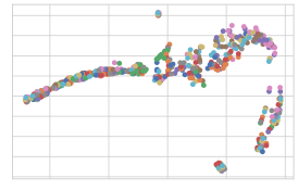
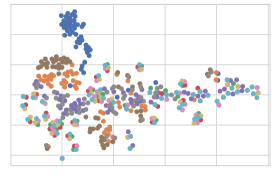
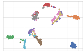
Furthermore, we utilize the t-SNE toolkit to visually illustrate the distribution of state representations for 10 distinct section tasks on the IEEE 118-bus system in Fig. 3. Our proposed Powerformer approach can effectively cluster 10 different section tasks into 10 distinct central points, while the other two methods cannot accomplish. This also explains the poor performance of the other two state encoding methods, as they couple the transmission section representation and different electrical factors of node features together (Fig. 3a and 3b), making it impossible to execute specific actions.
4.3 Comparison with Different Adjustment Baselines
To demonstrate the superiority of our method in efficiently and effectively adjusting transmission section power flow, we thoroughly analyze and compare our method with various popular approaches in deep reinforcement learning (DRL) framework, as well as a well-established traditional optimal power flow (OPF) adjustment method. Moreover, in order to thoroughly validate the effectiveness of our Powerformer, we design the additional 4-section power flow adjustment tasks, which aims to deal with the top four ranked sections in terms of transmission capacity among a total of ten sections.
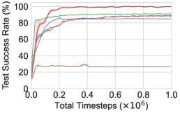
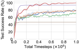
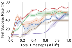
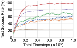
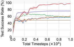
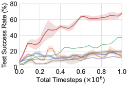
Through analyzing the learning curve in Fig. 4, our proposed method has successfully achieved the best test success rate among all considered architectures on three different systems. Although DQN and its variants require fewer timesteps to achieve reasonable results, Dueling DQN stands out with the highest achieved test success. This also provides advantageous conditions for our method to obtain the best results. We can analyze and compare the superiority of our method based on the difficulty levels of different tasks, especially in the more challenging task of 10-section adjustment (i.e., Fig. 4d, 4e and 4f), where the effectiveness of our method is highlighted. Furthermore, from the perspective of different system cases, our method performs even better on large-scale datasets. This is because our method is able to learn better representations of sectional power system states, thus avoiding the coupling of state features. We can comparatively analyze the learning curve on the IEEE 118-bus and European 9241-bus systems, and the significant differences in the effectiveness of our method can be directly observed because when the system case is simple, the task is also relatively simple, hence the superiority is not so apparent.
From a quantifiable perspective of comparison adjustment algorithms, we leverage the comparative results of success rates and economic costs pertaining to 4-section and 10-section adjustment tasks, as evidenced in Table 3, to serve as prime examples for our comprehensive analysis. Specifically, we further analyze the results by examining different power system cases. For the IEEE 118-bus system, Powerformer outperforms all other methods with a success rate of 99.67%, significantly surpassing Dueling DQN (91.17%) on the 4-section task. As complexity increases in the 10-section task, Powerformer maintains a success rate of 98.19%, outperforming A2C (80.14%) by a substantial margin. For the China 300-bus system, Powerformer continues to exhibit a satisfying level of performance in comparison to the baseline approaches, accomplishing an impressively high test success rate of and on the 4-section and 10-section tasks, respectively. For the European-9241 system, our method consistently demonstrates exceptional performance, achieving an impressive success rate of 68.97% and 68.25% when considering the test success rates of 4-section and 10-section tasks. In contrast, alternative reinforcement learning methods fail to surpass the 35% threshold for the complex 10-section task. Additionally, our method consistently demonstrates its exceptional ability to achieve relatively low economic costs across all scenarios.

| 118-bus System | 300-bus System | 9241-bus System | |
|---|---|---|---|
| OPF | 44.822 38.459 | 47.668 28.230 | 1912.608 1636.746 |
| Powerformer (Ours) | 0.078 0.151 | 0.121 0.176 | 0.585 0.602 |
4.4 Inference Time Analysis
In real-time applications, such as the European 9241-bus system, inference time plays a critical role, particularly in large-scale systems. In such scenarios, power flow adjustment becomes more complex due to the numerous variations that need careful consideration and strategic decision-making. To better understand the superiority of our method in terms of inference speed, we provide Fig. 5 and Table 4 to demonstrate the advantages of our approach when compared to traditional OPF method used in practical scenarios. As shown in Fig. 5, the experimental results demonstrate that, when compared to the traditional OPF method, the time required to successfully achieve the predefined range for each individual test is significantly reduced across a comprehensive set of 173 test scenarios in the IEEE 118-bus system. Moreover, it is notable that our method exhibits a noteworthy reduction in inference time across three different power systems, as evidenced by the compelling numerical statistics presented in Table 4. As a result, our proposed method is remarkably more time efficient than the traditional OPF approach, especially as the system size increases, making the OPF method impractical.


4.5 Visualization Analysis
To better understand the superiority of the proposed Powerformer, we present illustrations that depict active power and economic cost across the 10 transmission sections.
Active Power Comparison. By comparing the active power of all scenario samples before and after Powerformer adjustment, across all ten transmission sections on the IEEE 118-bus system, we can find that all test samples are successfully adjusted into the pre-determined range. Among these cases shown in Fig. 7, the majority involve adjusting the situation where the power flow exceeds the limit to align with the range of the upper bound, thereby guaranteeing the safe operation of the power system and ensuring its long-term stability.
Economic Cost Comparison. By comparing the economic cost of all scenario samples before and after Powerformer adjustment on all ten transmission sections of the IEEE 118-bus system, we can find that the economic cost of all test samples has been reduced. As shown in Fig. 7, after undergoing further adjustment through Powerformer, the economic cost of nearly every sample has been effectively reduced, with no instances of cost increase. Hence, it can be inferred that our method reliably aims to reduce economic cost.
4.6 Ablation Study
By conducting thorough ablation studies and performing a detailed analysis, we go deeper insights into our proposed Powerformer (PF) architecture. We carefully assess and quantify the contributions of each component, revealing how they individually impact the overall effectiveness and superiority of the algorithm. Fig. 8 presents the comparison results obtained from an array of ablation experiments conducted on IEEE 118-bus system with 10-section task. These research findings provide valuable insights, clarifying the roles of each component in improving performance.
Powerformer-E (PF-E). This method only employs GNN to learn state representation, without performing state factorization operation and integrating transmission section information. This method lacks specific feature extraction for individual electrical factors, resulting in the coupling of features. Moreover, the absence of section information undermines the accuracy of the representation vector in depicting the current system state, thereby impeding effective decision-making.
Powerformer-S (PF-S). This method only utilizes the representation of Value component (Fig. 2) as the final representation of the system state. In contrast to Powerformer-E, it involves the addition of an additional factorization operation. By analyzing the results in Fig. 8, it is evident that comparing Powerformer-S with Powerformer highlights the inadequacy of relying solely on state representations. This emphasizes the importance of incorporating section information.
Powerformer-M (PF-M). This method skips the factorization operation and use the raw four-dimensional electrical features as input to learn the final representation within the Powerformer architecture. In contrast to Powerformer-E, it incorporates an additional operation for combining the transmission section information. The less satisfactory result in Fig. 8 implies that the disentangling operation plays a crucial role in determining the final performance.
5 Conclusion
In this paper, we propose and present a specialized Transformer architecture, named Powerformer, which integrates the transmission section power flow information in order to address the issue of power flow adjustment. The utilization of our proposed architecture facilitates controlled power dispatch, leading to improved stability of the power system. Specifically, our proposed Powerformer incorporates transmission section information into the existing Transformer and develops a section-adaptive attention mechanism. Furthermore, our approach disentangles power system graph data into independent electrical factor graphs to conduct a multi-factor attention mechanism, and employs graph neural networks to extract system state features while considering the graph topological structure of the power system. This allows for the robust representations of the sectional power system state, enabling the development of efficient strategies to effectively manage and adjust transmission section power flow. In our future work, we will focus on developing more efficient architectures for factorization and attribution to enhance the performance in adjusting transmission section power flow.
References
- [1] L. Min, A. Abur, Total transfer capability computation for multi-area power systems, IEEE Transactions on power systems 21 (3) (2006) 1141–1147.
- [2] J.-H. Liu, C.-C. Chu, Iterative distributed algorithms for real-time available transfer capability assessment of multiarea power systems, IEEE Transactions on Smart Grid 6 (5) (2015) 2569–2578.
- [3] Y. Jiang, Z. Ren, X. Yang, Q. Li, Y. Xu, A steady-state energy flow analysis method for integrated natural gas and power systems based on topology decoupling, Applied Energy 306 (2022) 118007.
- [4] F. Capitanescu, J. M. Ramos, P. Panciatici, D. Kirschen, A. M. Marcolini, L. Platbrood, L. Wehenkel, State-of-the-art, challenges, and future trends in security constrained optimal power flow, Electric power systems research 81 (8) (2011) 1731–1741.
- [5] S. Dutta, S. Singh, Optimal rescheduling of generators for congestion management based on particle swarm optimization, IEEE transactions on Power Systems 23 (4) (2008) 1560–1569.
- [6] Y. Li, C. Yu, M. Shahidehpour, T. Yang, Z. Zeng, T. Chai, Deep reinforcement learning for smart grid operations: Algorithms, applications, and prospects, Proceedings of the IEEE (2023).
- [7] M. Wang, M. Feng, W. Zhou, H. Li, Stabilizing voltage in power distribution networks via multi-agent reinforcement learning with transformer, in: Proceedings of the 28th ACM SIGKDD Conference on Knowledge Discovery and Data Mining (KDD), 2022, pp. 1899–1909.
- [8] A. Vaswani, N. Shazeer, N. Parmar, J. Uszkoreit, L. Jones, A. N. Gomez, Ł. Kaiser, I. Polosukhin, Attention is all you need, in: Neural Information Processing Systems (NeurIPS), 2017, pp. 6000–6010.
- [9] W. Zhu, T. Wen, G. Song, L. Wang, B. Zheng, On structural expressive power of graph transformers, in: Proceedings of the 29th ACM SIGKDD Conference on Knowledge Discovery and Data Mining (KDD), 2023, pp. 3628–3637.
- [10] H. Zhang, J. Duan, M. Xue, J. Song, L. Sun, M. Song, Bootstrapping vits: Towards liberating vision transformers from pre-training, in: Proceedings of the IEEE/CVF Conference on Computer Vision and Pattern Recognition, 2022, pp. 8944–8953.
- [11] Y. Jing, Efficient representation learning with graph neural networks, Ph.D. thesis (2023).
- [12] W. Li, K. Chen, S. Liu, W. Huang, H. Zhang, Y. Tian, Y. Su, M. Song, Message-passing selection: Towards interpretable gnns for graph classification, in: Tiny Track @ International Conference on Learning Representations (ICLR), 2023.
- [13] J. Zhang, D. Luo, H. Wei, Mixupexplainer: Generalizing explanations for graph neural networks with data augmentation, in: Proceedings of the 29th ACM SIGKDD Conference on Knowledge Discovery and Data Mining (KDD), 2023, pp. 3286–3296.
- [14] Z. Wang, T. Schaul, M. Hessel, H. Hasselt, M. Lanctot, N. Freitas, Dueling network architectures for deep reinforcement learning, in: International Conference on Machine Learning (ICML), 2016, pp. 1995–2003.
- [15] S. Liu, W. Luo, Y. Zhou, K. Chen, Q. Zhang, H. Xu, Q. Guo, M. Song, Transmission interface power flow adjustment: A deep reinforcement learning approach based on multi-task attribution map, IEEE Transactions on Power System (2023).
- [16] Y. Zhang, Q. Yang, An overview of multi-task learning, National Science Review 5 (1) (2018) 30–43.
- [17] M. Tan, C. Liao, J. Chen, Y. Cao, R. Wang, Y. Su, A multi-task learning method for multi-energy load forecasting based on synthesis correlation analysis and load participation factor, Applied Energy 343 (2023) 121177.
- [18] K.-X. Chen, J.-Y. Ren, X.-J. Wu, J. Kittler, Covariance descriptors on a gaussian manifold and their application to image set classification, Pattern Recognition 107 (2020) 107463.
- [19] Z. Chen, T. Xu, X. Wu, R. Wang, Z. Huang, J. Kittler, Riemannian local mechanism for spd neural networks, in: Proceedings of the AAAI Conference on Artificial Intelligence (AAAI), 2023, pp. 7104–7112.
- [20] Z. Chen, T. Xu, X.-J. Wu, R. Wang, J. Kittler, Hybrid riemannian graph-embedding metric learning for image set classification, IEEE Transactions on Big Data 9 (01) (2023) 75–92.
- [21] L. Sun, T. Liu, D. Wang, C. Huang, Y. Xie, Deep learning method based on graph neural network for performance prediction of supercritical co2 power systems, Applied Energy 324 (2022) 119739.
- [22] Z. Chen, W. Zhang, Y. Huang, M. Chen, Y. Geng, H. Yu, Z. Bi, Y. Zhang, Z. Yao, W. Song, X. Wu, Y. Yang, M. Chen, Z. Lian, Y. Li, L. Cheng, H. Chen, Tele-knowledge pre-training for fault analysis, in: International Conference on Data Engineering (ICDE), 2023, pp. 3453–3466.
- [23] K. Chen, S. Liu, T. Zhu, J. Qiao, Y. Su, Y. Tian, T. Zheng, H. Zhang, Z. Feng, J. Ye, et al., Improving expressivity of gnns with subgraph-specific factor embedded normalization, in: Proceedings of the 29th ACM SIGKDD Conference on Knowledge Discovery and Data Mining (KDD), 2023, pp. 237–249.
- [24] K. Xu, W. Hu, J. Leskovec, S. Jegelka, How powerful are graph neural networks?, in: International Conference on Learning Representations (ICLR), 2019.
- [25] V. Mnih, K. Kavukcuoglu, D. Silver, A. A. Rusu, J. Veness, M. G. Bellemare, A. Graves, M. A. Riedmiller, A. K. Fidjeland, et al., Human-level control through deep reinforcement learning, Nature 518 (7540) (2015) 529–533.
- [26] C. Josz, S. Fliscounakis, J. Maeght, P. Panciatici, Ac power flow data in matpower and qcqp format: itesla, rte snapshots, and pegase, arXiv preprint arXiv:1603.01533 (2016).
- [27] R. Yang, H. Xu, Y. Wu, X. Wang, Multi-task reinforcement learning with soft modularization, in: Neural Information Processing Systems (NeurIPS), 2020, pp. 4767–4777.
- [28] H. V. Hasselt, A. Guez, D. Silver, Deep reinforcement learning with double q-learning, in: Proceedings of the AAAI Conference on Artificial Intelligence (AAAI), 2016, pp. 2094–2100.
- [29] V. Mnih, A. P. Badia, M. Mirza, A. Graves, T. P. Lillicrap, T. Harley, D. Silver, K. Kavukcuoglu, Asynchronous methods for deep reinforcement learning, in: International Conference on Machine Learning (ICML), 2016, pp. 1928–1937.
- [30] J. Schulman, F. Wolski, P. Dhariwal, A. Radford, O. Klimov, Proximal policy optimization algorithms, arXiv preprint arXiv:1707.06347 (2017).
- [31] E. Min, R. Chen, Y. Bian, T. Xu, K. Zhao, W. Huang, P. Zhao, J. Huang, S. Ananiadou, Y. Rong, Transformer for graphs: An overview from architecture perspective, arXiv preprint arXiv:2202.08455 (2022).