A Cost-Efficient FPGA Implementation of Tiny Transformer Model using Neural ODE
Abstract
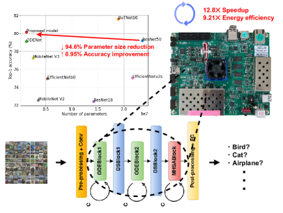
Transformer is an emerging neural network model with attention mechanism. It has been adopted to various tasks and achieved a favorable accuracy compared to CNNs and RNNs. While the attention mechanism is recognized as a general-purpose component, many of the Transformer models require a significant number of parameters compared to the CNN-based ones. To mitigate the computational complexity, recently, a hybrid approach has been proposed, which uses ResNet as a backbone architecture and replaces a part of its convolution layers with an MHSA (Multi-Head Self-Attention) mechanism. In this paper, we significantly reduce the parameter size of such models by using Neural ODE (Ordinary Differential Equation) as a backbone architecture instead of ResNet. The proposed hybrid model reduces the parameter size by 94.6% compared to the CNN-based ones without degrading the accuracy. We then deploy the proposed model on a modest-sized FPGA device for edge computing. To further reduce FPGA resource utilization, we quantize the model following QAT (Quantization Aware Training) scheme instead of PTQ (Post Training Quantization) to suppress the accuracy loss. As a result, an extremely lightweight Transformer-based model can be implemented on resource-limited FPGAs. The weights of the feature extraction network are stored on-chip to minimize the memory transfer overhead, allowing faster inference. By eliminating the overhead of memory transfers, inference can be executed seamlessly, leading to accelerated inference. The proposed FPGA implementation achieves 12.8 speedup and 9.21 energy efficiency compared to ARM Cortex-A53 CPU.
1 Introduction
Transformer-based [1] model with a sophisticated attention mechanism has been an active research topic. ViT (Vision Transformer) [2] is the first pure Transformer-based architecture for visual tasks and achieves promising results compared to existing CNN-based models. However, training such models require large-scale datasets, e.g., JFT-300M [3], limiting the application on resource-limited platforms. Generally, this is due to the lack of inductive biases (e.g., locality and translational invariance) in the attention mechanism. Thus, one of the solutions for alleviating the dependence on large datasets is to combine both convolution and attention mechanism [4, 5, 6, 7, 8, 9]. Such hybrid models can achieve the state-of-the-art accuracy for small- or medium-scale datasets in a variety of tasks.
Among these models, we focus on BoTNet (Bottleneck Transformer Network) [7], which replaces spatial convolutions in the last three bottleneck blocks in ResNet with the global self-attention and outperforms baseline models by a large margin. It achieves 84.7% top-1 accuracy on ImageNet benchmark.
Based on the growing number of IoT devices, the demand for deploying DNNs to edge devices (e.g., self-driving cars, security cameras, and drones) has increased. FPGA is becoming an attractive platform to accelerate DNNs due to its energy efficiency, reconfigurability, and short development period. We aim to implement the proposed model on a modest-sized FPGA such as Xilinx ZCU104. In our previous work [10], an MHSA mechanism was implemented on the FPGA; since a large part of the model was still performed on the host CPU, only a moderate performance improvement was achieved. In contrast, this paper implements the entire feature extraction network of the proposed model on the FPGA to fully harness its computational capability. Additionally, to reduce FPGA resources, in this paper we choose to employ a lightweight quantization technique by considering the characteristics of Neural ODE. The parameter reduction and model quantization play an important role to save the scarce on-chip memory and map the Transformer-based model onto such FPGAs.
In this paper, we propose a tiny Transformer-based model (see Fig. 1) for resource-constrained edge devices by approximating the ResNet computation with Neural ODE [11], which reformulates the forward propagation of ResNet blocks as a numerical solution of ODEs. The number of parameters is greatly reduced because the forward pass through multiple ResNet building blocks is replaced by an iteration of the same single block, as shown in Fig. 1 (bottom).
The rest of this paper is organized as follows. Sec. 2 presents related works and compares our work with them. Sec. 3 provides the background on MHSA mechanism, Neural ODE, and quantization. Sec. 4 presents the design of the proposed Transformer-based lightweight model by using Neural ODE. Sec. 5 implements the proposed model on the FPGA board using quantization technique to accelerate the inference speed. Sec. 6 shows evaluation results of the proposed model in terms of parameter size and accuracy and those of the FPGA implementation in terms of resource utilization, execution time, and energy efficiency. Sec. 7 concludes this paper and discusses our future work.
2 Related work
2.1 CNN and Transformer
In recent years, numerous Transformer-based models have been proposed for image recognition tasks. ViT [2] is a pure Transformer-based model for image recognition and achieves greater accuracy than CNN-based models with a large dataset (e.g., JFT-300M). However, one major drawback of ViT is that it performs worse than CNN-based models when trained with small- to medium-scale datasets such as CIFAR-10/100 [12] and ImageNet [13] due to the lack of intrinsic inductive biases.
CNNs have strong inductive biases such as spatial locality and translational invariance. The spatial locality is an assumption that each pixel only correlates to its spatially neighboring pixels. While this assumption allows to efficiently capture local structures in image recognition tasks, it also comes with a potential issue of lower performance bound. On the other hand, an attention mechanism omits such inductive biases and aims to capture global structures. In this case, the model has to be trained with large datasets to capture the important relationships between different parts of each input image, which may or may not be spatially close to each other.
Therefore, hybrid models that combine MHSA and convolution have been proposed [4, 5, 6, 7, 8, 9]. BoTNet [7] is introduced as a simple modification to ResNet, which replaces a part of convolutions with MHSAs, and has shown an improved accuracy in object detection, instance segmentation, and image classification. The experimental results in [7] show accuracy improvements with larger image size and scale jitter, demonstrating the benefits of including MHSA blocks in the model. By analyzing the relationship between convolution and MHSA, it is shown that CNN tends to increase the dispersion of feature maps while MHSA tends to decrease it [8]. Considering these characteristics, AlterNet [8] is proposed to suppress the dispersion of feature maps by adding MHSA to the final layer of each stage in ResNet. It is shown that MHSA contributes to an improved accuracy and a flat and smooth loss surface, thereby increasing the model’s robustness; as a result, AlterNet outperforms existing models on small datasets.
Many attention variants have been proposed to address the high computational cost of MHSA, which grows with the square of input size . In Reformer [14], LSH (Locality Sensitive Hashing) technique is employed to efficiently retain regions with high attention scores, thereby reducing the computation complexity from to . Other methods propose the Transformer with linear complexity . In linear Transformer [15], the softmax operator is decomposed into two terms by employing a kernel method. Linformer [16] is a low-rank factorization-based method. Furthermore, in Flash Attention [17], memory-bound Transformer processing is accelerated by introducing an IO-aware algorithm on GPUs. These methods are proposed to overcome the computation cost associated with lengthy texts for NLP (Natural Language Processing) tasks. A similar challenge arises in the context of high-resolution image recognition tasks. Swim Transformer [18] employs fixed-pattern and global memory-based methods to reduce the computation cost from to .
2.2 Reduction of model computational complexity
Considering the application of AI models on edge devices, running the inference of large-scale networks on such devices is intractable due to resource limitations. Generally, various techniques such as pruning, quantization, and low-rank factorization are employed for model compression. Aside from these, Neural ODE [11] can be applied to ResNet-family of networks with skip connections to reduce the number of parameters while avoiding the accuracy loss. It is emerging as an attractive approach to tackle the high computational complexity of large networks. Specifically, Neural ODE formulates the propagation of ResNet as ODE systems, and the number of parameters is reduced by turning a set of building blocks into multiple iterations of a single block, i.e., reusing the same parameters.
Several extensions to Neural ODE have been proposed in the literature. Neural SDE (Stochastic Differential Equation) [19] incorporates various common regularization mechanisms based on the introduction of random noise. This model shows greater robustness to input noise, whether they are intentionally adversarial or not, compared to Neural ODE. In [20], training cost is significantly reduced without sacrificing accuracy by applying two appropriate regularizations to Neural ODE. In [21], by considering the regularization, TisODE (Time-invariant steady Neural ODE) is proposed to further enhance the robustness of vanilla Neural ODE. In [22], inherent constraints in Neural ODE are identified, and more expressive model called ANODE (Augmented Neural ODE) is proposed. These approaches are crucial in achieving robustness, approximation capabilities, and performance improvements in the context of Neural ODE. While this paper incorporates Transformer architecture into a model with vanilla Neural ODE as a backbone, the same idea can be applied to these Neural ODE extensions as well, which is not the focus of this paper. To further enhance our proposed model performance, we can incorporate the above techniques as future work.
2.3 FPGA implementation of Transformer architecture
There is ongoing research on FPGA implementation of Transformer to improve the inference speed. In [23], an FPGA acceleration engine that employs a column balanced block-wise pruning is introduced for customizing the balanced block-wise matrix multiplications. FTRANS [24] uses a cyclic matrix-based weight representation for Transformer model for NLP. VAQF [25] proposes an automated method to implement a quantized ViT on Xilinx ZCU102 FPGA board that meets a target accuracy. Compared to our proposal, these works do not utilize CNNs (i.e., using pure Transformer models) and thus suffer from the drawbacks of attention mechanism (e.g., huge training cost). In addition, they consider the acceleration of large-scale Transformer models (e.g., ViT) for NLP tasks, which often require high-end FPGAs due to the large number of parameters. We instead present a tiny Transformer model with less than one million parameters that fits within a modest-sized FPGA (e.g., ZCU104) for image classification tasks. The parameters are stored on-chip to eliminate the memory transfer overhead, allowing efficient inference.
In [10], a lightweight Transformer model with Neural ODE is proposed along with its FPGA-based design. Since only an MHSA block is accelerated and the other part including Neural ODE blocks is still executed on a host CPU, the design shows only a limited performance gain. Contrary to that, in this paper, we implement the entire feature extraction network to further improve the inference speed and fully benefit from the computing power of FPGAs. Additionally, in [10], the model is quantized by simply converting inputs/outputs and weights from floating- to fixed-point representation. However, it is shown that performing such simple type conversions throughout the entire model would result in a significant degradation of accuracy [10]. In this paper, we instead employ QAT, which allows more aggressive bit-width reduction (e.g., 4-bit quantization) to save the on-chip memory while mitigating the risk of significant accuracy loss.
3 Preliminaries
3.1 MHSA
3.1.1 Attention mechanism
The attention mechanism aims to capture a relationship between a set of queries and a feature map to identify the region of interest in for each query , where and denote the number of elements and the number of channels for each element, respectively.
Given a query vector , its corresponding attention weight is calculated as follows:
| (1) |
An attention represents the relevance between the query and the feature element . By stacking Eq. (1), attentions for queries can be calculated in the form of matrix operation as follows:
| (2) |
Note that the softmax operator in Eq. (2) is applied row-wise to
3.1.2 Self-attention
Self-attention is a special case of the attention mechanism, where an input query is a feature map itself. It can learn how to generate better feature maps, by calculating a correlation between every pair of feature elements. First, query, key, and value matrices , , and are computed from using three learnable weights and as follows:
| (3) |
| (4) |
| (5) |
An attention map is computed by multiplying with similar to Eq. (2), namely:
| (6) |
For each query , its output is obtained by calculating the sum of values weighted by their attention scores (i.e., coefficients of the -th row vector of ) That is, the output of self-attention is calculated by taking an inner product between and as follows:
| (7) |
Unlike convolution operations, which only use a subset of input features (i.e., a local region of input features) to compute each output element, in the self-attention, all input elements will contribute to the output for each query . The self-attention thus aggregates the input feature globally and is not affected by inductive biases.
3.1.3 Positional encoding
Since the self-attention (Eq. (7)) is a set operation and is invariant to the random permutation of inputs, it causes a loss of the positional information. For example, in Eq. (2), if and are swapped, then their corresponding output elements, i.e., and , are simply swapped. The model with this property, called equivariance, is not appropriate for structural data such as images, since the model should be aware of the spatial relation of the pixels. To address this information loss, a positional encoding is often employed with the attention mechanism. A position-specific vector is added to the -th input via addition or concatenation . The positional encoding is modeled as a deterministic function with a set of fixed hyperparameters or as a learnable function. In addition, either absolute or relative position encoding can be used. Typically, Transformer [1] adopts the sinusoidal function, which is categorized as a fixed absolute encoding and is written as follows:
| (10) |
where . On the other hand, several studies [2, 18] propose to learn the relative positional encoding via MLP. In [7], the authors show that the relative position leads to better accuracy than the absolute one. Our method thus uses a learnable relative encoding.
3.1.4 MHSA
MHSA is an extension of the self-attention mechanism [1], which is comprised of multiple self-attention heads to jointly learn different relationships between features. First, each weight matrix and is partitioned column-wise into submatrices (i.e., = ), each of which is fed to a separate self-attention head. Let () be the -th self-attention head, and its output is calculated as follows:
| (11) |
where , , and . Following this, the output of MHSA is represented by Eq. (12). While the output dimension of each head is arbitrary, it is usually set to such that all heads and weight submatrices are equal-sized.
| (12) |
3.2 Neural Ordinary Differential Equation (Neural ODE)
ResNet is a widely used backbone architecture especially for image classification tasks; it introduces residual connections between CNN-based building blocks (ResBlocks) to address the vanishing gradient problem and allow training deeper networks with tens of layers. Neural ODE [11] is considered as a continuous generalization of ResNet, which interprets the skip connection as a discrete approximation of the ODE. Let denote the -th ResBlock with an input and parameters . The forward propagation of ResBlocks is formally written as recurrent updates of the hidden state as follows:
| (13) |
where the first additive term corresponds to the skip connection.
By treating the layer index as a time point and as a time-dependent parameter evaluated at , in the limit of infinitely many blocks (i.e., and ), Eq. (13) turns into an ODE with respect to as follows:
| (14) |
The solution at some time point is obtained by integrating Eq. (14):
| (15) | |||||
| (16) |
where is an initial state (i.e., input to the ResBlock) and is an arbitrary ODE solver such as Euler and Runge-Kutta methods. In the Euler method, the time is again discretized by with a small step , and is iteratively solved as follows:
| (17) |
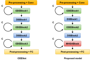
The observation of Eqs. (13) and (17) reveals that the forward propagation of a single ResBlock amounts to one iteration of the Euler method, i.e., by exploiting the Neural ODE formulation, different ResBlocks can be merged into one block (ODEBlock) that computes Eq. (17) times as shown in Fig. 2 (left). As apparent in Eq. (13), ResBlocks require individual sets of parameters ; compared to that, an ODEBlock reuses the same parameters during the iterations, leading to the -fold reduction of parameter size. Neural ODE approach allows to effectively build a compressed and lightweight alternative of ResNet-based deep models, by replacing ResBlocks with ODEBlocks. Similar to ResNets, models composed by a stack of ODEBlocks are referred to as ODENets in this paper.
3.3 Quantization of the proposed model
While there are a number of quantization methods, we employ a method based on a learnable lookup table (LLT) [26], considering its simplicity and low computational overhead. LLT-based quantization is outlined in the following.
In LLT, weight parameters and activations (i.e., layer inputs) are quantized, which are here denoted as and . Note that weights and activations have different value ranges: and . The latter is always positive because it is an output of the ReLU. Considering this, we scale and clip and to the ranges and , respectively, using the function as follows:
| (18) | |||||
| (19) |
where and are learnable scaling parameters. Using and obtained from the above equations, the quantized weight and activation are derived as follows:
| (20) | |||||
| (21) |
where and are the numbers of possible values for and , respectively. In the case of -bit quantization, and are satisfied. Furthermore, and are the mapping functions from full-precision values (i.e., and ) to -bit integers, which are realized by learnable LUTs (Look-Up Tables).
In the following, we describe the quantization process for activations. Note that weights can be quantized in the same way. The full-precision activation is converted to its nearest discrete value , which is represented by a total of learnable step functions. Here, when is within the range , it is mapped to either or by the -th step function () as follows:
| (24) |
where is a learnable threshold associated with each step function. takes one of values in , where is referred to as granularity. This function can be represented as an equivalent LUT with elements, where the first elements are and the rest are . Such LUTs are concatenated into a single integrated LUT of size , which is denoted as “I-LUT” in this paper. The quantization process with I-LUT corresponds to the function in Eq. (21). Specifically, this quantization is achieved by a simple lookup operation as follows. For an input , its corresponding index is obtained by multiplying the table size and then rounding to the nearest integer as in Eq. (25).
| (25) | |||||
| (26) |
4 Design of the proposed model
This section describes the design of the proposed model. Specifically, we outline key design aspects of the proposed model as follows: We (1) first review the ResNet architecture and (2) introduce ODENet as a memory-efficient alternative to ResNet. We then (3) apply the DSC (Depth-wise Separable Convolution) to ODENet to further reduce parameters. Analogous to BoTNet, we (4) incorporate MHSA into ODENet to derive a hybrid architecture, and (5) apply the three modifications to MHSA to make it more hardware-friendly while preserving the accuracy.
(1) ResNet consists of pre-processing, post-processing, and multiple stages for feature extraction. Pre-processing converts input images into feature maps, and post-processing transforms feature maps into a vector with elements equal to the number of classes. Each stage comprises several ResBlocks with the same structure. Specifically, each ResBlock contains two sets of convolution (Conv) layer, batch normalization (BatchNorm) layer, and activation function (e.g., ReLU), which are cascaded sequentially. In each stage, the first ResBlock is employed for downsampling, denoted as “DS”, followed by a stack of standard ResBlocks. The ResBlock for DS halves the width and height of a feature map while doubling the number of channels, i.e., it takes the feature map of size as input and produces an output of size . Note that the ResBlock for DS and standard ResBlock only differ in the configuration of the first convolution layer. For example, a straightforward approach to achieve DS is to set the stride and output channels of the first convolution in the block to 2 and , respectively.
(2) As seen in Eq. (13), the size of feature map () should remain the same during the forward propagation of ResBlocks, in order to merge them into a single ODEBlock. Since the first convolution in each stage changes the feature map size, a single ODEBlock cannot represent all ResBlocks in ResNet. Thus, we introduce special ODEBlocks corresponding to the ResBlocks for DS, referred to as DSBlocks. Based on the above, a baseline architecture of ODENet [27] is shown in Fig. 2 (left), which consists of three ODEBlocks and two DSBlocks The computation of each ODEBlock is repeated times, while each DSBlock is executed only once during inference; ODENet can be viewed as a deep network with 3 + 2 blocks in total except that ODEBlocks in the same stage reuse the same parameters. That is, ODENet in Fig. 2 (left) can be regarded as an approximation of ResNet, which consists of three stages with each having ResBlocks.
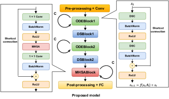
(3) Instead of the standard convolution, the lightweight CNN-based models [28, 29] employ DSC, which performs convolution in the spatial and channel dimensions separately. While the standard convolution uses a total of parameters, DSC only uses parameters, where and denote the number of input channels, the number of output channels, and kernel size, respectively. Assuming , DSC achieves approximately times parameter size reduction. As shown in Fig. 3, our model also employs DSC in the ODEBlocks.
(4) The key idea of BoTNet is to replace 33 convolutions in the last three ResBlocks with MHSA, referred to as MHSABlocks. By applying such simple modifications, BoTNet has achieved a better accuracy than ResNet on ImageNet benchmark while at the same time reducing the parameter size [7]. Since Neural ODE is a ResNet-like model, the idea of BoTNet can be applied to Neural ODE as well. As depicted in Fig. 2 (right), the final ODEBlock is replaced with MHSABlock, which has the same structure as in BoTNet. While the model can adapt to arbitrary input image sizes by only modifying the pre-processing part (Fig. 2, top), in our FPGA implementation, we assume the input image size of pixels. As shown in Table 2, it achieves 94.6 parameter size reduction compared to ResNet50, making it a tiny-sized Transformer model which is well-suited to deployment on resource-limited devices.
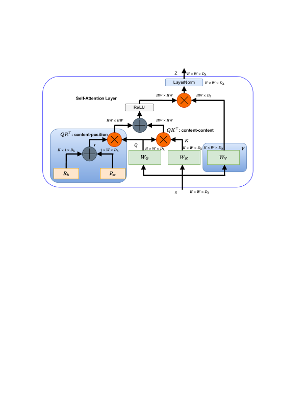
(5) MHSABlock performs a slightly modified version of MHSA, which is shown in Fig. 4. It uses a relative positional encoding instead of the absolute one as discussed in Sec. 3.1. Following [30], the relative positional encoding is applied to a query to obtain , where . and are the vectors of all ones. In this case, an attention is computed as follows:
| (27) |
Another modification is to use ReLU instead of softmax as an activation function. As described in Sec. 3.1, relationships between query and key (i.e., logits) are obtained by taking an inner-product of with , and then they are passed on to the softmax function such that the attention weights for the -th query sum to one. An immediate advantage of this modification is that ReLU is hardware-friendly as it only consumes one comparator and one multiplexer. According to [31], the accuracy of ReLU-based attention is comparable to that of the original softmax-based one. In addition, the attention weights become sparser, which assists the analysis of information flow in the model. Besides, LayerNorm [32] is added at the end of MHSABlock to stabilize gradients and facilitate the convergence.
By combining the above two modifications, the MHSA is computed as follows:
| (28) |
| (29) |
5 Implementation
In this section, we describe the FPGA implementation of the proposed model.
We first discuss the FPGA implementation of the proposed model described in Sec. 4. The proposed system takes a software-hardware co-design approach. The PL (Programmable Logic) part of the FPGA receives pre-processed feature maps from the PS (Processing System) part. Subsequently, the PL part processes these feature maps and returns the output to the PS part. Then, the PS part performs image classification by running the post-processing part. Specifically, the feature extraction, i.e., the forward propagation from ODEBlock1 to MHSABlock (Fig. 2, right), is carried out on the PL part. The pre- and post-processing parts are performed on the PS part with ARM Cortex-A53 CPU @1.2GHz. The operating frequency of the PL part is set to 150MHz.
As described in Sec. 4, our proposed model significantly reduces parameter size, and thus essential parameters for the feature extraction part can be stored in on-chip BRAM and URAM buffers. That is, only input and output data are transferred between the PL part and DRAM during inference. In this case, because the data transfer amount is quite small, the performance of the proposed design is compute-bound. In our FPGA implementation, the model assumes the input image resolution of 96 96. Note that the input image size has less impact on the model’s overall size because only the final fully-connected layer is adjusted depending on the image size and the feature extraction part is not affected.
Our FPGA implementation has two modes, which can be selected by control registers. One mode involves the transfer of weights and LUTs for quantization from DRAM to the PL part. This ensures that the necessary parameters are stored in on-chip buffers. The other mode is for inference based on the trained parameters.
5.1 Board-level implementation
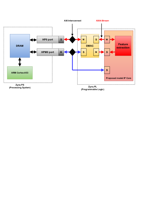
Fig. 5 depicts the block diagram of the proposed software-hardware co-design. The feature extraction part of the proposed model (i.e., from ODEBlock1 to MHSABlock) is implemented as a custom IP core. The custom IP core along with a DMA (Direct Memory Access) controller is implemented on the PL part. The DMA controller (DMAC) is in charge of transferring the input/output feature maps as well as the model parameters (e.g., LUTs for activations, quantized weights, and relative positional encoding) via AXI-Stream, and is connected to the 128-bit High-Performance (HP0) port. The IP core provides control registers for setting necessary configuration such as the number of ODE iterations. The PS part accesses these control registers through a 32-bit AXI-Lite interface (Fig. 5, blue lines). The pre- and post-processing blocks are also executed on the PS part.
5.2 FPGA implementation of the proposed model
The proposed model consists of three types of blocks: ODEBlock, MHSABlock, and DSBlock. In our implementation, all layers in each block are parallelized along the output channel dimension by utilizing multiple DSP blocks. We describe the implementation of ODEBlock and MHSABlock in the following.
5.2.1 Implementation of ODEBlock
The number of iterations for each ODEBlock is specified through respective control registers. ODEBlock keeps track of a time variable ( in Eq. (17)) during iterations (). The module “Add time” in Table 1 is to insert an additional channel filled with a time variable to the layer input; thus, this increases the number of output channels by one. In addition to on-chip buffers for weight parameters, extra buffers are allocated to retain the input to the block for skip connection and the output of each layer.
5.2.2 Implementation of MHSA
MHSA (Fig. 4) is executed in the following sequence: (1) Three weights , , and , along with pre-trained and for positional encoding, are transferred to the on-chip buffers. Then, (2) , , and are calculated sequentially for input . (3) For positional encoding, and are calculated sequentially. (4) is added to the positional encoding (i.e., ). Afterward, (5) is divided by a scaling factor . (6) ReLU is applied for to acquire an attention . Subsequently, (7) is calculated for input . (8) A dot product of and is calculated. Finally, (9) LayerNorm is applied for the output of MHSA.
5.3 Quantization of layers
Furthermore, the design performs an LUT-based quantization as described in Sec. 3.3. The accuracy with respect to different quantization levels is evaluated in Sec. 6.2.3. Except the first and last layers in the model, each fully-connected/convolution layer has two learnable LUTs for weights and activations. The LUTs for weights are not necessary during inference, and thus only -bit quantized weights are stored on-chip, which are computed by a host CPU at initialization. On the other hand, the LUTs for activations are transferred to the PL part, since the activations are quantized during inference. In addition, the scaling parameters and are transferred. The quantization of a single layer introduces additional parameters for one LUT and two scaling parameters, which increase the on-chip memory footprint by bits. On the other hand, the memory consumption for weights reduces from to bits, where denotes the number of weight parameters in a layer. We assume as in [26]. In this case, the following inequality should be satisfied for the quantization to be effective.
| (30) |
We can derive that when and when . In our model, the quantization is applied to depth-wise/point-wise convolution layers present in ODEBlock1-2 and MHSABlock. These convolution layers have 585 to 16,448 parameters and thus Eq. (30) holds in most cases except the smallest layer. The memory reduction rate is calculated as follows:
| (31) |
For instance, the point-wise convolution layer in MHSABlock, which is the largest in the model, achieves 3.51 and 6.99 reduction when and , respectively. In typical cases where , Eq. (31) can be approximated as .
The layer input is in full-precision and quantized according to Eqs. (25) and (26) to obtain . The layer computations such as convolutions are performed using the quantized and . While the weights are maintained as signed -bit integers, it should be noted that during calculations, the -bit weights are scaled by to obtain the full-precision weight .
| Block | Output size | Input/output channels | Architecture |
| Pre-processing | 3 (RGB) 64 | Conv | |
| 64 64 | Max pool, stride 2 | ||
| ODEBlock1 | 64 65 | Add time | |
| 65 64 | DSC | ||
| 64 64 | BatchNorm | ||
| 64 64 | ReLU | ||
| 64 65 | Add time | ||
| 65 64 | DSC | ||
| 64 64 | BatchNorm | ||
| DSBlock1 | 64 128 | Conv, stride 2 | |
| 128 128 | BatchNorm | ||
| 128 128 | ReLU | ||
| 128 128 | Conv, stride 1 | ||
| 128 128 | BatchNorm | ||
| 128 128 | ReLU | ||
| ODEBlock2 | 128 129 | Add time | |
| 129 128 | DSC | ||
| 128 128 | BatchNorm | ||
| 128 128 | ReLU | ||
| 128 129 | Add time | ||
| 129 128 | DSC | ||
| 128 128 | BatchNorm | ||
| DSBlock2 | 128 256 | Conv, stride 2 | |
| 256 256 | BatchNorm | ||
| 256 256 | ReLU | ||
| 256 256 | Conv, stride 1 | ||
| 256 256 | BatchNorm | ||
| 256 256 | ReLU | ||
| MHSABlock | 256 257 | Add time | |
| 257 64 | Conv | ||
| 64 64 | BatchNorm | ||
| 64 64 | MHSA | ||
| 64 65 | Add time | ||
| 65 256 | Conv | ||
| 256 256 | ReLU | ||
| Post-processing | * | Average pool | |
| * | Linear |
6 Evaluations
We compare the proposed model with ODENet [27], BoTNet [7], ViT [2], and lightweight CNN-based architectures such as ResNet18, EfficientNet [33], EfficientNetV2 [34], MobileNet V2 [35], and MobileNet V3 [36] in terms of parameter size and accuracy. Furthermore, we conduct ablation studies to explore the trade-off between accuracy and resource utilization. We investigate the effectiveness of the newly added MHSABlock and the impact of LUT-based quantization on accuracy.
6.1 Experimental setup
6.1.1 STL10 dataset
The proposed model is a combination of CNN and attention mechanism. Since the attention mechanism aims to aggregate global information, it is expected to be beneficial in case of larger input images. As discussed in Sec. 2.1, such a hybrid model can achieve a high accuracy even with small datasets compared to pure attention-based models (e.g., ViT). To demonstrate the benefit of the proposed hybrid model, we compare its performance with ViT-Base [2] with a relatively small STL10 [37] dataset containing 10 object classes. STL10 contains 50k labeled images of pixels for training and 8k for testing. While CIFAR-10/100 [12] datasets are widely used for image classification models, they contain smaller images (e.g., ) than STL10.
6.1.2 Model training
All network models considered here are implemented with Python 3.8.10 and PyTorch 1.12.1. The proposed model is built based on the code used in [27]. In our proposed model, DSC is applied to ODEBlocks while it is not applied to DSBlocks. In addition, by applying DSC to DSBlock1, DSBlock2, and both of them, we build three variant models, referred to as “DS1DSC”, “DS2DSC”, and “DS12DSC”, respectively. In this paper, we used the same hyperparameters for training except the batch size; specifically, the batch size is set to 5 for the proposed model, and 128 for the others. The number of epochs is set to 310, and SGD is used as an optimizer. We set the weight decay to and the momentum to 0.9. The cosine annealing with warm restart is used as a learning rate scheduler. The initial learning rate is set to 0.1, and the minimum learning rate is set to . For data augmentation, the training images were randomly flipped, erased with a probability of 0.5, and jittered.
| Model | Parameter size | MHSA |
|---|---|---|
| ResNet50 | 23.52M | |
| BoTNet50 [7] | 18.89M | ✓ |
| ODENet [27] | 1.29M | |
| Proposed model | 1.26M | ✓ |
| Proposed model (DS1DSC) | 1.08M | ✓ |
| Proposed model (DS2DSC) | 0.51M | ✓ |
| Proposed model (DS12DSC) | 0.33M | ✓ |
| ViT-Base [2] | 78.22M | ✓ |
| ResNet18 | 14.19M | |
| EfficientNetb0 [33] | 5.33M | |
| EfficientNetv2s [34] | 21.61M | |
| MobileNet V2 [35] | 3.54M | |
| MobileNet V3 [36] | 2.56M |
6.2 Evaluation results
6.2.1 Parameter size
Table 2 shows the parameter size of the proposed and counterpart models with and without MHSA mechanism. As shown, the proposed model uses the smallest number of parameters among these lightweight models, thanks to the benefits of Neural ODE. BoTNet50 has 1.24 less parameters than ResNet50, because convolutions in the last three ResBlocks are replaced by MHSA. Our proposed model achieves 14.96 reduction from BoTNet50 by combining MHSA and Neural ODE; as described in Sec. 3, the use of Neural ODE allows to compress ResBlocks into one ODEBlock, yielding -fold reduction. In our case, , i.e., the number of ODE solver iterations, is set to 10. By employing DSC instead of the original convolution in DSBlocks, the parameter size can be further reduced by up to 3.86 (see DS1DSC, DS2DSC, and DS12DSC in Table 2). Compared to our proposed model, ViT-Base is 61.96 larger, making it unsuitable for resource-limited devices due to its high computational cost. While EfficientNet and MobileNet are designed with the deployment on mobile devices in mind, they still have 2.02–17.12 more parameters than ours, and also do not benefit from the attention mechanism.
| Model | Top-1 accuracy (%) | MHSA |
|---|---|---|
| ResNet50 | 79.20 | |
| BoTNet | 81.60 (+2.40) | ✓ |
| ODENet | 79.11 | |
| Proposed model | 80.15 (+1.04) | ✓ |
| Proposed model (DS1DSC) | 80.05 | ✓ |
| Proposed model (DS2DSC) | 79.95 | ✓ |
| Proposed model (DS12DSC) | 79.29 | ✓ |
| ViT-Base | 62.59 | ✓ |
| ResNet18 | 72.43 | |
| EfficientNetb0 | 74.96 | |
| EfficientNetv2s | 75.05 | |
| MobileNet V2 | 72.56 | |
| MobileNet V3 | 77.26 |
6.2.2 Classification accuracy
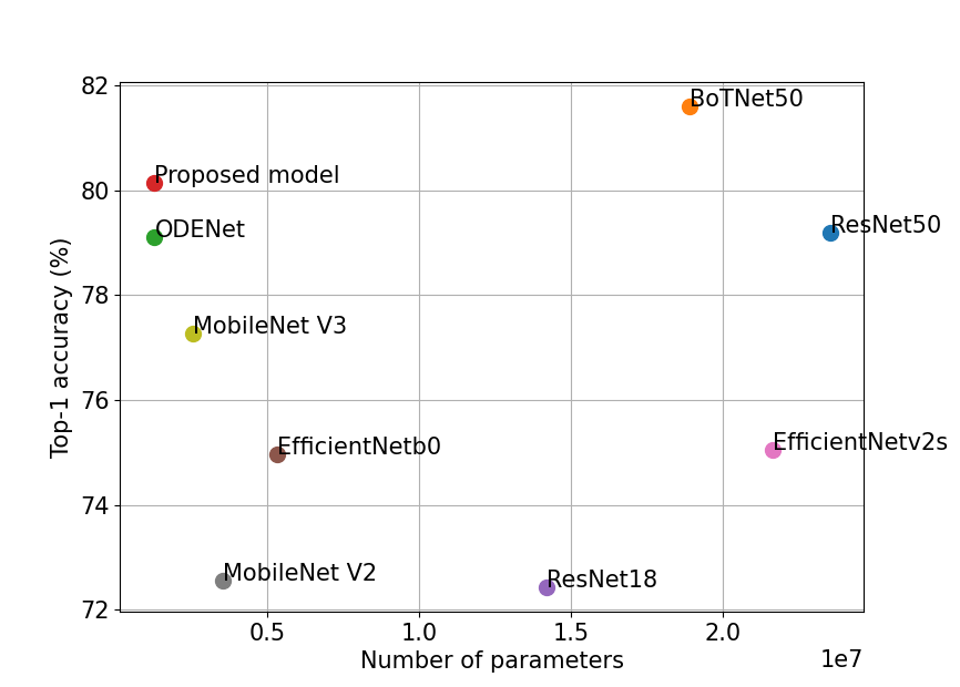
Table 3 presents the top-1 accuracy of each model with STL10 dataset. BoTNet shows 2.4% higher accuracy than ResNet50, owing to the attention blocks placed at the end. Analogous to this, our proposed model achieves 1.04% accuracy improvement over ODENet. The proposed model which simplifies the architecture of BoTNet by introducing the concept of Neural ODE leads to a similar improvement on accuracy. While our proposed model has 14.96 less parameters than BoTNet, it offers comparable accuracy and hence greatly improves the trade-off between accuracy and computational cost. In addition, it achieves 2.89–7.72% better accuracy than EfficientNet and MobileNet series. Fig. 6 visualizes the top-1 accuracy and parameter size of different models. The proposed model is in the top-left most corner, highlighting the better accuracy-computation trade-off. Due to the scaling laws between the number of parameters and accuracy in AI models, models positioned in the upper left of the diagram tend to offer a favorable trade-off.
6.2.3 Effects of quantization
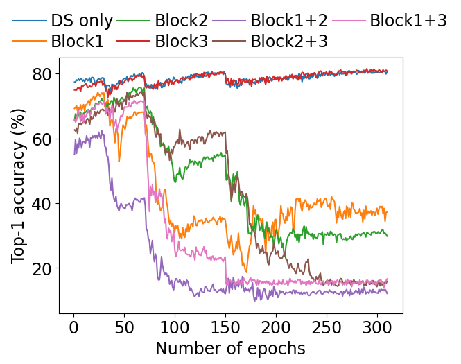
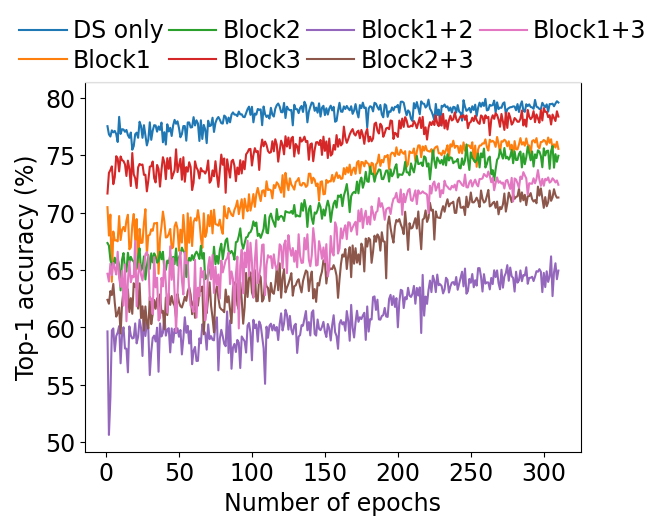
To reduce the memory footprint and implement the proposed model on modest-sized FPGAs, we want to apply quantization to as many layers as possible. On the other hand, since there is a trade-off between the degree of quantization and accuracy, there is a risk of significant accuracy degradation if quantization is applied to all layers without careful consideration. Here, we conduct ablation studies to investigate the impact of learning rates on the quantized blocks. We evaluate different combinations of quantized blocks. It should be noted that quantization is always applied to DSBlocks that are used only once in a single inference. We expect quantization on these blocks has less impact on accuracy. DSC is applied to ODEBlocks only. The initial and minimum learning rates for the cosine annealing scheduler are set to (5e-3, 1e-5), (5e-4, 1e-5), and (1e-4, 1e-5).
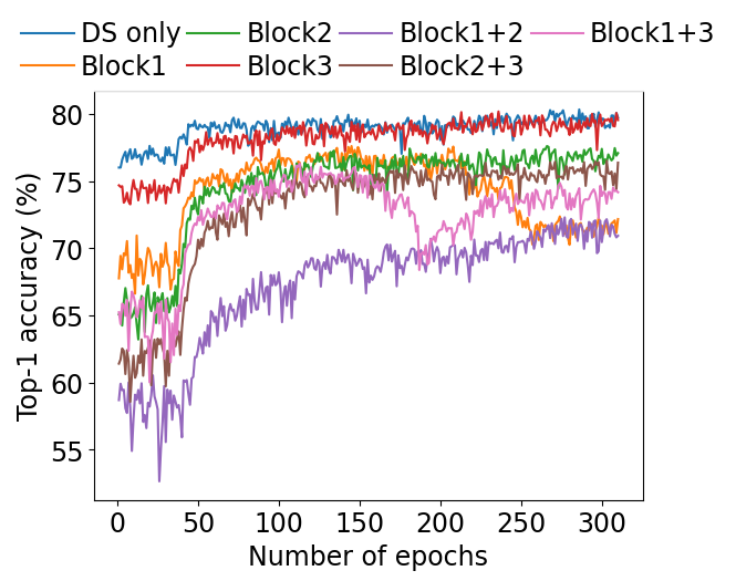
Fig. 7 shows the evaluation results. In these graphs, “DS only” indicates that the quantization is applied to DSBlocks only. “Block1”, “Block2”, and “Block3” refer to the proposed models with the quantized ODEBlock1, ODEBlock2, and MHSABlock, respectively. “Block1+2” refers to the model with both ODEBlock1 and ODEBlock2 quantized. When the learning rate is high as shown in Fig. 7(a), the training process fails to converge, leading to a significant accuracy loss especially after 150 epochs due to warm restart. In Fig. 7(b), on the other hand, the training succeeds in all the settings. In Fig. 7(c), while the accuracy improves with the number of epochs, the final accuracy of the models with quantized ODEBlock/MHSABlock is slightly lower compared to that in Fig. 7(b), suggesting that the learning rate used is not optimal. Considering that Block3 gives almost the same performance as the DS only setting and achieves higher accuracy than Block1 and Block2, MHSABlock is more tolerant to quantization than ODEBlocks. In addition, while ODEBlock2 contains more parameters than ODEBlock1, Block2 obtains better results than Block1. This implies that the having more parameters in a block does not necessarily increase its sensitivity to quantization.
6.2.4 FPGA resource utilization
Table 4 presents the FPGA resource utilization of the proposed model with 4-bit and 8-bit quantization applied to all building blocks. Thanks to the quantization and the 14.96 parameter size reduction by Neural ODE, the feature extraction part of our model fits within the on-chip BRAM/URAM. The quantized weight parameters are mostly stored in URAM. As a result, compared to the 8-bit quantization, the URAM utilization is further reduced by 17.7% with the aggressive 4-bit quantization.
| Model | BRAM | DSP | FF | LUT | URAM |
|---|---|---|---|---|---|
| Available | 624 | 1,728 | 460,800 | 230,400 | 96 |
| 4-bit quantization | 589 | 206 | 24,143 | 66,843 | 29 |
| 94.4 | 11.92 | 5.24 | 29.01 | 30.21 | |
| 8-bit quantization | 595 | 206 | 23,681 | 66,292 | 46 |
| 95.4 | 11.92 | 5.14 | 28.77 | 47.92 |
| Model | Mean | Max | Std |
| CPU (8-bit quantization) | 1,596 | 1,676 | 12.73 |
| CPU (4-bit quantization) | 1,590 | 1,640 | 9.27 |
| FPGA (8-bit quantization) | 130 | 130 | 0.03 |
| FPGA (4-bit quantization) | 125 | 125 | 0.03 |
6.2.5 Execution time
In this section, we compare the performance of our FPGA implementation with its software counterpart running on ARM Cortex-A53 CPU. The software counterpart is implemented with PyTorch. The 8-bit and 4-bit quantizations are applied to both the implementations, respectively. Table 5 presents the mean, maximum, and standard deviation of the execution time obtained by 100 runs. In the 8-bit case, the average inference time is reduced from 1,596ms to 130ms per input feature map, yielding a 12.3 speedup. Similarly, our FPGA implementation with the 4-bit quantization runs in 125ms, which is 12.8 faster than the software implementation.
6.2.6 Energy efficiency
The power consumption of the proposed FPGA implementation is evaluated based on power reports from Xilinx Vivado. For both the 8-bit and 4-bit quantized models, the power consumption in the PS part is 2.64W, while that of the proposed IP core is 1.02W. Considering that the inference times of the 8-bit and 4-bit quantized models are accelerated by 12.3 and 12.8, the energy efficiency is improved by 8.85 and 9.21, respectively.
7 Summary
Transformers, featuring the highly expressive MHSA mechanism, have demonstrated remarkable accuracy in the field of image processing among recent AI models. This paper focuses on a hybrid model that combines Transformer and CNN architectures. Considering the resource constraints of edge devices, we employed Neural ODE, an approximation technique inspired by ResNet, to design a tiny CNN-Transformer hybrid model with 94.6% less parameters than ResNet50. The parameter size of the proposed model is the smallest among the state-of-the-art lightweight models while it offers a comparable accuracy. We proposed the resource-efficient FPGA design of the tiny Transformer model tailored for edge devices. We employed a recently-proposed LUT-based quantization technique and conducted the ablation studies to investigate the impact of quantization on different parts of the proposed model. We implemented the entire feature extraction part on a modest-sized FPGA to accelerate inference speed. Compared to an embedded CPU, our FPGA implementation achieved 12.8 faster runtime and 9.21 higher energy efficiency. Thanks to the small parameter size and quantization, the parameters fit within the limited on-chip memory, eliminating unnecessary data transfer overhead. Using high-end FPGAs would allow more design choices and further optimizations, potentially leading to greater improvements on the speed and accuracy.
References
- [1] A. Vaswani et al., “Attention is All you Need,” in Proceedings of the Advances in Neural Information Processing Systems (NeurIPS), Jun 2017, pp. 5998–6008.
- [2] A. Dosovitskiy et al., “An Image is Worth 16x16 Words: Transformers for Image Recognition at Scale,” in Proceedings of the International Conference on Learning Representations (ICLR), Jan 2021, pp. 1–21.
- [3] C. Sun et al., “Revisiting Unreasonable Effectiveness of Data in Deep Learning Era,” in Proceedings of the IEEE/CVF International Conference on Computer Vision (ICCV), Oct 2017, pp. 843–852.
- [4] K. Yuan et al., “Incorporating Convolution Designs into Visual Transformers,” in Proceedings of the IEEE/CVF International Conference on Computer Vision (ICCV), Oct 2021, pp. 579–588.
- [5] H. Wu et al., “CvT: Introducing Convolutions to Vision Transformers,” in Proceedings of the IEEE/CVF International Conference on Computer Vision (ICCV), Oct 2021, pp. 22–31.
- [6] A. Trockman et al., “Patches Are All You Need?” arXiv:2201.09792, Jan 2022.
- [7] A. Srinivas et al., “Bottleneck Transformers for Visual Recognition,” in Proceedings of the IEEE Conference on Computer Vision and Pattern Recognition (CVPR), Aug 2021, pp. 16 514–16 524.
- [8] N. Park et al., “How Do Vision Transformers Work?” in Proceeding of the International Conference on Learning Representations (ICLR), Apr 2022, pp. 1–26.
- [9] Z. Dai et al., “CoAtNet: Marrying Convolution and Attention for All Data Sizes,” arXiv:2106.04803, Jun 2021.
- [10] I. Okubo et al., “A Lightweight Transformer Model using Neural ODE for FPGAs,” in Proceedings of the IEEE International Parallel and Distributed Processing Symposium Workshops (IPDPSW), May 2023, pp. 105–112.
- [11] R. T. Q. Chen et al., “Neural Ordinary Differential Equations,” in Proceedings of the Advances in Neural Information Processing Systems (NeurIPS), Dec 2018, pp. 6571–6583.
- [12] A. Krizhevsky, “Learning Multiple Layers of Features from Tiny Images,” University of Toronto, Tech. Rep., Apr 2009.
- [13] O. Russakovsky et al., “ImageNet Large Scale Visual Recognition Challenge,” International Journal of Computer Vision (IJCV), vol. 115(3), pp. 211–252, Dec 2015.
- [14] N. Kitaev et al., “Reformer: The Efficient Transformer,” in Proceedings of the International Conference on Learning Representations (ICLR), Apr 2020, pp. 1–12.
- [15] A. Katharopoulos et al., “Transformers are RNNs: Fast Autoregressive Transformers with Linear Attention,” in Proceedings of the International Conference on Machine Learning (ICML), Jul 2020, pp. 5156–5165.
- [16] S. Wang et al., “Linformer: Self-Attention with Linear Complexity,” arXiv:2006.04768, Jun 2020.
- [17] T. Dao et al., “FlashAttention: Fast and Memory-Efficient Exact Attention with IO-Awareness,” in Proceedings of the Advances in Neural Information Processing Systems (NeurIPS), Nov 2022, pp. 16 344–16 359.
- [18] Z. Liu et al., “Swin Transformer: Hierarchical Vision Transformer using Shifted Windows,” in Proceedings of the IEEE/CVF International Conference on Computer Vision (ICCV), Mar 2021, pp. 10 012–10 022.
- [19] X. Liu et al., “Neural SDE: Stabilizing Neural ODE Networks with Stochastic Noise,” arXiv:1906.02355, Jun 2019.
- [20] C. Finlay et al., “How to Train Your Neural ODE: the World of Jacobian and Kinetic Regularization,” in Proceedings of the International Conference on Machine Learning (ICML), Jul 2020, pp. 3154–3164.
- [21] H. Yan et al., “On Robustness of Neural Ordinary Differential Equations,” arXiv:1910.05513, Oct 2019.
- [22] E. Dupont et al., “Augmented Neural ODEs,” in Proceedings of the Advances in Neural Information Processing Systems (NeurIPS), Dec 2019, pp. 3140–3150.
- [23] H. Peng et al., “Accelerating Transformer-based Deep Learning Models on FPGAs using Column Balanced Block Pruning,” Apr 2021, pp. 142–148.
- [24] B. Li et al., “FTRANS: Energy-Efficient Acceleration of Transformers Using FPGA,” in Proceedings of the ACM/IEEE International Symposium on Low Power Electronics and Design (ISLPED), Aug 2020, pp. 175–180.
- [25] M. Sun et al., “VAQF: Fully Automatic Software-Hardware Co-Design Framework for Low-Bit Vision Transformer,” arXiv:2201.06618, Jan 2022.
- [26] L. Wang et al., “Learnable Lookup Table for Neural Network Quantization,” in Proceedings of the IEEE Conference on Computer Vision and Pattern Recognition (CVPR), Sep 2022, pp. 12 423–12 433.
- [27] H. Kawakami et al., “dsODENet: Neural ODE and Depthwise Separable Convolution for Domain Adaptation on FPGAs,” in Proceeding of the Euromicro International Conference on Parallel, Distributed, and Network-Based Processing (PDP), Mar 2022, pp. 152–156.
- [28] A. G. Howard et al., “MobileNets: Efficient Convolutional Neural Networks for Mobile Vision Applications,” arXiv:1704.04861, Apr 2017.
- [29] F. Chollet, “Xception: Deep Learning with Depthwise Separable Convolutions,” in Proceedings of the IEEE Conference on Computer Vision and Pattern Recognition (CVPR), Jul 2017, pp. 1800–1807.
- [30] I. Bello et al., “Attention Augmented Convolutional Networks,” in Proceedings of the IEEE/CVF International Conference on Computer Vision (ICCV), Nov 2019, pp. 3286–3295.
- [31] B. Zhang et al., “Sparse Attention with Linear Units,” in Proceedings of the Conference on Empirical Methods in Natural Language Processing (EMNLP), Nov 2021, pp. 6507–6520.
- [32] ——, “Root Mean Square Layer Normalization,” in Proceedings of the Neural Information Processing Systems (NeuralIPS), Oct 2019, pp. 12 360–12 371.
- [33] M. Tan and Q. Le, “EfficientNet: Rethinking Model Scaling for Convolutional Neural Networks,” in Proceedings of the International Conference on Machine Learning (PMLR), Jun 2019, pp. 6105–6114.
- [34] ——, “EfficientNetV2: Smaller Models and Faster Training,” in Proceedings of the International Conference on Machine Learning (PMLR), Jul 2021, pp. 10 096–10 106.
- [35] M. Sandler et al., “MobileNetV2: Inverted Residuals and Linear Bottlenecks,” in Proceedings of the IEEE Conference on Computer Vision and Pattern Recognition (CVPR), Jun 2018, pp. 4510–4520.
- [36] S. Qian et al., “MobileNetV3 for Image Classification,” in Proceeding of the IEEE International Conference on Big Data, Artificial Intelligence and Internet of Things Engineering (ICBAIE), Mar 2021, pp. 490–497.
- [37] A. Coates et al., “An Analysis of Single-Layer Networks in Unsupervised Feature Learning,” in Proceedings of the International Conference on Artificial Intelligence and Statistics (AISTATS), Apr 2011, pp. 215–223.