Long-Range Four-body Interactions in Structured Nonlinear Photonic Waveguides

Abstract

Multi-photon dynamics beyond linear optical materials are of significant fundamental and technological importance in quantum information processing. However, it remains largely unexplored in nonlinear waveguide QED. In this work, we theoretically propose a structured nonlinear waveguide in the presence of staggered photon-photon interactions, which supports two branches of gaped bands for doublons (i.e., spatially bound-photon-pair states). In contrast to linear waveguide QED systems, we identify two important contributions to its dynamical evolution, i.e., single-photon bound states (SPBSs) and doublon bound states (DBSs). Most remarkably, the nonlinear waveguide can mediate the long-range four-body interactions between two emitter pairs, even in the presence of disturbance from SPBS. By appropriately designing system’s parameters, we can achieve high-fidelity four-body Rabi oscillations mediated only by virtual doublons in DBSs. Our findings pave the way for applying structured nonlinear waveguide QED in multi-body quantum information processing and quantum simulations among remote sites.

Introduction.—The past few years have witnessed a surge of interest in the field of waveguide quantum electrodynamics (QED) in structured linear optical materials without photon-photon interactions, leading to intriguing phenomena such as unconventional bound states, non-Markovian evolution and chiral emissions Mitsch et al. (2014); Lodahl et al. (2015); Douglas et al. (2015); Bliokh and Nori (2015); Shi et al. (2016); Lodahl et al. (2017); González-Tudela and Cirac (2017); Liu and Houck (2017); Trainiti and Ruzzene (2016); Chang et al. (2018); García-Elcano et al. (2020); Tang et al. (2022); Wang and Li (2022); Stewart et al. (2020); De Bernardis et al. (2023). In these linear optical waveguides, dynamical properties are governed and investigated at the single-photon level Karplus and Neuman (1951); Iacopini and Zavattini (1979); Scully and Zubairy (1997); Cohen-Tannoudji et al. (1998); Walls and Milburn (2007); Zhou et al. (2008); Liao et al. (2010); Agarwal (2012). However, once quantum many-body interactions between individual photons are introduced, standard descriptions based on single-photon properties are inadequate Imamoḡlu et al. (1997); Liao and Law (2010); Peyronel et al. (2012); Dudin et al. (2012); Chang et al. (2014); Dorfman et al. (2016); Roy et al. (2017); Kruk et al. (2018); Mahmoodian et al. (2018a); Ke et al. (2019); Poshakinskiy and Poddubny (2021); Marques et al. (2021); Sheremet et al. (2023). These nonlinear quantum optics phenomena can find important applications in fields of quantum information and metrology Napolitano et al. (2011); Reiserer et al. (2013); Shomroni et al. (2014); Mahmoodian et al. (2018b); Cordier et al. (2023).

In artificial platforms, such as nanophotonic structures and circuit-QED, strong nonlinear interactions can be experimentally realized Cramer et al. (2008); Ma et al. (2019); Eckardt (2017); Rubio-Abadal et al. (2020); Kuo et al. (2020); Zhu et al. (2022), providing ideal platforms for exploring quantum effects at the level of few photons, and effects of many-body statistics on waveguide QED Gemelke et al. (2009); Macha et al. (2014); Weißl et al. (2015); Kaufman et al. (2016); Salathé et al. (2015); Reithmaier et al. (2015); Roushan et al. (2017); Yan et al. (2019); Chang et al. (2020); Carusotto et al. (2020); Kim et al. (2021); Scigliuzzo et al. (2022); Qiao and Gong (2022); Zhang et al. (2023). Recently, a remarkable supercorrelated radiance phenomenon, beyond the conventional super- and subradiance, was reported in a nonlinear waveguide QED system with non-structured bath Wang et al. (2020). Until now, in spite of potentially interesting physics hidden behind it, the field of nonlinear waveguide QED remains largely unexplored. Along previous works in this field Wang et al. (2020); Talukdar and Blume (2022a, b, 2023), a natural question arises: how the structured nonlinear waveguide QED system influences the dynamics in the presence of a strong photon-photon interaction.

Here we consider emitter pairs interacting with a structured nonlinear waveguide by designing a staggered onsite photon-photon interaction. In contrast to previous work Wang et al. (2020); Talukdar and Blume (2022a, b, 2023), we find the formation of gaped bands for doublons, i.e., spatially bound-photon-pair states Winkler et al. (2006); Piil and Mølmer (2007); Wang and Liang (2010); Di Liberto et al. (2016); Gorlach and Poddubny (2017); Calajó et al. (2016); Tai et al. (2017); Lyubarov and Poddubny (2019); Chen et al. (2020); Flannigan and Daley (2020); Stepanenko and Gorlach (2020); Xing et al. (2021); Berti and Carusotto (2022); Stepanenko et al. (2022). We reveal the effects of both doublon bound states (DBSs) and single-photon bound states (SPBSs) on the evolution dynamics of the hybrid system. Most remarkably, we demonstrate long-range four-body interactions, mediated by DBSs, between distant emitter pairs. We find that a large high-fidelity four-body interaction requires two emitter pairs for a separation larger than the size of the SPBS, to prevent undesired single-photon-mediated transitions. Our study shows a remarkable different physics in the nonlinear waveguide QED regime in contrast with conventional linear systems.

Figure 1: Schematic of the nonlinear QED setup, with a waveguide consisting of coupled cavity arrays in the presence of a Kerr nonlinearity. Here, $J$ is the photonic hopping strength, and $U_{\pm}=U_{c}\pm U_{m}$ denotes the staggered onsite photon-photon interaction. The emitter pair $e_{1,2}$ is separated from the pair $e_{3,4}$ by a distance $D_{q}$, while $d_{1}^{e}$ and $d_{2}^{e}$ are the distance of each emitter pair. In the dynamical evolution, a doublon bound state (DBS), corresponding to a virtual exchange process of two photons with correlated length $L_{c}$, is considered, accompanied by single-photon bound state (SPBSs) due to the virtual exchange of a single photon.

Doublon band.—We consider a nonlinear waveguide constructed by an array of coupled cavities in the presence of strong photon-photon interactions (see Fig. 1). In the rotating frame of the cavity frequency, the Hamiltonian of the waveguide is written as

$$H_{w}=-J\sum_{n}(a^{\dagger}_{n}a_{n+1}+\text{H.c.})-\frac{1}{2}\sum_{n}U_{n}a^{\dagger}_{n}a^{\dagger}_{n}a_{n}a_{n},$$ (1)

where $J$ is the bosonic hopping strength, and $U_{n}$ denotes the Kerr nonlinearity at site $n$. To realize a structured environment, we introduce the staggered photon-photon interaction with $U_{n}=U_{c}+(-1)^{n}U_{m}$ (where $U_{c}\pm U_{m}$ is the staggered interaction strength). We calculate the two-photon spectrum as a function of $U_{c}$ for a finite waveguide of length $N$ (by setting $J=1$), as shown in Fig. 2(a). Besides continuum scattering states, there exist discrete doublon energy bands with bound photon pairs. In addition, the doublon bands become distinctly separated from the scattering states for $U_{c}>4J$.

The two-photon spectrum can be analytically solved by defining the center-of-mass and relative coordinates, i.e., $x_{c}=(m+n)/2$ and $r=m-n$, with $m$ and $n$ representing the positions of the two photons. As explained in the Supplemental Material sup , the eigenenergy $E$ and the center-of-mass $K$ of a doublon state satisfy the following relationship

$$\det\left|\begin{matrix}\frac{U_{c}}{U_{\cos}}-1&\frac{U_{m}}{U_{\cos}}\vspace{1ex}\\ \frac{U_{m}}{U_{\sin}}&\frac{U_{c}}{U_{\sin}}-1\\ \end{matrix}\right|=0.$$ (2)

where $U_{\cos}=\{E^{2}-16\left[J\cos\left(K/2\right)\right]^{2}\}^{1/2}$, and $U_{\sin}=\{E^{2}-16\left[J\sin\left(K/2\right)\right]^{2}\}^{1/2}$. We plot two branches of the doublon bands in Fig. 2(b) according to Eq. (2), where a band gap exists. In particular, at the band edge with zero group velocity, the wavefuntions $\Psi^{\pm}_{K}$ at $K_{0}=\pi/2$ of two bands can be analytically obtained as sup

$$\Psi^{\mp}_{K_{0}}\left(x_{c},r\right)=\frac{e^{iK_{0}x_{c}}}{\sqrt{N}\psi_{0}}\left(1\pm e^{i\pi x_{c}}\right)\exp\left[-\frac{r}{L_{\mp}(K_{0})}\right],$$ (3)

where $\psi_{0}$ is the normalization factor, and $L_{\mp}(K_{0})$ are the decay lengths of the two-photon correlation function for mode $K_{0}$.

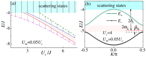
Figure 2: (a) Two-excitation spectrum of the Hamiltonian $H_{w}$ versus the mean value $U_{c}$. The cyan region on top corresponds to the scattering states, and the curves represent the upper and lower bounds of the doublon energy bands in Eq. (2). (b) Doublon’s spectrum for $U_{c}=4J$ and $U_{m}=0.05U_{c}$. The emitter-pair frequency $2\omega_{q}$ lies inside the doublon band gap with a detuning $\delta_{\mathrm{II}}$ ($2\delta_{\mathrm{I}}$) to the lower band (scattering states).

A strong on-site nonlinear interaction results in supercorrelated doublon modes sup . According to Eq. (3), $L_{\mp}(K_{0})\sim 1$ for $U_{c}\simeq 4J$, indicating that the two photons are strongly bunched in space.

Dynamics and bound states.—We first consider two emitters $e_{1}$ and $e_{2}$, which are separated by a distance $d^{e}_{1}$, interacting with the nonlinear waveguide at points $n_{1}$ and $n_{2}$ (see Fig. 1). The hybrid system’s Hamiltonian is

$$H=H_{w}+\frac{\omega_{q}}{2}\sum_{i=1}^{2}{\sigma_{i}^{z}}+g\sum_{i=1}^{2}{\left(\sigma_{i}^{+}a_{n_{i}}+\mathrm{H}.\mathrm{c}.\right)},$$ (4)

where $\omega_{q}$ is the emitter frequency, and $g$ is the coupling strength between each emitter and the waveguide. When the two-emitter excitation frequency $2\omega_{q}$ is set in the band gap between the doublon bands [see Fig. 2(b)], the evolution becomes highly non-Markovian owing to the van Hove singularity in the spectrum, which is different from the case of unstructured nonlinear waveguides Wang et al. (2020).

We now proceed to calculate the dynamics in the double-excitation subspace. We assume two emitters initially in their excited states, and their frequencies are chosen to be close to the lower band edge, with frequency detuning $\delta_{\mathrm{II}}=2\omega_{q}-E_{-}({K_{0}})\simeq 0$ [see Fig. 2(b)]. Since $H$ in Eq. (4) conserves the excitation number, in the double-excitation subspace, the state $|\psi_{2}\left(t\right)\rangle$ is

$$|\psi_{2}\left(t\right)\rangle = c_{e}\left(t\right)|ee,\mathrm{vac}\rangle+\sum_{K}{c_{K}\left(t\right)}|gg,\Psi^{-}_{K}\rangle$$ (5)

$$+\sum_{k}{\left[c_{1k}\left(t\right)|eg\rangle+c_{2k}\left(t\right)|ge\rangle\right]}a_{k}^{\dagger}|\mathrm{vac}\rangle,$$

where $c_{e}\left(t\right)$ [$c_{K}\left(t\right)$] is the probability amplitude for two emitters (doublon states $|\Psi^{-}_{K}\rangle$) being excited, $a_{k}^{\dagger}=\sum_{n}{e^{ikn}a_{n}^{\dagger}}/\sqrt{N}$ is the single-photon creation operator in momentum space, and $c_{ik}$ is the probability amplitude for the emitter $i$ and the mode $k$ being simultaneously excited. Because $\omega_{q}$ is significantly detuned from the scattering states (i.e., $\delta_{\mathrm{I}}=|\omega_{q}-2J|\gg g$), we have neglected their contributions in Eq. (5).

Figure 3: (a) Time-dependent probability of the two-emitter excitations $|c_{e}(t)|^{2}$, and single- and two-photon excitations $P_{1,2}(t)$ for initially two-emitter excitation. The coupling points are set at $n_{1,2}=0$. (b) Wavefunction profile of the SPBS and DBS (by restricting $r=0$) obtained via numerical simulations up to $t=10^{3}$. (c) 2D field distribution for the DBS. (d) Two-point correlation function $G_{2}(r)$ for the field in (c). Here we set $J=1$, $g=0.1$, $U_{c}=4$, $U_{m}=0.05U_{c}$, $\alpha\simeq 2$, and $\delta_{\mathrm{II}}=0.03$.

The single-emitter excitation contributes to the formation of SPBS by virtually exciting a single photon in the waveguide. The wavefunction of the SPBS from the emitter $i$ is approximately derived as sup

$$\psi_{i}(n)\simeq A_{s}\exp\left(-\frac{|n-n_{i}|}{L_{\mathrm{I}}^{\text{B}}}\right),$$

$$\frac{1}{L_{\mathrm{I}}^{\text{B}}}=\ln\frac{2J}{|\omega_{q}|-\sqrt{\omega_{q}^{2}-4J^{2}}},\quad A_{s}=\frac{gJ}{\sqrt{\omega_{q}^{2}-4J^{2}}},$$ (6)

where $L_{\mathrm{I}}^{\text{B}}$ ($A_{s}$) is the decay length (amplitude) of the SPBS. The emitter $i$ excites a SPBS, spreading in the waveguide around the site $n_{i}$. Meanwhile, the emitter $j$ excites another photon at $n_{j}$. The overlap between this two photon pairs and the doublon state $\Psi^{-}_{K}$ will excite the doublon mode $K$. The mechanism of this higher-order process can be verified from the effective transition rate between $c_{e}$ and $c_{K}$ sup , which is proportional to

$$F_{K}\left(n_{1},n_{2}\right)\!\propto\!\sum_{i,j=1,2}^{i\neq j}{\sum_{n}{\!\Psi^{-}_{K}\!\left(\frac{n+n_{j}}{2},n_{j}-n\right)\!\psi_{i}\left(n\right)}},$$ (7)

which is a correlation function with a decay length bounded by $\max\{L_{-}(K),L_{\mathrm{I}}^{\text{B}}\}$ Wang et al. (2020); sup . If $|n_{i}-n_{j}|\gg\max\{L_{-}(K),L_{\mathrm{I}}^{\text{B}}\}$, $F_{K}\left(n_{1},n_{2}\right)$ will decrease to zero.

In Fig. 3(a), we plot the dynamic evolution in a finite-size waveguide with $N=1000$. Since the two-emitter excitation frequency $2\omega_{q}$ lies inside the doublon band gap, the emitter pair is prevented from radiating doublons. Thus, part of their excitation is trapped in the form of DBS. By approximating the dispersion relation around $E_{-}(K_{0})$ as a quadratic form with curvature $\alpha$, i.e., $\Delta_{K}\simeq\delta_{\mathrm{II}}+\alpha\left(K-K_{0}\right)^{2}$ (see Sec. III of Ref. sup ), the analytical wavefunction of the DBS is derived as

$$\Psi_{d}(x_{c},r)\simeq A_{d}\left(1+e^{i\pi x_{c}}\right)\exp\left(-\frac{r}{L_{c}}-\frac{|x_{c}-x_{m}|}{L_{\mathrm{II}}^{\text{B}}}\right),$$

$$A_{d}=\frac{g^{2}F_{K_{0}}^{*}\left(n_{1},n_{2}\right)}{J\psi_{0}\sqrt{\delta_{\mathrm{II}}\alpha}},\quad L_{\mathrm{II}}^{\text{B}}=\sqrt{\frac{\alpha}{\delta_{\mathrm{II}}}},$$ (8)

where $x_{m}=n_{1}+n_{2}$.

In Fig. 3(b,c) we plot the long-time field distribution for single- and two-photon states, corresponding to SPBS and DBS described in Eq. (6,8). Figure 3(d) shows the corresponding two-point spatial correlation $G_{2}(r)$ at $t=10^{3}$. Because only the modes around $K_{0}$ are excited with high probabilities, the correlation length is approximated as $L_{c}\simeq L_{-}(K_{0})$, and two virtual photons in DBS are strongly bound [see Fig. 3(c)]. The decay length $L_{\mathrm{II}}^{\text{B}}$ can be adjusted by tuning $\delta_{\mathrm{II}}$ or band’s curvature $\alpha$. While both the amplitude and decay length of SPBS, $A_{s}$ and $L_{\mathrm{I}}^{\text{B}}$, decrease quickly as $\delta_{\mathrm{I}}$ increases. Therefore, by appropriately setting $2\omega_{q}$, both the amplitude and decay length of the DBS can be considerably larger than for the SPBSs, as shown in Fig. 3(b). This is also manifested in Fig. 3(a), where the single-photon probability $P_{1}=\sum_{i,k}|c_{ik}(t)|^{2}$, which is obtained numerically, is much lower than the two-photon probability $P_{2}=\sum_{K}|c_{K}(t)|^{2}$) after a long-time evolution.

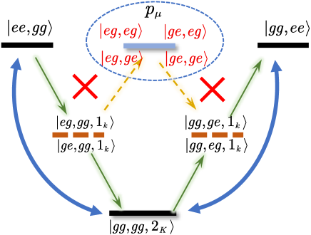
Figure 4: Illustration of the transitions mediated by the SPBSs and DBSs respectively. To enhance the fidelity of four-body Rabi oscillations, the unwanted single-photon transitions (represented by red crosses with amplitude $p_{\mu}$) should be suppressed.

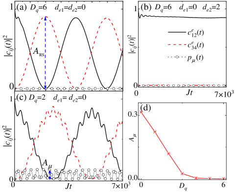
Figure 5: (a-c) Four-body Rabi oscillations between two emitter pairs under different distance conditions. The amplitude of the four-body Rabi oscillation (single-photon transitions) is denoted as $A_{\text{RS}}$ ($A_{\mu}$). (d) The single-photon transition amplitude $A_{\mu}$ versus $D_{q}$. Same parameters as in Fig. 3.

Four-body interactions.—The nonlinear waveguide can mediate four-body interactions. To demonstrate this, we consider two pairs of emitters coupled to the common nonlinear waveguide, as depicted in Fig. 1. The separation distance between the center of each pair is set as $D_{q}$. In the nonlinear waveguide, there are two kinds of virtual processes due to the wavefunction overlaps of DBSs for two emitter pairs, and SPBSs for emitters in different pairs. For the former case, the virtual exchange between two-doublon states leads to a four-body interaction associated with the transition $|ee,gg\rangle\leftrightarrow|gg,ee\rangle$, as shown in Fig. 4.

For the latter case, the virtual exchange of a single photon induced a conventional two-body interaction. For instance, as shown in Fig. 4, the overlap between two SPBSs of emitters 1 and 3 cause a two-body interaction associated with the transition $|ee,gg\rangle$ and $|ge,eg\rangle$. There exist four distinct single-photon transition paths (see Fig. 4), and the total oscillating amplitude is $P_{\mu}=\sum_{ij\neq 12,34}|c_{ij}^{e}(t)|^{2}$, where $c_{ij}^{e}(t)$ denotes the probability for emitter2, labelled by $i,j$, in the excited state.

The SPBS process complicates the dynamics of two-body interaction and reduces also the fidelity of four-body Rabi oscillations (see discussion below). In order to suppress the single-photon transition, the distance $D_{q}$ can be set as $\gg\!\!L_{\mathrm{I}}^{\text{B}}$, which prevents any overlap between the SPBSs of emitters in different pairs. We can achieve $P_{\mu}\simeq 0$ for the parameters considered in this work, and the effective four-body Hamiltonian is $H=J_{\text{RS}}\sigma_{1}^{-}\sigma_{2}^{-}\sigma_{3}^{+}\sigma_{4}^{+}+\text{H.c.}$ The four-body interaction strength $J_{\text{RS}}$ is

$$J_{\text{RS}}\simeq\frac{g^{4}F_{K_{0}}(n_{1},n_{2})F^{*}_{K_{0}}(n_{3},n_{4})}{J^{2}\sqrt{\delta_{\mathrm{II}}\alpha}}\exp\left(-\frac{D_{q}}{L_{\mathrm{II}}^{\text{B}}}\right),$$ (9)

which exponentially decreases as $D_{q}$, the same decay length as the DBS sup . In addition, emitters within the same pair are required to emit or absorb virtual photons concurrently. Therefore, $d^{e}_{1,2}$ should be considerably smaller than the correlation length of $F_{K}(n_{i},n_{j})$.

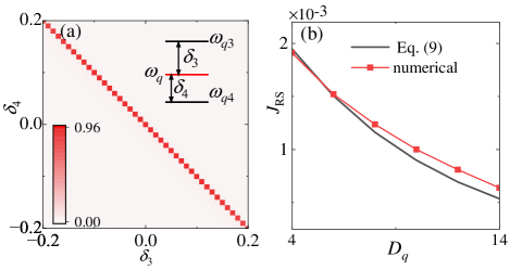
Figure 6: (a) Amplitude of the four-body Rabi oscillation $A_{\text{RS}}$ versus $\delta_{3,4}$. (b) The four-body interaction strength $J_{\text{RS}}$ versus $D_{q}$. The curve marked with symbols is obtained through numerical simulation, while the solid curve is plotted according to Eq. (9). Same parameters as in Fig. 4(a).

By adopting the appropriate parameters, we can realize with high-fidelity four-body Rabi oscillations (i.e., quasi-particle exchange in long-distance separation), associated to the four-body Hamiltonian. The four-body Rabi oscillations require

$$\begin{cases}1.\qquad d^{e}_{1,2}\ \leq\ \max\{L_{-}(K_{0}),\ L_{\mathrm{I}}^{\text{B}}\},\\ 2.\qquad L_{\mathrm{I}}^{\text{B}}\ \ll\ D_{q}\ \sim\ L_{\mathrm{II}}^{\text{B}}.\end{cases}$$ (10)

By considering the parameters in Fig. 3, the length scales can be computed as follows: $L_{\mathrm{II}}^{\text{B}}\simeq 9$, $L_{\mathrm{I}}^{\text{B}}\simeq 1.6$, and $L_{-}(K_{0})\simeq 1.4$, which can lead to the high-fidelity four-body Rabi oscillation. When $D_{q}$ and $d_{1,2}^{e}$ satisfy the conditions in Eq. (10), the four-body Rabi oscillation happens with a high fidelity, which amplitude is $A_{\text{RS}}\simeq 1$, as shown in Fig. 5(a). Once $d_{2}^{e}>2$, the second emitter pair cannot simultaneously absorb two virtual photons in the DBS. Consequently, the exchange process vanishes. Specifically, it is crucial to maintain a certain separation between the two pairs of emitters. When $D_{q}\approx L_{\mathrm{I}}^{\text{B}}$, the undesired transitions mediated by the SPBSs will disrupt the four-body Rabi oscillations, and the single-photon transition amplitude $A_{\mu}$ becomes larger, which can be confirmed by the evolution in Fig. 5(c). Numerical results in Fig. 5(d) indicate that transitions mediated by the SPBSs are negligible ($A_{\mu}\simeq 0$) when $D_{q}>4$.

In Fig. 6(a), we plot $A_{\text{RS}}$ versus the frequency detuning of the second pair, i.e., $\delta_{3,4}=\omega_{3,4}-\omega_{q}$ by fixing the frequency of the first pair as $\omega_{q1,q2}=\omega_{q}$. Notably, when the summation frequency of the pair is fixed (i.e., $\delta_{3}+\delta_{4}=0$), the detuning of each emitters hardly affects the four-body Rabi oscillation. The robustness to single-emitter frequency shift indicates that, although a doublon contains two photons, it behaves as a single quasiparticle which should be jointly emitted or absorbed. Moreover, owing to the van Hove singularity at doublon band edges, the DBSs can distribute over a distance of tens of unit cells, and the four-body Rabi oscillation occurs when two emitter pairs are separated a long distance. Even when $D_{q}>10$, $J_{\text{RS}}$ is nonzero [see Fig. 5(d)]. Our proposal exhibits the potential to realize multi-body interactions between distant sites.

Conclusion.—Here we have shown that both doublon bound states (DBSs) and single-photon bound states (SPBSs) can be observed in a hybrid system of nonlinear waveguide and emitter pairs. By appropriately tuning the system parameters, we can control the relative amplitude, for contributing to the system dynamics, of DBS and SPBS. Moreover, a simplified form of four-body interaction can only be realized via mediation of DBSs. We analyze the conditions for realizing high-fidelity four-body Rabi oscillations between two remote emitter-pairs. The multi-body interactions can be potentially employed for quantum simulation and the entanglement generation between remote sites.

As an outlook, this study opens a new research direction in exploring exotic phenomena in nonlinear waveguide QED. In the future, it is intriguing to consider the coupling of emitter pairs to topological waveguides Ling et al. (2024), and investigate its nonlinear chiral quantum optics Wang et al. (2024).

Acknowledgments.— The quantum dynamical simulations are based on open source code QuTiP  Johansson et al. (2012, 2013). X.W. is supported by the National Natural Science Foundation of China (NSFC; No. 12174303 and Grant No. 11804270), and the Fundamental Research Funds for the Central Universities (No. xzy012023053). T.L. acknowledges the support from the Fundamental Research Funds for the Central Universities (Grant No. 2023ZYGXZR020), Introduced Innovative Team Project of Guangdong Pearl River Talents Program (Grant No. 2021ZT09Z109), and the Startup Grant of South China University of Technology (Grant No. 20210012). A.M. was supported by the Polish National Science Centre (NCN) under the Maestro Grant No. DEC-2019/34/A/ST2/00081. F.N. is supported in part by: Nippon Telegraph and Telephone Corporation (NTT) Research, the Japan Science and Technology Agency (JST) [via the Quantum Leap Flagship Program (Q-LEAP), and the Moonshot R&D Grant Number JPMJMS2061], the Asian Office of Aerospace Research and Development (AOARD) (via Grant No. FA2386-20-1-4069), and the Office of Naval Research (ONR).

Xin Wang^1,2, Jia-Qi Li ¹, Tao Liu³, Adam Miranowicz^4,2, and Franco Nori^2,5

¹ Institute of Theoretical Physics, School of Physics, Xi’an Jiaotong University, Xi’an 710049, People’s Republic of China
²Quantum Computing Center, RIKEN, Wakoshi, Saitama 351-0198, Japan
³ School of Physics and Optoelectronics, South China University of Technology, Guangzhou 510640, China
⁴ Institute of Spintronics and Quantum Information, Faculty of Physics, Adam Mickiewicz University, 61-614 Poznań, Poland
⁵Physics Department, The University of Michigan, Ann Arbor, Michigan 48109-1040, USA

In Sec. I, we derive the spectrum of an artificial waveguide with a spatially modulated nonlinearity. We show that both band-gap properties and mode wavefunctions are analog to a photonic crystal waveguide for single photons. In Sec. II, by deriving the dynamics of emitter pairs coupled to the nonlinear waveguide, we obtain the wavefunctions of a doublon bound state (DBS) and single-photon bound states (SPBSs). In Sec. III, we derive the analytical Hamiltonian for four-body interactions between two emitter-pairs.

S1 Spectrum for doublons with spatially modulated nonlinearity

S1.1 Dispersion relation and wavefunctions

The artificial waveguide considered in this work bears resemblance to a one-dimensional Bose-Hubbard photonic lattice, which is composed by an array of coupled cavities and has a local Kerr nonlinearity which characterizes photon-photon interactions. In the rotating frame of cavities eigenfrequency, the Hamiltonian is written as

$$H_{w}=H_{0}+H_{U},\quad H_{0}=-\sum_{n}J(a^{\dagger}_{n}a_{n+1}+\text{H.c.}),\quad H_{U}=-\sum_{n}\frac{U_{c}+(-1)^{n}U_{m}}{2}a^{\dagger}_{n}a^{\dagger}_{n}a_{n}a_{n},$$ (S1)

where the lattice constant is set as $l=1$, and $J$ represents the nearest-neighbor hopping rate. To emulate the single-photon band structure of the photonic crystal waveguide, where the refractive index is periodically modulated, we consider an on-site Kerr nonlinearity oscillating around $U_{c}$ with a modulating amplitude of $U_{m}$. We anticipate that the spectrum of doublons, which are quasiparticles composed of bound photon pairs, exhibits a band gap due to the destructive interference of multiple reflections.

To derive the wavefunction of doublons in the presence of a periodic Kerr nonlinear potential $H_{U}$, we work within the center-of-mass ($x_{c}=(m+n)/2$) and relative ($r=m-n$) coordinates. Given that the Hilbert space is confined to a two-photon subspace, the nonlinear term can be expressed as

$$H_{U}=V(x_{c},r)=[U_{c}+U_{m}\cos\left(\pi x_{c}\right)]\delta_{r0}.$$ (S2)

where $\delta_{r0}$ is a delta function that is non-zero solely when $r=0$, and $x_{c}$ is restricted to integers. It is important to mention that $H_{U}$ is modulated periodically in the $x_{c}$ direction. Applying the Bloch theorem, the eigenwavefunction of the doublon can be written as

$$\Psi\left(m,n\right)=\frac{1}{\sqrt{N}}\exp(iKx_{c})u_{K}\left(x_{c},r\right),$$ (S3)

where $u_{K}\left(x_{c},r\right)$ is a periodic function satisfying $u_{K}\left(x_{c},r\right)=u_{K}\left(x_{c}+2,r\right)$. In our study, the nonlinearity varies between nearest-neighbor sites, which results in the Fourier series having only two terms in the $x_{c}$ direction. We utilize a wavefunction ansatz in a separable variable form,

$$u_{K}\left(x_{c},r\right)=\psi_{K}^{(0)}\left(r\right)+e^{i\pi x_{c}}\psi_{K}^{1}\left(r\right).$$ (S4)

By applying the hopping Hamiltonian $H_{0}$ on the first term $e^{iKx_{c}}\psi_{K}^{0}\left(r\right)$ in Eq. (S3), we obtain

$$H_{0}e^{iKx_{c}}\psi^{(0)}_{K}\left(r\right)$$ (S5)

$$= -J\left[e^{iK\frac{m+1+n}{2}}\psi_{K}^{(0)}\left(r+1\right)+e^{iK\frac{m+n+1}{2}}\psi_{K}^{(0)}\left(r-1\right)+e^{iK\frac{m-1+n}{2}}\psi_{K}^{(0)}\left(r-1\right)+e^{iK\frac{m+n-1}{2}}\psi_{K}^{(0)}\left(r+1\right)\right],$$

which can be simplified as

$$H_{0}\psi_{K}^{(0)}\left(r\right)=-2J\cos\left(\frac{K}{2}\right)\left[\psi_{K}^{(0)}\left(r+1\right)+\psi_{K}^{(0)}\left(r-1\right)\right].$$ (S6)

Similarly, when considering the second term in Eq. (S3), we obtain the following relation

$$H_{0}\psi_{K}^{(1)}\left(r\right)=-2J\cos\left(\frac{K+\pi}{2}\right)\left[\psi_{K}^{(1)}\left(r+1\right)+\psi_{K}^{(1)}\left(r-1\right)\right].$$ (S7)

The spectrum of doublons can be obtained by solving the static Schrödinger equation,

$$\left[H_{0}+\delta_{r0}H_{U}\right]\left[\begin{array}[]{c}\psi_{K}^{(0)}\\ \psi_{K}^{(1)}\\ \end{array}\right]=E\left[\begin{array}[]{c}\psi_{K}^{(0)}\\ \psi_{K}^{(1)}\\ \end{array}\right],$$ (S8)

where the hoping term $H_{0}$ is obtained from Eqs. (S6) and (S7)

$$H_{0}=\left|\begin{matrix}H_{00}&H_{10}\\ H_{01}&H_{11}\\ \end{matrix}\right|=\left|\begin{matrix}-2J\cos\left(\frac{K}{2}\right)\Delta^{\dagger}\left(r\right)&0\\ 0&-2J\cos\left(\frac{K+\pi}{2}\right)\Delta^{\dagger}\left(r\right)\\ \end{matrix}\right|,$$

with

$$\Delta^{\dagger}\left(r\right)\psi_{K}^{i}\left(r\right)=\left[\psi_{K}^{(i)}\left(r+1\right)+\psi_{K}^{(i)}\left(r-1\right)\right].$$

The photon-photon interaction term $H_{U}$ is written as

$$H_{U}=\left|\begin{matrix}U_{00}&U_{10}\\ U_{01}&U_{01}\\ \end{matrix}\right|,$$ (S9)

where the matrix elements are respectively derived as:

$$U_{00}=\sum_{x_{c}\in\mathbb{Z}}{\frac{1}{\sqrt{N}}e^{-iKx_{c}}\left[U_{c}+U_{m}\cos\left(\pi x_{c}\right)\right]\frac{1}{\sqrt{N}}e^{iKx_{c}}}=U_{c},$$ (S10)

$$U_{01}=U_{10}^{*}=\sum_{x_{c}\in\mathbb{Z}}{\frac{1}{\sqrt{N}}e^{-iKx_{c}}\left[U_{c}+U_{m}\cos\left(\pi x_{c}\right)\right]\frac{1}{\sqrt{N}}e^{iKx_{c}}}e^{i\pi x_{c}}=U_{m},$$ (S11)

$$U_{11}=\sum_{x_{c}\in\mathbb{Z}}{\frac{1}{\sqrt{N}}e^{-iKx_{c}}e^{-i\pi x_{c}}\left[U_{c}+U_{m}\cos\left(\pi x_{c}\right)\right]\frac{1}{\sqrt{N}}e^{iKx_{c}}}e^{i\pi x_{c}}=U_{c}.$$ (S12)

By defining the Green function as

$$\left(E-H_{0}\right)G_{K}(E,r)=\delta_{r0},$$ (S13)

we obtain the Lippmann-Schwinger equation for the doublon states

$$\Psi_{K}(r)=\Psi_{0}(r)+\int G_{K}(E,r-r^{\prime})\;\delta_{r0}\;H_{U}\;\Psi(r^{\prime})\;dr^{\prime},\quad\Psi_{K}(r)=\left[\begin{array}[]{c}\psi_{K}^{(0)}(r)\\ \psi_{K}^{(1)}(r)\\ \end{array}\right],$$ (S14)

where $\Psi_{0}(r)$ is the solution satisfying the noninteracting Hamiltonian $H_{0}$. Employing the properties of the $\delta$-function, we obtain

$$\Psi_{K}(r)=\Psi_{0}(r)+G_{K}(E,r)H_{U}\Psi_{K}(r=0).$$ (S15)

Finally, the wavefunction at $r=0$ is derived as

$$\left[1-G_{K}(E,r=0)H_{U}\right]\Psi_{K}(r=0)=\Psi_{0}(r=0).$$ (S16)

The probability of the scattering state, where the two photons are not bound together, is zero; which corresponds to $\Psi_{0}(r)\equiv 0$. Consequently, the doublon state corresponds to the nontrivial solution of the linear homogeneous equations in Eq. (S16),

$$\det\left[1-G_{K}(E,r=0)H_{U}\right]=0,$$ (S17)

from which the dispersive relation of the doublon spectrum is obtained.

The Green function in momentum space reads

$$G_{K}(E,r)=\frac{1}{2\pi}\int_{-\pi}^{\pi}{dq}\;G_{K}(E,q)\;e^{iqr}.$$ (S18)

By substituting Eq. (S18) into Eq. (S13) and employing the properties of the $\delta$-function, we obtain

$$G_{K}(E,q)=\frac{1}{\left(E-H_{0}\right)}=\left|\begin{matrix}\left[E+4J\cos\left(\frac{K}{2}\right)\cos q\right]^{-1}&0\\ 0&\left[E-4J\sin\left(\frac{K}{2}\right)\cos q\right]^{-1}\\ \end{matrix}\right|.$$ (S19)

Consequently, the Green function in real space is derived as

$$G_{K}(E,r)=\left|\begin{matrix}f_{K}^{(0)}\left(E,r\right)&0\\ 0&f_{K}^{(1)}\left(E,r\right)\\ \end{matrix}\right|,$$

$$f_{K}^{(0)}\left(E,r\right)=\int_{-\pi}^{\pi}{\frac{e^{iqr}}{E+4J\cos\left(\frac{K}{2}\right)\cos q}dq},\qquad f_{K}^{(1)}\left(E,r\right)=\int_{-\pi}^{\pi}{\frac{e^{iqr}}{E-4J\sin\left(\frac{K}{2}\right)\cos q}dq}.$$ (S20)

By setting $r=0$, we write Eq. (S16) as

$$1-G_{K}(E,r=0)H_{U}=\left|\begin{matrix}\frac{U_{c}}{U_{\cos}}-1&\frac{U_{m}}{U_{\cos}}\vspace{1ex}\\ \frac{U_{m}}{U_{\sin}}&\frac{U_{c}}{U_{\sin}}-1\\ \end{matrix}\right|,$$ (S21)

where $U_{\cos}=\sqrt{E^{2}-16\left[J\cos\left(K/2\right)\right]^{2}}$, and $U_{\sin}=\sqrt{E^{2}-16\left[J\sin\left(K/2\right)\right]^{2}}$. The spectrum $E(K)$ for the doublon state is derive via

$$\det\left(1-G_{K}(E,r=0)H_{U}\right)=0\rightarrow$$

$$\frac{U_{c}}{U_{\cos}}+\frac{U_{c}}{U_{\sin}}-\frac{U_{c}^{2}-U_{m}^{2}}{U_{\cos}U_{\sin}}=1.$$ (S22)

Moreover, the amplitudes $\psi_{K}^{(1,2)}(r=0)$ correspond to to the nontrivial solution of the linear homogeneous equations in Eq. (S16). Therefore

$$\left[1-G_{K}(E,r=0)H_{U}\right]\left[\begin{array}[]{c}\psi_{K}^{(0)}(r=0)\\ \psi_{K}^{(1)}(r=0)\\ \end{array}\right]=\left[\begin{array}[]{c}0\\ 0\\ \end{array}\right]\longrightarrow\frac{\psi_{K}^{(0)}\left(r=0\right)}{\psi_{K}^{(1)}\left(r=0\right)}=\frac{\frac{U_{m}}{U_{\cos}}}{1-\frac{U_{c}}{{U_{\sin}}}}.$$ (S23)

By substituting Eq. (S23) into Eq. (S15), we derive the wavefunctions for the doublon eigenstates as

$$\Psi(r) = \left[\begin{array}[]{c}\psi_{K}^{(0)}(r)\\ \psi_{K}^{(1)}(r)\\ \end{array}\right]=G(E,r)H_{U}\left[\begin{array}[]{c}\psi_{K}^{(0)}(r=0)\\ \psi_{K}^{(1)}(r=0)\\ \end{array}\right]$$ (S28)

$$= \left|\begin{matrix}f_{K}^{(0)}\left(E,r\right)&0\\ 0&f_{K}^{(1)}\left(E,r\right)\\ \end{matrix}\right|\left|\begin{matrix}U_{c}&U_{m}\\ U_{m}&U_{c}\\ \end{matrix}\right|\left[\begin{array}[]{c}\psi_{K}^{(0)}(r=0)\\ \psi_{K}^{(1)}(r=0)\\ \end{array}\right],$$ (S31)

where we have employed the condition $\Psi_{0}(r)\equiv 0$.

S1.2 Properties of the band-edge modes $K=\pm\pi/2$

Figure S1: Wavefunctions $\Psi\left(x_{c},r\right)$ given in Eq. (S3) of the modes in the lower band at (a) $K=\pi/2$ and (b) $K=0$, respectively. Their diagonal terms $\Psi\left(x_{c},r=0\right)$ are illustrated in (c) and (d). The waveguide parameters are the same as those in Fig. 2 in the main text.

In Fig. 2 of the main text, by considering a finite waveguide with periodic boundary conditions, we show the two-photon spectrum obtained by diagonalizing a nonlinear waveguide. Notably, we observe the emergence of a band gap within the doublon spectrum, and its width increases proportionally to the modulation strength $U_{m}$. The situation is similar to a conventional photonic crystal waveguide, where the eigenwavefunction at the band edge of is localized on sites possessing a low (high) refractive index. The distribution properties of the field are led by the destructive interference resulting from multiple reflections. Similarly, the behavior of doublons is also influenced by the periodic nonlinearity, and the characteristics of its wavefunction at the band edge resemble those of a single-photon crystal waveguide.

To substantiate the above discussions, we proceed to analyze the characteristics of the modes at $K_{0}=\pi/2$. Concerning the down/up energy levels, the eigenenergy is

$$E_{\mp}=-\sqrt{\left(U_{c}\pm U_{m}\right)^{2}+8J^{2}},$$

and the ratio in Eq. (S23) is derived as

$$\frac{\psi_{K_{0}}^{(0)}\left(r=0\right)}{\psi_{K_{0}}^{(1)}\left(r=0\right)}=\frac{\frac{U_{m}}{U_{c}\pm U_{m}}}{1-\frac{U_{c}}{U_{c}\pm U_{m}}}=\pm 1.$$ (S32)

Moreover, according to Eq. (S20), the following relation is valid

$$f_{K}^{(0)}\left(E_{\mp},r\right)=f_{K}^{(1)}\left(E_{\mp},r\right).$$ (S33)

For the down/up energy level at $K_{0}$, $f_{K}^{(0)}\left(E_{\mp},r\right)$ derived as

$$f_{K}^{(0)}\left(E_{\mp},r\right)=\int{\frac{e^{iqr}}{E_{\mp}+4J\cos\left(\frac{K}{2}\right)\cos q}dq}\ \propto\left(\frac{\sqrt{\left(U_{c}\pm U_{m}\right)^{2}+8J^{2}}-\left(U_{c}\pm U_{m}\right)}{2\sqrt{2}J}\right)^{r}=\exp\left[-\frac{r}{L_{\mp}(K_{0})}\right].$$ (S34)

where

$$L_{\mp}(K_{0})=-\left[\ln\frac{\sqrt{\left(U_{c}\pm U_{m}\right)^{2}+8J^{2}}-\left(U_{c}\pm U_{m}\right)}{2\sqrt{2}J}\right]^{-1}=\ \left(\ln\frac{2\sqrt{2}J}{-E_{\mp}-\sqrt{E_{\mp}^{2}-8J^{2}}}\right)^{-1}$$

is the decay length describing the joint probability of detecting two photons at the positions separated a distance $r$.

Equation (S34) implies that the doublon wavefunction decays as the separation distance between two photons increases. By substituting Eqs. (S31)-(S34) into Eq. (S3), one can find the wavefunctions at $K_{0}=\pm\pi/2$ for the down/up energy levels

$$\Psi_{K_{0}}\left(x_{c},r\right)\ =\ \frac{1}{\sqrt{N}}e^{iK_{0}x_{c}}\left[\psi_{K_{0}}^{0}\left(r\right)+e^{-i\pi x_{c}}\psi_{K_{0}}^{1}\left(r\right)\right]\ =\ \frac{1}{\sqrt{N}\psi_{0}}e^{iK_{0}x_{c}}\left(1\pm e^{-i\pi x_{c}}\right)\exp\left[-\frac{r}{L_{\mp}(K_{0})}\right].$$ (S35)

where $\psi_{0}$ is the normalized factor.

Now we summarize the characteristics of the doublon wavefunction around the band edge: First, due to the localized nature of the nonlinearity at each site, the maximum amplitude of $\Psi(E_{\mp},x_{c},r)$ occurs at $r=0$ and rapidly diminishes as $r$ increases [along the arrows in Fig. S1(b)]. Second, the wavefunction exhibits periodic localization at sites with lower (higher) nonlinearity owing to the destructive interference of the multiple reflections. For the modes which are significantly distant from the band gap, the interference effect is weak due to the frequency and wave-vector mismatch, and the wavefunction distributes on both even and odd sites [see Fig. S1(b)].

S2 Dynamics for emitter pairs inside the band gap

S2.1 Equations of motion

As depicted in Fig. 1 in the main text, we consider two emitters interacting with the nonlinear waveguide at positions $n_{1,2}$. For convenience, we write the bosonic operator of the waveguide single-photon state in momentum space as

$$a_{k}^{\dagger}=\frac{1}{\sqrt{N}}\sum_{n}{e^{ikn}a_{n}^{\dagger}}.$$

Consequently, the system Hamiltonian becomes

$$H_{\text{tot}}=H_{q}+H_{w}+H_{{\text{int}}},$$ (S36)

$$H_{q}=\frac{1}{2}\omega_{q}\left(\sigma_{1}^{z}+\sigma_{2}^{z}\right),$$ (S37)

$$H_{{\text{int}}}=\frac{g}{\sqrt{N}}\sum_{K}{\sum_{i=1,2}{\left(\sigma_{i}^{+}\sum_{k}{e^{ikn_{i}}a_{k}}+\text{H.c.}\right)}}.$$ (S38)

We assume that two emitters (the waveguide) are initially in the excited (vacuum) states. Because the interacting term in Eq. (S38) conserves the total excitation number, we can expand the system state in the two-excitation subspace,

$$|\psi_{2}\left(t\right)\rangle=\left[c_{e}\left(t\right)\sigma_{1}^{+}\sigma_{2}^{+}+\sum_{K}{c_{K}\left(t\right)}B_{K}^{\dagger}+\sum_{k}{\left(c_{1k}\left(t\right)\sigma_{1}^{+}+c_{2k}\left(t\right)\sigma_{2}^{+}\right)}a_{k}^{\dagger}\right]|g,g,0\rangle+\sum_{s}c_{s}(t)|\psi_{s}\rangle,$$ (S39)

where $c_{e}\left(t\right)$ [$c_{K}\left(t\right)$] represents the probability amplitude for both excitations being in the emitters (doublon states), and $c_{ik}$ signifies the probability amplitude for both the emitter $i$ and the mode $k$ being excited. As depicted in Fig. 2(a) in the main text, we consider the scenario where the qubit frequency lies within the doublon’ band-gap regime, and is significantly detuned from the scattering states. Therefore, during the evolution, $c_{s}(t)\simeq 0$, indicating that the two-photon scattering state can be neglected.

Similar to discussions in Ref. Wang et al. (2020), by substituting Eq. (S39) into the Schrödinger equation governed by $H_{\text{tot}}$ in Eq. (S36), we obtain the following coupled differential equations:

$$i\frac{dc_{e}\left(t\right)}{dt}=\frac{g}{\sqrt{N}}\sum_{k}{\left[c_{1k}\left(t\right)e^{ikn}+c_{2k}\left(t\right)e^{ikm}\right]},$$ (S40)

$$i\frac{dc_{1k}\left(t\right)}{dt}=\delta_{k}c_{1k}\left(t\right)+\frac{g}{\sqrt{N}}c_{e}\left(t\right)e^{-ikn}+g\sum_{K}{M\left(K,k,n_{1}\right)}c_{K}\left(t\right),$$ (S41)

$$i\frac{dc_{2k}\left(t\right)}{dt}=\delta_{k}c_{2k}\left(t\right)+\frac{g}{\sqrt{N}}c_{e}\left(t\right)e^{-ikm}+g\sum_{K}{M\left(K,k,n_{2}\right)}c_{K}\left(t\right),$$ (S42)

$$i\frac{dc_{K}\left(t\right)}{dt}=\Delta_{K}c_{K}\left(t\right)+g\sum_{k}{M^{*}\left(K,k,n_{1}\right)}c_{1k}\left(t\right)+g\sum_{k}{M^{*}\left(K,k,n_{2}\right)}c_{2k}\left(t\right),$$ (S43)

where $\delta_{k}=\omega_{k}-\omega_{q}$ with $\omega_{k}=-2J\cos k$ being the single-photon spectrum, and $\Delta_{K}=E_{K}-2\omega_{q}$. The coupling matrix element $M\left(K,k,n\right)$ is

$$M\left(K,k,n\right) = \langle 0|\frac{1}{\sqrt{N}}\sum_{m}{e^{-ikm}a_{m}}a_{n}\Psi_{K}\left(n,m\right)a_{n}^{\dagger}a_{m}^{\dagger}|0\rangle$$ (S44)

$$= \frac{\sqrt{2}}{N}\sum_{m}{e^{-ikm}e^{iK\left(n+m\right)/2}\ u_{K}\!\left(\frac{m+n}{2},n-m\right)}.$$

In our discussion, $c_{ik}$ are the amplitudes of the single-photon intermediate states, which are extremely small due to the large detuning relation $\delta_{k}\gg g$. Consequently, one can adiabatically eliminate $c_{ik}(t)$ by assuming its evolution to be time-independent. By setting $\dot{c}_{ik}\left(t\right)=0$, Eqs. (S41)-(S42) result in

$$c_{jk}\left(t\right)=-\frac{g}{\delta_{k}}\left(\frac{1}{\sqrt{N}}c_{e}\left(t\right)e^{-ikn_{j}}+\sum_{K}{M\left(K,k,n_{j}\right)}c_{K}\left(t\right)\right),\quad j=1,2.$$ (S45)

By substituting Eq. (S45) into Eqs. (S40) and (S43), we obtain the following coupled equations

$$i\frac{dc_{e}\left(t\right)}{dt}=-\frac{g^{2}}{J\sqrt{N}}\sum_{K}{e^{iK\left(n_{1}+n_{2}\right)/2}F_{K}\left(n_{1},n_{2}\right)}c_{K}\left(t\right),$$ (S46)

$$i\frac{dc_{K}\left(t\right)}{dt}=\Delta_{K}c_{K}\left(t\right)-\frac{g^{2}}{J\sqrt{N}}e^{-iK\left(n_{1}+n_{2}\right)/2}f_{K}^{*}\left(n_{1},n_{2}\right)c_{e}\left(t\right).$$ (S47)

where the correlation $F_{K}\left(n_{1},n_{2}\right)$ is

$$F_{K}\left(n_{1},n_{2}\right)=e^{-iK\left(n_{1}+n_{2}\right)/2}\sum_{k}{\frac{J}{\delta_{k}}\left[e^{ikn_{2}}M\left(K,k,n_{1}\right)+e^{ikn_{1}}M\left(K,k,n_{2}\right)\right]}.$$ (S48)

Note that in Eq. (S46, S47) we have neglected the dynamical Stark shift of two emitters and cross couplings between doublon states.

In our work, we assume that the nonlinearity $U_{c}$ is large and the doublon spectum is well-separated from the scattering state. When the frequency of the emitter pair resides within the doublon band gap, both emitters are unable to completely release their energy into the nonlinear waveguide via supercorrelated emission channels. The probability $|c_{e}(t)|^{2}$ undergoes a phenomenon known as fractional decay. In other words, the excitation partially dissipates into the waveguide while also remaining localized within the two emitters.

Moreover, compared with the single-photon case, the field distribution on the waveguide is much more complex. First, because the single-emitter frequency $\omega_{q}$ lies outside of the single-photon band structure, i.e, $\omega_{q}<-2J$, there are single-photon bound states (SPBSs). Second, the coupled differential equations (S46) and (S47) indicate that a doublon bound state (DBS) containing two strong-correlated photons also exists in this system. In the following, we derive the field distributions for these two kinds of bound states.

S2.2 Single-photon bound state

There are SPBSs originating from individual emitters. Their existences can be explicitly confirmed by analyzing Eq. (S45), which approaches a steady state in the long-time limit, leading to the generation of SPBSs. Considering the example of SPBS seeded by emitter 2, the steady-state population of the photonic component becomes

$$\lim_{t\rightarrow\infty}c_{1k}\left(t\right)=-\lim_{t\rightarrow\infty}\frac{g}{\delta_{k}}\left[\frac{1}{\sqrt{N}}c_{e}\left(t\right)e^{-ikn_{2}}+\sum_{K}{M\left(K,k,n_{1}\right)}c_{K}\left(t\right)\right]\simeq-\lim_{t\rightarrow\infty}\frac{g}{\delta_{k}}\frac{1}{\sqrt{N}}e^{-ikn_{2}}c_{e}(t).$$ (S49)

In our discussion, both the DBS and SPBS are only weakly excited. The excitations are mostly trapped inside the emitters, and we can approximate $c_{K}(t)\ll c_{e}(t)\simeq 1$. Therefore, the SPBS wavefunction is

$$\psi_{2}(n)=\frac{1}{2\pi}\int_{-\pi}^{\pi}{\frac{g}{w_{e}+2J\cos\left(k\right)}e^{ikn}e^{-ikn_{2}}dk}\ \simeq\ \frac{g}{2\pi}\int_{-\pi}^{\pi}{\frac{e^{ik\left(n-n_{2}\right)}}{w_{e}+2J\cos\left(k\right)}dk}.$$ (S50)

The SPBS produced by the emitter 1, i.e., $\psi_{1}(n)$, can also obtained by replacing $n_{2}\rightarrow n_{1}$ in Eq. (S50). The SPBS for the emitter $i$ can be written as

$$\psi_{i}(n)\simeq\frac{gJ}{\sqrt{\left(w_{e}\right)^{2}-4J^{2}}}\exp\left(-\frac{|n-n_{i}|}{L_{\mathrm{I}}^{\text{B}}}\right),$$ (S51)

where the decay length $L_{\mathrm{I}}^{\text{B}}$ is

$$L_{\mathrm{I}}^{\text{B}}=-\left(\ln\frac{-w_{e}-\sqrt{w_{e}^{2}-4J^{2}}}{2J}\right)^{-1}.$$ (S52)

In Figure S2, we plot $L_{\mathrm{I}}^{\text{B}}$ as a function of the single emitter frequency $\omega_{q}$, which shows that with increasing $\omega_{q}$, the decay length of the SPBS decreases rapidly. At $\omega_{q}=-2.5J$, the decay length is approximately $L_{\mathrm{I}}^{\text{B}}\simeq 1$. Therefore, when $\delta_{\mathrm{I}}$ is large, the SPBS is strongly localized around the coupling point.

Figure S2: Decay length $L_{\mathrm{I}}^{\text{B}}$ of the SPBS (the correlation length $L_{-}(K_{0})$ for the DBS mode $K_{0}$), versus the emitter frequency $\omega_{q}$ (mode frequency $E_{-}/2$). The waveguide parameters are the same as those in Fig. 3 in the main text.

S2.3 Doublon bound state

We now explain the role of the correlation function $F_{K}\left(n_{1},n_{2}\right)$ when exciting a doublon state $K$. First, we rewrite $F_{K}\left(n_{1},n_{2}\right)$ as

$$F_{K}\left(n_{1},n_{2}\right)=e^{-iK\left(n_{1}+n_{2}\right)/2}\sum_{k}{\frac{J}{\delta_{k}}\left[e^{ikn_{2}}M\left(K,k,n_{1}\right)+e^{ikn_{1}}M\left(K,k,n_{2}\right)\right]}$$

$$=e^{-iK\left(n_{1}+n_{2}\right)/2}\frac{\sqrt{2}}{Ng}\left[\sum_{m}{\,\,\Psi_{K}\left(\frac{m+n_{1}}{2},n_{1}-m\right)\psi_{2}\left(m\right)+\sum_{m}{\,\,\Psi_{K}\left(\frac{m+n_{2}}{2},n_{2}-m\right)\psi_{1}\left(m\right)}}\right]$$

which is derived as

$$F_{K}\left(n_{1},n_{2}\right)\!\propto\!\sum_{i,j=1,2}^{i\neq j}{\sum_{n,m}{\!\Psi_{K}^{-}\!\left(\frac{n+m}{2},m-n\right)\!\psi_{i}\left(n\right)\delta_{mn_{j}}}}.$$

$$=\sum_{i,j=1,2}^{i\neq j}{\sum_{m}{\,\,\Psi_{K}\left(\frac{m+n_{j}}{2},n_{j}-m\right)\psi_{i}\left(m\right)}}$$ (S54)

which describes a higher-order process as follows: the emitter $i$ excites a SPBS $\psi_{i}\left(n\right)$ centred at $n_{i}$. Meanwhile, the emitter $j$ excites another photon at $n_{j}$. The overlaps between this photon pair and the doublon states $\Psi_{K}$ will excite the doublon mode $K$. Similar to the discussions in Ref. Wang et al. (2020), the correlation length of $F_{K}\left(n_{1},n_{2}\right)$ is bounded by $\max\{L_{-}(K),L_{\mathrm{I}}^{\text{B}}\}$. When $|n_{i}-n_{j}|\gg\max\{L_{-}(K),L_{\mathrm{I}}^{\text{B}}\}$, $F_{K}\left(n_{1},n_{2}\right)\simeq 0$. Note that the correlation length of $F_{K}\left(n_{1},n_{2}\right)$ can be much larger than the doublon state $L_{-}(K)$ given that the SPBS spreads in a large area.

We derive the DBS wavefunction. Given that two emitters are initially excited, we rewrite the coupled differential Eqs. (S46)-(S47) in the Laplace space, i.e.,

$$s\tilde{c}_{e}\left(s\right)-1=i\frac{g^{2}}{J\sqrt{N}}\sum_{K}{e^{iK\left(n_{1}+n_{2}\right)/2}F_{K}\left(n_{1},n_{2}\right)\tilde{c}_{K}\left(s\right)},$$ (S55)

$$s\tilde{c}_{K}\left(s\right)+i\Delta_{K}\tilde{c}_{K}\left(s\right)=i\frac{g^{2}}{J\sqrt{N}}e^{-iK\left(n_{1}+n_{2}\right)/2}f_{K}^{*}\left(n_{1},n_{2}\right)\tilde{c}_{e}\left(s\right).$$ (S56)

The above equations give

$$\tilde{c}_{e}\left(s\right)=\frac{1}{s+\Sigma_{e}(s)},\quad\Sigma_{e}(s)=\frac{g^{4}}{J^{2}N}\sum_{K}{|F_{K}\left(n_{1},n_{2}\right)|^{2}\frac{1}{\left(s+i\Delta_{K}\right)}},$$ (S57)

where $\Sigma_{e}(s)$ can be interpreted as the self-energy. The real-time evolution is recovered as

$$c_{e}\left(t\right)=\frac{1}{2\pi i}\underset{E\rightarrow\infty}{\lim}\int_{\epsilon-iE}^{\epsilon+iE}{\frac{1}{s+\Sigma_{e}(s)}e^{st}ds},\qquad\epsilon>0.$$ (S58)

Note that the emitter-pair frequency is quite close to the lower band edge of the doublon. Therefore, only the modes around $K_{0}=\pi/2$ are excited with high probabilities.

Before moving forward, we conduct a numerical analysis of the properties of the coefficient $F_{K}\left(n_{i},n_{j}\right)$. As depicted in Fig. S3, where $1.75<|F_{K}\left(n,n\right)|<1.95$, we observe that $F_{K}\left(n,n\right)$ varies within a narrow range. Therefore, we can approximate it independent of $K$ with $f_{K}\left(n_{1},n_{2}\right)\simeq f_{K_{0}}\left(n_{1},n_{2}\right)$. Moreover, we assume that the dispersion relation around the edge of the lower band is described by a quadratic form, i.e., $\Delta_{K}\simeq\delta_{\mathrm{II}}+\alpha\left(K-\pi/2\right)^{2}$ around $K=\pi/2$. By replacing the summation over $K$ with an integral, the self energy can be written as

$$\Sigma_{e}(s) \simeq \frac{g^{4}}{J^{2}\pi}|f_{K_{0}}\left(n_{1},n_{2}\right)|^{2}\int_{0}^{\pi}{dK}\frac{1}{s+i\left(\delta_{\mathrm{II}}+\alpha\left(K-\pi/2\right)^{2}\right)}$$ (S59)

$$\simeq \frac{g^{4}}{J^{2}}|f_{K_{0}}\left(n_{1},n_{2}\right)|^{2}\frac{1}{\sqrt{\left(is-\delta_{\mathrm{II}}\right)\alpha}},$$ (S60)

where we have extended the integral bound to infinity. By substituting Eq. (S60) into Eq. (S58), we derive the steady-state population for $c_{e}(t)$ via the residue theorem, i.e.,

$$\lim_{t\rightarrow\infty}|c_{e}\left(t\right)|^{2}=|\mathrm{Res}\!\left(s_{0}\right)|^{2},$$ (S61)

$$\mathrm{Res}\left(s_{0}\right)=\left.\frac{1}{1+\partial_{s}\Sigma_{e}\left(s\right)}\right|_{s=s_{0}}=\left.\left\{1-\frac{g^{4}}{2J^{2}}|f_{K_{0}}\left(n_{1},n_{2}\right)|^{2}\alpha\left[\left(s+i\delta_{\mathrm{II}}\right)\alpha\right]^{-\frac{3}{2}}\right\}^{-1}\right|_{s=s_{0}}.$$ (S62)

where $s_{0}$ is the unique pure imaginary pole for the denominator of $\tilde{c}_{e}\left(s\right)$, i.e., $s_{0}+\Sigma_{e}(s_{0})=0$.

Now we derive the steady field distribution in the waveguide, i.e., the DBS. In the long-time limit $t\rightarrow\infty$, we set $\dot{c}_{K}\left(t\right)=0$ in Eq. (S47). The steady amplitude for mode $K$ is

$$\lim_{t\rightarrow\infty}c_{K}\left(t\right)=\frac{g^{2}}{J\sqrt{N}\Delta_{K}}\exp\left(-iK\frac{n_{1}+n_{2}}{2}\right)f_{K}^{*}\left(n_{1},n_{2}\right)\mathrm{Res}\left(s_{0}\right).$$ (S63)

Figure S3: Amplitude of the coefficient $F_{K}(n,n)$ versus the wave vector $K$. The parameters are the same as those in Fig. 3 used in the main text.

Be denoting $x_{m}=\left(n_{1}+n_{2}\right)/2$ as the center position of the two emitters, the wavefunction of the DBS can be expressed as follows:

$$\Psi_{d}(x_{c},r) = \sum_{K}c_{K}\left(t_{\infty}\right)\frac{1}{\sqrt{N}\psi_{0}}e^{iKx_{c}}u_{K}\left(x_{c},r\right)$$ (S64)

$$= \frac{g^{2}\mathrm{Res}\left(s_{0}\right)}{J\pi\psi_{0}}\int_{0}^{\pi}{dK}\frac{e^{iK\left(x_{c}-x_{m}\right)}}{\Delta_{K}}f_{K}^{*}\left(n_{1},n_{2}\right)u_{K}\left(x_{c},r\right)$$

$$\simeq \frac{g^{2}\mathrm{Res}\left(s_{0}\right)}{J\pi\psi_{0}}f_{K_{0}}^{*}\left(n_{1},n_{2}\right)u_{K_{0}}\left(x_{c},r\right)\int_{-\infty}^{\infty}{d\delta K}\frac{e^{i\delta K\left(x_{c}-x_{m}\right)}}{\delta_{\mathrm{II}}+\alpha\delta K^{2}},$$

where we assume that $u_{K}\left(x_{c},r\right)$ is also independent of $K$ since only the modes around $K=\pi/2$ are excited with high probabilities. Moreover, we approximate $F_{K}\left(n_{1},n_{2}\right)\simeq f_{K_{0}}\left(n_{1},n_{2}\right)$ as a constant in Eq. (S64). Finally, the wavefunction for the DBS is derived as

$$\Psi_{d}(x_{c},r)=\frac{g^{2}\mathrm{Res}\left(s_{0}\right)}{J\psi_{0}\sqrt{\delta_{\mathrm{II}}\alpha}}f_{K_{0}}^{*}\left(n_{1},n_{2}\right)u_{K_{0}}\left(x_{c},r\right)\exp\left(-\frac{|x_{c}-x_{m}|}{L_{\mathrm{II}}^{\text{B}}}\right),\qquad L_{\mathrm{II}}^{\text{B}}=\sqrt{\frac{\alpha}{\delta_{\mathrm{II}}}},$$ (S65)

Given that the largest fraction of the energy is still trapped inside the emitters, we approximate $|\mathrm{Res}\left(s_{0}\right)|\simeq 1$ and rewrite Eq. (S66) as

$$\Psi_{d}(x_{c},r)=\frac{g^{2}f_{K_{0}}^{*}\left(n_{1},n_{2}\right)}{J\psi_{0}\sqrt{\delta_{\mathrm{II}}\alpha}}\left(1+e^{i\pi x_{c}}\right)\exp\left[-\frac{r}{L_{-}(K_{0})}-\frac{|x_{c}-x_{m}|}{L_{\mathrm{II}}^{\text{B}}}\right],$$ (S66)

which shows that the decay length $L_{\mathrm{II}}^{\text{B}}$ of the DBS is determined by the detuning $\delta_{\mathrm{II}}$ and the band curvature. Given the proximity of $2\omega_{q}$ to the band edge, the stationary DBS can extend a considerable distance from the coupling points.

In addition to $L_{\mathrm{II}}^{\text{B}}$, there is another length scale $L_{c}$, which is the correlation length between the two photons. To quantify this scale, we introduce the two-point correlation function for the DBS

$$G^{2}\left(r\right)=\sum_{n}{\frac{\langle a_{n}^{\dagger}a_{n+r}^{\dagger}a_{n+r}a_{n}\rangle}{\langle a_{n+r}^{\dagger}a_{n+r}\rangle\langle a_{n}^{\dagger}a_{n}\rangle}}.$$ (S67)

Given that $2\omega_{q}\simeq E_{-}$, only the modes around the lower band edge are excited with a high probability, and the DBS correlation length scale $L_{c}$ is of the same order as $L_{-}(K_{0})$, i.e., $L_{c}\sim L_{-}(K_{0})$.

S3 Four-body interactions by exchanging doublons

Let us now consider a scenario involving four emitters, forming two pairs that couple to the same waveguide (refer to Fig. 1 in the main text). We assume that the initial two excitations are localized within emitter 1 and 2, i.e., $c_{12}^{e}(t_{0})=1$, and the corresponding state is denoted as $|eegg\rangle$. In principle, the populations $c_{13}^{e}(t)$, $c_{23}^{e}(t)$, $c_{24}^{e}(t)$, and $c_{14}^{e}(t)$ are nonzero due to exchanging a single photon when the SPBSs in different pairs overlap. For instance, through the exchange of one photon between the emitters 1 and 3, the single-photon transition $|eegg\rangle\rightarrow|egeg\rangle$ occurs. To observe high-fidelity four-body Rabi oscillations between $c_{12}^{e}(t)$ and $c_{34}^{e}(t)$, it is crucial to suppress undesired single-photon processes. This can be achieved by positioning the emitter pairs at a distance significantly greater than the decay length of SPBS, i.e.,

$$D_{q}=(n_{3}+n_{4}-n_{1}-n_{2})/2\gg L_{\mathrm{I}}^{\text{B}}.$$

Under these conditions, the populations $c_{13}^{e}(t),c_{23}^{e}(t),c_{24}^{e}(t)$ and $c_{14}^{e}(t)$ are approximately zero, and the system evolution is reduced to

$$i\frac{d}{dt}c_{12}^{e}\left(t\right)=-\frac{g^{2}}{J\sqrt{N}}\sum_{K}{e^{iK\left(n_{1}+n_{2}\right)/2}F_{K}\left(n_{1},n_{2}\right)c_{K}\left(t\right)},$$ (S68)

$$i\frac{d}{dt}c_{34}^{e}\left(t\right)=-\frac{g^{2}}{J\sqrt{N}}\sum_{K}{e^{iK\left(n_{3}+n_{4}\right)/2}F_{K}\left(n_{3},n_{4}\right)c_{K}\left(t\right)},$$ (S69)

$$i\frac{\mathrm{d}}{dt}c_{K}\left(t\right)=\Delta_{K_{d}}c_{K}\left(t\right)-\frac{g^{2}}{J\sqrt{N}}\sum_{(i,j)=(1,2)/(3,4)}{e^{-iK\left(n_{i}+n_{j}\right)/2}f_{K}^{*}\left(n_{i},n_{j}\right)c_{ij}^{e}\left(t\right)}.$$ (S70)

The doublon mode $K$ can mediate the coherent exchange of excitations between the two emitters. In our analysis, the doublon is virtually excited, allowing us to adiabatically eliminate its degree of freedom by assuming $\dot{c}_{K}\left(t\right)=0$. Finally, the coupled differential equations are reduced to

$$i\dot{c}_{12}^{e}\left(t\right)=-\sum_{K}{\frac{1}{\Delta_{K}}\frac{|G_{1K}|^{2}}{N}}c_{12}^{e}\left(t\right)-\sum_{K}{\frac{1}{\Delta_{K}}\frac{G_{1K}^{*}G_{2K}}{N}}c_{34}^{e}\left(t\right),$$ (S71)

$$i\dot{c}_{34}^{e}\left(t\right)=-\sum_{K}{\frac{1}{\Delta_{K}}\frac{|G_{2K}|^{2}}{N}}c_{34}^{e}\left(t\right)-\sum_{K}{\frac{1}{\Delta_{K}}\frac{G_{2K}^{*}G_{1K}}{N}}c_{12}^{e}\left(t\right),$$ (S72)

where

$$G_{1K}^{*}=\frac{g^{2}}{J}e^{iK\left(n_{1}+n_{2}\right)/2}F_{K}\left(n_{1},n_{2}\right),\quad G_{2K}^{*}=\frac{g^{2}}{J}e^{iK\left(n_{3}+n_{4}\right)/2}F_{K}\left(n_{3},n_{4}\right).$$

One can find that Eqs. (S71) and (S72) correspond to the following effective Hamiltonian

$$H_{\text{RS}}=\Delta_{S1}\sigma_{1}^{+}\sigma_{2}^{+}\sigma_{1}^{-}\sigma_{2}^{-}+\Delta_{S2}\sigma_{3}^{+}\sigma_{4}^{+}\sigma_{3}^{-}\sigma_{4}^{-}+\left(J_{\text{RS}}\sigma_{1}^{-}\sigma_{2}^{-}\sigma_{3}^{+}\sigma_{4}^{+}+\text{H.c.}\right),$$ (S73)

where

$$\Delta_{Si}=\sum_{K}{\frac{1}{\Delta_{K}}\frac{|G_{iK}|^{2}}{N}},\quad J_{\text{RS}}=-\sum_{K}{\frac{1}{\Delta_{K}}\frac{G_{1K}G_{2K}^{*}}{N}}=-{\frac{1}{\pi}}\int_{0}^{\pi}{\frac{G_{1K}G_{2K}^{*}}{\Delta_{K}}dK}.$$ (S74)

Note that $H_{\text{RS}}$ describes a four-body interaction. The first two term in Eqs. (S73) correspond to dynamical Stark shifts, and $\Delta_{S1}=\Delta_{S2}$ given that the frequencies of two pairs are identical. The rate of the four-body Rabi oscillation is denoted as $J_{\text{RS}}$. As discussed in Sec. I, the two photons in the DBS are bound together with a correlation length $L_{-}(K_{0})$. To ensure their simultaneous absorption, the correlation function $F_{k}(n_{i},n_{j})$ should be nonzero. Therefore, the distance between the two emitters within the same pair should be much smaller than $\max\{L_{-}(K_{0}),L_{\mathrm{I}}^{\text{B}}\}$.

Similar to the discussion for the DBS, only the modes around $K_{0}=\pm\pi/2$ are excited with high probabilities. Therefore, we can simplify $J_{\text{SR}}$ as

$$J_{RS}\simeq-\frac{g^{4}}{J^{2}\pi}f_{K_{0}}(n_{1},n_{2})f^{*}_{K_{0}}(n_{3},n_{4})\int_{0}^{\pi}{\frac{e^{ikD_{q}}}{\delta_{\mathrm{II}}+\alpha\left(K-\frac{\pi}{2}\right)^{2}}dk}=\frac{g^{4}f_{K_{0}}(n_{1},n_{2})f^{*}_{K_{0}}(n_{3},n_{4})}{J^{2}\sqrt{\delta_{\mathrm{II}}\alpha}}\exp\left(-\frac{D_{q}}{L_{\mathrm{II}}^{\text{B}}}\right).$$ (S75)

As demonstrated by Eq. (S75), the exchange rate also exhibits exponential decay with the separation distance between the two pairs, and this decay length precisely matches that of the DBS. We can now summarize the parameter regimes, where the four-body Rabi oscillations occur with a high fidelity:

$$\begin{cases}1.\qquad d^{e}_{1,2}\ \leq\ \max\{L_{-}(K_{0}),L_{\mathrm{I}}^{\text{B}}\},\\ 2.\qquad L_{\mathrm{I}}^{\text{B}}\ <\ D_{q}\ \sim\ L_{\mathrm{II}}^{\text{B}}.\end{cases}$$ (S76)

Detailed discussions about the above conditions can be found in the main text.

References

Mitsch et al. (2014)R. Mitsch, C. Sayrin,
B. Albrecht, P. Schneeweiss, and A. Rauschenbeutel, Quantum state-controlled directional
spontaneous
emission of photons into a nanophotonic waveguide, Nat. Commun. 5, 6713 (2014).
Lodahl et al. (2015)P. Lodahl, S. Mahmoodian, and S. Stobbe, Interfacing single
photons and single
quantum dots with photonic nanostructures, Rev. Mod. Phys. 87, 347 (2015).
Douglas et al. (2015)J. S. Douglas, H. Habibian,
C. L. Hung, A. V. Gorshkov,
H. J. Kimble, and D. E. Chang, Quantum many-body models with cold atoms coupled
to photonic
crystals, Nat. Photonics 9, 326 (2015).
Bliokh and Nori (2015)K. Y. Bliokh and F. Nori, Transverse and
longitudinal angular
momenta of light, Phys. Rep. 592, 1 (2015).
Shi et al. (2016)T. Shi, Y.-H. Wu,
A. González-Tudela, and J. I. Cirac, Bound States in
Boson Impurity
Models, Phys. Rev. X 6, 021027 (2016).
Lodahl et al. (2017)P. Lodahl, S. Mahmoodian,
S. Stobbe, A. Rauschenbeutel, P. Schneeweiss,
J. Volz, H. Pichler, and P. Zoller, Chiral
quantum optics, Nature (London) 541, 473 (2017).
González-Tudela and Cirac (2017)A. González-Tudela and J. I. Cirac, Markovian and
non-Markovian dynamics of quantum emitters coupled
to two-dimensional
structured reservoirs, Phys. Rev. A 96, 043811 (2017).
Liu and Houck (2017)Y. B. Liu and A. A. Houck, Quantum electrodynamics
near a photonic bandgap, Nat. Phys. 13, 48 (2017).
Trainiti and Ruzzene (2016)G. Trainiti and M. Ruzzene, Non-reciprocal elastic
wave propagation in spatiotemporal periodic
structures, New J. Phys. 18, 083047 (2016).
Chang et al. (2018)D. E. Chang, J. S. Douglas,
A. González-Tudela,
C.-L. Hung, and H. J. Kimble, Colloquium: Quantum matter built
from nanoscopic
lattices of atoms and photons, Rev. Mod. Phys. 90, 031002 (2018).
García-Elcano et al. (2020)I. n. García-Elcano, A. González-Tudela, and J. Bravo-Abad, Tunable and Robust Long-Range Coherent
Interactions between
Quantum Emitters Mediated by Weyl Bound
States, Phys. Rev. Lett. 125, 163602 (2020).
Tang et al. (2022)J.-S. Tang, W. Nie, L. Tang, M.-Y. Chen, X. Su, Y.-Q. Lu, F. Nori, and K.-Y. Xia, Nonreciprocal
Single-Photon Band Structure, Phys. Rev. Lett. 128, 203602 (2022).
Stewart et al. (2020)M. Stewart, J. Kwon,
A. Lanuza, and D. Schneble, Dynamics of matter-wave quantum emitters in
a structured
vacuum, Phys. Rev. Res. 2, 043307
(2020).
De Bernardis et al. (2023)D. De Bernardis, F. S. Piccioli, P. Rabl, and I. Carusotto, Chiral Quantum
Optics in the
Bulk of Photonic Quantum Hall Systems, PRX Quantum 4, 030306 (2023).
Karplus and Neuman (1951)R. Karplus and M. Neuman, The
Scattering of
Light by Light, Phys. Rev. 83, 776 (1951).
Iacopini and Zavattini (1979)E. Iacopini and E. Zavattini, Experimental method to
detect the vacuum birefringence induced by a magnetic
field, Phys. Lett. B 85, 151 (1979).
Scully and Zubairy (1997)M. O. Scully and M. S. Zubairy, Quantum Optics (Cambridge University Press, 1997).
Cohen-Tannoudji et al. (1998)C. Cohen-Tannoudji, J. Dupont-Roc, and G. Grynberg, Atom–Photon
Interactions (Wiley, 1998).
Walls and Milburn (2007)D. F. Walls and G. J. Milburn, Quantum Optics (Springer, Berlin, 2007).
Zhou et al. (2008)L. Zhou, Z. R. Gong,
Y.-x. Liu, C. P. Sun, and F. Nori, Controllable scattering of a single photon inside
a one-dimensional
resonator waveguide, Phys. Rev. Lett. 101, 100501 (2008).
Liao et al. (2010)J.-Q. Liao, Z. R. Gong,
L. Zhou,
Y.-x. Liu, C. P. Sun, and F. Nori, Controlling the transport of single photons by tuning the
frequency of
either one or two cavities in an array of coupled
cavities, Phys. Rev. A 81, 042304 (2010).
Agarwal (2012)G. S. Agarwal, Quantum Optics (Cambridge University Press, 2012).
Imamoḡlu et al. (1997)A. Imamoḡlu, H. Schmidt, G. Woods, and M. Deutsch, Strongly Interacting Photons in a Nonlinear
Cavity, Phys. Rev. Lett. 79, 1467 (1997).
Liao and Law (2010)J.-Q. Liao and C. K. Law, Correlated two-photon
transport in a
one-dimensional waveguide side-coupled to a nonlinear
cavity, Phys. Rev. A 82, 053836 (2010).
Peyronel et al. (2012)T. Peyronel, O. Firstenberg, Q.-Y. Liang, S. Hofferberth,
A. V. Gorshkov, T. Pohl, M. D. Lukin, and V. Vuletić, Quantum nonlinear optics with single photons
enabled by
strongly interacting atoms, Nature (London) 488, 57 (2012).
Dudin et al. (2012)Y. O. Dudin, L. Li, F. Bariani, and A. Kuzmich, Observation of coherent many-body Rabi
oscillations, Nat. Phys. 8, 790–794 (2012).
Chang et al. (2014)D. E. Chang, V. Vuletić, and M. D. Lukin, Quantum
nonlinear optics — photon by photon, Nat. Photonics 8, 685 (2014).
Dorfman et al. (2016)K. E. Dorfman, F. Schlawin, and S. Mukamel, Nonlinear optical
signals and
spectroscopy with quantum light, Rev. Mod. Phys. 88, 045008 (2016).
Roy et al. (2017)D. Roy, C. M. Wilson, and O. Firstenberg, Colloquium: Strongly
interacting
photons in one-dimensional continuum, Rev. Mod. Phys. 89, 021001 (2017).
Kruk et al. (2018)S. Kruk, A. Poddubny,
D. Smirnova, L. Wang, A. Slobozhanyuk, A. Shorokhov, I. Kravchenko, B. Luther-Davies, and Y. Kivshar, Nonlinear light generation in topological
nanostructures, Nature Nanotech. 14, 126 (2018).
Mahmoodian et al. (2018a)S. Mahmoodian, M. Čepulkovskis,
S. Das, P. Lodahl, K. Hammerer, and A. S. Sørensen, Strongly Correlated Photon Transport in Waveguide
Quantum
Electrodynamics with Weakly Coupled Emitters, Phys. Rev. Lett. 121, 143601 (2018a).
Ke et al. (2019)Y. Ke, A. V. Poshakinskiy, C. Lee,
Y. S. Kivshar, and A. N. Poddubny, Inelastic Scattering
of Photon
Pairs in Qubit Arrays with Subradiant
States, Phys. Rev. Lett. 123, 253601 (2019).
Poshakinskiy and Poddubny (2021)A. V. Poshakinskiy and A. N. Poddubny, Dimerization of
Many-Body Subradiant States in Waveguide
Quantum
Electrodynamics, Phys. Rev. Lett. 127, 173601
(2021).
Marques et al. (2021)Y. Marques, I. A. Shelykh, and I. V. Iorsh, Bound
Photonic Pairs in
2D Waveguide Quantum Electrodynamics, Phys. Rev. Lett. 127, 273602 (2021).
Sheremet et al. (2023)A. S. Sheremet, M. I. Petrov, I. V. Iorsh,
A. V. Poshakinskiy, and A. N. Poddubny, Waveguide quantum
electrodynamics:
Collective radiance and photon-photon correlations, Rev. Mod. Phys. 95, 015002 (2023).
Napolitano et al. (2011)M. Napolitano, M. Koschorreck, B. Dubost,
N. Behbood, R. J. Sewell, and M. W. Mitchell, Interaction-based quantum metrology
showing
scaling beyond the Heisenberg limit, Nature (London) 471, 486 (2011).
Reiserer et al. (2013)A. Reiserer, S. Ritter, and G. Rempe, Nondestructive Detection of an
Optical
Photon, Science 342, 1349 (2013).
Shomroni et al. (2014)I. Shomroni, S. Rosenblum,
Y. Lovsky, O. Bechler,
G. Guendelman, and B. Dayan, All-optical routing of single photons by a
one-atom switch
controlled by a single photon, Science 345, 903 (2014).
Mahmoodian et al. (2018b)S. Mahmoodian, M. Čepulkovskis,
S. Das, P. Lodahl, K. Hammerer, and A. S. Sørensen, Strongly correlated photon transport in waveguide quantum
electrodynamics
with weakly coupled emitters, Phys. Rev. Lett. 121, 143601 (2018b).
Cordier et al. (2023)M. Cordier, M. Schemmer,
P. Schneeweiss, J. Volz, and A. Rauschenbeutel, Tailoring photon statistics with an
atom-based two-photon
interferometer, Phys. Rev. Lett. 131, 183601
(2023).
Cramer et al. (2008)M. Cramer, A. Flesch,
I. P. McCulloch, U. Schollwöck, and J. Eisert, Exploring Local Quantum Many-Body
Relaxation by
Atoms in Optical Superlattices, Phys. Rev. Lett. 101, 063001 (2008).
Ma et al. (2019)R. Ma, B. Saxberg,
C. Owens, N. Leung,
Y. Lu, J. Simon, and D. I. Schuster, A
dissipatively stabilized Mott insulator of photons, Nature (London) 566, 51 (2019).
Rubio-Abadal et al. (2020)A. Rubio-Abadal, M. Ippoliti, S. Hollerith,
D. Wei,
J. Rui, S. L. Sondhi, V. Khemani, C. Gross, and I. Bloch, Floquet
Prethermalization in a Bose-Hubbard System, Phys. Rev. X 10, 021044 (2020).
Kuo et al. (2020)P.-C. Kuo, N. Lambert,
A. Miranowicz, H.-B. Chen,
G.-Y. Chen, Y.-N. Chen, and F. Nori, Collectively induced exceptional points of quantum
emitters coupled
to nanoparticle surface plasmons, Phys. Rev. A 101, 013814 (2020).
Zhu et al. (2022)Q. Zhu et al., Observation of
Thermalization and Information Scrambling in a
Superconducting
Quantum Processor, Phys. Rev. Lett. 128, 160502 (2022).
Gemelke et al. (2009)N. Gemelke, X. Zhang,
C.-L. Hung, and C. Chin, In situ observation of incompressible
Mott-insulating domains in ultracold atomic gases, Nature 460, 995 (2009).
Macha et al. (2014)P. Macha, G. Oelsner,
J.-M. Reiner, M. Marthaler,
S. André, G. Schön, U. Hübner, H.-G. Meyer, E. Il’ichev, and A. V. Ustinov, Implementation of a quantum metamaterial
using
superconducting qubits, Nat. Commun. 5, 5146 (2014).
Weißl et al. (2015)T. Weißl, B. Küng,
E. Dumur, A. K. Feofanov,
I. Matei, C. Naud, O. Buisson, F. W. J. Hekking, and W. Guichard, Kerr coefficients of
plasma resonances in Josephson junction chains, Phys. Rev. B 92, 104508 (2015).
Kaufman et al. (2016)A. M. Kaufman, M. E. Tai,
A. Lukin, M. Rispoli,
R. Schittko, P. M. Preiss, and M. Greiner, Quantum thermalization through entanglement in an
isolated many-body
system, Science 353, 794 (2016).
Salathé et al. (2015)Y. Salathé et al., Digital
Quantum Simulation of Spin Models with
Circuit Quantum
Electrodynamics, Phys. Rev. X 5, 021027 (2015).
Reithmaier et al. (2015)G. Reithmaier, M. Kaniber,
F. Flassig, S. Lichtmannecker, K. Müller,
A. Andrejew, J. Vučković,
R. Gross, and J. J. Finley, On-Chip Generation, Routing, and
Detection of
Resonance Fluorescence, Nano Lett. 15, 5208 (2015).
Roushan et al. (2017)P. Roushan et al., Spectroscopic signatures of localization with interacting
photons in
superconducting qubits, Science 358, 1175 (2017).
Yan et al. (2019)Z. Yan et al., Strongly
correlated quantum walks with a 12-qubit
superconducting processor, Science 364, 753 (2019).
Chang et al. (2020)C. W. S. Chang, C. Sabín, P. Forn-Díaz, F. Quijandría, A. M. Vadiraj, I. Nsanzineza,
G. Johansson, and C. M. Wilson, Observation of Three-Photon
Spontaneous
Parametric Down-Conversion in a Superconducting
Parametric
Cavity, Phys. Rev. X 10, 011011 (2020).
Carusotto et al. (2020)I. Carusotto, A. A. Houck, A. J. Kollár, P. Roushan, D. I. Schuster, and J. Simon, Photonic materials in
circuit quantum electrodynamics, Nat. Phys. 16, 268 (2020).
Kim et al. (2021)E. Kim, X. Zhang, V. S. Ferreira,
J. Banker, J. K. Iverson, A. Sipahigil, M. Bello, A. González-Tudela, M. Mirhosseini, and O. Painter, Quantum
Electrodynamics in a Topological Waveguide, Phys. Rev. X 11, 011015 (2021).
Scigliuzzo et al. (2022)M. Scigliuzzo, G. Calajò, F. Ciccarello, D. P. Lozano, A. Bengtsson,
P. Scarlino, A. Wallraff,
D. Chang, P. Delsing, and S. Gasparinetti, Controlling Atom-Photon Bound States in an Array
of
Josephson-Junction Resonators, Phys. Rev. X 12, 031036 (2022).
Qiao and Gong (2022)L. Qiao and J. Gong, Coherent Control of
Collective
Spontaneous Emission through
Self-Interference, Phys. Rev. Lett. 129, 093602 (2022).
Zhang et al. (2023)X. Zhang, E. Kim, D. K. Mark,
S. Choi, and O. Painter, A superconducting quantum simulator based on a
photonic-bandgap
metamaterial, Science 379, 278 (2023).
Wang et al. (2020)Z. Wang, T. Jaako,
P. Kirton, and P. Rabl, Supercorrelated Radiance in Nonlinear
Photonic
Waveguides, Phys. Rev. Lett. 124, 213601
(2020).
Talukdar and Blume (2022a)J. Talukdar and D. Blume, Two
emitters coupled to a
bath with Kerr-like nonlinearity: Exponential decay,
fractional
populations, and Rabi oscillations, Phys. Rev. A 105, 063501 (2022a).
Talukdar and Blume (2022b)J. Talukdar and D. Blume, Undamped Rabi
oscillations due to polaron-emitter hybrid states in a
nonlinear photonic
waveguide coupled to emitters, Phys. Rev. A 106, 013722 (2022b).
Talukdar and Blume (2023)J. Talukdar and D. Blume, Photon-induced dropletlike
bound states in a one-dimensional qubit array, Phys. Rev. A 108, 023702 (2023).
Winkler et al. (2006)K. Winkler, G. Thalhammer,
F. Lang,
R. Grimm, J. H. Denschlag, A. J. Daley, A. Kantian, H. P. Büchler, and P. Zoller, Repulsively bound atom
pairs in an optical lattice, Nature (London) 441, 853
(2006).
Piil and Mølmer (2007)R. Piil and K. Mølmer, Tunneling couplings in
discrete lattices, single-particle band structure, and
eigenstates of
interacting atom pairs, Phys. Rev. A 76, 023607 (2007).
Wang and Liang (2010)Y.-M. Wang and J.-Q. Liang, Repulsive bound-atom pairs
in an optical lattice with two-body interaction of
nearest neighbors, Phys. Rev. A 81, 045601 (2010).
Di Liberto et al. (2016)M. Di Liberto, A. Recati,
I. Carusotto, and C. Menotti, Two-body physics in the
Su-Schrieffer-Heeger
model, Phys. Rev. A 94, 062704 (2016).
Gorlach and Poddubny (2017)M. A. Gorlach and A. N. Poddubny, Topological edge states
of bound photon pairs, Phys. Rev. A 95, 053866 (2017).
Calajó et al. (2016)G. Calajó, F. Ciccarello, D. Chang, and P. Rabl, Atom-field dressed states in
slow-light waveguide
QED, Phys. Rev. A 93, 033833 (2016).
Tai et al. (2017)M. E. Tai, A. Lukin, M. Rispoli,
R. Schittko, T. Menke, D. Borgnia, P. M. Preiss, F. Grusdt, A. M. Kaufman, and M. Greiner, Microscopy of the
interacting Harper–Hofstadter model in
the two-body limit, Nature 546, 519 (2017).
Lyubarov and Poddubny (2019)M. Lyubarov and A. Poddubny, Edge states of photon
pairs in cavity arrays with spatially modulated
nonlinearity, Phys. Rev. A 100, 053813 (2019).
Chen et al. (2020)J.-D. Chen, H.-H. Tu,
Y.-H. Wu, and Z.-F. Xu, Quantum phases of two-component bosons on the
Harper-Hofstadter ladder, Phys. Rev. A 102, 043322 (2020).
Flannigan and Daley (2020)S. Flannigan and A. J. Daley, Enhanced repulsively bound
atom pairs in topological optical lattice ladders, Quantum Sci. Technol. 5, 045017 (2020).
Stepanenko and Gorlach (2020)A. A. Stepanenko and M. A. Gorlach, Interaction-induced
topological states of photon pairs, Phys. Rev. A 102, 013510 (2020).
Xing et al. (2021)Y. Xing, X. Zhao, Z. Lü,
S. Liu, S. Zhang, and H.-F. Wang, Observing
two-particle anderson localization in linear disordered
photonic lattices, Optics Express 29, 40428 (2021).
Berti and Carusotto (2022)A. Berti and I. Carusotto, Topological
two-particle dynamics in a periodically driven lattice
model with on-site
interactions, Phys. Rev. A 105, 023329 (2022).
Stepanenko et al. (2022)A. A. Stepanenko, M. D. Lyubarov, and M. A. Gorlach, Higher-Order
Topological Phase of Interacting Photon
Pairs, Phys. Rev. Lett. 128, 213903 (2022).
(80)See Supplementary Material at
http://xxx for
detailed derivations of our main results.
Ling et al. (2024)W. Z. Ling, X. Wang, Z. X. Liang,
T. Liu, Z. Yang, and F. Nori, Unconversional bound states in nonlinear topological
waveguide qed, to
be submitted (2024).
Wang et al. (2024)X. Wang, J.-Q. Li,
Z.-H. Wang, A. F. Kockum,
L. Du, T. Liu, and F. Nori, Nonlinear
chiral quantum optics with giant emitter pairs, to be submitted
(2024).
Johansson et al. (2012)J. R. Johansson, P. D. Nation, and F. Nori, Qutip: An open-source
Python
framework for the dynamics of open quantum systems, Comput. Phys.
Commun. 183, 1760
(2012).
Johansson et al. (2013)J. R. Johansson, P. D. Nation, and F. Nori, Qutip 2: A Python
framework for
the dynamics of open quantum systems, Comput. Phys.
Commun. 184, 1234
(2013).
Supplementary Material for
Long-range Four-body Interactions in Structured Nonlinear
Photonic
Waveguides

References

Wang et al. (2020)Z. Wang, T. Jaako,
P. Kirton, and P. Rabl, Supercorrelated Radiance in Nonlinear Photonic
Waveguides, Phys. Rev. Lett. 124, 213601 (2020).