Resonant Decay of Kinetic Alfvén Waves and Implication on Spectral Cascading

Abstract

A general equation describing the resonant nonlinear mode-coupling among kinetic Alfvén waves (KAWs) is derived using nonlinear gyrokinetic theory, which can be applied to study the potentially strong spectral energy transfer of KAWs. As a first application, the parametric decay of a pump KAW into two sideband KAWs are studied, with particular emphasis on the cascading in perpendicular wavenumber. It is found that, for the “co-propagating” cases with all three KAWs propagating in the same direction along the equilibrium magnetic field line, it exhibits a dual cascading character in the perpendicular wavenumber space; while for the “counter-propagating” cases with one sideband propagating in the opposite direction with respect to the pump wave, it instead, can exhibit both dual and inverse cascading behaviors. The implications on SAW instability nonlinear saturation and charged particle transport in fusion plasmas is also discussed.

I Introduction

Shear Alfvén waves (SAWs) are incompressible electromagnetic oscillations prevalent in both nature and laboratory plasmas Alfvén (1942). SAWs are often found to mode-convert into small-scale kinetic Alfvén waves (KAWs) Hasegawa and Chen (1975) due to phase-mixing stemming from intrinsic plasma nonuniformities Grad (1969); Chen and Hasegawa (1974a). KAWs are uniquely characterized by a finite parallel electric field component and perpendicular propagation across the mean magnetic field line, which contribute to early applications on laboratory plasma heating Hasegawa and Chen (1974), geomagnetic pulsation Chen and Hasegawa (1974b, 1991), and solar corona heating Cranmer and Van Ballegooijen (2003). To quantitatively determine the effects of collisionless plasma transport and nonlocal wave energy transfer, one is supposed to acquire detailed knowledge of the nonlinear evolution of KAWs, with comprehensive consideration on both nonlinear wave-wave interactions and wave-particle interactions in typical weak turbulence theory Sagdeev and Galeev (1969). Resonant three-wave interaction Stenflo (1994), in this respect, is a basic process resulting in various nonlinear wave dynamic evolution. Previous studies on the nonlinear mode coupling process of SAW/KAW have focused on the resonant parametric decay into ion acoustic wave and/or ion-induced scattering, where qualitative difference between ideal-magnetohydrodynamic (MHD) results Sagdeev and Galeev (1969) and kinetic results Chen and Zonca (2011); Hasegawa and Chen (1976) are addressed, which demonstrate the crucial importance of kinetic description in the study of KAW nonlinear processes.

Magnetized plasma turbulence in both space and fusion devices are very often, constituted by fluctuations with frequency $\omega$ much lower than the ion cyclotron frequency $\Omega_{i}$, and anisotropy in directions parallel and perpendicular to the magnetic field. The parallel wavelength can be up to the system size, while the perpendicular wavelength varying from system size to ion Larmor radius $\rho_{i}$. One example is the drift wave (DW) type micro-turbulence excited by expansion free energy associated by plasma nonuniformities, and its nonlinear dynamics including spectral evolution in the strong turbulence limit can be described by the famous Charney-Hasegawa-Mima (CHM) equation Hasegawa and Mima (1977, 1978). Charney-Hasegawa-Mima equation can also describe quasi-two-dimensional turbulence in atmospheric motion of a rotating planet Rhines (1975), and it reveals essential features of conservation constraints like energy and enstrophy with respective cascading behaviors and self-organization processes Hasegawa (1985) in analogy to two-dimensional neutral viscid fluid system described by the Navier-Stokes equation Boffetta and Ecke (2012); Kraichnan and Montgomery (1980). From the dispersion relation of Alfvén waves, with predominantly $\omega\propto k_{\parallel}$ to the leading order and $k_{\parallel}$ being the wavenumber parallel to the equilibrium magnetic field, one can physically speculate that strong decays and coalescences could occur since the wavenumber and frequency matching conditions required for resonant three-wave interactions can be easily satisfied for Alfvén waves. Thus, this kind of self-interaction mechanism and strong coupling could result in high turbulent level and broad energy spectrum, which is universal in various systems and commonalities shall exist for Alfvénic turbulence with practical interest in solar wind Horbury et al. (2005); Sahraoui et al. (2009); Salem et al. (2012), interstellar medium Armstrong et al. (1995); Minter and Spangler (1996) and accretion disks Quataert (1998); Quataert and Gruzinov (1999). Generally speaking, the standard turbulence paradigm Frisch (1995); Krommes (2012); Schekochihin et al. (2008) involves long-wavelength energy-containing scales, inner dissipation scales, and disordered fluctuations filling up a broad range of intermediate scales (i.e., the inertial range), it is thus of necessity to adopt the nonlinear gyrokinetic theory Brizard and Hahm (2007); Frieman and Chen (1982) with the anisotropic assumption to fully describe Alfvénic turbulent cascading Schekochihin et al. (2009); Howes et al. (2006) both analytically and numerically with arbitrary spatial resolution. In the nonlinear gyrokinetic equation, we see that particle distribution functions in the gyrocenter phase space are nonlinearly phase-mixed by the gyroaveraged electric-field drift induced convective flows Schekochihin et al. (2008), which brings the energy injected at the outer scale down to collisional dissipations at particle gyroscales. The analytics shall further lead to concrete predictions for the spectra, conservative laws, statistical properties, ordered structures and self-consistent states of Alfvénic turbulence.

Additionally, since SAW instabilities could be resonantly excited by energetic charged particles (EPs) Fasoli et al. (2007); Chen and Zonca (2016) as discrete Alfvén eigenmodes (AEs) or energetic particle continuum modes Chen and Zonca (2016) in fusion plasmas characterized by multiple short-wavelength $|k_{\perp}\rho_{i}|\sim\mathcal{O}(10^{-1})$ modes, with $k_{\perp}$ being the wavenumber perpendicular to the equilibrium magnetic field, the nonlinear interactions among SAW/KAW triplets can then transfer energy from a linearly unstable primary mode to stable modes, providing a fundamental nonlinear saturation mechanism for SAW instabilities in burning plasmas, which has already been observed in simulations Liu et al. (2022, 2023); Ye et al. (2022) and analysed theoretically Wei et al. (2022). The analysis on KAW/SAW nonlinear interactions, can thus be applied to study the spectral transfer among various AEs in fusion plasmas, with the ultimate goal of understanding the confinement of EPs and plasma performance in future fusion reactors.

In this work, we mainly address the potential spectral cascading behaviors, by deriving the general nonlinear equation describing resonant three-wave interactions among KAWs, and studying the parametric decay of a pump KAW, with emphasis on the condition for the process to spontaneously occur. The rest of the manuscript is organized as follows. In Sec. II, the gyrokinetic theoretical framework is introduced, which is used in Sec. III to derive the general nonlinear equation describing resonant three-KAW interactions. The parametric decay of a pump KAW is analyzed in Sec. IV, with emphasis on the condition for spontaneous decay. Finally the results are summarized in Sec. V, where future work along this line is also briefly discussed.

II Model equations

Considering a simple slab geometry and uniform plasma, we investigate the resonant nonlinear interaction among three KAWs in low-$\beta$ magnetized plasmas using nonlinear gyrokinetic theory Brizard and Hahm (2007); Frieman and Chen (1982). The magnetic compression is systematically suppressed by the $\beta\lesssim\mathcal{O}(10^{-1})$ and $k_{\parallel}\ll k_{\perp}$ orderings of interest. Here, $\beta=8\pi P/B^{2}_{0}$ is the ratio of thermal to magnetic pressure, $P$ is the plasma thermal pressure, $B_{0}$ is the equilibrium magnetic field amplitude. Although the existence of KAW is related to intrinsic plasma nonuniformities Hasegawa and Chen (1974, 1975) and/or wave-particle interactions Chen and Zonca (2016); Fasoli et al. (2007); Todo (2018), we, for the clarity of discussion, only focus on the essential physical mechanism of KAW resonant decay and the implication on spectrum cascading assuming uniform plasmas, while their linear stability, important for the spectrum cascading and final saturation, are not accounted for here. The effects of magnetic field geometry, plasma nonuniformities, and/or trapped particle effect, potentially impacting the KAW decay in magnetically confined high-temperature plasmas, are also neglected Chen and Zonca (2013). Following the standard approach Frieman and Chen (1982), the perturbed distribution function $\delta f_{j}$ for species $j=i,e$ is given by

$$\delta f_{j}=-(q/T)_{j}F_{Mj}\delta\phi+e^{-\bm{\rho}_{j}\cdot\bm{\nabla}}\delta g_{j},$$ (1)

with $q_{j}$ being the particle’s charge, $F_{Mj}$ and $T_{j}$ being the local Maxwellian distribution function and the equilibrium temperature respectively, $\delta\phi=\sum_{\bm{k}}[\delta\phi_{k}(t)e^{i\bm{k}\cdot\bm{r}}+c.c.]/2$, and $e^{-\bm{\rho}_{j}\cdot\bm{\nabla}}$ denoting the generator of coordinate transformation from guiding-center space to particle phase space. The nonadiabatic particle response $\delta g_{j}$ can be derived from the nonlinear gyrokinetic equation

$$\left[\partial_{t}+v_{\parallel}\hat{\bm{b}}\cdot\bm{\nabla}+(c/B_{0})\hat{\bm{b}}\times\bm{\nabla}\langle\delta L_{g,j}\rangle_{\alpha}\cdot\bm{\nabla}\right]\delta g_{j}$$

$$=\left(q/T\right)_{j}F_{Mj}\partial_{t}\langle\delta L_{g,j}\rangle_{\alpha},$$ (2)

with $\langle(...)\rangle_{\alpha}$ denoting gyro-averaging and $\hat{\bm{b}}=\bm{B}_{0}/B_{0}$. The leading-order nonlinear $E\times B$ convection term is represented by the effective gyroaveraged potential $\langle\delta L_{g,j}\rangle_{\alpha}\equiv\langle\exp(\bm{\rho}_{j}\cdot\bm{\nabla})(\delta\phi-v_{\parallel}\delta A_{\parallel}/c)\rangle_{\alpha}$, which includes the contribution of both the perturbed electric-field drift term $(c/B_{0})\hat{\bm{b}}\times\bm{\nabla}_{\perp}\delta\phi$ and the magnetic flutter term $(v_{\parallel}/B_{0})\bm{\nabla}_{\perp}\delta A_{\parallel}\times\hat{\bm{b}}$. Assuming thermal ion species with unit electric charge $e$ and particle density $n_{0}$, the governing field equations are the quasi-neutrality condition

$$(1+\tau)\delta\phi_{k}=T_{e}/(n_{0}e)\langle J_{k}\delta g_{k,i}-\delta g_{k,e}\rangle_{v},$$ (3)

and the nonlinear gyrokinetic vorticity equation Chen and Hasegawa (1991); Chen et al. (2001)

$$ik_{\parallel}\delta J_{\parallel k}+(n_{0}e^{2}/T_{i})(1-\Gamma_{k})\partial_{t}\delta\phi_{k}$$ (4)

$$=\sum_{\bm{k}=\bm{k}^{\prime}+\bm{k}^{\prime\prime}}(\Lambda_{k^{\prime\prime}}^{k^{\prime}}/2)[\delta A_{\parallel k^{\prime}}\delta J_{\parallel k^{\prime\prime}}/c$$

$$-e\langle(J_{k}J_{k^{\prime}}-J_{k^{\prime\prime}})\delta L_{k^{\prime}}\delta g_{k^{\prime\prime},i}\rangle_{v}],$$

derived from the parallel Ampere’s law $\delta J_{\parallel k}=(c/4\pi)k_{\perp}^{2}\delta A_{\parallel k}$, the quasi-neutrality condition, and the nonlinear gyrokinetic equation. Here, $\tau\equiv T_{e}/T_{i}$ is the temperature ratio, $\langle(...)\rangle_{v}$ denotes the velocity-space integration and $J_{k}(k_{\perp}\rho)=\langle\exp(\bm{\rho}\cdot\bm{\nabla})\rangle_{\alpha}$ represents the finite-Larmor-radius (FLR) correction. Furthermore, $\Gamma_{k}=\langle J_{0}^{2}F_{Mi}/n_{0}\rangle_{v}=I_{0}(b_{k})\exp(-b_{k})$ with $I_{0}$ being the modified Bessel function, $b_{k}=k_{\perp}^{2}\rho_{i}^{2}$, $\rho_{i}=v_{ti}/\Omega_{i}$, $v_{ti}=\sqrt{T_{i}/m_{i}}$, $\Lambda_{k^{\prime\prime}}^{k^{\prime}}\equiv(c/B_{0})\hat{\bm{b}}\cdot\bm{k}_{\perp}^{\prime\prime}\times\bm{k}_{\perp}^{\prime}$ represents nonlinear perpendicular scattering with the wavenumber matching condition $\bm{k}=\bm{k}^{\prime}+\bm{k}^{\prime\prime}$ applied, and $J_{k}(k_{\perp}\rho_{e})\simeq 1$ due to $|k_{\perp}\rho_{e}|\ll 1$. The two terms on the left-hand-side of Eq. (4) represent field line bending and plasma inertia, respectively; while the terms on the right-hand-side of Eq. (4) are the formally nonlinear terms from the Maxwell stress (MX) and generalized gyrokinetic Reynolds stress (RS) contribution. It is noteworthy that present nonlinear terms will be dominated by the polarization nonlinearity in the limit of $|k_{\perp}\rho_{i}|^{2}\ll|\omega/\Omega_{i}|$ Chen and Zonca (2011, 2013); Hasegawa and Chen (1976), which has significant role in nonlinear MHD description Hahm and Chen (1995); Sagdeev and Galeev (1969). Therefore, the analyses of the present work are valid for $|k_{\perp}\rho_{i}|^{2}/|\omega/\Omega_{i}|\gtrsim\mathcal{O}(1)$ parameter regime, which should be kept in mind as we proceed to the investigation of cascading behaviors in future works.

III Nonlinear Mode Equation

Now we proceed to derive the governing equations describing resonant three-KAW interaction. For a KAW $\bm{\Omega}_{k}$ with frequency $\omega_{k}$ and wavenumber $\bm{k}=k_{\parallel}\hat{\bm{b}}+\bm{k}_{\perp}$, strong scattering could occur for each pair of sidebands $\bm{\Omega}_{k^{\prime}}=(\omega_{k^{\prime}},\bm{k}^{\prime})$ and $\bm{\Omega}_{k^{\prime\prime}}=(\omega_{k^{\prime\prime}},\bm{k}^{\prime\prime})$ with the frequency/wavenumber matching condition $\bm{\Omega}_{k}=\bm{\Omega}_{k^{\prime}}+\bm{\Omega}_{k^{\prime\prime}}$ satisfied. Without loss of generality, we assume that $v_{te}\gg|\omega_{k}/k_{\parallel}|\gg v_{ti}$ for all Fourier modes involved, and the linear particle responses of KAWs are derived as

$$\delta g_{k,i}^{(1)} \simeq \frac{e}{T_{i}}F_{Mi}J_{k}\delta\phi_{k},$$ (5)

$$\delta g_{k,e}^{(1)} \simeq -\frac{e}{T_{e}}F_{Me}\delta\psi_{k}.$$ (6)

Here, the effective potential $\delta\psi_{k}=\omega_{k}\delta A_{\parallel k}/(ck_{\parallel})$ corresponding to the induced parallel electric field is introduced, and $\delta\psi_{k}=\delta\phi_{k}$ is equivalent to the ideal MHD condition ($\delta E_{\parallel}=0$). Substituting linear particle responses into quasi-neutrality condition, one obtains

$$\delta\psi_{k}=\sigma_{k}\delta\phi_{k},$$ (7)

which then yields, together with linear gyrokinetic vorticity equation, the linear dielectric function of KAW

$$\epsilon_{Ak}=(1-\Gamma_{k})/b_{k}-(k_{\parallel}^{2}v_{A}^{2}/\omega_{k}^{2})\sigma_{k},$$ (8)

with $\sigma_{k}=1+\tau(1-\Gamma_{k})$ indicating the deviation from ideal MHD constraint due to FLR effect and generation of finite parallel electric field that is crucial for plasma heating. Furthermore, $v_{A}=B_{0}/\sqrt{4\pi n_{0}m_{i}}$ is the Alfvén speed. We note that, only the Hermitian part of KAW dielectric function is given in Eq. (8) for clarity of notation, while its anti-Hermitian part for linear stability crucial for later analysis of KAW parametric decay and spectrum cascading can be recovered straightforwardly. Eq. (8) yields, the familiar expression of KAW dispersion relation in the $b_{k}\ll 1$ limit

$$\omega_{k}^{2}\simeq k^{2}_{\parallel}v_{A}^{2}\left(1+k^{2}_{\perp}\rho^{2}_{\kappa}\right),$$ (9)

with $\rho^{2}_{\kappa}\equiv(3/4+\tau)\rho^{2}_{i}$. The relation between field potentials simultaneously gives the polarization properties of KAW as

$$c|\delta\bm{E}_{\perp}|/|\delta\bm{B}_{\perp}|=v_{A}\sqrt{b_{k}/[\sigma_{k}(1-\Gamma_{k})]},$$ (10)

and

$$c|\delta E_{\parallel}|/|\delta\bm{B}_{\perp}|=v_{A}|k_{\parallel}/k_{\perp}|\tau\sqrt{b_{k}(1-\Gamma_{k})/\sigma_{k}},$$ (11)

which suggest the difference between energy spectra of perpendicular electric and magnetic perturbations in both inertial and dissipation ranges of Alfvénic solar wind turbulence Bale et al. (2005). It has been demonstrated that even in a fully developed turbulence, the fluctuations could retain the bulk of linear physics of KAWs Howes et al. (2008, 2011).

The nonlinear electron response to $\Omega_{k}$ can be derived from the nonlinear gyrokinetic equation as

$$\delta g_{k,e}^{(2)}\simeq \sum_{\bm{k}=\bm{k}^{\prime}+\bm{k}^{\prime\prime}}(i\Lambda_{k^{\prime\prime}}^{k^{\prime}}/2k_{\parallel})(eF_{Me}/T_{e})$$ (12)

$$\times(k_{\parallel}^{\prime}/\omega_{k^{\prime}}-k_{\parallel}^{\prime\prime}/\omega_{k^{\prime\prime}})\delta\psi_{k^{\prime}}\delta\psi_{k^{\prime\prime}},$$

while the nonlinear ion response is negligible due to $\sqrt{\beta_{i}}\sim v_{ti}/v_{A}\ll 1$. Applying the quasi-neutrality condition, i.e. Eq. (3), we obtain

$$\delta\psi_{k}= \sigma_{k}\delta\phi_{k}+\sum_{\bm{k}=\bm{k}^{\prime}+\bm{k}^{\prime\prime}}(i\Lambda_{k^{\prime\prime}}^{k^{\prime}}/2k_{\parallel})$$ (13)

$$\times(k_{\parallel}^{\prime}/\omega_{k^{\prime}}-k_{\parallel}^{\prime\prime}/\omega_{k^{\prime\prime}})\delta\psi_{k^{\prime}}\delta\psi_{k^{\prime\prime}},$$

which indicates that the coupling of $\Omega_{k^{\prime}}$ and $\Omega_{k^{\prime\prime}}$ due to electron responses could nonlinearly contribute to additional parallel electric field perturbation. The nonlinear gyrokinetic vorticity equation, Eq. (4), on the other hand, yields

$$b_{k}\left(\frac{1-\Gamma_{k}}{b_{k}}\delta\phi_{k}-\frac{k_{\parallel}^{2}v_{A}^{2}}{\omega_{k}^{2}}\delta\psi_{k}\right)$$

$$=-\sum_{\bm{k}=\bm{k}^{\prime}+\bm{k}^{\prime\prime}}(i\Lambda_{k^{\prime\prime}}^{k^{\prime}}/2\omega_{k})[(\Gamma_{k^{\prime}}-\Gamma_{k^{\prime\prime}})\delta\phi_{k^{\prime}}\delta\phi_{k^{\prime\prime}}$$

$$+(k_{\parallel}^{\prime}k_{\parallel}^{\prime\prime}/\omega_{k^{\prime}}\omega_{k^{\prime\prime}})(b_{k^{\prime}}-b_{k^{\prime\prime}})v_{A}^{2}\delta\psi_{k^{\prime}}\delta\psi_{k^{\prime\prime}}].$$ (14)

Substituting Eq. (13) into Eq. (III), one then obtains the desired nonlinear equation for KAW resonant three-wave interactions

$$b_{k}\epsilon_{Ak}\delta\phi_{k}=-\sum_{\bm{k}=\bm{k}^{\prime}+\bm{k}^{\prime\prime}}(i\Lambda_{k^{\prime\prime}}^{k^{\prime}}/2\omega_{k})\beta_{k^{\prime},k^{\prime\prime}}\delta\phi_{k^{\prime}}\delta\phi_{k^{\prime\prime}},$$ (15)

with the nonlinear coupling coefficient expressed as

$$\beta_{k^{\prime},k^{\prime\prime}}= (\Gamma_{k^{\prime}}-\Gamma_{k^{\prime\prime}})+\frac{k_{\parallel}^{\prime}k_{\parallel}^{\prime\prime}(b_{k^{\prime}}-b_{k^{\prime\prime}})v_{A}^{2}}{\omega_{k^{\prime}}\omega_{k^{\prime\prime}}}\sigma_{k^{\prime}}\sigma_{k^{\prime\prime}}$$ (16)

$$-b_{k}v_{A}^{2}\frac{k_{\parallel}}{\omega_{k}}\left(\frac{k_{\parallel}^{\prime}}{\omega_{k^{\prime}}}-\frac{k_{\parallel}^{\prime\prime}}{\omega_{k^{\prime\prime}}}\right)\sigma_{k^{\prime}}\sigma_{k^{\prime\prime}}.$$

Eq. (15) describes nonlinear dynamics of low-frequency KAW due to resonant three-KAW interactions in uniform systems, and is the most important result of the present work. The present form of the nonlinear coupling coefficient given by Eq. (16) allows us to analyze the contribution from different terms with clear physical meanings. The first two terms represent the contribution of RS and MX, both of which are negligible in the long-wavelength limit Chen and Zonca (2011), and the last term originates from finite parallel electric field contribution via the field line bending term in vorticity equation.

We shall further defining $s_{k}$ as the direction of a given mode $(\omega_{k},\bm{k})$ propagation along the magnetic field line, with the value of either $-1$ or $+1$, and $\alpha_{k}\equiv|\omega_{k}/(k_{\parallel}v_{A})|=\sqrt{\sigma_{k}b_{k}/(1-\Gamma_{k})}$ as the modulus of $\omega_{k}/(k_{\parallel}v_{A})$. Meanwhile, $\alpha_{k}$ increases with the perpendicular wavenumber monotonically. The nonlinear coupling coefficient $\beta_{k^{\prime},k^{\prime\prime}}$ can, thus, be re-written as

$$\beta_{k^{\prime},k^{\prime\prime}}= \sigma_{k^{\prime}}\sigma_{k^{\prime\prime}}\left(\frac{s_{k^{\prime\prime}}}{\alpha_{k^{\prime\prime}}}-\frac{s_{k^{\prime}}}{\alpha_{k^{\prime}}}\right)$$ (17)

$$\times\left(b_{k}\frac{s_{k}}{\alpha_{k}}+b_{k^{\prime}}\frac{s_{k^{\prime}}}{\alpha_{k^{\prime}}}+b_{k^{\prime\prime}}\frac{s_{k^{\prime\prime}}}{\alpha_{k^{\prime\prime}}}\right).$$

It is noteworthy that similar expression of the nonlinear coupling coefficient $\beta_{k^{\prime},k^{\prime\prime}}$ was also derived in Ref. 46, where the nonlinear mode equation is derived via integral along unperturbed particle orbit with the low-frequency ($|\omega/\Omega_{i}|\ll 1$) limit. The propagation direction of each mode, thus, crucially determines the magnitude of nonlinear coupling coefficient. Expanding $\beta_{k^{\prime},k^{\prime\prime}}$ up to the order of $\mathcal{O}(b_{k})$ in the $b_{k}\ll 1$ limit, we obtain

$$\beta_{k^{\prime},k^{\prime\prime}}\simeq(1-s_{k^{\prime}}s_{k^{\prime\prime}})(b_{k^{\prime\prime}}-b_{k^{\prime}})-s_{k}(s_{k^{\prime}}-s_{k^{\prime\prime}})b_{k},$$ (18)

which indicates negligible coupling as two sidebands are co-propagating ($s_{k^{\prime}}s_{k^{\prime\prime}}=1$), while retain finite coupling for counter-propagating sidebands ($s_{k^{\prime}}s_{k^{\prime\prime}}=-1$) due to additive effect of RS, MX and finite nonlinear parallel electric field contribution. Therefore, higher-order FLR correction $\mathcal{O}(b_{k}^{2})$ should be considered for co-propagating case and leads to

$$\beta_{k^{\prime},k^{\prime\prime}}^{\text{co-}}\simeq(3/8+\tau/2)(b_{k^{\prime}}-b_{k^{\prime\prime}})(b_{k}+b_{k^{\prime}}+b_{k^{\prime\prime}}).$$ (19)

Similarly, we can derive the simplified expression of $\beta_{k^{\prime\prime}}^{k^{\prime}}$ in the short-wavelength limit $b_{k}\gg 1$ as

$$\beta_{k^{\prime},k^{\prime\prime}}\simeq (1+\tau)\left(\frac{s_{k^{\prime\prime}}}{\sqrt{b_{k^{\prime\prime}}}}-\frac{s_{k^{\prime}}}{\sqrt{b_{k^{\prime}}}}\right)$$ (20)

$$\times\left(s_{k}\sqrt{b_{k}}+s_{k^{\prime}}\sqrt{b_{k^{\prime}}}+s_{k^{\prime\prime}}\sqrt{b_{k^{\prime\prime}}}\right).$$

These analytical expressions shall be used as verification for subsequent resultant cascading behaviors.

As a brief remark, the nonlinear gyrokinetic equation and vorticity equation applied here are able to capture the crucial features of the low-frequency turbulent phenomena and depict the nonlinear behaviors of KAW turbulence in great detail. Similarity between the Charney-Hasegawa-Mima equation and the given Eq. (15) is evident since both electrostatic low-frequency drift wave turbulence and KAW turbulence could be characterized as strong turbulence with finite-amplitude fluctuations and broadband spectra in $\omega$ and $\bm{k}_{\perp}$. However, the more complicated form of nonlinear coupling coefficient indicates potentially richer turbulent phenomena for KAW turbulence. Furthermore, current analysis can be straightforwardly extended to account for plasma nonuniformities to describe general drift-Alfvén turbulence Chen et al. (2001) in laboratory plasmas. At the present stage, to picture the universal spectra of KAW turbulence in both laboratory and nature plasmas, we shall investigate the potential turbulent cascading properties, using the paradigm model of a KAW resonantly decaying into two KAW sidebands.

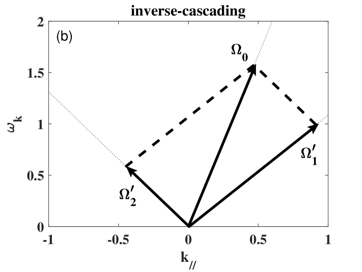
Figure 1: Sketches of frequency and parallel wavenumber matching conditions ($\omega_{k_{0}}=\omega_{k_{1}}+\omega_{k_{2}}$, $k_{\parallel 0}=k_{\parallel 1}+k_{\parallel 2}$) for (a) dual-cascading and (b) inverse-cascading KAW triplets. Black vector arrows represent the values of frequency and parallel wavenumber for each modes $\bm{\Omega}_{k}=(\omega_{k},\bm{k})$ and dashed lines constitute parallelograms for different propagation direction of $\bm{\Omega}_{2}$. The modulus of slope of each dotted line is proportional to $\alpha_{k}$, which increases monotonically with $k_{\perp}$.

IV Parametric Decay and Spectral Cascades

Considering resonant three-KAW interaction process with frequency and wavenumber matching conditions $\bm{\Omega}_{0}=\bm{\Omega}_{1}+\bm{\Omega}_{2}$ satisfied, we look into the condition for spontaneous decay, with emphasis on the energy flow among these three waves. Without loss of generality, taking $\bm{\Omega}_{0}$ as the pump wave, the frequency and parallel wavenumber matching conditions are illustrated in Fig. (1), where cases for different propagation direction of $\bm{\Omega}_{2}$ with respect to $\bm{\Omega}_{0}$ are given. It also implies the perpendicular wavenumber matching condition and embodies possible cascading behaviors in $k_{\perp}$, noting the dependence of the slope of $\omega_{k}/k_{\parallel}$ on $b_{k}$, which will be elaborated in the following analysis. Taking $\delta\phi_{k}(t)=\Phi_{k}(t)e^{-i\omega_{k}t}$ with $\Phi_{k}(t)$ being the slowly-varying amplitude, and noting $|\delta\phi_{k_{0}}|\gg|\delta\phi_{k_{1}}|,|\delta\phi_{k_{2}}|$, we obtain the linearized coupled equations

$$b_{k_{1}}\epsilon_{Ak1}\Phi_{k_{1}} = -i(\Lambda_{k_{2}}^{k_{1}}/2\omega_{k_{1}})\beta_{k_{2},k_{0}}\Phi_{k_{2}}^{*}\Phi_{k_{0}},$$ (21)

$$b_{k_{2}}\epsilon_{Ak2}\Phi_{k_{2}} = -i(\Lambda_{k_{2}}^{k_{1}}/2\omega_{k_{2}})\beta_{k_{0},k_{1}}\Phi_{k_{0}}\Phi_{k_{1}}^{*},$$ (22)

and $\Phi_{k_{0}}=\text{const}$. Expanding $\epsilon_{Ak}\simeq i\partial_{\omega_{k}}\epsilon_{Ak,r}(\partial_{t}-\gamma_{dk})$ with $\partial\epsilon_{Ak,r}/\partial\omega_{k}=2(1-\Gamma_{k})/(b_{k}\omega_{k})$, $\partial_{t}$ being the slowly temporal evolution and can be denoted as $\gamma$, and $\gamma_{dk}<0$ being the linear damping rate, we can rewrite the coupled equations as

$$(\partial_{t}-\gamma_{dk_{1}})\Phi_{k_{1}} = -\frac{\Lambda_{k_{2}}^{k_{1}}\beta_{k_{2},k_{0}}}{4(1-\Gamma_{k_{1}})}\Phi_{k_{2}}^{*}\Phi_{k_{0}},$$ (23)

$$(\partial_{t}-\gamma_{dk_{2}})\Phi_{k_{2}} = -\frac{\Lambda_{k_{2}}^{k_{1}}\beta_{k_{0},k_{1}}}{4(1-\Gamma_{k_{2}})}\Phi_{k_{0}}\Phi_{k_{1}}^{*}.$$ (24)

The resultant parametric dispersion relation is given as

$$(\partial_{t}-\gamma_{dk_{1}})(\partial_{t}-\gamma_{dk_{2}})=\frac{(\Lambda_{k_{2}}^{k_{1}})^{2}\beta_{k_{2},k_{0}}\beta_{k_{0},k_{1}}}{16(1-\Gamma_{k_{1}})(1-\Gamma_{k_{2}})}|\Phi_{k_{0}}|^{2},$$ (25)

which then yields, the condition for spontaneous decay with the $\gamma>0$

$$\gamma_{ND}^{2}\equiv\frac{(\Lambda_{k_{2}}^{k_{1}})^{2}\beta_{k_{2},k_{0}}\beta_{k_{0},k_{1}}|\Phi_{k_{0}}|^{2}}{16(1-\Gamma_{k_{1}})(1-\Gamma_{k_{2}})}>\gamma_{dk_{1}}\gamma_{dk_{2}},$$ (26)

i.e., firstly, the sign of $\beta_{k_{2},k_{0}}\beta_{k_{0},k_{1}}$ to be positive, and secondly, the nonlinear drive intensity $\gamma^{2}_{ND}$ should exceed the threshold due to linear damping of sidebands, which determines the threshold on pump KAW amplitude. Note that, the threshold could also arise from the frequency mismatch, which is, however, not considered here.

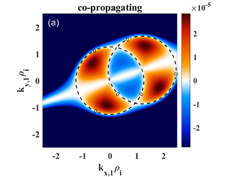
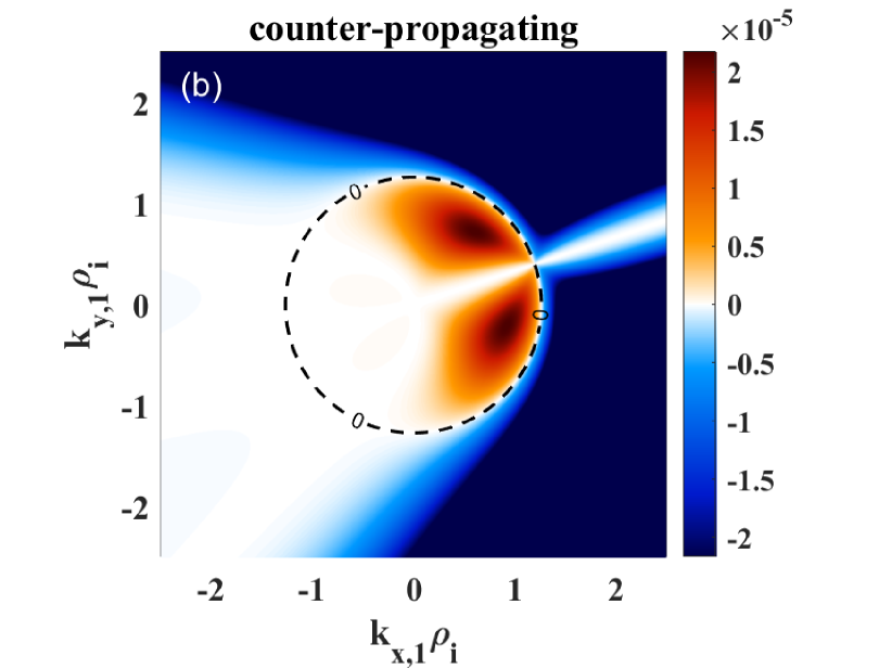
Figure 2: Intensity profiles of $\gamma_{ND}^{2}/\Omega_{i}^{2}$ for the sideband $\bm{\Omega}_{2}$ being (a) co-propagating or (b) counter-propagating. Black dashed circles represent the separatrix between positive and negative values.

The nonlinear drive $\gamma_{ND}^{2}/\Omega_{i}^{2}$ for co- and counter-propagating cases are visualized in two contour plots of Fig. 2, with the horizontal and vertical axes being $k_{x1}\rho_{i}$ and $k_{y1}\rho_{i}$, respectively. The parameter used are $\beta_{i}=0.01$, $\tau=1$, pump KAW amplitude $|\delta B_{k_{0}}/B_{0}|=10^{-3}$, and $b_{k_{0}}=1.6$ with $k_{x,0}\rho_{i}=1.2$ and $k_{y,0}\rho_{i}=0.4$. In Fig. 2, red and blue colours correspond to positive and negative values, and the boundary between stable and unstable regions are indicated by black dashed circles. For all three KAWs being co-propagating, i.e. a forward-scattering process as shown by the $(\Omega_{0},\Omega_{1},\Omega_{2})$ combination in Fig. 1, the wavenumber spectrum exhibits a dual cascading character in $k_{\perp}$, similar to that of the DW described by Charney-Hasegawa-Mima equation, which can be verified by the analytical expression $\beta_{k_{2},k_{0}}\beta_{k_{0},k_{1}}\propto(\alpha_{k_{2}}-\alpha_{k_{0}})(\alpha_{k_{0}}-\alpha_{k_{1}})$, as well as the slopes of dotted lines in Fig. 1. While for the backward-scattering process with one sideband propagating in the direction opposite to that of the pump wave, as shown by the $(\Omega_{0},\Omega_{1}^{\prime},\Omega_{2}^{\prime})$ combination in Fig. 1 or Fig. 1 (the difference is the slope of $\Omega_{2}$ with respect to the pump KAW $\Omega_{0}$), the counter-propagating KAW triplet could be manifested as either dual-cascading or inverse-cascading within the circular region in Fig. 2, which is also confirmed by the analytical expression $\beta_{k_{2},k_{0}}\beta_{k_{0},k_{1}}\propto(\alpha_{k_{0}}-\alpha_{k_{1}})$. Above preliminary cascading properties obtained from spontaneous decay condition can also be identified in Fig. (1), where the modulus of slope of each dotted line is proportional to $\alpha_{k}=\sqrt{\sigma_{k}b_{k}/(1-\Gamma_{k})}$ and thus increases with $k_{\perp}$ monotonically. Furthermore, from the contour of $\gamma_{ND}^{2}/\Omega_{i}^{2}$, we conclude that the inverse cascade is dominant for counter-propagating case, since the interval with stronger nonlinear drive falls within the region of inverse cascading ($(\Omega_{0},\Omega_{1}^{\prime},\Omega_{2}^{\prime})$ combination in Fig. 1). These different cascading behaviors in perpendicular wavenumber spectrum would further determine the stationary energy spectrum of KAW turbulence and have significant implication on cross-field transport.

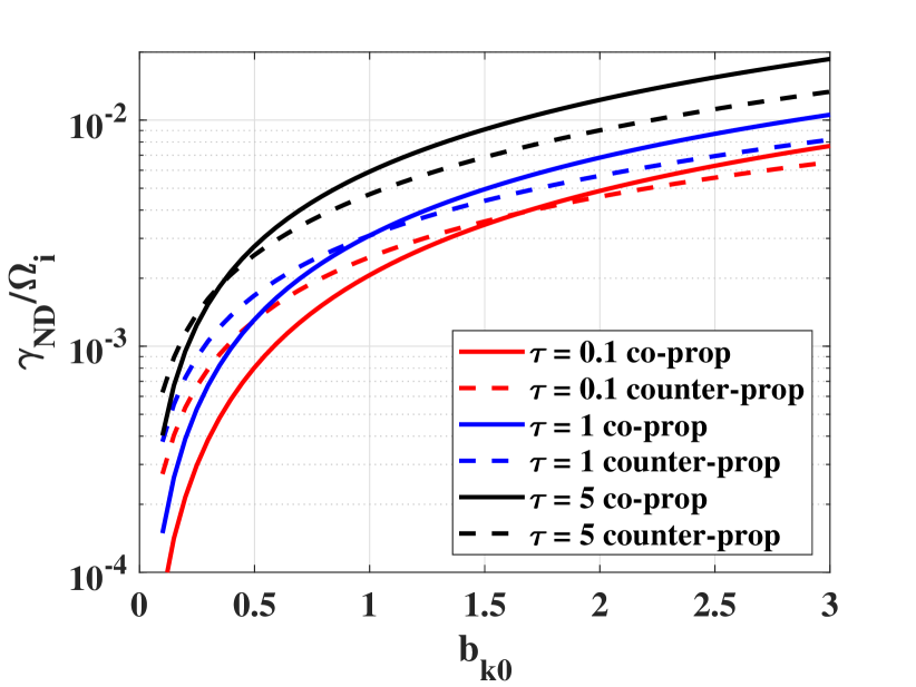
Figure 3: Parameter dependences of nonlinear drive $\gamma_{ND}/\Omega_{i}$ on $b_{k_{0}}$ for different value of $\tau$.

For different value of temperature ratio $\tau$, we can evaluate the maximized nonlinear drive $\gamma_{ND}/\Omega_{i}$ for different $b_{k_{0}}$, as shown in Fig. 3. The overall tendency is that the maximized nonlinear drive increases with $b_{k_{0}}$ monotonically. For a specific $\tau$, for relatively small $b_{k_{0}}$ decay is more effective into counter-streaming KAWs, i.e. inverse cascade in $k_{\perp}$. While in the short-wavelength region with relatively large $b_{k_{0}}$, the maximized nonlinear drive for co-propagating KAWs is slightly larger. Although the difference is not significant, the consequences on resultant saturated spectrum could be worth exploring, considering different types of cascadings.

V Conclusion and discussion

In this work, the generalized nonlinear equation governing the resonant interaction among three kinetic Alfvén waves (KAWs) in the kinetic regime with $|k_{\perp}\rho_{i}|^{2}/|\omega/\Omega_{i}|\gtrsim\mathcal{O}(1)$ is derived using nonlinear gyrokinetic equation, motivated to obtain a generalized nonlinear theoretic framework that can be applied to strongly turbulent system, with the potential application to the spectral cascading of KAWs in nature and laboratory plasmas. A generalized expression of the nonlinear coupling coefficient with concrete physics meaning is derived, which can be conveniently used for the cases with the two beating KAWs being co- or counter-propagating along the equilibrium magnetic field. The present analysis assumed uniform plasma with $\beta\ll 1$ to simplify the analysis, however, extension to more realistic parameter regimes with plasma nonuniformity accounted for should be straightforward Chen et al. (2022).

To reveal the crucial physics underlying the KAW spectral cascading, the condition for a pump KAW spontaneously decay into two sideband KAWs is analyzed. In the forward-scattering process with both sidebands being co-propagating with the pump KAW, it is found both analytically and numerically that, this corresponds to a dual cascading process in perpendicular wavenumber, similar to that of DW cascading described by the well-known Charney-Hasegawa-Mima equation. On the other hand, in the back-scattering process with one of the sidebands being counter-propagating with respect to the pump KAW, both dual- and inverse- cascading are possible, and inverse-cascading may have a larger nonlinear cross-section. These aspects can be used in later analysis for the saturated KAW spectrum with linear drive/dissipation self-consistently accounted for.

The general equation (15) for resonant interactions among KAWs, with the nonlinear coupling coefficient given by Eq. (16), is the most important result of the present work, and can be used to study the potentially strongly turbulent KAW nonlinear spectral cascading with $|\delta\omega/\omega|\sim\mathcal{O}(1)$, noting that $\omega\propto k_{\parallel}$ to the leading order for KAWs, with clear analogy to drift waves with $\omega\propto k_{\perp}$ that is imbedded in the spectral evolution described by Charney-Hasegawa-Mima equation. For further analytical progress, in the long wavelength limit with $b\ll 1$, Eq. (15) can be reduced to

$$\bm{\nabla}_{\perp}\cdot[\partial_{t}^{2}-v_{A}^{2}\rho_{i}^{2}\nabla_{\parallel}^{2}+(3/4+\tau)v_{A}^{2}\rho_{i}^{4}\nabla_{\parallel}^{2}\nabla_{\perp}^{2}]\bm{\nabla}_{\perp}\delta\phi$$

$$+(2c/B_{0})\partial_{t}[(\hat{\bm{b}}\cdot\bm{\nabla}_{\perp}\delta\phi\times\bm{\nabla}_{\perp})\nabla_{\perp}^{2}\delta\phi]=0$$ (27)

and

$$\bm{\nabla}_{\perp}\cdot[\partial_{t}^{2}-v_{A}^{2}\rho_{i}^{2}\nabla_{\parallel}^{2}+(3/4+\tau)v_{A}^{2}\rho_{i}^{4}\nabla_{\parallel}^{2}\nabla_{\perp}^{2}]\bm{\nabla}_{\perp}\delta\phi$$

$$+(3/4+\tau)(c\rho_{i}^{2}/B_{0})\partial_{t}[(\hat{\bm{b}}\cdot\bm{\nabla}_{\perp}\delta\phi\times\bm{\nabla}_{\perp})\nabla_{\perp}^{4}\delta\phi]=0$$ (28)

for counter- and co-propagating KAWs, respectively, and symmetrization has been applied in the derivation of these equations Hasegawa and Mima (1978). They are capable of describing the self-consistent turbulent evolution of KAWs with multiple Fourier modes in long-wavelength regime. It is noteworthy that, the nonlinear term for counter-propagating case is similar to that of 2D Navier-Stokes/Euler equation and Charney-Hasegawa-Mima equation, while that for co-propagating case is quite different, suggesting both quantitatively and qualitatively different cascading dynamics. Therefore, the expected conservation laws, possible vortex solutions and direct numerical simulations of turbulent evolution will be given in future works. While applying the above Eqs. (V) and (V), one needs to keep in mind that, they are derived assuming $b\ll 1$, which defines the parameter regime for their application.

As a final remark, while the interactions among KAWs are local in wavenumber space, it is expected that small-scale structures like convective cells Zonca et al. (2015) could be simultaneously excited, corresponding to zonal structures Rosenbluth and Hinton (1998); Zonca et al. (2021); Diamond et al. (2005) prevalent in fusion and atmospheric plasmas, and these important physics are not included in the present model. Taking the zonal structure generation into account, one could study the nonlinear dynamics of KAWs, including the potential implications to fusion plasmas, could be analyzed in future projects.

Author declarations

Conflict of Interest

The authors have no conflicts to disclose.

Data availability statement

The data that support the findings of this study are available from the corresponding author upon reasonable request.

References

- Alfvén (1942) H. Alfvén, Nature 150, 405 (1942).
- Hasegawa and Chen (1975) A. Hasegawa and L. Chen, Physical Review Letters 35, 370 (1975).
- Grad (1969) H. Grad, Physics Today 22, 34 (1969).
- Chen and Hasegawa (1974a) L. Chen and A. Hasegawa, The Physics of Fluids 17, 1399 (1974a).
- Hasegawa and Chen (1974) A. Hasegawa and L. Chen, Physical Review Letters 32, 454 (1974).
- Chen and Hasegawa (1974b) L. Chen and A. Hasegawa, Journal of Geophysical Research 79, 1024 (1974b).
- Chen and Hasegawa (1991) L. Chen and A. Hasegawa, Journal of Geophysical Research: Space Physics 96, 1503 (1991).
- Cranmer and Van Ballegooijen (2003) S. Cranmer and A. Van Ballegooijen, The Astrophysical Journal 594, 573 (2003).
- Sagdeev and Galeev (1969) R. Z. Sagdeev and A. A. Galeev, Nonlinear plasma theory (AW Benjamin Inc., 1969).
- Stenflo (1994) L. Stenflo, Physica Scripta 1994, 15 (1994).
- Chen and Zonca (2011) L. Chen and F. Zonca, Europhysics Letters 96, 35001 (2011).
- Hasegawa and Chen (1976) A. Hasegawa and L. Chen, The Physics of Fluids 19, 1924 (1976).
- Hasegawa and Mima (1977) A. Hasegawa and K. Mima, Physical Review Letters 39, 205 (1977).
- Hasegawa and Mima (1978) A. Hasegawa and K. Mima, The Physics of Fluids 21, 87 (1978).
- Rhines (1975) P. B. Rhines, Journal of Fluid Mechanics 69, 417 (1975).
- Hasegawa (1985) A. Hasegawa, Advances in Physics 34, 1 (1985).
- Boffetta and Ecke (2012) G. Boffetta and R. E. Ecke, Annual Review of Fluid Mechanics 44, 427 (2012).
- Kraichnan and Montgomery (1980) R. H. Kraichnan and D. Montgomery, Reports on Progress in Physics 43, 547 (1980).
- Horbury et al. (2005) T. S. Horbury, M. A. Forman, and S. Oughton, Plasma Physics and Controlled Fusion 47, B703 (2005).
- Sahraoui et al. (2009) F. Sahraoui, M. L. Goldstein, P. Robert, and Y. V. Khotyaintsev, Physical Review Letters 102, 231102 (2009).
- Salem et al. (2012) C. S. Salem, G. G. Howes, D. Sundkvist, S. D. Bale, C. C. Chaston, C. H. K. Chen, and F. S. Mozer, The Astrophysical Journal Letters 745, L9 (2012).
- Armstrong et al. (1995) J. Armstrong, B. Rickett, and S. Spangler, The Astrophysical Journal 443, 209 (1995).
- Minter and Spangler (1996) A. H. Minter and S. R. Spangler, The Astrophysical Journal 458, 194 (1996).
- Quataert (1998) E. Quataert, The Astrophysical Journal 500, 978 (1998).
- Quataert and Gruzinov (1999) E. Quataert and A. Gruzinov, The Astrophysical Journal 520, 248 (1999).
- Frisch (1995) U. Frisch, Turbulence: the legacy of AN Kolmogorov (Cambridge university press, 1995).
- Krommes (2012) J. A. Krommes, Annual Review of Fluid Mechanics 44, 175 (2012).
- Schekochihin et al. (2008) A. Schekochihin, S. Cowley, W. Dorland, G. Hammett, G. G. Howes, G. Plunk, E. Quataert, and T. Tatsuno, Plasma Physics and Controlled Fusion 50, 124024 (2008).
- Brizard and Hahm (2007) A. J. Brizard and T. S. Hahm, Reviews of Modern Physics 79, 421 (2007).
- Frieman and Chen (1982) E. Frieman and L. Chen, The Physics of Fluids 25, 502 (1982).
- Schekochihin et al. (2009) A. Schekochihin, S. Cowley, W. Dorland, G. Hammett, G. G. Howes, E. Quataert, and T. Tatsuno, The Astrophysical Journal Supplement Series 182, 310 (2009).
- Howes et al. (2006) G. G. Howes, S. C. Cowley, W. Dorland, G. W. Hammett, E. Quataert, and A. A. Schekochihin, The Astrophysical Journal 651, 590 (2006).
- Fasoli et al. (2007) A. Fasoli, C. Gormenzano, H. Berk, B. Breizman, S. Briguglio, D. Darrow, N. Gorelenkov, W. Heidbrink, A. Jaun, S. Konovalov, et al., Nuclear Fusion 47, S264 (2007).
- Chen and Zonca (2016) L. Chen and F. Zonca, Reviews of Modern Physics 88, 015008 (2016).
- Liu et al. (2022) P. Liu, X. Wei, Z. Lin, G. Brochard, G. J. Choi, W. W. Heidbrink, J. H. Nicolau, and G. R. McKee, Physical Review Letters 128, 185001 (2022).
- Liu et al. (2023) P. Liu, X. Wei, Z. Lin, G. Brochard, G. Choi, and J. Nicolau, Reviews of Modern Plasma Physics 7, 15 (2023).
- Ye et al. (2022) L. Ye, Y. Chen, and G. Fu, Nuclear Fusion 63, 026004 (2022).
- Wei et al. (2022) S. Wei, T. Wang, L. Chen, F. Zonca, and Z. Qiu, Nuclear Fusion 62, 126038 (2022).
- Todo (2018) Y. Todo, Reviews of Modern Plasma Physics 3, 1 (2018).
- Chen and Zonca (2013) L. Chen and F. Zonca, Physics of Plasmas 20 (2013).
- Chen et al. (2001) L. Chen, Z. Lin, R. B. White, and F. Zonca, Nuclear Fusion 41, 747 (2001).
- Hahm and Chen (1995) T. Hahm and L. Chen, Physical Review Letters 74, 266 (1995).
- Bale et al. (2005) S. Bale, P. Kellogg, F. Mozer, T. Horbury, and H. Reme, Physical Review Letters 94, 215002 (2005).
- Howes et al. (2008) G. Howes, W. Dorland, S. Cowley, G. Hammett, E. Quataert, A. Schekochihin, and T. Tatsuno, Physical Review Letters 100, 065004 (2008).
- Howes et al. (2011) G. G. Howes, J. M. TenBarge, W. Dorland, E. Quataert, A. A. Schekochihin, R. Numata, and T. Tatsuno, Physical Review Letters 107, 035004 (2011).
- Voitenko (1998) Y. M. Voitenko, Journal of Plasma Physics 60, 497 (1998).
- Chen et al. (2022) L. Chen, Z. Qiu, and F. Zonca, Physics of Plasmas 29 (2022).
- Zonca et al. (2015) F. Zonca, Y. Lin, and L. Chen, Europhysics Letters 112, 65001 (2015).
- Rosenbluth and Hinton (1998) M. N. Rosenbluth and F. L. Hinton, Physical Review Letters 80, 724 (1998).
- Zonca et al. (2021) F. Zonca, L. Chen, M. Falessi, and Z. Qiu, Journal of Physics: Conference Series 1785, 012005 (2021).
- Diamond et al. (2005) P. H. Diamond, S.-I. Itoh, K. Itoh, and T. S. Hahm, Plasma Physics and Controlled Fusion 47, R35 (2005).