Technical Report: Modeling Average False Positive Rates of Recycling Bloom Filters ††thanks: This material is based upon work supported by the National Science Foundation under Grant Nos. CNS-1910138, CNS-2106197, and CNS-2148275. Any opinions, findings, and conclusions or recommendations expressed in this material are those of the author(s) and do not necessarily reflect the views of the National Science Foundation.
Abstract
Bloom Filters are a space-efficient data structure used for the testing of membership in a set that errs only in the False Positive direction. However, the standard analysis that measures this False Positive rate provides a form of worst case bound that is both overly conservative for the majority of network applications that utilize Bloom Filters, and reduces accuracy by not taking into account the actual state (number of bits set) of the Bloom Filter after each arrival. In this paper, we more accurately characterize the False Positive dynamics of Bloom Filters as they are commonly used in networking applications. In particular, network applications often utilize a Bloom Filter that “recycles”: it repeatedly fills, and upon reaching a certain level of saturation, empties and fills again. In this context, it makes more sense to evaluate performance using the average False Positive rate instead of the worst case bound. We show how to efficiently compute the average False Positive rate of recycling Bloom Filter variants via renewal and Markov models. We apply our models to both the standard Bloom Filter and a “two-phase” variant, verify the accuracy of our model with simulations, and find that the previous analysis’ worst-case formulation leads to up to a 30% reduction in the efficiency of Bloom Filter when applied in network applications, while two-phase overhead diminishes as the needed False Positive rate is tightened.
Index Terms:
Bloom Filter, False PositivesI Introduction
Bloom Filters [3] are a time-tested, space-efficient data structure for identifying duplicate items within an input sequence, and have been applied in an extremely broad set of computing applications, including packet processing and forwarding/routing in P2P networks [19], cache summarization and cache filtering in CDNs [13], network monitoring [9], data synchronization [12], and even Biometric authentication [15]. The Bloom Filter (BF) is attractive because it errs only in the False Positive direction (an arriving input, which we call a message, can be incorrectly identified as a repeat of a previous message) and never the False Negative direction (a repeat message is never incorrectly classified as new).
There are several variants of “back-of-the-envelope” analyses111Later in the paper, we look at different variants. that give the False Positive rate of an st message after messages have been inserted, e.g., one common variant yields , where is the memory (number of bits in the BF) and is the number of hash functions, with each hash function mapping the message to one of the bits. This analysis, while useful to demonstrate efficacy of the BF, does not measure False Positives in a way that best serves practical network applications for two reasons:
Observability: First, consider the addition of an th element. If the application maintains a count, , of the number of bits set, the next new arrival being classified as a repeat (a False Positive) can be directly computed as ; the earlier analysis disregards the ability to inspect current BF state.
Average rate: Second, the False Positive rate of a newly arriving message grows as the BF’s number of set bits increases. Because of this, applications that merely wish to bound the average False Positive rate across all newly arriving messages significantly overestimate this average rate when only considering the message with the worst case bound.
A class of applications that would benefit from a measure of False Positive rate that takes into account both observability and average rate are those that employ what we call a Recycling Bloom Filter (RBF) [13, 20, 16]. These applications utilize BF’s across sufficiently long timescales, where new messages are continuously arriving, but are interspersed with repeats of previous messages. Since newly arriving messages almost always set bits in the BF, over time the number of bits will become excessive, driving up the False Positive rate, such that some bits must be cleared to keep False Positive rates at a reasonable level. While there are BF variants that do support deletion, their implementation introduces substantial overhead or requires knowledge of the specific elements destined for deletion [17, 10, 7, 2]. Such overhead and complexity is not suited for network applications where message arrivals have a “fading popularity” character, with repeat probability decreasing over time. For applications with this type of message arrival process, one can utilize an active metric that maintains some measure of BF fullness, such as the number of messages inserted, or the number of bits set in the BF. When this metric exceeds a threshold, the BF recycles: all bits are cleared, and the filling process begins anew (we say a new BF cycle is initiated). This process can continue indefinitely, providing a simple and effective means for maintaining a low maximal (and average) False Positive rate of arrivals.
In this paper, we develop recursive, quickly computable (on today’s conventional hardware) analytical models that accurately capture the average False Positive rates of Recycling BFs (RBFs). We show that using an active metric to gauge the recycle to maintain an average (as opposed to maximum) False Positive rate can offer a % or more increase in amount of messages stored.
While the recycling process does introduce the possibility of False Negatives, the aforementioned decline in popularity of each message over time ensures that well-provisioned RBFs can make False Negative rates negligible. While a detailed investigation of False Negatives is beyond the scope of this paper, a commonly used solution ([13], [20]) to further drive down False Negative rate is to implement what we refer to as a two-phase RBF (see IV-F1 for details) that splits the memory between alternately active and “frozen” BFs. We extend our models to analyze these two-phase variants, and measure the loss in efficiency of minimizing False Positive rate as a function of memory and expected number of messages stored in the BF.
In this paper, we make the following contributions:
Our findings show that the variant that recycles based on the number of bits set, while most complex to model to find the right parameters, is the best performing variant in that it can maintain a given False Positive rate while packing in the largest expected number of messages prior to recycling. In contrast, the variants that recycle based on message counts to achieve an average False Positive rate are easier to model and achieve only a slightly smaller expected number of messages prior to recycling. These average-case variants store around 30% more messages in expectation than the commonly used worst case variant. We also find that implementing a two-phase variant will closely match the one-phase as the False Positive rate to be met decreases. These results are important in that they point to users of BFs (and specifically RBFs) likely being overly conservative for their needs when using previous measures of False Positives.
II Background
| Variable | Description |
|---|---|
| Model input parameters | |
| Size of RBF (bits) | |
| Number of hash functions per message | |
| RBF recycle point (number of new message arrivals) | |
| RBF recycle point (number of bits set) | |
| Markov Model internal variables | |
| Probability next arrival takes RBF from to bits | |
| * is one of | |
| Steady-state probability RBF contains bits set | |
| False Positive Variants | |
| False Positive rate using worst-case threshold (1) | |
| False Positive rate using fixed oracle lower bound (2) | |
| f.p. rate using fixed bit-setting msgs lower bound (3) | |
| False Positive rate using bound (# bits set ), | |
| one-phase RBF (18) | |
| False Positive rate using bound, two-phase RBF (26) | |
II-A Bloom Filters
A Bloom Filter [3] can be thought of as an array of bits indexed , all initially set to , that uses hash functions, each of which maps an arriving message to a bit in the array: the bit is then set to 1. Importantly, these hash functions’ mappings are independent across messages, such that each message’s assignment of bits is effectively independent from those assigned to other messages. This independence property is what makes the BF such a powerful abstraction, as well as amenable to mathematical analysis.
When a message arrives, the bits to which it hashes are checked before being set. If they are all already set, the message is assumed to be a repeat of a prior message. In the rare instance that a new message’s hashes point to bits already set, it is incorrectly classified as a repeat, i.e., a False Positive.
II-A1 Colliding vs. Non-Colliding Hash Functions
Conventional implementations of hash functions permit several of the hash function mappings to collide and hash to the same bit (i.e., a pseudo-random sampling with replacement). A slightly more sophisticated hashing scheme can ensure the hashes for a message are distinct from one another (i.e., a pseudo-random sampling without replacement). We respectively refer to these two Bloom Filter variants as colliding and non-colliding, and we analyze both types. While we show how to incorporate these variants into our models, for values of and used in practice (typically ), the colliding/non-colliding distinction has an unnoticeable impact on False Positive rate (collisions are sufficiently rare in the colliding variant). Note that for either variant of hash functions, the independence of bits assigned to differing messages still holds. Hence, our results are generally presented using the colliding variant.
II-B Traditional False Positive Analysis
As discussed in §I, after having received unique messages, the (colliding) False Positive likelihood of the st message is
| (1) |
where, for a given and , will minimize the corresponding False Positive rate. Wikipedia provides a succinct derivation of this simple formula [21], as well as a formula for non-colliding hash functions (in terms of Stirling numbers). From (1), the False Positive rate approaches as the number of messages increases– an undesirable property for applications with no limit on the number of potential message insertions. We call using such a bound in practice to decide when to recycle the BF a worst case bound (hence ) because the recycling occurs as soon as a particular message’s False Positive rate exceeds (while the average over messages inserted will be lower). We refer to the lifetime of a BF between recycling events as a cycle of the BF.
II-C Two-Phased Bloom Filter
An RBF, upon recycling, clears all memory with respect to previous arrivals. To mitigate the effects of this memory loss, a BF variant called a Two-Phase Bloom Filter has been used in various network applications, e.g., [13, 20].
The two-phase Bloom Filter can be thought of as two arrays with bits each, indexed , along with independent hash functions that are shared across both arrays. Typically, , where is what the application’s memory constraint would be for the standard (one phase) Bloom Filter.
The two-phase variant operates much like the standard recycling variant, with the addition that at any point in time, one Filter array is designated active and the other frozen. Incoming messages are hashed and added to the active filter. When the active filter is considered to be “full enough” (e.g., the number of bits set or messages stored exceeds some threshold), instead of clearing the bits of the active filter, we clear the bits of the frozen filter. The roles of the active and frozen filter are then switched; incoming messages are added to the previously frozen (now active) filter, and the status of the previously active (now frozen) filter remains unaffected. This process repeats indefinitely.
In the two-phase variant, an arriving message is hashed and its bits are compared separately within both the active and frozen filters. A match with either filter is interpreted as the message having been received previously (and having set the corresponding bits in the respective filter). While a two-phase RBF cannot reduce its false positive rate as effectively as its one-phase counterpart using identical total memory, its corresponding False Negative rates will often be significantly lower.
II-D BF Thresholding Approaches
There are two basic approaches to deciding when to recycle a BF. One can count the number of bits that are set in the BF and recycle when exceeds a threshold . We call this approach a -bounded approach. Alternatively, one can bound the number of bit-setting messages, , that can be admitted into the BF before recycling.222Messages that don’t set bits are generally not counted because the user must assume they are repeat messages, and since repeat messages never set bits, the False Positive rate of the BF does not increase due to their repeated arrival. We call this approach an -bounded approach. We note that one complication with an -bounded approach is that when a message that arrives without setting any bits, a user cannot tell if it is a repeat message or a False Positive. A drawback of formulas for an -bounded approach, such as (1), is that they count new messages regardless of whether or not new bits are set; since in practice new messages that do not set bits are assumed to be repeats, a user will underestimate the number of new messages received when False Positives occur, such that applications of a formula such as (1) to gauge when to recycle will be slightly off.
II-E Averaging Variants
A BF is only of use when the message arrival process consists both of new and repeat messages. We wish to clarify a subtle point about what we are averaging over. When a message first arrives, if it sets additional bits, it is identified as new, and if not, it is classified as a repeat. Consider the th new message that arrives, and let represent the number of times the message arrives within a cycle, and let be an indicator that equals 1 if the th message, upon first arrival, is a False Positive. We can count these arrivals in three different ways.
-
1.
count-first: We can assume that only the first arrival can count as a False Positive, making the False Positive rate for the cycle equal to
-
2.
count-each: We can assume that each arrival of a message that initially triggered a False Positive is counted as a False Positive, making the False Positive rate equal to
-
3.
count-instance: We only measure the False Positive rate of first-time arrivals of a message, making the False Positive rate equal to
Which variant to use depends on the needs of the underlying application. For instance, a False Positive in a caching application that uses the BF to determine cache hits for requests would make the wrong assessment for an initial arrival of a request, but the mistake would be detected upon attempting to fetch the item from the cache, so the item would be cached and subsequent requests would not be false positives. Hence, count-first is the appropriate measure. Alternatively, a mechanism that wishes to count unique messages would have a single miscount for each message initially classified incorrectly as having been previously received, hence count-instance is the appropriate measure. Finally, in a setting where the BF is used to drop repeat requests, and where a penalty is paid per dropping of an unsatisfied request, count-each would be the appropriate measure.
We can prove that count-instance is the most stringent (largest) of False Positive rates of the three versions333count-first is straightforwardly smaller count-each.. The proof showing that count-instance results in the largest False Positive rate is omitted here but is included in §-A in the Appendix. This observation yields two benefits. First, if we compute the false positive rate for count-instance, we have upper bounds on the rates of the count-first and count-each variants.444In fact, our analysis of count-instance is itself an upper-bound in an RBF for a subtle reason that we address in the extended version. Second, count-instance is not affected by underlying distribution of arriving messages: how often a particular message repeats is of no import, since we only decide its contribution to False Positive rate based on its first arrival, and any subsequent arrivals do not alter the bits in the BF, making its analysis identical regardless of this underlying distribution, whereas the other variants do depend on the underlying distribution.
The remainder of this paper utilizes count-instance, i.e., the False Positive rate is defined with respect to how new arrivals are classified upon their arrival, as it is the most stringent of the three, and provides an upper bound on the other interpretations of false-positive rate.
III -bounded average False Positive rate
We compute a lower bound on the -bounded average False Positive rate that utilizes the formula which determines worst-case False Positive rate (i.e., (1) for colliding hash functions). Define to be an indicator r.v. that equals 1 when the th new arrival is a False Positive. Note that is solved directly by worst-case bound formula (1) directly.
First, let us consider an oracle user, who, when inserting a message that sets no bits, can distinguish whether this message is a repeat, or a new message that failed to set bits.555This oracle is a hypothetical user because the user can make such a distinction has no need for a BF. This oracle would insert exactly new messages, and the resulting average False Positive rate can be computed as a simple renewal process, yielding a count-instance oracle -bounded average False Positive rate of:
| (2) |
In contrast, a “real” user would assume that a new message that sets no bits is instead a repeat message, and would not include such a message in their count of messages. Hence, the oracle would recycle no later than an actual user, thereby ensuring a lower false positive rate. For this real user, we let iterate over the number of new messages that set bits, and define r.v. to equal the number of new messages that do not set bits and arrive between the st and th new messages that do set bits. Then for a single cycle of the RBF, the False Positive rate is .
Note that for the messages that comprise a given , the number of bits set in the BF remains constant (none of the messages are changing the number of bits set), so each such message has an equal likelihood, which we call , of not setting additional bits. Note it follows that , such that . By renewal theory, we have the False Positive rate is thus equal to
Finally, we show that is lower-bounded by . This follows from the fact that the th new message that set bits is actually the th arriving message with , so for some . The lower bound then follows from the fact that is increasing in (False Positive rates increase as more messages arrive), and that the worst-case analyses’ value for is over all messages, including those that set no bits. Hence, for . Since we are underestimating each , we are underestimating the likelihood of new arrivals not setting bits, so we are underestimating False Positive rates. Note that for low False Positive rates that are used in practice, will tend to be very small, such that the bound is expected to be tight.
It will be useful for our purposes to define, for and directly applying (1), a lower bound on the -bounded False Positive rate of
| (3) |
We refer to this as the average-case N lower bound. Note that these lower-bound the False Positive rate as a function of . In §V, we use these formulae to determine as a function of False Positive rate: since the formula gives a lower bound on the False Positive rate for a given , it indicates an upper bound on the value of needed to ensure (lower-bound) a given False Positive rate.
IV -bounded average False Positive rate
As a starting point towards developing a recursive analytical model that accurately captures the average False Positive rates for the -bounded model, we consider a process where messages sequentially arrive at the RBF. Once a message arrives, the hash functions are applied to it and the corresponding bits are set to (or remain if already set). In a departure from the -bounded method of Bloom Filter recycling, we do not reset the RBF after unique message insertions. Instead, we have a predetermined bit capacity parameter . After the insertion of a message, let be the number of bits set to 1 in the RBF. We reset the RBF when . Our recursive Markov Model will allow us to determine the long-term average False Positive rate across all new arrivals for a given value of (another departure from the traditional False Positive analysis, which only considers the “worst case” False Positive rate for the last arrival of a RBF reset cycle).
IV-A RBF Recursive Markov Model
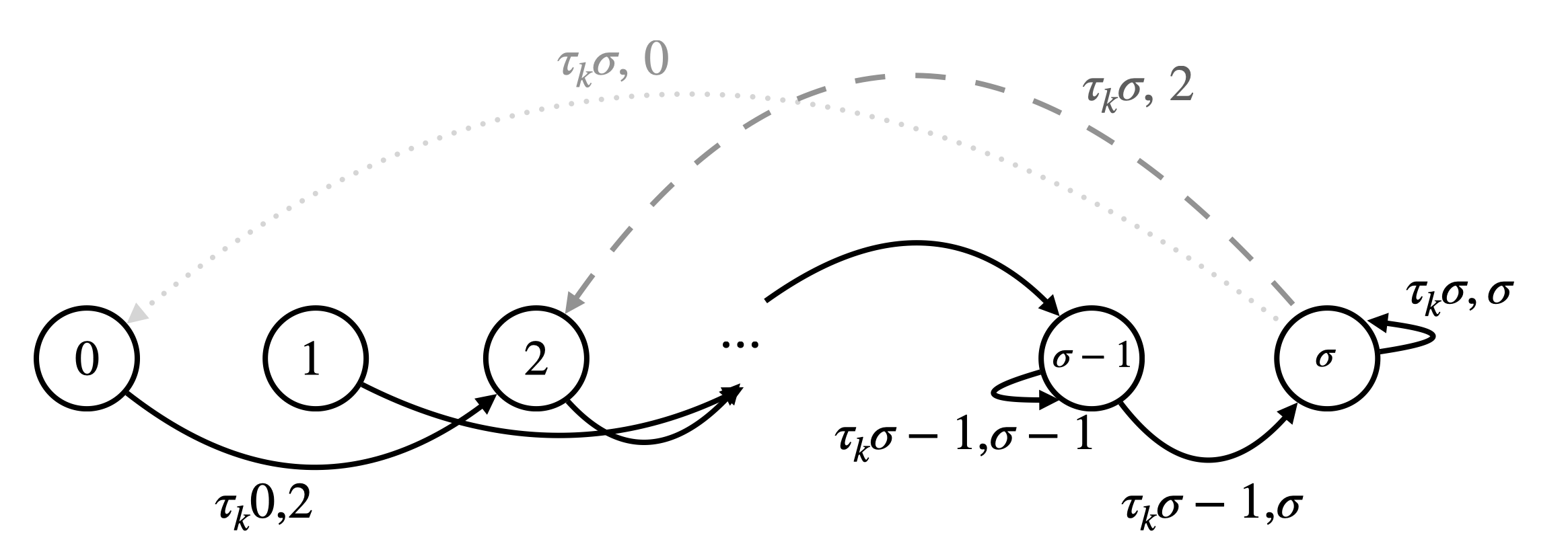
Our Markov Model for the dynamics of the RBF has states labeled . The state labels correspond to the number of bits set to in the RBF during a given cycle. After the arrival of a unique message (i.e., not yet seen this cycle), depending on the outcome of the hash operation, the number of set bits in the RBF may or may not change. We represent this event by transition probabilities between the states, labeled . The number of employed hash functions, , determines which transition probabilities are nonzero– e.g. from state , the “largest” possible state we can transition to is state . A partial diagram of our Markov Model, displaying only the “forward” transition behavior, is shown in Fig. 1.
IV-B Retaining vs. Non-Retaining RBF
We model the resetting of the RBF with “backwards” transition probabilities from certain states to earlier states . In practice, RBFs can implement recycling behavior in two ways: if message causes the RBF to reset (, after clearing all the bits, we can:
-
i
Retain message and re-insert it as the first message for the new RBF cycle
-
ii
Forget message and have the next arrival as the first message for the new RBF cycle
We call (i) the retaining version of the RBF and (ii) the nonretaining version. For both the retaining and non-retaining RBF, nonzero backwards transition probabilities exist at states . For the retaining RBF, the backwards transitions are to states . For the non-retaining RBF, all backwards transitions are to state . While we analyze both versions, the non-retaining version is slightly simpler for analysis purposes and is the version we work with unless otherwise mentioned. Fig. 2 shows a partial diagram of our Markov Model displaying the backward transitions.
IV-C RBF Long-Term Average False Positive Rate
With our Markov Model specified, we can derive an expression for the long-term average False Positive Rate of the RBF, for both colliding and non-colliding BFs, and also derive the backward transitions for colliding/noncolliding and retaining/non-retaining versions (four in total).
IV-C1 Transition Probabilities
We start by deriving expressions for the forward transition probabilities of an arriving (new message), where is the number of hash functions, is the number of bits set to 1 in the BF prior to insertion of the arriving message, and is the ending number of bits set to 1 (after the next message is hashed into the filter). We accomplish this for forward transitions from to by recursively defining in terms of and . The explicit recursive equation depends upon whether the BF is being implemented using colliding (vs. non-colliding) hash functions, as well as whether it is retaining (vs. non-retaining). The intuition behind the recursion is that the th hash function will add at most one bit in the BF after the other hashes have been applied. The BF transitions from to bits being set if either a) the first hashes transition to bits and the last hash is to a bit previously set (by earlier messages and/or the preceding hashes of the current message), or b) the first hashes transition to bits set, and the last hash maps to an unset bit. Note that these recursive equations make use of the independence properties of the hash functions applied within Bloom Filters; each message’s hashes are independent of those of previous hashes, colliding hashes for a given message are also independent from one another, and non-colliding hashes are chosen via sampling without replacement. The former property ensures that a message arriving to a BF with bits set can assume these bits were simply sampled uniformly at random.
We define to be the transition probability when the BF uses colliding hash functions and is non-retaining. In this case when :
| (4) |
| (5) |
And the base case relations:
| (6) | |||||
| (7) | |||||
| (8) |
where is an indicator that equals 1 when is true, and is otherwise 0. For colliding + retaining, denote as . has identical form to equation (4) for . We also have:
| (9) |
| (10) |
IV-C2 Steady-state Probabilities
For our Markov Model, let us denote by the steady-state probability the RBF has bits set, where (this is equivalent to the probability of the Markov chain being in state ).
For both the colliding + non-retaining / non-colliding + non-retaining versions of the RBF, the Markov Chain is clearly ergodic. Therefore the stationary distribution can be computed by solving for :
| (15) |
We can solve the equations for all by starting with an arbitrary positive assignment (a “guess”) for ; call this . Then, we apply (12) to recursively compute for as functions of . Since the sum over all steady state probabilities must be 1, we can renormalize each .
For the steady-state probabilities of the non-colliding, non-retaining version of the RBF, we can apply an identical method as above, except we have for . Thus, we make our initial “guess” for the steady-state probability , but the sets of equations are otherwise unaltered from the previous case.
For the steady-state probabilities of the colliding, retaining version of the RBF, we have an additional complexity. Equation (12) now holds only for . For , due to the backwards transitions to these states, the steady-state probabilities are given by:
| (16) |
To solve for the set of , we can take the set of equations of (12) and (13), along with the constraint , and solve by standard linear methods.
IV-C3 Expression for Long-Term Average False Positive Rate
Let us denote by the long-term average False Positive rate when in state .
For both the colliding and non-colliding versions of the RBF, we have:
| (17) |
Then the overall long-term average False Positive rate for the RBF is given by (using the desired definition of from (17):
| (18) |
IV-D Closed-Form expression for
For the case of colliding, non-retaining, and , we can explicitly solve the above expressions in closed form for the , yielding a closed form expression for the false long-term average False Positive rate:
| (19) |
IV-E Computational Complexity of Calculations
Our computation proceeds with an outer-most loop iterating over , with only when and is otherwise 0. For the next value of , we compute for values of and ranging between 0 and . Noting that for (hashing to bins cannot set more than bits), this involves total computations, making the overall time complexity of . If only one value of is being evaluated, it is possible to produce the table of all necessary holding only values, so it can also be done efficiently in memory.
Once the requisite have all been computed, computing the steady-state probabilities for the non-retaining case can be done in time, since there are a total of steady-state probabilities () and each of them involve a sum across terms.
Computing the steady-state probabilities for the retaining case can be done in time. There are a total of steady-state probabilities (), and corresponding equations for . Each of these equations contain terms; linearly combining a pair of rows is therefore an operation. Thus, with row reductions, each with complexity , we can compute for all (total complexity . We can subsequently compute for directly from (16); this takes time, so the row reduction step is the complexity bottleneck.
Computing the long-term average RBF False Positive rate as in (18) can be done in time for colliding and time for non-colliding (using the fact that to compute the terms in constant time).
Since the long-term average RBF False Positive rate is computed by successive and separate (but dependent) computations each upper-bounded by , the overall computational complexity is .
IV-F Expected messages within a -bounded RBF
In each cycle of a -bounded RBF, the number of messages that are hashed into the BF prior to recycling will vary, depending on the number of hash collisions between (and for colliding, also within) messages. We conclude our analysis of the one-phase BF by showing how the expected number of messages can be computed.
Consider a particular sample path (i.e., cycle) of the RBF, and let indicate the number of bits set after the arrival of the th new message. Let equal the number of additional messages sent after the th message to trigger a recycle (i.e., cross the sigma threshold). Note that when , we have already crossed the threshold such that . Otherwise, when , more messages must be received, such that
where is an indicator that equals 1 only when additional bits get set from the arrival of the th message.
Noting the above equation holds irrespective of the value of , we can simply replace with and just write , which we replace with to get the result . We can similarly substitute in the r.v. for which indicates that this st message takes the BF from having bits set to . This can be solved to permit a reverse recursion:
| (20) | |||||
| (21) |
Noting independence of the from , and that , we can rephrase the above as an expectation:
| (22) | |||||
| (23) |
and our solution is simply .
IV-F1 Two-Phase RBF Long-term average False Positive Rate
We can use the results from the standard RBF to also derive an expression for the False Positive rate of the two-phase RBF variant. Let denote the steady-state probability of the frozen filter having bits. Note is only nonzero for between and . To compute , we first define an un-conditional (non-normalized) value of to then compute a normalized (conditional) version of in terms of :
| (24) | |||||
| (25) |
The long-term average False Positive rate for the two-phase RBF is then given by the expression (using the desired definition of from (17):
| (26) |
V Results
To evaluate our models and draw conclusions about the performance of the RBF under varying parameters, we proceed in three steps:
-
1.
We verify the accuracy of our models through discrete event-driven simulations implemented in Python. The RBF data structures were implemented using standard Python libraries. The uniform hash function generation and random message arrival process leveraged the Python random library. Code can be found at: [1]
-
2.
With the accuracy of the models verified, we turn to the question of the maximum message capacity achievable by a RBF while staying below a given False Positive rate. We consider four models of a one-phase RBF: the -bounded model (18), the “oracle” -bounded False Positive rate (2), the lower-bound on the -bounded average False Positive rate, (3), and the traditional worst-case bound (1). The -bounded model maintains the highest number of messages, followed by , , and the lowest. This sequence implies that -bounding variants are overly conservative estimates. Therefore, if one aims to size a RBF to achieve the best performance, the -bounded variant should be utilized.
-
3.
Finally, for the -bounded model, we investigate the trade-off between using a one-phase and two-phase RBF variant, in terms of the maximum memory capacity achievable by each variant while staying below a given False Positive rate.
We note that the results for the combinations of colliding/non-colliding and retaining/non-retaining variants are nearly identical, and thus for brevity all graphs represent the colliding/non-retaining combination.
V-A Verification of Model Accuracy
V-A1 One and Two-Phase Sigma Bound
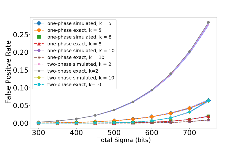
We verify the accuracy of and through discrete event-driven simulations. For all simulations, we have a fixed RBF size of bits. The two-phase RBF splits this memory evenly between each filter. We run multiple simulation epochs of message arrivals, recording the average False Positive rate at the end of each epoch. Message arrivals are drawn uniformly from a pre-generated distribution of messages. Given a collection of average False Positive rates, we can plot sample means and confidence intervals using standard statistical methods [18]. We compare these results to the values predicted by and . Fig. 3 depicts the results. We simulated for a total of epochs for and epochs for . The % confidence interval is indicated on the plot by the shaded area around the simulation curves. For all data points, the value of and lies within the confidence interval. This is strong evidence in favor of the accuracy of and in modelling False Positive rates for RBFs.
V-A2 Lower bounds on False Positive rate
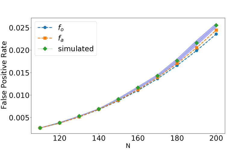
We turn next to verifying the accuracy of and . For this, we ran simulation epochs of messages each. Fig. 4 shows the simulation results plotted against and , with the % confidence interval shown. For all data points, both and are below the sample mean, and fall either within or below the confidence interval. This demonstrates strong evidence in favor of the accuracy of the lower bounds . Observe that is a “tighter” lower lower bound than .
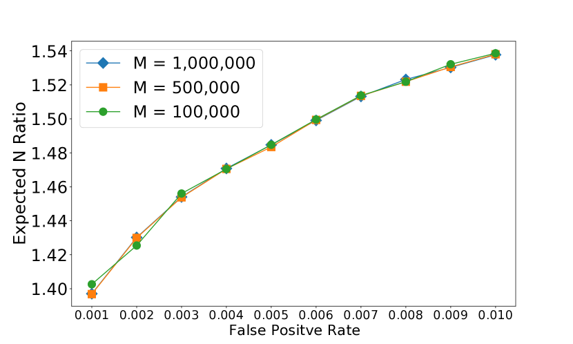
V-B Expected Message Capacity Comparison
A natural question to ask when optimizing RBF parameters is the expected maximum number of messages one can store while staying under an acceptable average False Positive rate– we refer to this as the expected message capacity. For the one-phase -bounded model (False Positive rate given by ), recall this is derived in §IV-F. We can also compute an expected message capacity using or . Fig. 5 compares the expected message capacity between the three models. For each model, we fix an average False Positive rate of . For each value of , we find the maximum number of messages subject to the False Positive constraint. We plot this number normalized to , as this is the model that yields the highest message capacity. is seen to be a good approximation, a direct consequence of the tightness of the lower bounds discussed in §III. Observe that can lead to an overly conservative estimate of message capacity in this context; for the given parameters its maximum message capacity is consistently reduced by more than 30%.
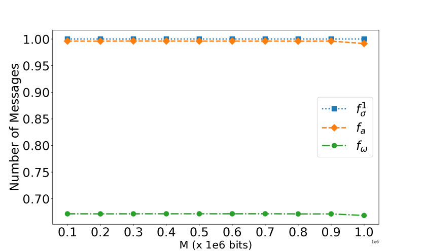
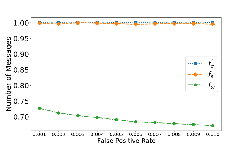
Fig. 6. shows similar results, this time varying False Positive rates on the x-axis. Once again, the worst-case model sees a consistent underestimation of maximum message capacity of around %.
We can easily conclude that, for applications that are more concerned with average False Positive rates than worst-case ones, not an ideal metric, as compared to or .
V-C Tradeoff between One and Two-phased RBF
In Fig. 7, we compare the False Positive rates of one-phase RBFs () versus their two-phase counterparts (). We have a given filter memory (which in the case of the two-phase RBF is split evenly between both filters) and False Positive rate. We then find the value of which allows us the maximum number of expected messages for these constraints. In both cases, we observe the result that the one-phase RBF appears to outperform the two-phased filter when it comes to squeezing out extra filter bit capacity. One might be moved to ponder what is the point of the added complexity of a two-phased filter, if it apparently is “less efficient” in terms of average False Positive rate? The answer becomes apparent when we consider the idea of False Negatives as we previously mentioned. While a detailed investigation of False Negatives is beyond the scope of this paper, the intuition is that the extra bit capacity seemingly afforded by the one-phase filter comes with an increased probability of False Negative rates, which are mitigated by the two-phase filter.
VI Related Work
Luo et al. provides a general summary of Bloom Filters and their variants, along with their applications to problems in computing [11]. To the best of our knowledge, all previous analyses of Bloom Filters approach the question of False Positive rates from the perspective of a “worst case” bound. Equation (1) is widely used in most applications to compute the False Positive rate according to this metric. Two prior works have shown this equation is slightly inaccurate, and in fact a lower bound for the true “worst case” False Positive rate [4, 5].
There have been other BF variants proposed that consider the need to periodically remove items from the filter. The Counting Bloom Filter (CBF) [8] and similar variants support deletion of individual elements. However, the CBF and its variants all come with increased space and algorithmic overhead to support deletion. Among similar lines, variants such as the Deletable Bloom Filter [17], the Ternary Bloom Filter [10] and the Quotient Filter [2] support element deletion under restricted circumstances, also at the cost of increased space and algorithmic complexity.
The idea of periodically resetting a targeted subset of BF bits is first proposed in Donnet et al. [6]; while this method is shown to reduce the overall False Positive rate, it also comes at the cost of increased algorithmic complexity. More recently, Cuckoo Filters have been used as an extension of Bloom filters. Cuckoo filters use Cuckoo hashing to optimize space utilization. These filters notably offer the ability to delete elements post-insertion without practical overhead [7]. However, this requires knowledge of the elements that necessitate deletion, a condition not commonly met in many networking applications. In addition, unlike RBFs, Cuckoo filters possess a finite unique message capacity. This inherently limits the scope of its usage under conditions where an unknown and continuous influx of elements is anticipated, which are common in many networking applications.
Many applications employ the RBF strategy as a low-cost alternative to deal with the need to remove elements periodically. Akamai deploys a two-phase RBF approach to guarantee that any content that ends up being cached in their edge servers has been requested at least twice within a designated time frame [13]. Bloom Filter Routing (BFR) has also been introduced in Information-Centric Networks (ICN) to simplify the process of content discovery across the networks [14] and in wireless networking where Trindade et al. have designed Time Aware Bloom Filter to only remove specific bits that have not been “hit” during a predefined time window [20].
VII Conclusion
Bloom Filters and their variants are a space-efficient data structure employed widely in all manner of computing applications. Their space efficiency comes with the tradeoff of potential False Positives, and as such much work has been dedicated towards detailed False Positive analysis. Yet all this work approaches the question of False Positives from the perspective of a “worst-case” bound. This bound is overly conservative for the majority of applications that use Bloom Filters, as it does not take into account the actual state of the Bloom Filter after each arrival. In fact, applications that use Bloom Filters often have to periodically “recycle” the filter once an allowable number of messages threshold has been exceeded. In cases such as these, different metrics such as the long-term average False Positive rates across new arrivals may be of more interest than a worst-case bound.
We derive a method to efficiently compute the long-term average False Positive rate of a Bloom Filter that periodically “recycles” itself (termed a Recycling Bloom Filter). We use renewal and Markov models to respectively derive lower bound exact expressions for the long-term average False Positive rates, and apply our model to the standard Recycling Bloom Filter, and a “two-phase” variant that is popular in network applications. We demonstrate that the previous worst-case analysis of False Positives can lead to a reduction in the efficiency of RBFs in certain scenarios.
References
- [1] https://github.com/kadzier/Recycling-Bloom-Filters-False-Positives.
- [2] M. A. Bender, M. Farach-Colton, R. Johnson, R. Kraner, B. C. Kuszmaul, D. Medjedovic, P. Montes, P. Shetty, R. P. Spillane, and E. Zadok. Don’t thrash: How to cache your hash on flash. Proc. VLDB Endow., 5(11):1627–1637, jul 2012.
- [3] B. H. Bloom. Space/time trade-offs in hash coding with allowable errors. Communications of the ACM, 13(7):422–426, 1970.
- [4] P. Bose, H. Guo, E. Kranakis, A. Maheshwari, P. Morin, J. Morrison, M. Smid, and Y. Tang. On the false-positive rate of bloom filters. Information Processing Letters, 108(4):210–213, 2008.
- [5] K. Christensen, A. Roginsky, and M. Jimeno. A new analysis of the false positive rate of a bloom filter. Information Processing Letters, 110(21):944–949, 2010.
- [6] B. Donnet, B. Baynat, and T. Friedman. Retouched bloom filters: allowing networked applications to trade off selected false positives against false negatives. In Proceedings of the 2006 ACM CoNEXT conference, pages 1–12, 2006.
- [7] B. Fan, D. G. Andersen, M. Kaminsky, and M. D. Mitzenmacher. Cuckoo filter: Practically better than bloom. In Proceedings of the 10th ACM International on Conference on emerging Networking Experiments and Technologies, pages 75–88, 2014.
- [8] L. Fan, P. Cao, J. Almeida, and A. Broder. Summary cache: a scalable wide-area web cache sharing protocol. IEEE/ACM Transactions on Networking, 8(3):281–293, 2000.
- [9] Y. Li, R. Miao, C. Kim, and M. Yu. FlowRadar: A better NetFlow for data centers. In 13th USENIX symposium on networked systems design and implementation (NSDI 16), pages 311–324, 2016.
- [10] H. Lim, J. Lee, H. Byun, and C. Yim. Ternary bloom filter replacing counting bloom filter. IEEE Communications Letters, 21(2):278–281, 2016.
- [11] L. Luo, D. Guo, R. T. Ma, O. Rottenstreich, and X. Luo. Optimizing bloom filter: Challenges, solutions, and comparisons. IEEE Communications Surveys & Tutorials, 21(2):1912–1949, 2018.
- [12] L. Luo, D. Guo, J. Wu, O. Rottenstreich, Q. He, Y. Qin, and X. Luo. Efficient multiset synchronization. IEEE/ACM Transactions on Networking, 25(2):1190–1205, 2017.
- [13] B. M. Maggs and R. K. Sitaraman. Algorithmic nuggets in content delivery. ACM SIGCOMM Computer Communication Review, 45(3):52–66, 2015.
- [14] A. Marandi, T. Braun, K. Salamatian, and N. Thomos. Bfr: A bloom filter-based routing approach for information-centric networks. In 2017 IFIP Networking Conference (IFIP Networking) and Workshops, pages 1–9, 2017.
- [15] E. Martiri, M. Gomez-Barrero, B. Yang, and C. Busch. Biometric template protection based on bloom filters and honey templates. Iet Biometrics, 6(1):19–26, 2017.
- [16] L. McHale, J. Casey, P. V. Gratz, and A. Sprintson. Stochastic pre-classification for sdn data plane matching. In 2014 IEEE 22nd International Conference on Network Protocols, pages 596–602. IEEE, 2014.
- [17] C. E. Rothenberg, C. A. Macapuna, F. L. Verdi, and M. F. Magalhaes. The deletable bloom filter: a new member of the bloom family. IEEE Communications Letters, 14(6):557–559, 2010.
- [18] K. Sidik and J. N. Jonkman. A simple confidence interval for meta-analysis. Statistics in medicine, 21(21):3153–3159, 2002.
- [19] S. Tarkoma, C. E. Rothenberg, and E. Lagerspetz. Theory and practice of bloom filters for distributed systems. IEEE Communications Surveys & Tutorials, 14(1):131–155, 2012.
- [20] J. Trindade and T. Vazão. Hran-a scalable routing protocol for multihop wireless networks using bloom filters. In International Conference on Wired/Wireless Internet Communications, pages 434–445. Springer, 2011.
- [21] Various. Wikipedia’s bloom filter description. https://en.wikipedia.org/wiki/Bloom_filter#Bloom1970, 2023.
-A Count Instance Most Stringent
In this appendix, we show that the false positive where we consider repeat arrivals is upper bounded by the false positive where we do not consider repeat arrivals (i.e., the analytical model used in the main body of the paper). To be clear, let be a count of all arrivals, where of them are what we call non-repeat: the first time that the particular element arrives. We say an arrival triggers a false positive if:
-
•
It is non-repeat and doesn’t set any bits
-
•
it is a repeat and did not set any bits the first time it arrived as a non-repeat (it definitely doesn’t set bits in subsequent arrivals, but is again considered a false positive based on its behavior when it first arrives).
Let be the number of false-positives over both types of arrivals and be the number of false-positive non-repeat arrivals. We are claiming that over time:
where is a small constant (discussed below).
First, consider an arrival process of elements, where we index elements in the order of their first arrival, calling the th such element the th non-repeat. We break the arrival process into intervals, where the th interval ends with the arrival of the th non-repeat. The first interval contains one arrival: the first element. The second interval ends with the arrival of a second unique element, preceded by repeats of that first non-repeat element, etc.
-A1 Useful R.V.s
We define several r.v.s.
-
•
Define to be an indicator of the th non-repeat occurring during a given renewal iteration (i.e., the BF has not filled and reset prior to the th non-repeat arriving, such that the th interval does not occur during that iteration).
Note that if , then the th non-repeat never actually arrived. However, one can imagine not resetting the bloom filter and observing what would have happened to subsequent arrivals had the bloom filter not been reset. This is relevant for the next three r.v. definitions for purposes of defining them as independent from .
-
•
Define to be an indicator that equals 1 when the th interval happens when it is assumed that the st interval happened (i.e., . Note we can define .
-
•
Define to be an indicator that the th non-repeat was (or would have been, if the BF were not reset) a false positive. For the “would have been” case, one can envision when it comes time to resetting the bloom filter, to allow it to continue to run just to explore what would have occurred with the remaining non-repeat arrivals, and we let capture this result.
-
•
Define to be the number of times non-repeat appears (or would have appeared) in the th interval. Note that for , i.e., the th non-repeat cannot appear in an interval before its first arrival, and that , i.e., the th non-repeat arrives and the th interval ends.
-A2 False Positive Formulae
Define to be the false positive rate ignoring repeats, and to be the false positive rate including repeats. The false positive rates for a single iteration of filling the B.F. are:
| (27) | |||||
| (28) |
Renewal theory and the law of sums of expectations gives us that the long term rates are simply:
| (29) | |||||
| (30) | |||||
| (31) |
-A3 Strict increase/decrease results of R.V.s
Lemma 1.
and .
Proof.
The former follows from the fact that in any sample path, . The latter follows from the fact that the st non-repeat arrival arrives at a bloom filter that is no less filled than what the th non-repeat arrives to, and that the probability of a non-repeat being a false positive is an increasing function of the number of bits filled in the bloom filter. ∎
Claim 1.
.
We have yet to formally prove this result, though simulation indicates it holds. An intuitive ”proof” is presented below, although we admit this is not sufficiently formal to claim it has been rigorously shown.
Proof.
Define to be the number of bits set in the B.F. after the st arrival whenever it occurs. It can be shown (and is somewhat intuitive) that for any , such that the latter is more likely to trigger a reset, making an st interval following an th less likely than an th interval following an st. ∎
Lemma 2.
For any underlying i.i.d, distribution,
Proof.
The claim says that the later non-repeat arrivals don’t appear more often (in expectation) during any interval than earlier non-repeat arrivals. This is clearly true for since . It is also clearly true for uniform distributions since, after occurring, the expected number of repeats for two elements that have already occurred is the same (i.e., for uniform, whenever .
For more general distributions, a sketch of the proof is via sample-path analysis, where we focus on non-repeats and , and consider any sample path in which . We will show that for such sample path, there is a 1-to-1 and onto mapping to another sample path in which and has a greater or equal likelihood of occurring. Let be the th non-repeat and the st non-repeat.
For the first case, consider when is less popular than the . In this case, we map sample path to an alternate path by swapping the first arrivals of and . Clearly has equal likelihood of , since we simply changed the order of two arrivals in an independently drawn sequence. Also, since their relative initial arrivals have changed order, the resulting satisfies . The mapping is clearly a bijection since the inverse operation is to re-apply the swap on the th and st non-repeat arrivals, reverting to .
For the case where is more popular than , we keep the initial arrivals fixed but swap all remaining arrivals. Since , there are initially more than , so the resulting sequence has more than , and since is more popular, has larger likelihood. Again, this mapping is clearly a bijection, since the reverse mapping is again to again swap the repeat arrivals of and .
Since every sample path where can bijectively be mapped to a sample path with same or greater likelihood where , the result holds. ∎
-A4 Independence Results
Define . This can be thought of as an indicator interval occurring, given interval occurred.
Lemma 3.
The are independent from one another, and is independent from .
Proof.
Both of these are is by the definition of the that comprise . Each is defined such that its value is set under the assumption that , so its likelihood of equalling 1 does not actually depend on , hence does not depend on for . ∎
Corollary 1.
Lemma 4.
and are independent (for same ).
Proof.
is defined as a “would have happened” r.v., such that it’s value is unaffected by , and depends only on events prior to the th interval where the th non-repeat first arrives and determines its false positive () status. ∎
Lemma 5.
is independent of and , and .
Proof.
The counts the number of repeat arrivals of the th element during the th interval when if the th arrival and the th interval had occurred. Defining in this manner makes it agnostic as to whether the th and th intervals actually occurred, so it is independent of and .
Similarly, the sequence of arrivals during the th can be drawn from the previously arrived messages, finishing with an arrival of the th non-repeat. Note this process is unaffected by whether these messages are false positives or not. Such information only affects the bits in the B.F., which impacts whether the th interval takes place, but not the set of messages that would occur in the th interval. ∎
Lemma 6.
Given .
This Lemma states that the likelihood of the th interval occuring, given some previous non-repeat is a false-positive equals the probability of the st arrival occuring.
Proof.
The lefthand side describes the likelihood of having a th interval occur when at least one prior interval (the th) is a false positive. The th first non-repeat arrival being a false positive means that it does not set any bits in the BF, such that the following non-repeat arrivals outcomes would be the same for the case where the th non-repeat arrival never happened (due to the independence of hash functions). This means for any sample path, that after the st interval (if it happens), there are remaining non-repeats whose arrival can potentially set bits to cause (i.e., the st through st).
Now consider the right-hand side of the equation, and consider the same sample path up to and through the st interval. After the completion of the st interval (if it happens), there are also remaining non-repeats whose arrival can potentially set bits to cause (i.e., the th through nd).
∎
Corollary 2.
Proof.
Since and are indicators, we have that . ∎
Define , i.e., the largest expected decay factor between intervals. Then we have that .
Renewal theory dictates that, followed by expectation-of-sums rule, followed by independence of the r.v.s yields::
| (32) | |||||
| (33) | |||||
| (34) | |||||
| (35) | |||||
| (36) | |||||
| (37) | |||||
| (38) |
Define .
Lemma 7.
.
Proof.
We show that the th term of is larger than the th term of , i.e., . This follows from Lemma 5 that and the are independent, by Claim 1 that are decreasing such that and Claim 2 that . Hence the infinite sum forming is no less than the infinite sum forming .
∎
Substituting , the above formulae simplify to:
| (39) | |||||
| (40) |
-A5 Proving the Inequality
Lemma 8.
If and ., then .
Proof.
and yields that , such that . Multiplying both sides by and then adding to both sides yields:
| (41) | |||||
Dividing both sides by yields the result.
∎
Lemma 9.
If for all we have and , then .
Proof.
This can be proven inductively on the number of terms in the sum, and taking the limit of the number of terms to .
For the base case, Lemma 8 applies directly when . For larger , we define the following:
| (42) | |||||
| (43) | |||||
| (44) |
Also note that increasing yields and that because we have decreasing, we similarly have .
Finally, we make our inductive assumption that
We can rewrite the left-hand side as , and this being less than the right hand side yields .
This yields:
| (46) | |||||
We can apply Lemma 8 to this final outcome, using and respectively as the and of Lemma 8, and respectively as the and of Lemma 8, and and respectively as the and of Lemma 8 to give:
| (47) | |||||
| (48) | |||||
| (49) |
where (47) follows from (46), the inequality of (48) follows via application of Lemma 8, and the equality of (48) follows via substitution of (42).
∎
Theorem 1.
-A6 Thoughts on
Note the upper bound is thinned by a factor of where , where for each , . Since , this equals . Due to the variance in the number of bits set after the th non-repeat, it is unlikely that any particular will be significantly less than 1: this can be verified empricially (the underlying distribution does not matter).