Elastic p-¹²C scattering by using a cluster effective field theory

Abstract

The elastic p-¹²C scattering at low energies is studied by using a cluster effective field theory (EFT), where the low-lying resonance states ($s_{1/2}$, $p_{3/2}$, $d_{5/2}$) of ¹³N are treated as pertinent degrees of freedom. The low-energy constants of the Lagrangian are expressed in terms of the Coulomb-modified effective range parameters, which are determined to reproduce the experimental data for the differential cross-sections. The resulting theoretical predictions agree very well with the experimental data. The resulting theory is shown to give us almost identical phase shifts as obtained from the $R$-matrix approach. The role of the ground state of ¹³N below the threshold and the next-to-leading order in the EFT power counting are also discussed.

I INTRODUCTION

The radiative proton capture reaction of carbon-12, ¹²C(p,$\gamma$)¹³N, plays an important role in the CNO cycle [1]. That is, the chain of ¹²C(p,$\gamma$)¹³N($\beta^{+}$)¹³C reactions increases the ¹³C abundance and hence the ¹³C($\alpha$,n)¹⁶O reaction that acts as a neutron source in the asymptotic giant branch (AGB) stars [2]. However, the reaction cross-section at astrophysical energies is difficult to determine experimentally due to the Coulomb barrier. Thus, employing a theoretical model is useful to extrapolate the cross-section at very low astrophysical energies.

The reaction has been studied in diverse theoretical approaches, which include potential models like potential cluster model (PCM) [3], single-particle model [4], distorted wave Born approximation (DWBA) [5], and the phenomenological R-matrix theory [6].

$R$-matrix theory provides a reliable theoretical tool to determine $S$ factors at low energies. However, the cluster effective field theory (EFT) can be an alternative approach to the $R$-matrix theory. The cluster EFT provides a powerful framework to describe the low-energy system by exploiting the scale separation of the system. The EFT uses the systematic expansion scheme of the theories, and thus allows improved calculations with well-defined error estimates. The cluster EFT [7] has been used for the analysis of diverse nuclear systems, including the one-neutron halo nucleus ¹⁹C [8], one-proton halo nuclei ¹⁷F and ⁸B [9, 10]. It has also been applied to non-halo systems with the existence of scale separation such as the resonant $\alpha$-$\alpha$ scattering Ref. [11] and ¹²C-$\alpha$ scattering[12, 13].

In the present work, we analyze the differential cross section for elastic p-¹²C scattering in the cluster EFT, which is important for the EFT-description of the ¹²C(p,$\gamma$)¹³N reaction. In addition, very accurate experimental data on elastic scattering exist, which is useful to guide and test our theoretical approach. As we will show later, the reaction is dominated by the three low-lying resonance states of ¹³N with $J_{\pi}=1/2^{+},3/2^{-}$ and $5/2^{+}$, which will be treated as pertinent degrees of freedom of our cluster EFT. The ground state ($J_{\pi}=1/2^{-}$) of ¹³N lies below the threshold energy, and plays only a minor role, as was also studied in the $R$-matrix analysis [6]. We will quantify its importance by comparing cluster EFTs with and without the ground state.

This paper is organized as follows: In Section II, the cluster EFT formalisms for $s$-, $p$- and $d$-wave interactions of elastic p-¹²C scattering and renormalization conditions are given. In Section  III, we present the results of renormalization, and phase shift analysis and comparison with the $R$-matrix are also discussed. In Section IV, we give a conclusion and discuss a possible future work.

II Cluster EFT for $s$-, $p$- and $d$-wave interactions

In this section, we present our formalism for elastic p-¹²C scattering in the framework of cluster EFT. Many useful discussions of our formalism can be found in Refs. [7, 14].

II.1 Scale separation and Lagrangian

Figure 1 depicts the level scheme of the compound nucleus ¹³N. The three low-lying resonance states with $J^{\pi}=1/2^{+},\,3/2^{-}$, and $5/2^{+}$ of ¹³N are taken as pertinent degrees of freedom of the theory. Their respective excitation energies are $E_{r}=0.457$, 1.686, and 1.734 MeV, with corresponding momenta of $\sqrt{2m_{\mathrm{R}}E_{r}}\,=\,28,\,54,\,55$ MeV, where $m_{\mathrm{R}}$ is the reduced mass of the p-¹²C system. These momenta are characterized by the scale denoted as $k_{lo}$, which is regarded as small compared with the high momentum scale $k_{hi}$. The natural choice for $k_{hi}$ is the momentum corresponding to the core excitation $\sqrt{2m_{\mathrm{R}}E^{*}}\,\sim\,90$ MeV, where $E^{*}=4.44$ MeV is the first excitation energy of ¹²C. The EFT is then expanded with increasing power of the ratio $k_{lo}/k_{hi}\,=\,(0.3\sim 0.6)$. The scale associated with the Coulomb interaction, $k_{\mathrm{C}}=Z_{\mathrm{C}}\alpha_{EM}m_{\mathrm{R}}\sim 38$ MeV, is numerically comparable to $k_{lo}$, where $Z_{C}=6$ and $\alpha_{EM}\simeq 1/137.036$ is the fine structure constant. The ground state of ¹³N with $J^{\pi}=1/2^{-}$ is a sub-threshold state located below the threshold, $E_{r}=-1.944$ MeV, and its role will be discussed later.

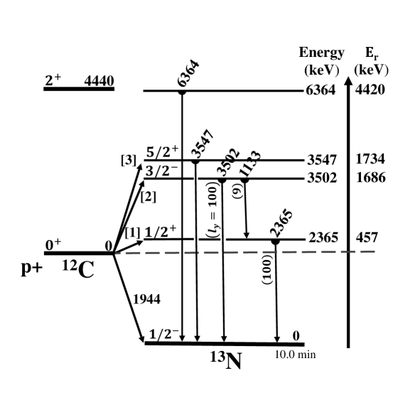
Figure 1: Level scheme of ¹³N (Not to scale)

The effective Lagrangian for the system can be written as [15, 16, 17]

$$\mathcal{L} =\psi_{p}^{{\dagger}}\left(iD_{t}+\frac{\vec{D}^{2}}{2m_{p}}\right)\psi_{p}+\psi_{c}^{{\dagger}}\left(iD_{t}+\frac{\vec{D}^{2}}{2m_{c}}\right)\psi_{c}$$ (1)

$$+\sum_{x}d_{x}^{{\dagger}}\left[\Delta_{x}+\sum^{N_{x}}_{n=1}\nu_{n,x}\left(iD_{t}+\frac{\vec{D}^{2}}{2m_{tot}}\right)^{n}\right]d_{x}$$

$$-\,\sum_{x}g_{x}\left[\,d_{x}^{{\dagger}}\left[\psi_{p}\,i\,\overleftrightarrow{\nabla}\,\psi_{c}\,\right]_{x}+\mathrm{h.c.}\right]+\cdots,$$

where $\psi_{p}$, $\psi_{c}$ and $d_{x}$ are the proton, ¹²C and the dicluster field, respectively, with the subscript $d_{x}$ denoting the total angular momentum and parity of the dicluster, $x=J^{\pi}$. Their masses are denoted as $m_{p}$, $m_{c}$ and $m_{tot}=m_{p}+m_{c}$, respectively, and the covariant derivatives are defined as $D_{\mu}=\partial_{\mu}+ie\hat{Q}A_{\mu}$, where $\hat{Q}$ is the charge operator. The parameters $\Delta_{x}$ and $g_{x}$ represent the residual masses and coupling constants of field $d_{x}$, respectively. The index $n$ is 1 for $s$- and $p$- waves, and runs up to 2 for $d$- wave. The $\nu_{1,x}$ in the kinetic term of the dicluster field are chosen as $\pm 1$ to be a sign related to the effective range [7], while the $\nu_{2,x}$ in the 2nd-order kinetic term for $d$-wave is needed for renormalization. At LO, we have therefore two low-energy constants (LECs) for $s$- and $p$-waves, and three low-energy constants for $d$-wave. As we will show shortly, these LECs are to be related to the effective range parameters.

The projection of the operator $\psi_{p}\,i\overleftrightarrow{\nabla}\psi_{c}=\psi_{p}\left(m_{c}i\reflectbox{$\vec{\reflectbox{$\nabla$}}$}-m_{p}i\vec{\nabla}\right)\psi_{c}/(m_{p}+m_{c})$ to the $x=1/2^{+},\,3/2^{-},\,1/2^{-}$, and $5/2^{+}$ states are given as [18]

$$\left[\psi_{p}i\overleftrightarrow{\nabla}\psi_{c}\right]_{\frac{1}{2}^{+}}^{m} =\sum_{m_{s}}C_{00,\frac{1}{2}m_{s}}^{\frac{1}{2}m}\,\psi_{p}\psi_{c},$$

$$\left[\psi_{p}i\overleftrightarrow{\nabla}\psi_{c}\right]_{\frac{3}{2}^{-}\left(\frac{1}{2}^{-}\right)}^{m} =\sum_{\alpha,m_{s}}C_{1\alpha,\frac{1}{2}m_{s}}^{\frac{3}{2}m\left(\frac{1}{2}m\right)}\,\psi_{p}i\overleftrightarrow{\nabla}_{\alpha}\psi_{c},$$

$$\left[\psi_{p}i\overleftrightarrow{\nabla}\psi_{c}\right]_{\frac{5}{2}^{+}}^{m} =\sum_{\alpha,\beta,m_{l},m_{s}}C_{2m_{l},\frac{1}{2}m_{s}}^{\frac{5}{2}m}C_{1\alpha,1\beta}^{2m_{l}}\psi_{p}$$ (2)

$$\times\ \frac{1}{2}\left(i\overleftrightarrow{\nabla}_{\alpha}i\overleftrightarrow{\nabla}_{\beta}+i\overleftrightarrow{\nabla}_{\beta}i\overleftrightarrow{\nabla}_{\alpha}\right)\psi_{c},$$

where $m_{s}$ is the spin projection of the proton and $C_{j_{1}m_{1},j_{2}m_{2}}^{Jm}$ is a short notation for the Clebsch-Gordan coefficients $\langle j_{1}m_{1},j_{2}m_{2}|(j_{1}j_{2})jm\rangle$. Here and hereafter, we use the Greek letters to denote spherical components that run from $-1$ to $1$. The conversion to Cartesian coordinates for convenience in the calculation of the $d$-wave can be found in Ref. [16].

II.2 The irreducible self-energy and renormalization conditions

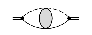
Figure 2: Self-energy diagram of a dicluster. The solid line denotes the core(¹²C) and the dashed line represents the proton field. The shaded bubble denotes the Coulomb Green’s function.

The full dicluster propagator of the dicluster $d_{x}$ reads

$$iD_{x}(E)=\frac{i}{\Delta_{x}+\sum_{n=1}^{N_{x}}\nu_{n,x}(E+i\epsilon)^{n}-\Sigma_{x}(E)},$$ (3)

where $\Sigma_{x}(E)$ is the irreducible self-energy shown in Fig. 2. The Coulomb interaction plays a crucial role at low-energy, and is taken into account by the Coulomb Green’s function. Because each dicluster of $x$ in our consideration has a different orbital angular momentum $l$, we will use $l$ and $x$ interchangeably hereafter.

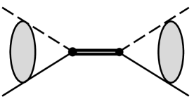
Figure 3: Scattering amplitude for elastic p-¹²C scattering. The notation is the same as in Fig. 2

The elastic scattering amplitude $T_{l}$ for $s$-, $p$- and $d$-waves are depicted in Fig. 3, and can be evaluated as [19]

$$T_{l}=g_{l}^{2}D_{l}(E)e^{2i\sigma_{l}}k^{2l}\hat{C}_{l}^{2}(\eta),$$ (4)

where $\sigma_{l}=\mathrm{arg}\Gamma(l+1+i\eta)$, and

$$\hat{C}_{l}(\eta)=\left|\Gamma(l+1+i\eta)\right|{\mathrm{e}}^{-\frac{1}{2}\pi\eta}/\Gamma(l+1),$$ (5)

which is the Gamow-Sommerfeld factor $C_{l}(\eta)$ [20, 9] but normalized to unity when $\eta$ goes to zero.

The scattering amplitude in Eq.(4) can be matched with the effective range function as [11]

$$T_{l}(E)=-\frac{2\pi}{m_{\mathrm{R}}}\frac{k^{2l}e^{2i\sigma_{l}}\hat{C}_{l}^{2}(\eta)}{f_{l}(k)-2k_{\mathrm{C}}h_{l}(\eta)}.$$ (6)

Here, $f_{l}(k)$ is the Coulomb-modified effective range function (ERF) [21, 22],

$$f_{l}(k) \equiv k^{2l+1}\hat{C}_{l}(\eta)^{2}\left(\mathrm{cot}\delta_{l}(k)-i\right)+2k_{\mathrm{C}}h_{l}(\eta)$$

$$= -\frac{1}{a_{l}}+\frac{1}{2}r_{l}k^{2}-\frac{1}{4}P_{l}k^{4}+\cdots,$$

where $\delta_{l}$ is the phase shifts relative to the regular Coulomb function for angular momentum $l$, $a_{l}$, $r_{l}$ and $P_{l}$ are the effective range parameters (scattering length, effective range and shape parameter), and the function $h_{l}(\eta)$ is defined as [23]

$$h_{l}(\eta)=k^{2l}\frac{\hat{C}_{l}(\eta)^{2}}{\hat{C}_{0}(\eta)^{2}}\left(\psi(i\eta)+\frac{1}{2i\eta}-\mathrm{log}(i\eta)\right),$$ (8)

where $\psi(z)=\Gamma^{\prime}(z)/\Gamma(z)$ is the logarithmic derivative of the Gamma function. Comparison of Eq.(6) with Eq.(4) enables us to renormalize the LECs in terms of the effective range parameters.

II.2.1 $S$-wave interaction

The irreducible self-energy of $s$-wave dicluster can be expressed as

$$\Sigma_{0}(E) = g_{0}^{2}\int\frac{d^{3}{\bm{k}}d^{3}{\bm{k}}^{\prime}}{(2\pi)^{6}}\left\langle{\bm{k}}|G_{\mathrm{C}}(E)|{{\bm{k}}^{\prime}}\right\rangle$$ (9)

$$= g_{0}^{2}\int\frac{d^{3}{\bm{p}}}{(2\pi)^{3}}\frac{\psi_{{\bm{p}}}(0)\psi_{{\bm{p}}}^{*}(0)}{E-{p^{2}}/2m_{\mathrm{R}}+i\epsilon},$$

where $G_{\mathrm{C}}(E)$ is the Coulomb Green’s function [24],

$$\left\langle{\bf r}|G_{\mathrm{C}}(E)|{\bf r^{\prime}}\right\rangle=\int\frac{d^{3}{\bm{p}}}{(2\pi)^{3}}\,\frac{\psi_{{\bm{p}}}({\bf r})\psi_{{\bm{p}}}^{*}({\bf r^{\prime}})}{E-\frac{{{\bm{p}}}^{2}}{2m_{\mathrm{R}}}+i\epsilon},$$ (10)

and $\psi_{{\bm{p}}}({\bf r})$ is the Coulomb wave function

$$\psi_{{\bm{p}}}({\bf r})=\sum_{l=0}^{\infty}(2l+1)i^{l}e^{i\sigma_{l}}\frac{F_{l}(\eta,pr)}{pr}P_{l}(\hat{p}\cdot\hat{r}),$$ (11)

$\eta=k_{\mathrm{C}}/p$, $F_{l}$ are the regular Coulomb functions  [25].

The integral in Eq.(9) can be evaluated by using the power divergence subtraction (PDS) method [24, 26, 27],

$$\Sigma_{0}(E) = -g_{0}^{2}\frac{k_{C}m_{\mathrm{R}}}{\pi}h_{0}(\eta)+\Sigma_{0}^{\mathrm{div}},$$ (12)

and the divergent part $\Sigma_{0}^{\mathrm{div}}$ is energy-independent, whose explicit form can be found in Refs. [26, 27].

The $s$-wave ERF with $l=0$ is then given as

$$f_{0}(k)=-\frac{2\pi}{g_{0}^{2}m_{\mathrm{R}}}(\Delta_{0}+\Sigma_{0}^{\mathrm{div}})-\frac{\pi\nu_{0}}{g_{0}^{2}m_{\mathrm{R}}^{2}}k^{2}.$$ (13)

Comparison of Eq.(13) with Eq.(6) gives us the renormalization conditions

$$\frac{1}{a_{0}} =\frac{2\pi}{g_{0}^{2}m_{\mathrm{R}}}\left(\Delta_{0}+\Sigma^{\mathrm{div}}\right),$$

$$r_{0} =-\frac{2\pi\nu_{0}}{g_{0}^{2}m_{\mathrm{R}}^{2}}.$$ (14)

II.2.2 $P$-wave interaction

By using a similar procedure as for the s-wave, the irreducible self-energy of $p$-wave dicluster can be derived as [7],

$$\Sigma_{1}(E) = \frac{1}{3}g_{1}^{2}\int\frac{d^{3}{\bm{p}}}{(2\pi)^{3}}\frac{p^{2}\hat{C}_{1}(\eta_{p})^{2}}{E-\frac{p^{2}}{2m_{\mathrm{R}}}+i\epsilon}$$ (15)

$$= g_{1}^{2}\frac{m_{\mathrm{R}}}{3\pi^{2}}\Big{[}-L_{3}-(k^{2}+k_{\mathrm{C}}^{2})L_{1}$$

$$+k^{2}(k^{2}+k_{\mathrm{C}}^{2})\int dp\frac{\hat{C}_{0}(\eta)^{2}}{k^{2}-p^{2}+i\epsilon}\Big{]}$$

$$= \frac{g_{1}^{2}m_{\mathrm{R}}}{6\pi}\left[-\frac{2}{\pi}L_{3}-\frac{2}{\pi}(k^{2}+k^{2}_{\mathrm{C}})L_{1}-2k_{\mathrm{C}}h_{1}(\eta)\right],$$

where

$$L_{n} =\int dp\,\hat{C}_{0}(\eta_{p})^{2}p^{n-1}.$$ (16)

It is then a simple task to show that the resulting $p$-wave ERF reads $f_{1}(k)=-\frac{1}{a_{1}}+\frac{1}{2}r_{1}k^{2}$ with

$$\frac{1}{a_{1}} =-\frac{6\pi}{m_{\mathrm{R}}}\left(\frac{\Delta_{1}}{g_{1}^{2}}-\frac{m_{\mathrm{R}}}{3\pi^{2}}L_{3}\right.\left.-\frac{m_{\mathrm{R}}}{3\pi^{2}}k_{\mathrm{C}}^{2}L_{1}\right),$$

$$r_{1} =\frac{6\pi\nu_{1}}{g_{1}^{2}m_{\mathrm{R}}^{2}}-\frac{4}{\pi}L_{1}.$$ (17)

II.2.3 $D$-wave interaction

By adopting the trick of using Cartesian representation of the $d$-wave vertex function [17, 28], the irreducible self-energy of $d$-wave dicluster can be evaluated as

$$\Sigma_{2}(E) = g_{2}^{2}\frac{2}{15}\int\frac{d^{3}p}{(2\pi)^{3}}\frac{p^{4}\hat{C}_{2}(\eta_{p})^{2}}{E-\frac{p^{2}}{2m_{\mathrm{R}}}+i\epsilon}$$ (18)

$$= \frac{g_{2}^{2}m_{\mathrm{R}}}{15\pi}\left[\left(-\frac{8}{\pi}L_{5}-\frac{10}{\pi}k_{\mathrm{C}}^{2}L_{3}-\frac{2}{\pi}k_{\mathrm{C}}^{4}L_{1}\right)\right.$$

$$\left.+\left(-\frac{8}{\pi}L_{3}-\frac{10}{\pi}k_{\mathrm{C}}^{2}L_{1}\right)k^{2}-\frac{8}{\pi}L_{1}k^{4}-2k_{\mathrm{C}}h_{2}(\eta)\right].$$

The corresponding $d$-wave ERF is then given as $f_{2}(k)=-\frac{1}{a_{2}}+\frac{1}{2}r_{2}k^{2}-\frac{1}{4}P_{2}k^{4}$ with

$$\frac{1}{a_{2}} =\frac{15\pi}{g_{2}^{2}m_{\mathrm{R}}}\Delta_{2}+\frac{8}{\pi}L_{5}+\frac{10}{\pi}k_{\mathrm{C}}^{2}L_{3}+\frac{2}{\pi}k_{\mathrm{C}}^{4}L_{1},$$

$$r_{2} =-\frac{15\pi\nu_{1,2}}{g_{2}^{2}m_{\mathrm{R}}^{2}}-\frac{16}{\pi}L_{3}-\frac{20}{\pi}k_{\mathrm{C}}^{2}L_{1},$$

$$P_{2} =\frac{15\pi\nu_{2,2}}{m_{\mathrm{R}}^{3}g_{2}^{2}}+\frac{32}{\pi}L_{1}.$$ (19)

III Numerical results and discussion

III.1 Fitting to experimental data

In the previous section, we have shown that the cluster EFT description with the LECs is identical to the Coulomb-modified ERF with a finite number of effective range parameters (ERPs), and the remaining task is to determine the values of the parameters from the experimental data.

We find that the fitting for the ERPs is complicated due to the strong correlations between the ERPs of the $p$ and $d$-waves, which is caused mainly by the fact that their pole positions are very close to each other. This problem can be avoided by rewriting the effective range function as a series around the pole position,

$$f_{l}(k) =-\frac{1}{a_{l}}+\frac{1}{2}r_{l}k^{2}-\frac{1}{4}P_{l}k^{4}+Q_{l}k^{6}+\cdots$$ (20)

$$=\frac{1}{2}r_{l}^{{}^{\prime}}(k^{2}-k_{r}^{2})-\frac{1}{4}P_{l}^{{}^{\prime}}(k^{2}-k_{r}^{2})^{2}$$

$$\,\,\,\,+\,Q_{l}^{{}^{\prime}}(k^{2}-k_{r}^{2})^{3}+\cdots,$$

where $k_{r}^{2}\equiv m_{\mathrm{R}}E_{r}$, $E_{r}$ being the resonance excitation energy, and $(E_{r},r_{l}^{{}^{\prime}},P_{l}^{{}^{\prime}},Q_{l}^{{}^{\prime}},\cdots)$ are another representation of the ERPs $(a_{l},r_{l},P_{l},Q_{l},\cdots)$.

The parameters $(E_{r}^{{}^{\prime}}=E_{r},\,r_{l}^{{}^{\prime}},\,P_{l}^{{}^{\prime}},\,Q_{l}^{{}^{\prime}},\,\cdots)$ are determined by minimizing $\chi_{\Lambda}^{2}$ defined as

$$\chi_{\Lambda}^{2}=\sum_{i}^{N}\frac{\left|y_{i,\text{th}}-y_{i,\text{exp}}\right|^{2}}{\Delta y_{i,\text{exp}}^{2}+\Delta y_{i,\text{th}}^{2}}$$ (21)

where $y_{i,\text{exp}}$ ($y_{i,\text{th}}$) is the experimental (theoretical) differential cross sections at a given angle, $\Delta y_{i,\text{exp}}$ are error bars of the data. Some of the data have very small $\Delta y_{i,exp}$, and the usual chi-square is dominated by them. As a regulator that takes into account the theoretical uncertainty, we introduce

$$\Delta y_{i,\text{th}}\equiv y_{i,\text{exp}}\times\frac{k_{i}}{\Lambda},$$ (22)

where $\Lambda$ is a parameter. While constructed in an ad-hoc manner, this form is motivated by the fact that the EFT description is less accurate at high momentum. $\Delta y_{i,\text{th}}$ should not be bigger than the uncertainty of the theory, and thus we choose $\Lambda=1$ GeV. We find that the resulting parameters are found to be stable and insensitive to the values of $\Lambda$, while the value of $\chi_{\Lambda}^{2}$ increases with $\Lambda$.

So far, we have considered only the leading order (LO) terms, and the resulting theory turns out to be identical to the Coulomb-modified effective range expansion with the parameters $(E_{r},r_{l}^{{}^{\prime}})$ for $s$- and $p$-waves and $(E_{r},r_{l}^{{}^{\prime}},P_{l}^{{}^{\prime}})$ for $d$-wave. While we do not describe explicitly here, going to the next order (or NLO) with including one higher-order terms in the Lagrangian is also identical to the effective range expansion with one more term, that is, $(E_{r},r_{l}^{{}^{\prime}},P_{l}^{{}^{\prime}})$ for $s$- and $p$-waves and $(E_{r},r_{l}^{{}^{\prime}},P_{l}^{{}^{\prime}},Q_{l}^{{}^{\prime}})$ for $d$-wave, which we denote as NLO. We also consider the leading order calculation where the $J^{\pi}=\frac{1}{2}^{-}$ ground state of ¹³N is also taken as a pertinent degrees of freedom, which we denote as LO+gs. We thus have three sets of parameters, LO, NLO and LO+gs.

The parameters of each set are then determined by the fitting to the differential cross-section data at three different angles, 89.1, 118.7, and 146.9 degrees [29]. Figures 4 and  5 show the resulting differential cross-sections for the region $E_{p}\leq 0.7\ \text{MeV}$ and $E_{p}=(0.7\sim 2)\ \text{MeV}$, $E_{p}$ is the incident proton energy. The calculated cross sections agree very well with the data, which can also be seen in the obtained $\chi_{\Lambda}^{2}/\text{datum}=1.20$ for LO, and 1.03 for NLO.

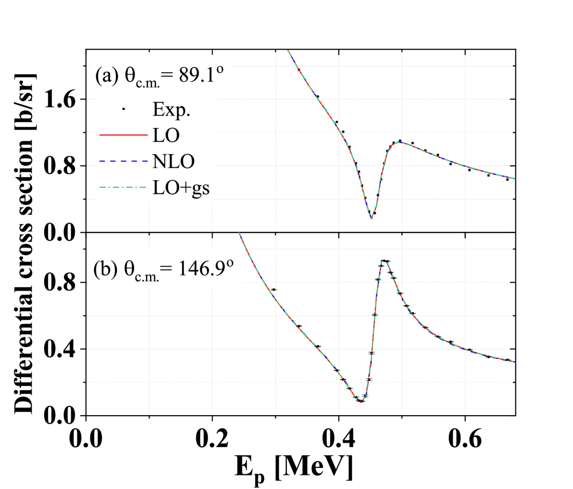
Figure 4: The differential cross section for elastic p-¹²C scattering as a function of the proton energy $E_{p}<0.7$ MeV at two angles (a) 89.1^∘ and (b) 146.9^∘. The red, blue, and green solid lines represent the EFT results at LO, NLO, and LO+gs. The black circles represent the experimental data  [29].

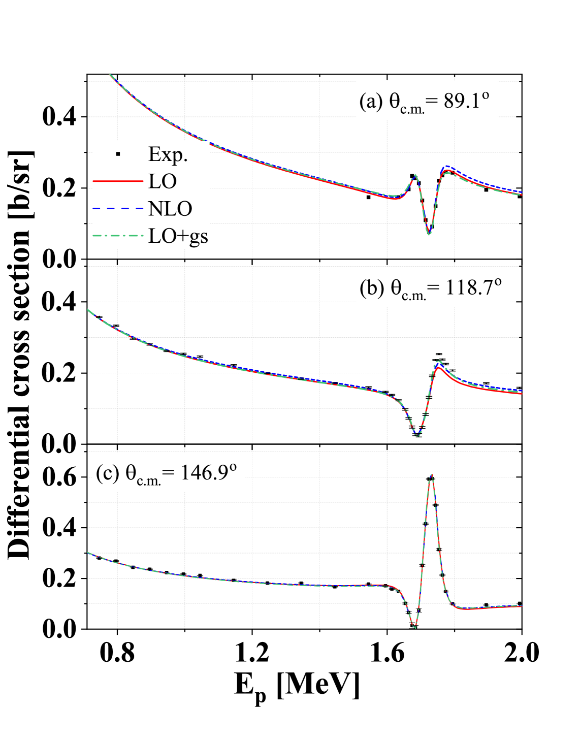
Figure 5: The differential cross section for elastic p-¹²C scattering as a function of the proton energy $E_{p}=(0.7\sim 2)$ MeV at three angles (a) 89.1^∘, (b) 118.7^∘ and (c) 146.9^∘. The notation is the same as in Fig. 4.

The values of the fitted ERE parameters for the expansion around the origin are summarized in Table 1. In the NLO case, compared to LO, the added parameters, the $P_{1}^{\prime}$ for the $p_{3/2}$-wave and the $P_{2}^{\prime}$ and $Q_{2}^{\prime}$ for the $d_{5/2}$-wave, have large uncertainties that are much bigger than the central values. This might be due to a strong correlation between the parameters of $p_{3/2}$ and $d_{5/2}$-waves, which is not surprising since the pole positions at 1.686 and 1.734 MeV, respectively, are very close to each other.

We also considered the role of the ground state on the differential cross-sections. Our results show that including the ground state provides a more accurate description of differential cross-section in high energy region, particularly around 1.7 MeV. Our result is in line with the finding obtained from the $R$-matrix study given in Ref. [6]. Fig. 6 shows that the ground state gives us a small and slowly varying repulsive contribution. As can be seen in Table 1, the pole position parameter for this channel suffers from a very big uncertainty, $E_{r}=(-1\pm 13)$ MeV, which is not surprising recalling that the ground state lies below about 1.9 MeV from the threshold.

Table 1: The ERE parameters for the expansion around the pole positions.

	$E_{r}$ (MeV)	$r_{l}^{{}^{\prime}}$ (fm1-2l)	$P_{l}^{{}^{\prime}}$ (fm3-2l)	$Q_{l}^{{}^{\prime}}$ (fm5-2l)
(a) LO $\chi_{\Lambda}^{2}/N=1.20$
$s_{1/2}$	$-0.09\pm 0.00$	$1.52\pm 0.00$
$p_{3/2}$	$1.74\pm 0.00$	$-1.83\pm 0.04$
$d_{5/2}$	$1.76\pm 0.01$	$-0.19\pm 0.02$	$4.94\pm 2.65$
(b) NLO $\chi_{\Lambda}^{2}/N=1.03$
$s_{1/2}$	$-0.11\pm 0.00$	$1.46\pm 0.01$	$-2.18\pm 0.11$
$p_{3/2}$	$1.74\pm 0.02$	$-2.01\pm 0.42$	$25.40\pm 55.15$
$d_{5/2}$	$1.78\pm 0.02$	$-0.16\pm 0.03$	$0.12\pm 3.83$	$(3.35\pm 6.69)\times 10^{-6}$
(c) LO+gs $\chi_{\Lambda}^{2}/N=1.01$
$s_{1/2}$	$-0.09\pm 0.00$	$1.52\pm 0.00$
$p_{3/2}$	$1.74\pm 0.00$	$-1.91\pm 0.04$
$d_{5/2}$	$1.77\pm 0.01$	$-0.18\pm 0.02$	$2.14\pm 2.86$
$p_{1/2}$	$-1.02\pm 12.98$	$-0.20\pm 0.98$

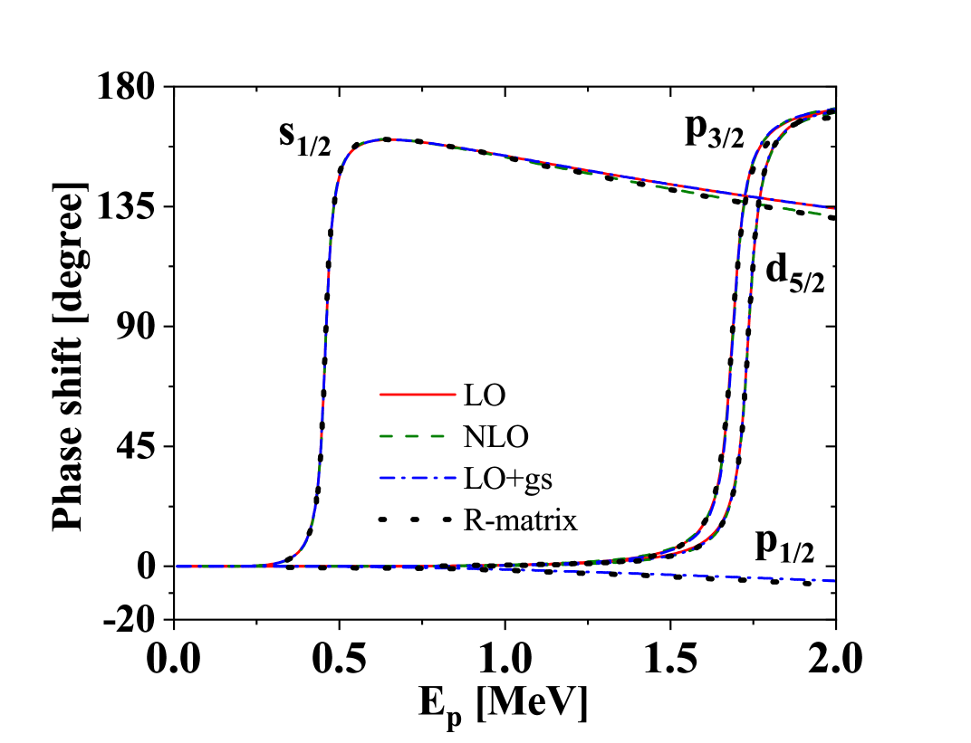
Figure 6: The phase shifts. The red, green and blue lines are for LO, NLO and LO+gs, respectively. The black short-dashed lines are the results by using the $R$-matrix taken from Ref. [6].

The phase shifts are plotted and compared with the $R$-matrix analysis in Fig. 6. As can be seen in Fig. 6, our results are very close to those obtained by $R$-matrix calculations [6].

IV Conclusions

The elastic p-¹²C scattering at energies below $E_{p}\leq 2\ \text{MeV}$ is studied in terms of a cluster EFT, the pertinent degrees of freedom of which are the proton, the ground state of ¹²C and the three low-lying states ($s_{1/2}$, $p_{3/2}$, $d_{5/2}$) of ¹³N. The resulting scattering amplitudes of the theory are found to be consistent with the Coulomb-modified ERE, and the low-energy constants are represented by the ERE parameters. At the leading-order, we have seven parameters, 2 for each of the $s$- and $p$-wave, and 3 for the $d$-wave. The theory prediction turns out to be in a very good agreement with the experimental data, achieving $\chi_{\Lambda}^{2}/\text{datum}=1.20$ (see Eqs. (21,22) for the definition of $\chi_{\Lambda}^{2}$).

The fitting procedure for the ERE parameters can be substantially simplified by expanding the ERE around the pole positions and defining the ERE parameters accordingly, which strongly reduces correlations among the parameters. The effect of the higher-order terms has been studied by adding one higher-order term for each partial wave, which is denoted as NLO and scores $\chi_{\Lambda}^{2}/\text{datum}=1.03$. To estimate the role of the ground state of ¹³N that lies below the threshold, we have also considered the cases where the ground state is promoted to an explicit degree of freedom. The resulting “LO+gs” theory results in $\chi_{\Lambda}^{2}/\text{datum}=1.01$. These improvements of NLO and LO+gs are, however, accompanied by large uncertainties in the additionally introduced ERE parameters (see Table 1). It shows that the experimental data considered in this work with $E_{p}\leq 2$ MeV are well described by the LO, and the contributions from the higher order terms and the sub-threshold ground state are not essential. The resulting phase shifts are in an excellent agreement with the $R$-matrix analysis [6].

The high momentum scale of a low-energy EFT is set by the lowest-energy state that is not taken explicitly, the $2^{+}$ state of ¹²C with $E_{x}=4.44\ \text{MeV}$. This corresponds to rather a large expansion parameter $k_{lo}/k_{hi}\,=\,(0.3\sim 0.6)$. The main mechanism that makes our approach successful despite this rather large ratio might be traced to the relevance of the ERE at low energies. An immediate extension of this work would be ${}^{12}\mathrm{C}(p,\gamma)^{13}\mathrm{N}$.

References

- Agostini et al. [2020] M. Agostini et al. (BOREXINO), Nature 587, 577 (2020), arXiv:2006.15115 [hep-ex] .
- Mowlavi et al. [1998] N. Mowlavi, A. Jorissen, and M. Arnould, Astronomy and Astrophysics 334, 153 (1998).
- Kabir et al. [2020] A. Kabir, B. Irgaziev, and J.-U. Nabi, Brazilian Journal of Physics 50, 112 (2020).
- Huang et al. [2010] J. Huang, C. Bertulani, and V. Guimaraes, Atomic Data and Nuclear Data Tables 96, 824 (2010).
- Li et al. [2010] Z. Li, J. Su, B. Guo, Z. Li, X. Bai, J. Liu, Y. Li, S. Yan, B. Wang, Y. Wang, et al., Science China Physics, Mechanics and Astronomy 53, 658 (2010).
- Azuma et al. [2010] R. E. Azuma, E. Uberseder, E. C. Simpson, C. R. Brune, H. Costantini, R. J. de Boer, J. Görres, M. Heil, P. J. LeBlanc, C. Ugalde, and M. Wiescher, Phys. Rev. C 81, 045805 (2010).
- Bertulani et al. [2002] C. Bertulani, H.-W. Hammer, and U. Van Kolck, Nuclear Physics A 712, 37 (2002).
- Acharya and Phillips [2013] B. Acharya and D. R. Phillips, Nuclear Physics A 913, 103 (2013).
- Ryberg et al. [2014a] E. Ryberg, C. Forssén, H.-W. Hammer, and L. Platter, Phys. Rev. C 89, 014325 (2014a).
- Zhang et al. [2015] X. Zhang, K. M. Nollett, and D. Phillips, Physics Letters B 751, 535 (2015).
- Higa et al. [2008] R. Higa, H.-W. Hammer, and U. Van Kolck, Nuclear Physics A 809, 171 (2008).
- Ando [2016] S.-I. Ando, The European Physical Journal A 52, 1 (2016).
- Ando [2018a] S.-I. Ando, Phys. Rev. C 97, 014604 (2018a).
- Hammer et al. [2020] H.-W. Hammer, S. König, and U. van Kolck, Rev. Mod. Phys. 92, 025004 (2020).
- Ryberg et al. [2014b] E. Ryberg, C. Forssén, H.-W. Hammer, and L. Platter, The European Physical Journal A 50, 1 (2014b).
- Bedaque et al. [2003] P. Bedaque, H.-W. Hammer, and U. Van Kolck, Physics Letters B 569, 159 (2003).
- Braun et al. [2019] J. Braun, W. Elkamhawy, R. Roth, and H. Hammer, Journal of Physics G: Nuclear and Particle Physics 46, 115101 (2019).
- Tanabashi et al. [2018] M. Tanabashi, K. Hagiwara, K. Hikasa, K. Nakamura, Y. Sumino, F. Takahashi, J. Tanaka, K. Agashe, G. Aielli, C. Amsler, et al., Physical Review D 98 (2018).
- Ando [2018b] S.-I. Ando, Physical Review C 97, 014604 (2018b).
- Abramowitz and Stegun [1984] M. Abramowitz and I. A. Stegun, Thun-Frankfurt/Main (1984).
- Berger and Spruch [1965] R. O. Berger and L. Spruch, Phys. Rev. 138, B1106 (1965).
- König [2013] S. König, Dissertation, Bonn (2013).
- Jackson and Blatt [1950] J. D. Jackson and J. M. Blatt, Reviews of Modern Physics 22, 77 (1950).
- Kong and Ravndal [2000] X. Kong and F. Ravndal, Nuclear Physics A 665, 137 (2000).
- König et al. [2013] S. König, D. Lee, and H. Hammer, Journal of Physics G: Nuclear and Particle Physics 40, 045106 (2013).
- Kong and Ravndal [1999] X. Kong and F. Ravndal, Physics Letters B 450, 320 (1999).
- Ando et al. [2007] S.-i. Ando, J. W. Shin, C. H. Hyun, and S.-W. Hong, Physical Review C 76, 064001 (2007).
- Brown and Hale [2014] L. S. Brown and G. M. Hale, Physical Review C 89, 014622 (2014).
- Meyer et al. [1976] H. Meyer, G. Plattner, and I. Sick, Zeitschrift für Physik A Atoms and Nuclei 279, 41 (1976).