Electroweak Transitions Involving Resonances

Abstract

The increasing importance of hadronic resonances in our understanding of the Standard Model is underscored by recent advancements in lattice Quantum Chromodynamics (QCD) calculations. We review recent developments, with a particular emphasis on electroweak transitions that result in two-hadron final states. Additionally, we present the finite-volume lattice QCD methodologies that are pivotal in such studies in the context of preliminary results from the $B\to\pi\pi\ell\bar{\nu}$.

1 Introduction

Electroweak transitions, mediated by the $W^{\pm}$ and $Z$ bosons and the photon $\gamma$, are fundamental in understanding particle behavior, especially in processes involving quark flavor or lepton number changes. These transitions have significantly advanced our comprehension of the Standard Model, shedding light on electroweak symmetry breaking and the origins of particle masses. Furthermore, they are pivotal in exploring CP violation, illuminating our understanding of the universe’s matter-antimatter asymmetry. Electroweak transitions also serve as a critical tool for probing the limits of the Standard Model and searching for new physics by investigating rare decays and anomalies that might indicate new particles or interactions.

Lattice QCD has been instrumental in determining the elements of the CKM matrix [1], a cornerstone achievement in the field. The collaborative efforts of the past 15 years, coupled with global experimental endeavors, have yielded precise determinations of key Standard Model parameters, for example $V_{ud}$, $V_{us}$, $V_{cd}$, $V_{cs}$, to a few percent accuracy. However, these efforts have predominantly focused on initial and final states comprising QCD-stable hadrons, neglecting hadronic resonances.

Hadronic resonances, a significant part of the hadron spectrum, are characterized by their brief lifetimes and rapid decay into other hadron states. In experiments, these resonances manifest as distinct enhancements in the energy-dependent cross-section of certain final states. A particularly interesting exemple is the rare decay of a $B$-meson, particularly the process $B\to K^{\star}(892)\ell\ell$, as depicted in Fig. 1.

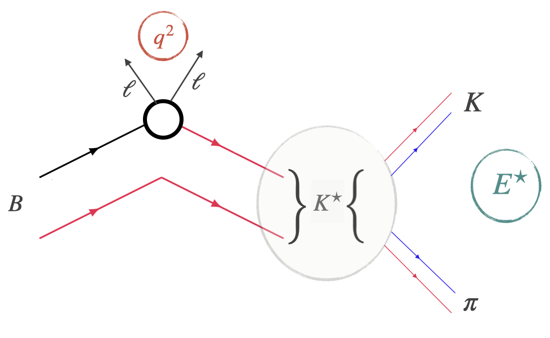
Figure 1: Illustrative representation of a rare $B$ decay, highlighting the transition of a $\bar{b}$-quark in the $B$-meson to a $s$-quark and a pair of leptons $\ell$, resulting in the formation of a $K^{\star}$ resonance which subsequently decays into a pion ($\pi$) and a kaon ($K$).

The decay of the initial $B$-meson through the electroweak interaction results in a $\bar{b}$-quark transforming into a $\bar{s}$-quark and a pair of leptons $\ell$ via a loop process, as indicated in Fig. 1. The momentum transfer, denoted as $q^{2}$, corresponds to the energy carried away by the two leptons. The newly formed $\bar{s}$-quark, in combination with the existing light $u$-quark from the $B$-meson, generates a hadron with an $\bar{s}$-quark and a light $u$-quark. Due to its nature, this process allows for the creation of hadronic states with angular momentum $J=0,1,\ldots$. Below the three-particle threshold, these states predominantly manifest as kaon ($K$) and pion ($\pi$) pairs at a specific two-hadron invariant mass, $E^{\star}$. The dynamic interplay of $K$ and $\pi$, which are stable against strong interaction decay, enters in their rescattering process, which can induce the formation of a $K^{\star}$ resonance, an unstable hadron state observed as a significant enhancement in the $E^{\star}$ dependence of the partial cross-section in $K\pi$ scattering [2].

While $K^{\star}$ resonances are often treated as stable hadrons for analytical simplicity, it is essential to recognize their highly transient nature, with lifespans of approximately $10^{-23}$ seconds before decaying through Quantum Chromodynamics (QCD) into a $K$ and $\pi$ pair [3]. Therefore, the relevant final states extend beyond the ephemeral $K^{\star}$ resonances to the QCD asymptotic states, particularly the $K$ and $\pi$. To effectively discuss Electroweak Transitions Involving Resonances, it is necessary to consider Electroweak Transitions leading to multihadron final states; more specifically two-hadron final states. This text is organized as follows: Sec.2 reviews the most significant processes in lattice QCD and experiment. Sec.3 provides an overview of the lattice QCD methodologies applied in these calculations, along with an example workflow. Sec. 4 discusses some promising topics for the near-term future, and Sec.5 offers a summary.

2 Current Status

We consider three types of electroweak processes involving multi-hadron final states: purely hadronic electroweak transitions, photoproduction of hadronic resonances, and semileptonic electroweak processes.

Purely Hadronic Electroweak Transitions

The primary focus within purely hadronic electroweak transitions is the $K\to\pi\pi$ process, critical for enhancing our understanding of CP violation and the pronounced matter-antimatter asymmetry, which diverges significantly from Standard Model predictions. In this process, an $s$-quark in the Kaon emits a $W$ boson, converting it into a $u$ quark. The $W$ boson, rather than decaying into a lepton-antineutrino pair, produces a pair of $u$ and $d$ quarks. These quarks subsequently form hadrons with the remaining light quarks, resulting in two pions in the final state. These pions can exist in two isospin states, $I=0$ and $I=2$, with the relevant partial waves being $\ell=0$ and $\ell=2$ due to Bose symmetry.

Three lattice QCD calculations of the $K\to\pi\pi$ process exist: two by the RBC/UKQCD collaboration [4, 5, 6] and one by Ishizuka et al. [7]. Both RBC/UKQCD calculations use Möbius Domain wall fermions at quark masses corresponding to the physical point; they, however, employ different lattice spacings: Ref. [4, 5] used $a=0.1433$ fm and Ref. [6] $a\approx 0.1932$ fm. The first calculation [4] and its improvement [5] made use of the twisted-G-parity boundary condition to maximize the signal, which is best when the two pions final state energy matches the initial state kaon energy. The second RBC/UKQCD calculation [6] made use of distillation [8] combined with periodic boundary conditions to construct the initial and final states. The crucial part of both calculations was a well-determined scattering phase shift for the $I=0,\ell=0$ $\pi\pi$ channel. The resulting $Re(\tfrac{\epsilon^{\prime}}{\epsilon})$ values are shown in Fig. 2, and the reader is directed to Ref. [6] for further details. The calculation by Ishizuka et al. [7] was performed with Clover fermions with quark masses corresponding to $m_{\pi}\approx 260$ MeV and a single lattice spacing of $0.091$ fm and found a ratio of $Re(\tfrac{\epsilon^{\prime}}{\epsilon})=1.9(5.7)\times 10^{-}3$; At the same time, their result is still statistically compatible with zero (and thus not shown in Fig. 2), further efforts are warranted to verify the $Re(\tfrac{\epsilon^{\prime}}{\epsilon})$ results from RBC/UKQCD.

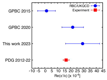
Figure 2: Figure taken from Ref. [6]; shown is the value for $Re(\tfrac{\epsilon^{\prime}}{\epsilon})$ from RBC/UKQCD calculations as well as the PDG value.

Experimentally, the $K\to\pi\pi$ processes were measured at the NA48 [9] and KTeV experiments [10]. They remain a primary source of background in ongoing experiments like KOTO [11, 12] and NA62 [13], necessitating a robust Standard Model understanding. Hence, precise lattice QCD determinations of these processes continue to play a crucial role in our comprehension of the Standard Model.

In the community’s effort to understand CP violation, Hansen et al. are pushing forward our understanding of CP violation in the charm sector with pioneering calculations of the $D\to\pi\pi$ process [14]. At the same time, there are plenty of other processes of interest; they are more challenging from both the formal and computational approaches.

Photoproduction of Hadronic Resonances

In the realm of photoproduction of hadronic resonances, lattice QCD calculations have been conducted for the $\pi\gamma\to\pi\pi$ and $K\gamma\to K\pi$ processes, while a toy model analysis discusses the coupled channel approach and preliminary results of the $\gamma\to\pi\pi|K\bar{K}$ demonstrate the feasibility of a coupled channel calculation. The $\pi\gamma\to\pi\pi$ process, besides serving as a testbed for lattice QCD methodologies, contributes to determining the dispersive determination of the $(g-2)\mu$ by ascertaining the chiral anomaly $F{3\pi}$, and $\gamma\to\pi\pi|K\bar{K}$ might offer insight into where the pure Yang-Mills glueballs have gone in the dynamic QCD spectrum.

The $\pi\gamma\to\pi\pi$ process is perhaps the simplest for testing the relevant lattice QCD methodologies. There, the photon excites the pion ($I(J^{P})=1(0^{-}))$, where the spins of the quarks are anti-parallel, to a $\rho$ $(I(J^{P})=1(1^{-}))$, where the spins are parallel. As the $\rho$ is a hadronic resonance, it decays to a pair of pions in $P$-wave with a branching fraction larger than $99.9$ % and a decay width of approximately $\Gamma=150$ MeV [3]. The first lattice QCD determination of the $\pi\gamma\to\pi\pi$ transition amplitude was performed by HadSpec [15], where they used Clover-Wilson fermions on an anisotropic lattice with quark masses corresponding to $m_{\pi}\approx 400$ MeV and a single lattice spacing, $a_{s}\approx 0.12$ fm. LHPC followed up the calculation [16] on isotropic lattices with Clover-Wilson fermions and a pion mass of $\approx 320$ MeV and a lattice spacing of approximately $0.114$ fm. The combined results were used in the determination of $F_{3\pi}$ in Ref. [17].

The $K\gamma\to K\pi$ process is very similar to the $\pi\gamma\to\pi\pi$, except an $s$-quark replaces a light quark. HadSpec conducted the sole calculation for this process. So far, the only calculation of this process was determined by HadSpec [18], where they used Clover-Wilson fermions on a single gauge ensemble with a lattice spacing $a_{s}\approx 0.12$ fm and a light quark mass corresponding to $m_{\pi}\approx 280$ MeV.

The $\gamma\to\pi\pi|K\bar{K}$ process produces states out of the vacuum; in this case, it creates a pair of pions or a pair of kaons. The two pions can resonate and produce a $\rho$ resonance, while the $K\bar{K}$ seems mostly decoupled [19]. The time-like pion form factor can be determined from the transition amplitude, which plays an important role in the $(g-2)_{\mu}$ [20]; the process also offers insights into the quark content of hadronic resonances and has implications for the understanding of glueballs outside pure Yang-Mills theory [21].

Experimentally, the photoproduction (or the reverse, radiative decay) processes are measured at the GlueX [22] experiment at JLab and (hopefully one day) also at PANDA at GSI [23].

Semileptonic Electroweak Processes

Although no published works currently exist on semileptonic electroweak processes involving resonances with a complete finite-volume treatment, preliminary results on the $B\to\pi\pi\ell\bar{\nu}$ process are discussed in Sec. 3. In this process, the $b$-quark in the $B$-meson emits a $W$ boson, which then further decays into a pair of $\ell\bar{\nu}$, while the $b$-quark changes to a $u$-quark. This transition offers a new probe for the smallest and least known of the CKM matrix elements, $V_{ub}$; the current value predominantly comes from the $B\to\pi\ell\bar{\nu}$ process, as can be seen in Fig. 3.

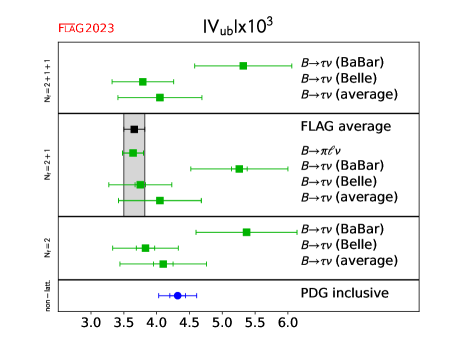
Figure 3: Figure taken from Ref. [1]; shown are the $V_{ub}$ matrix elements as determined from different experiments and different processes; both inclusive and exclusive analyses are shown. The average value its uncertainty for $V_{ub}=3.64(16)$ [1] are dominated by the semileptonic decay, $B\to\pi\ell\bar{\nu}$.

Due to the large variation in the $V_{ub}$ determinations, and in particular due to the fairly large difference ($\approx 1.7\sigma$ when all uncertainties are included [1]) between the inclusive and exclusive determination, an additional, new exclusive process to determine $V_{ub}$ is needed to understand the source of the tension better. The process $B\to\pi\pi(\to\rho)\ell\bar{\nu}$, actively measured at Belle II [24] and Belle [25], serves as a crucial alternative for determining $V_{ub}$, helping resolve tensions between inclusive and exclusive determinations. Furthermore, as it has more form factors than the $B\to\pi\ell\bar{\nu}$ process, it is also better for searching for potential Beyond the Standard Model contributions.

Semileptonic decays extend beyond mesons to baryons, particularly in the radiative and electroweak productions of the $\Delta(1232)$ resonance on a nucleon, a process vital for the success of the DUNE experiment [26, 27, 28].

3 Lattice Technology

In lattice QCD, the determination of infinite-volume transition amplitudes, as depicted in Fig. 4, involves a comprehensive workflow encompassing both spectrum and matrix element analysis: the top half of the diagram schematically shows the spectrum analysis, while the bottom half shows the matrix element analysis.

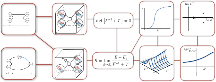
Figure 4: Schematic representation of the process to determine infinite-volume scattering and transition amplitudes from lattice QCD data. The top half illustrates the spectrum analysis workflow, while the bottom details the matrix element analysis.

The spectrum analysis, now a routine computation in many groups, starts with defining the energy region of interest. For the $\rho$ resonance, it is sufficient to go approximately to the $K\bar{K}$ threshold. We pick a set of interpolating operators $\mathcal{O}_{a}$ of the necessary types - for the $\rho$ on our ensemble with $m_{\pi}\approx 320$ MeV and $a\approx 0.114$ fm, two types suffice: $\bar{q}q(P)$ and $\pi(p_{1})\pi(p_{2})$, where $P$ is the size of the total momentum of the system and $p_{1}$ and $p_{2}$ are the sizes of the momenta belonging to the two pions. They are connected to $P$ through $\vec{P}=\vec{p}_{1}+\vec{p}_{2}$. From these interpolating operators, we construct a correlation matrix $C_{ab}(t)=\langle 0|\mathcal{O}_{a}(t)\mathcal{O}^{\dagger}_{b}(0)|0\rangle$, which we proceed to calculate through Wick contractions and whichever technology we prefer to employ for the propagators - this is represented by the left-most diagram on the top half of Fig. 4. In the preliminary results presented below, we employ a combination of forward, sequential, and stochastic propagators [29]. However, distillation is a great alternative when complicated sources are needed [8].

The correlation matrix $C_{ab}(t)$ contains information on the spectrum $E_{n}$ and the overlap between the states, $n$, in the energy region and the interpolating operators, $a$, $Z_{a}^{n}$:

$$C_{ab}(t)=\sum_{n}\frac{Z_{a}^{n}Z_{b}^{n,*}}{2E_{n}}e^{-E_{n}t}.$$ (1)

To extract the overlaps and the spectrum from the correlation matrix, we solve the variational problem:

$$C_{ab}(t)u_{b}^{n}(t)=\lambda_{n}(t,t_{0})C_{ab}(t_{0})u_{b}^{n}(t),$$ (2)

$$u_{a}^{n}(t)C_{ab}(t)u_{b}^{m}(t)=\delta^{nm},$$ (3)

Where $u$’s are the generalized eigenvectors and play an important role also in the matrix element analysis; $\lambda_{n}(t,t_{0})$ are principal correlators, which can be fit with a one, two, or more state models to determine the spectrum $E_{n}$. We can repeat this analysis on multiple volumes and in multiple irreducible representations. For the presented data, we employ a single volume, $32^{3}\times 96$, with a lattice spacing of $a=0.114$ fm and all irreducible representations that have a $J^{P}=1^{-}$ state in them for total momenta $P<\frac{2\pi}{L}\sqrt{3}$ [29].

The spectrum, i.e., the set of energies $E_{n}$, can be related to the infinite-volume scattering amplitude $T$ in what is often referred to as the Lüscher analysis, as depicted in the second-to-left and middle top diagram of Fig. 4. The Quantization Condition was first derived by Lüscher [30] in the context of relativistic quantum mechanics:

$$\det\left[F^{-1}(E)+T(E)\right]\bigg{|}_{E=E_{n}}=0,$$ (4)

followed up by Ref. [31] with a Quantum Field Theory derivation, where in a very simplistic view, the finite-volume two-point correlation function as a function energy $E$, instead of time $t$ as in Eq. 1, is expanded as a sum over poles; each pole belongs to a particular energy level. Its position is on the real axis and depends on the lattice parameters, $L$ and quark masses, and the scattering amplitude $T$. Further information about the Lüscher analysis can be found in Refs. [32, 33, 34, 35, 36].

At this point of the analysis, there are already two parts that involve fitting data to mathematical models, which can, in principle, introduce changes in the data - to quantify this uncertainty, we vary the mathematical models we fit, both for the principal correlators as well as the scattering amplitude and assign a systematic uncertainty to the parameters.

The resulting scattering amplitude can then be used to calculate the cross-section, although not very useful, as we have yet to learn how to make an experiment that will scatter two pions. We can, however, calculate the phase shift $\delta$ - first-from-middle diagram of Fig. 4, which is related to the scattering amplitude $T\propto\frac{1}{\cot{\delta}-i}$. If we are looking for hadronic resonances (and bound/virtual bound states included), we search for poles of the scattering amplitude $T$ in all the relevant Riemann sheets.

The matrix element analysis is similar in spirit - except that now we have a new process in mind. The $B\to\pi\pi\ell\bar{\nu}$, has a $B$-meson at the source, which propagates forward until the $b$-quark transitions to a $u$-quark through an emission of a $W$ boson; the transition is taken into account as an external local current insertion, $J_{EW}=\bar{u}(\gamma_{\mu}-\gamma_{5}\gamma_{\mu})b$. One option after the current is that the light quark from the current connects with the light quark from the $B$-meson, and another option is that a pair of light quark-antiquarks are made up from the vacuum, and the light quark connects with one of them. The latter is described by an interpolating operator $\mathcal{O}_{a}$, which consists of the same types of operators as in the spectroscopy analysis. The three-point correlation functions then look like:

$$C_{3}^{a}=\langle 0|\mathcal{O}_{a}(\Delta t)J^{\mu}(t_{J})\mathcal{O}_{B}^{\dagger}(0)|0\rangle,$$ (5)

where $\mathcal{O}_{B}$ is the $B$-meson interpolator, and $J^{\mu}=\sqrt{Z^{u}Z^{b}}(\bar{u}\Gamma b+d^{(b)}\bar{u}\Gamma\gamma^{i}\nabla_{i}b)$ is the $O(a)$ improved current insertion. In the current, $\Gamma$ is either $\gamma^{\mu}$ for the vector current and $\gamma^{\mu}\gamma_{5}$ for the axial vector current; $d^{(b)}$ is the improvement coefficient, and $Z^{f}$ are renormalization coefficients of the flavor-conserving temporal vector current for quark flavor $f=u,b$. The three-point functions are computed from the Wick contractions shown in Fig. 5; in the preliminary results shown here, we use a combination of forward and sequential propagators to construct them, although, as for the spectroscopy part, distillation can be used instead.

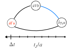
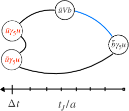
Figure 5: Wick contractions for the $B\to\pi\pi\ell\bar{\nu}$ process. The $B$-meson is located at $t=0$, the interpolating operator for the $\rho$, $\bar{u}\Gamma u$, is located at $\Delta t$ and the current insertion is located at $t_{J}$.

The three-point function contains the information about the matrix elements, $\langle\pi\pi,n|J_{\mu}|B\rangle$:

$$C_{3}^{a}=\sum_{n\in\pi\pi}\sum_{m\in B} Z_{a}^{n}\;\langle n|J_{\mu}|m\rangle\;Z_{B}^{m}\;\frac{e^{-E_{n}(\Delta t-t_{J})}e^{-E_{m}(t_{J})}}{2E_{n}2E_{m}},$$ (6)

the sum $n\in\pi\pi$ is the sum over all the states on the final state, and the sum $m\in B$ is the sum over all the states in the initial state. We are not interested in the excited states in the initial state. As the $B$-meson interpolator describes the ground state well, we can forget the sum over $m\in B$.

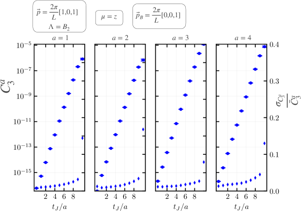
Figure 6: Example three point correlation functions in the irreducible representation $B_{2}$ of the $\vec{P}=\frac{2\pi}{L}(1,0,1)$, with $\vec{p}_{B}=\frac{2\pi}{L}(0,0,1)$. The circles with uncertainties represent the data, while the diamonds show the relative uncertainty of the data.

An example of the three-point correlation functions is shown in Fig. 6, where we show the irreducible representation $B_{2}$ of the $\vec{P}=\frac{2\pi}{L}(1,0,1)$ and a set of four interpolating operators:

$$O_{1}^{B_{2}} =\bar{q}\Gamma_{B_{2}}q,$$ (7)

$$O_{2}^{B_{2}} =\bar{q}\gamma_{t}\Gamma_{B_{2}}q,$$ (8)

$$O_{3}^{B_{2}} =\pi(p_{1})\pi(p_{2}),\text{ and }$$ (9)

$$O_{4}^{B_{2}} =\pi(p_{1}^{\prime})\pi(p_{2}^{\prime}).$$ (10)

These three-point correlation functions still contain the sum over $n$ on the final state - on this side of the three-point correlation function, we also want to get excited state information. To achieve this, we make use of the results from the variational analysis - we construct optimized three-point functions according to [37, 38, 39]:

$$\Omega_{3}^{n}=u_{a}^{n}C_{3}^{a},$$ (11)

where we use one of the crucial aspects of the variational analysis. It allows us to build orthogonal states within our basis, reducing the sum over all the states $n\in\pi\pi$ to a specific state $n$. By using the relation:

$$u_{a}^{n}Z_{a}^{m}=\sqrt{2E_{n}}e^{E_{n}t_{0}/2}\delta_{nm},$$ (12)

the sum in Eq. 11 reduces to:

$$\Omega_{3}^{n}=\sqrt{2E_{n}}e^{E_{n}t_{0}/2}\;\langle n|J_{\mu}|B\rangle\;Z_{B}\;\frac{e^{-E_{n}(\Delta t-t_{J})}e^{-E_{B}(t_{J})}}{2E_{n}2E_{B}}.$$ (13)

By simply removing the temporal dependence, we can determine the matrix elements $\langle n|J_{\mu}|B\rangle$ between the initial $B$-meson and the final, $n$-th state in the set of final volume $\pi\pi$ states. Alternatively we can construct a ratio [16],

$$R_{n}=\frac{\Omega_{3}^{n}\bar{\Omega}_{3}^{m}}{C_{B}(\Delta t)\lambda_{n}(\Delta t,t_{0})},$$ (14)

where the $\bar{\Omega_{3}^{n}}$ three-point function has the quark-flows reversed, i.e. is the complex-conjugate of $\Omega_{3}^{n}$. These matrix elements would correspond to the second-to-left-most diagram in bottom half of Fig. 4.

As is the case for the spectroscopy, so is the case for the matrix element analysis - when fitting, we make assumptions of the models, i.e., one-state fits, two-state fits, either on the initial state side or the final state side, as well as fitting both $\Omega_{3}^{n}$ and $R_{n}$ we produce a large number of fits. We employ the Akaike Information Criterion as outlined in Ref. [40] to average over the matrix elements determined in this way properly. In this manner, we produce matrix elements at a specific kinematical point of $E_{n}^{\star}$ and $q^{2}$, as seen in Fig. 7.

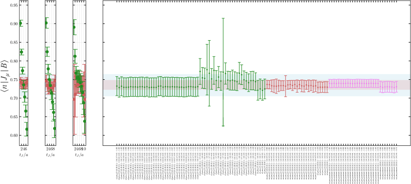
Figure 7: The Akaike Information Criterion matrix element average over all the models. The green-shaded region shows the matrix elements determined from the $\Omega_{3}^{n}$, and the red-shaded region shows the matrix elements determined from the $R_{n}$.

Two values for the matrix elements are determined this way - the green-shaded region, fitted to the $\Omega_{3}^{n}$ data, corresponds to our chosen fit. In contrast, the red-shaded region, fitted to the $R_{n}$ data, corresponds to our systematic fit. In this manner, we include a systematic uncertainty in our determination of the transition amplitude.

The matrix elements determined on the lattice are affected by finite-volume effects - an effect first pointed out by Lellouch and Lüscher in their seminal work [41], where they derived the normalization factor for the $K\to\pi\pi$ matrix element. The calculation and the effects of the Lellouch-Lüscher normalization factor have been discussed in large detail in Ref. [42] and references therein, however the primary strategy was to tune kinematics (volumes and pion masses) to maximize the size of the matrix element. In Ref. [43] Briceño, Hansen, and Walker-Loud derived the finite-volume effects from a Quantum Field Theoretical approach; the generalization changed the approach from tuning kinematics to using every possible state in the analysis.

To elaborate on the analysis, we must first discuss the transition amplitude that enters the matrix element in the infinite volume. The infinite-volume matrix element obeys a Lorentz decomposition, which for the vector current of the $B\to\pi\pi\ell\bar{\nu}$ looks like:

$$\langle n|J_{\mu}|B\rangle_{\infty}=\frac{2iV(E^{\star},q^{2})}{m_{B}+2m_{\pi}}\epsilon_{\mu\nu\alpha\beta}\,\varepsilon^{\nu*}\,P^{\alpha}p_{B}^{\beta},$$ (15)

where $P$ is the final $\pi\pi$ state four-vector, $\varepsilon$ is the polarization four-vector of the $\pi\pi$ state in $P$-wave and $p_{B}$ is the initial state $B$-meson four vector. The momentum transfer vector $q_{\mu}=P_{\mu}-(p_{B})_{\mu}$ and the momentum transfer is $q^{2}=q_{\mu}q^{\mu}$; $\epsilon$ is the $4$-d Levi-Civita tensor. The quantity $V(E^{\star},q^{2})$ is the transition amplitude and can be written down in many ways - however, there are a few requirements: unitarity and analyticity. Both are satisfied if we write $V$ as:

$$V(E^{\star},q^{2})=F(E^{\star},q^{2})\frac{T(E^{\star})}{k},$$ (16)

where $k$ is the $\pi\pi$ scattering momentum, $T$ is the scattering amplitude and $F$ is new function which we will call the form-factor. For the scattering amplitude $T$ we use the parameterizations from Ref. [29], and for the form factor $F$ we use a generalized $z$-expansion [16]:

$$F(E^{\star},q^{2})=\frac{1}{1-\frac{q^{2}}{m_{P}^{2}}}\sum_{n,m}A_{n,m}\,z^{n}(q^{2})\,(E^{\star 2}-E_{thr}^{2})^{m},$$ (17)

where $E_{thr}=2m_{\pi}$. To relate the infinite-volume matrix element with the finite-volume matrix element, we recall the two-point correlation function in a finite-volume being expanded as a sum of poles, where the poles are located at the finite-volume energies. Nevertheless, an expansion over poles involves the pole location, $E_{n}^{\star}$, and the pole residuum $R_{n}$. While the location describes the finite-volume energies, the residue $R_{n}$ describes the normalization of the state belonging to that pole:

$$\langle n|J_{\mu}|B\rangle_{L}=\sqrt{R_{n}}\langle n|J_{\mu}|B\rangle_{\infty}.$$ (18)

The residue $R_{n}$ is defined as:

$$R_{n}\,=\lim_{E^{\star}\to E_{n}^{\star}}\frac{E^{\star}-E_{n}^{\star}}{F^{-1}+T},$$ (19)

while the details of the best way to calculate the residue are discussed in Ref. [44]. To fit the transition amplitude to the lattice data, we thus pick a model for the infinite-volume transition amplitude and calculate the finite-volume matrix element according to Eq. 18. We build a $\chi^{2}$ function from there, which we minimize. For the model transitions amplitudes, we use two types of the scattering amplitudes $T$, $BWI$ - a simple Breit-Wigner, and $BWII$ - a simple Breit-Wigner modified by Blatt-Weisskopf [45] barrier factors. For the form factors $F$, we use $4$ models, that truncate the $z$-expansion at $n=1$ and $m=1$ as listed in Tab. 1

model	$n_{max}$	$m_{max}$	$\chi^{2}/{\rm dof}$
BWI + N0M0	$0$	$0$	$1.18$
BWI + N1M0	$1$	$0$	$1.07$
BWI + N0M1	$0$	$1$	$0.63$
BWI + N0M0	$1$	$1$	$0.50$
BWII + N0M0	$0$	$0$	$0.55$
BWII + N1M0	$1$	$0$	$0.55$
BWII + N0M1	$0$	$1$	$0.52$
BWII + N0M0	$1$	$1$	$0.51$

Table 1: Results of fits to $8$ different models of the $B\to\pi\pi\ell\bar{\nu}$ transition amplitude. The left column lists the model for the scattering amplitude + the model for the form factor. In the middle two columns, the truncation limits of the sum in Eq. 17 are listed, and the right-most column shows the $\chi^{2}/{\rm dof}$.

The average of all the $F$’s combined is shown in Fig. 8, where the dark-shaded region represents the statistical uncertainty, while the light-shaded region represents the systematical uncertainty. The 3-D representation is shown in Fig. 9 for the transition amplitude BWII + N1M1, where the curve shows the fitted transition amplitude. At the same time, the rectangles represent the data with statistical uncertainties only (mapped into the infinite volume).

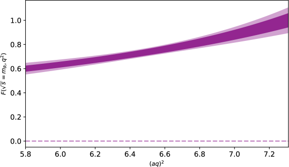
Figure 8: The average of all form factors; the dark-shaded region represents the statistical uncertainty, while the light-shaded region represents the systematical uncertainty.

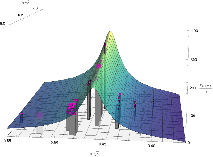
Figure 9: A 3-D plot for the transition amplitude; shown is the scattering amplitude BWII + N1M1, while the histogram points are the data with statistical uncertainties only.

4 Prospects for the Near Future

The prospects in applying the formalism discussed here span Electroweak physics and Photoproduction. While photoproduction processes might not initially appear central to high-energy and nuclear physics, they offer crucial insights into the least understood aspects of the Standard Model, particularly the structure and contents of hadronic resonances. The ongoing debate over the nature of various hadronic resonances, such as the $a_{0}(980)$, $f_{0}(980)$, $D_{0}^{\star}(2400)$, and $D_{s0}^{\star}(2317)$, extends beyond just their masses and decay widths. Comprehensive understanding requires additional data, where lattice QCD, supported by experimental evidence, can contribute significantly. This approach aims to foster a chemistry-like comprehension of hadrons underpinned by theoretical predictions, experimental validations, and intuitive models. Lattice QCD can play a pivotal role in determining radiative transitions in these states, guiding experimental measurements, and extending our knowledge to yet unmeasured quantities such as form factors and other structure observables [46, 47, 48] of resonances.

Numerous experimentally observed processes in Flavor physics await further theoretical backing from lattice QCD. Notable among these are the $b\to s\ell\ell$ transitions, extensively measured by Belle II, LHCb, CMS, and ATLAS [49, 50, 51, 52]. Key processes include $B\to K^{\star}(892)\ell\ell$ and $B\to K_{0}^{\star}(700)\ell\ell$, along with transitions linked to the determination of $V_{ub}$, such as $B\to\rho\ell\bar{\nu}$ and $B\to f_{0}(500)\ell\bar{\nu}$. Their charm quark analogs, like $D\to\rho\ell\bar{\nu}$ and $D\to K^{\star}(892)\ell\bar{\nu}$, also present opportunities for precision tests that could reveal new physics. The $B\to D\pi\ell\bar{\nu}$ process, offering insights into the $B\to D^{\star\star}\ell\bar{\nu}$ puzzle [53] and the inclusive vs exclusive debate over $V_{c}b$, is another area where lattice QCD could significantly contribute. Due to the very narrow nature of the $D^{\star}$ meson, the finite-volume effects in $B\to D^{\star}\ell\bar{\nu}$ are tiny (sub percent according to limits in App. B of Ref. [21]).

While each mesonic process outlined above has a partner baryon process, the situation is different. The processes related to the $b\to s\ell\ell$ have undergone a first iteration [54, 55, 56, 57], and improvements are planned [58]; however, some of the final states are hadronically unstable and will inevitably require the utilization of the finite-volume formalism in the analysis. This poses a challenge, considering spectroscopy studies in the baryon sector lag behind those in the meson sector. On the topic of nucleon transitions, there are essential and exciting processes related to the $\Delta(1232)$. At first, it would be great to see a similar program for the $\Delta(1232)$ as was seen for the $\rho$ resonance; this would provide us with sufficient confidence to determine also the transition amplitudes for $N\gamma\to\Delta(1232)$ and the $N(V-A)\to\Delta(1232)$, which will play a crucial role in the event simulation and identification at DUNE [26].

5 Summary

The study of electroweak transitions is crucial for understanding particle behavior, especially in processes altering quark flavor or lepton number. These transitions not only enrich our understanding of the Standard Model, particularly in aspects like the Standard Model parameters, but also explore CP violation and the matter-antimatter asymmetry of the universe and use rare decays as probes for Physics Beyond the Standard Model. Lattice Quantum Chromodynamics (QCD) has been vital in determining the elements of the CKM matrix thus far. However, a gap remains in the study of hadronic resonances, opening an opportunity for many new processes.

The finite-volume lattice QCD methodology involves complex computational techniques to determine infinite-volume transition amplitudes, encompassing spectrum and matrix element analysis. However, both aspects have matured sufficiently that any collaboration can pick them up and utilize them in phenomenological calculations of their choice. Furthermore, to those who still need more confidence, try, and if you get stuck, know that you are in an open community that always welcomes questions.

References

- [1] Flavour Lattice Averaging Group (FLAG) Collaboration, Y. Aoki et al., “FLAG Review 2021,” Eur. Phys. J. C 82 no. 10, (2022) 869, arXiv:2111.09849 [hep-lat].
- [2] S. Wehle, Angular Analysis of and Search for at the Belle Experiment. PhD thesis, Hamburg U., Hamburg, 2016.
- [3] Particle Data Group Collaboration, R. L. Workman et al., “Review of Particle Physics,” PTEP 2022 (2022) 083C01.
- [4] RBC, UKQCD Collaboration, Z. Bai et al., “Standard Model Prediction for Direct CP Violation in K→ Decay,” Phys. Rev. Lett. 115 no. 21, (2015) 212001, arXiv:1505.07863 [hep-lat].
- [5] RBC, UKQCD Collaboration, R. Abbott et al., “Direct CP violation and the rule in decay from the standard model,” Phys. Rev. D 102 no. 5, (2020) 054509, arXiv:2004.09440 [hep-lat].
- [6] RBC, UKQCD Collaboration, T. Blum, P. A. Boyle, D. Hoying, T. Izubuchi, L. Jin, C. Jung, C. Kelly, C. Lehner, A. Soni, and M. Tomii, “I=3/2 and I=1/2 channels of K→ decay at the physical point with periodic boundary conditions,” Phys. Rev. D 108 no. 9, (2023) 094517, arXiv:2306.06781 [hep-lat].
- [7] N. Ishizuka, K. I. Ishikawa, A. Ukawa, and T. Yoshié, “Calculation of decay amplitudes with improved Wilson fermion action in non-zero momentum frame in lattice QCD,” Phys. Rev. D 98 no. 11, (2018) 114512, arXiv:1809.03893 [hep-lat].
- [8] Hadron Spectrum Collaboration, M. Peardon, J. Bulava, J. Foley, C. Morningstar, J. Dudek, R. G. Edwards, B. Joo, H.-W. Lin, D. G. Richards, and K. J. Juge, “A Novel quark-field creation operator construction for hadronic physics in lattice QCD,” Phys. Rev. D 80 (2009) 054506, arXiv:0905.2160 [hep-lat].
- [9] NA48 Collaboration, A. Lai et al., “A Precise measurement of the direct CP violation parameter Re(),” Eur. Phys. J. C 22 (2001) 231–254, arXiv:hep-ex/0110019.
- [10] KTeV Collaboration, E. T. Worcester, “The Final Measurement of Epsilon-prime/Epsilon from KTeV,” in Heavy Quarks and Leptons 2008 (HQ&L08). 9, 2009. arXiv:0909.2555 [hep-ex].
- [11] K. Aoki et al., “Extension of the J-PARC Hadron Experimental Facility: Third White Paper,” arXiv:2110.04462 [nucl-ex].
- [12] KOTO Collaboration, H. Nanjo, “KOTO II at J-PARC : toward measurement of the branching ratio of ,” J. Phys. Conf. Ser. 2446 no. 1, (2023) 012037.
- [13] NA62, KLEVER Collaboration, “Rare decays at the CERN high-intensity kaon beam facility,” arXiv:2009.10941 [hep-ex].
- [14] “Towards hadronic d decays at the su(3) flavour symmetric point,” https://indico.fnal.gov/event/57249/contributions/271297/. Accessed: 2023-12-30.
- [15] R. A. Briceño, J. J. Dudek, R. G. Edwards, C. J. Shultz, C. E. Thomas, and D. J. Wilson, “The amplitude and the resonant transition from lattice QCD,” Phys. Rev. D 93 no. 11, (2016) 114508, arXiv:1604.03530 [hep-ph]. [Erratum: Phys.Rev.D 105, 079902 (2022)].
- [16] C. Alexandrou, L. Leskovec, S. Meinel, J. Negele, S. Paul, M. Petschlies, A. Pochinsky, G. Rendon, and S. Syritsyn, “ transition and the radiative decay width from lattice QCD,” Phys. Rev. D 98 no. 7, (2018) 074502, arXiv:1807.08357 [hep-lat]. [Erratum: Phys.Rev.D 105, 019902 (2022)].
- [17] M. Niehus, M. Hoferichter, and B. Kubis, “The anomaly from lattice QCD and dispersion relations,” JHEP 12 (2021) 038, arXiv:2110.11372 [hep-ph].
- [18] Hadron Spectrum Collaboration, A. Radhakrishnan, J. J. Dudek, and R. G. Edwards, “Radiative decay of the resonant K* and the K→K amplitude from lattice QCD,” Phys. Rev. D 106 no. 11, (2022) 114513, arXiv:2208.13755 [hep-lat].
- [19] D. J. Wilson, R. A. Briceno, J. J. Dudek, R. G. Edwards, and C. E. Thomas, “Coupled scattering in -wave and the resonance from lattice QCD,” Phys. Rev. D 92 no. 9, (2015) 094502, arXiv:1507.02599 [hep-ph].
- [20] H. B. Meyer, “Lattice QCD and the Timelike Pion Form Factor,” Phys. Rev. Lett. 107 (2011) 072002, arXiv:1105.1892 [hep-lat].
- [21] R. A. Briceño and M. T. Hansen, “Multichannel 0 2 and 1 2 transition amplitudes for arbitrary spin particles in a finite volume,” Phys. Rev. D 92 no. 7, (2015) 074509, arXiv:1502.04314 [hep-lat].
- [22] A. Accardi et al., “Strong Interaction Physics at the Luminosity Frontier with 22 GeV Electrons at Jefferson Lab,” arXiv:2306.09360 [nucl-ex].
- [23] PANDA Collaboration, G. Barucca et al., “PANDA Phase One,” Eur. Phys. J. A 57 no. 6, (2021) 184, arXiv:2101.11877 [hep-ex].
- [24] Belle-II Collaboration, F. Abudinén et al., “Reconstruction of decays identified using hadronic decays of the recoil meson in 2019 – 2021 Belle II data,” arXiv:2211.15270 [hep-ex].
- [25] Belle Collaboration, C. Beleño et al., “Measurement of the branching fraction of the decay in fully reconstructed events at Belle,” Phys. Rev. D 103 no. 11, (2021) 112001, arXiv:2005.07766 [hep-ex].
- [26] NuSTEC Collaboration, L. Alvarez-Ruso et al., “NuSTEC White Paper: Status and challenges of neutrino–nucleus scattering,” Prog. Part. Nucl. Phys. 100 (2018) 1–68, arXiv:1706.03621 [hep-ph].
- [27] L. A. Ruso et al., “Theoretical tools for neutrino scattering: interplay between lattice QCD, EFTs, nuclear physics, phenomenology, and neutrino event generators,” arXiv:2203.09030 [hep-ph].
- [28] D. Simons, N. Steinberg, A. Lovato, Y. Meurice, N. Rocco, and M. Wagman, “Form factor and model dependence in neutrino-nucleus cross section predictions,” arXiv:2210.02455 [hep-ph].
- [29] C. Alexandrou, L. Leskovec, S. Meinel, J. Negele, S. Paul, M. Petschlies, A. Pochinsky, G. Rendon, and S. Syritsyn, “-wave scattering and the resonance from lattice QCD,” Phys. Rev. D 96 no. 3, (2017) 034525, arXiv:1704.05439 [hep-lat].
- [30] M. Luscher, “Two particle states on a torus and their relation to the scattering matrix,” Nucl. Phys. B 354 (1991) 531–578.
- [31] C. h. Kim, C. T. Sachrajda, and S. R. Sharpe, “Finite-volume effects for two-hadron states in moving frames,” Nucl. Phys. B 727 (2005) 218–243, arXiv:hep-lat/0507006.
- [32] K. Rummukainen and S. A. Gottlieb, “Resonance scattering phase shifts on a nonrest frame lattice,” Nucl. Phys. B 450 (1995) 397–436, arXiv:hep-lat/9503028.
- [33] L. Leskovec and S. Prelovsek, “Scattering phase shifts for two particles of different mass and non-zero total momentum in lattice QCD,” Phys. Rev. D 85 (2012) 114507, arXiv:1202.2145 [hep-lat].
- [34] R. A. Briceno, “Two-particle multichannel systems in a finite volume with arbitrary spin,” Phys. Rev. D 89 no. 7, (2014) 074507, arXiv:1401.3312 [hep-lat].
- [35] R. A. Briceno, J. J. Dudek, and R. D. Young, “Scattering processes and resonances from lattice QCD,” Rev. Mod. Phys. 90 no. 2, (2018) 025001, arXiv:1706.06223 [hep-lat].
- [36] Hadron Spectrum Collaboration, A. J. Woss, D. J. Wilson, and J. J. Dudek, “Efficient solution of the multichannel Lüscher determinant condition through eigenvalue decomposition,” Phys. Rev. D 101 no. 11, (2020) 114505, arXiv:2001.08474 [hep-lat].
- [37] J. J. Dudek, R. Edwards, and C. E. Thomas, “Exotic and excited-state radiative transitions in charmonium from lattice QCD,” Phys. Rev. D 79 (2009) 094504, arXiv:0902.2241 [hep-ph].
- [38] D. Bečirević, M. Kruse, and F. Sanfilippo, “Lattice QCD estimate of the c (2S) → J/ decay rate,” JHEP 05 (2015) 014, arXiv:1411.6426 [hep-lat].
- [39] C. J. Shultz, J. J. Dudek, and R. G. Edwards, “Excited meson radiative transitions from lattice QCD using variationally optimized operators,” Phys. Rev. D 91 no. 11, (2015) 114501, arXiv:1501.07457 [hep-lat].
- [40] W. I. Jay and E. T. Neil, “Bayesian model averaging for analysis of lattice field theory results,” Phys. Rev. D 103 (2021) 114502, arXiv:2008.01069 [stat.ME].
- [41] L. Lellouch and M. Lüscher, “Weak transition matrix elements from finite volume correlation functions,” Commun. Math. Phys. 219 (2001) 31–44, arXiv:hep-lat/0003023.
- [42] C. J. D. Lin, G. Martinelli, C. T. Sachrajda, and M. Testa, “ decays in a finite volume,” Nucl. Phys. B 619 (2001) 467–498, arXiv:hep-lat/0104006.
- [43] R. A. Briceño, M. T. Hansen, and A. Walker-Loud, “Multichannel 1 2 transition amplitudes in a finite volume,” Phys. Rev. D 91 no. 3, (2015) 034501, arXiv:1406.5965 [hep-lat].
- [44] R. A. Briceño, J. J. Dudek, and L. Leskovec, “Constraining coupled-channel amplitudes in finite-volume,” Phys. Rev. D 104 no. 5, (2021) 054509, arXiv:2105.02017 [hep-lat].
- [45] F. Von Hippel and C. Quigg, “Centrifugal-barrier effects in resonance partial decay widths, shapes, and production amplitudes,” Phys. Rev. D 5 (1972) 624–638.
- [46] R. A. Briceño, M. T. Hansen, and A. W. Jackura, “Consistency checks for two-body finite-volume matrix elements: I. Conserved currents and bound states,” Phys. Rev. D 100 no. 11, (2019) 114505, arXiv:1909.10357 [hep-lat].
- [47] R. A. Briceño, M. T. Hansen, and A. W. Jackura, “Consistency checks for two-body finite-volume matrix elements: II. Perturbative systems,” Phys. Rev. D 101 no. 9, (2020) 094508, arXiv:2002.00023 [hep-lat].
- [48] R. A. Briceño, A. W. Jackura, F. G. Ortega-Gama, and K. H. Sherman, “On-shell representations of two-body transition amplitudes: Single external current,” Phys. Rev. D 103 no. 11, (2021) 114512, arXiv:2012.13338 [hep-lat].
- [49] Belle-II Collaboration, F. Abudinén et al., “Measurement of the branching fraction for the decay at Belle II,” arXiv:2206.05946 [hep-ex].
- [50] LHCb Collaboration, R. Aaij et al., “Angular Analysis of the Decay,” Phys. Rev. Lett. 126 no. 16, (2021) 161802, arXiv:2012.13241 [hep-ex].
- [51] CMS Collaboration, A. M. Sirunyan et al., “Angular analysis of the decay B+ K∗(892) in proton-proton collisions at 8 TeV,” JHEP 04 (2021) 124, arXiv:2010.13968 [hep-ex].
- [52] ATLAS Collaboration, M. Aaboud et al., “Angular analysis of decays in collisions at TeV with the ATLAS detector,” JHEP 10 (2018) 047, arXiv:1805.04000 [hep-ex].
- [53] E. J. Gustafson, F. Herren, R. S. Van de Water, R. van Tonder, and M. L. Wagman, “A model independent description of decays,” arXiv:2311.00864 [hep-ph].
- [54] S. Meinel and G. Rendon, “ form factors from lattice QCD,” Phys. Rev. D 103 no. 7, (2021) 074505, arXiv:2009.09313 [hep-lat].
- [55] S. Meinel and G. Rendon, “form factors from lattice QCD,” Phys. Rev. D 103 no. 9, (2021) 094516, arXiv:2103.08775 [hep-lat].
- [56] S. Meinel and G. Rendon, “c→*(1520) form factors from lattice QCD and improved analysis of the b→*(1520) and b→c*(2595,2625) form factors,” Phys. Rev. D 105 no. 5, (2022) 054511, arXiv:2107.13140 [hep-lat].
- [57] C. Farrell and S. Meinel, “Form factors for the charm-baryon semileptonic decay from domain-wall lattice QCD,” in 40th International Symposium on Lattice Field Theory. 9, 2023. arXiv:2309.08107 [hep-lat].
- [58] S. Meinel, “Status of next-generation form-factor calculations,” in 40th International Symposium on Lattice Field Theory. 9, 2023. arXiv:2309.01821 [hep-lat].