Identifying thermal effects in neutron star merger remnants with model-agnostic waveform reconstructions and third-generation detectors

Abstract

We explore the prospects for identifying differences in simulated gravitational-wave signals of binary neutron star (BNS) mergers associated with the way thermal effects are incorporated in the numerical-relativity modelling. We consider a hybrid approach in which the equation of state (EoS) comprises a cold, zero temperature, piecewise-polytropic part and a thermal part described by an ideal gas, and a tabulated approach based on self-consistent, microphysical, finite-temperature EoS. We use time-domain waveforms corresponding to BNS merger simulations with four different EoS. Those are injected into Gaussian noise given by the sensitivity of the third-generation detector Einstein Telescope and reconstructed using BayesWave, a Bayesian data-analysis algorithm that recovers the signals through a model-agnostic approach. The two representations of thermal effects result in frequency shifts of the dominant peaks in the spectra of the post-merger signals, for both the quadrupole fundamental mode and the late-time inertial modes. For some of the EoS investigated those differences are large enough to be told apart, especially in the early post-merger phase when the signal amplitude is the loudest.

I Introduction

We are in a golden era of astrophysics where a plethora of new gravitational wave (GW) observations is changing our understanding of the Universe at an unprecedented rate Abbott et al. (2019a); Abbott et al. (2021); The LIGO Scientific Collaboration et al. (2021); Abbott et al. (2023). In particular, the observations of GWs from the first binary neutron star (BNS) merger – event GW170817 – along with its post-merger emission of electromagnetic (EM) radiation, spurred the era of multimessenger astronomy (Abbott et al., 2017a; Abbott et al., 2017b; Abbott et al., 2017c). This single event provided: i) the most direct evidence that stellar compact mergers, where at least one of the binary companions is a neutron star (NS), are progenitors of the central engines that power short gamma-ray bursts (sGRBs); ii) strong observational support to theoretical proposals linking BNS mergers with production sites for r-process nucleosynthesis and kilonovae (Li and Paczynski, 1998; Metzger, 2017; Troja et al., 2017; Kasen et al., 2017); iii) an independent measure for the expansion of the Universe (Abbott et al., 2017a; Dietrich et al., 2020); and iv) tight constraints on the equation of state (EoS) of matter at supranuclear densities (Rezzolla et al., 2018; Ruiz et al., 2018; Shibata et al., 2017; Margalit and Metzger, 2017; Abbott et al., 2018; Abbott et al., 2019b).

From the GW observation point of view, most of the results inferred from the analysis of GW170817 are based on the late inspiral part of the waveform. During this period, tidal forces are inefficient to transfer energy and angular momentum from the orbit to the NS, and hence the stars can be regarded as having effectively zero temperature. Following merger, however, shock heating rises up the temperature of the remnant to $\gtrsim 10$ MeV. Such high temperatures provide an additional pressure support that may change the internal structure of the remnant and its subsequent evolution. It is expected that observations of post-merger GWs, presently at the limit of the technology used in second-generation detectors Abbott et al. (2017b), will yield new insights on the nuclear EoS of NS at finite temperature.

GW searches of BNS mergers and inference of source parameters rely on accurate waveform models for the inspiral signal. Those are based on analytical relativity (computing waveform approximants using post-Newtonian expansions or the effective-one-body approach Lackey et al. (2017); Narikawa and Uchikata (2022)) and numerical relativity, the full-fledged numerical solution of Einstein’s field equations coupled to the equations describing NS matter and radiation processes (see e.g. Sun et al. (2022); Foucart et al. (2023, 2020); Gieg et al. (2022); Hayashi et al. (2022); Radice et al. (2022)). In numerical simulations of BNS mergers thermal effects are incorporated using two alternative approaches. The first one is a “hybrid approach” which assumes that the pressure and the internal energy have two contributions, namely a cold, zero temperature part described by a polytropic EoS (or a family of piecewise polytropes) and a thermal part described by an ideal-gas-like EoS (Janka et al., 1993; Dimmelmeier et al., 2002; Shibata et al., 2005). The latter is given by $P_{\rm th}=\rho_{0}\,\epsilon_{\rm th}(\Gamma_{\rm th}-1)$, with $\rho_{0}$ the rest-mass density, and $P_{\rm th}$ and $\epsilon_{\rm th}$ the thermal pressure and thermal energy density, respectively, and $\Gamma_{\rm th}$ the adiabatic index, a constant that lays in the range $1\lesssim\Gamma_{\rm th}\lesssim 2$ for causality constraints, but that in typical BNS merger simulations is set between $1.6$ and $2$ (see e.g. (Constantinou et al., 2015; Takami et al., 2015)). The second approach employs tabulated representations of microphysical finite-temperature EoS, providing a self-consistent method to probe the impact of thermal effects in the merger dynamics. Although the hybrid approach is computationally preferred, it has some limitations. In particular, it has been shown that the value of the thermal adiabatic index $\Gamma_{\rm th}$ above half saturation density strongly depends on the nucleon effective mass (Lim and Holt, 2019). Therefore, it is likely that this approach overestimates the thermal pressure by a few orders of magnitude (Raithel et al., 2021), which may induce significant changes in the GW frequencies (Bauswein et al., 2010; Figura et al., 2021). As the tabulated approach incorporates the temperature self-consistently the above issue is not present. BNS merger simulations based on tabulated EoS, while computationally more challenging than those based on the hybrid approach, are becoming increasingly more common  (Oechslin et al., 2007; Bauswein et al., 2010; Sekiguchi et al., 2011; Fields et al., 2023; Espino et al., 2022; Werneck et al., 2023; Guerra et al., 2024). These two alternative ways of including thermal effects in the numerical simulations results in measurable differences in the GW signal, especially in the post-merger part, significantly affecting the frequency spectra (see e.g. Bauswein et al. (2010); Guerra et al. (2024)).

During the first $\sim 5\,\rm ms$ after merger, nonaxisymmetric deformations of the remnant are accompanied by the emission of high-frequency GWs. The frequency spectra is characterized by the presence of distinctive peaks associated with oscillation modes due to nonlinear interactions between the quadrupole and quasi-radial modes, and the rotation of the nonaxisymmetric binary remnant. These peaks are typically denoted as $f_{2\pm 0}$, $f_{\rm spiral}$, and $f_{2}$ (or $f_{\rm peak}$)  Stergioulas et al. (2011); Hotokezaka et al. (2013); Bauswein and Stergioulas (2015); Takami et al. (2015); Bauswein et al. (2016); Bauswein and Stergioulas (2019). As pointed out in Rezzolla and Takami (2016) the frequency of the $f_{2}$ mode changes by around $\sim 5\%$ in time. These (initial) frequency values are denoted as $f_{2,i}$ to distinguish them from the value of $f_{2}$ reached during the quasi-stationary evolution of the GW signal. Through the analysis of these peaks, inference on NS properties may be possible. In particular, it has been shown that their frequencies are related quasi-universally with the tidal deformability of the stars, and the maximum-mass of non-rotating configurations (Read et al., 2013; Bauswein and Stergioulas, 2015; Takami et al., 2015; Rezzolla and Takami, 2016; Guerra et al., 2024; Topolski et al., 2023).

Long-term simulations of the post-merger remnant extending beyond $\sim 50$ ms have also revealed the appearance of inertial modes (De Pietri et al., 2018, 2020). Their GWs dominate over those associated with the initial $f_{2}$ mode at late post-merger times, but have lower frequencies and amplitudes. As inertial modes depend on the rotation rate of the star and on its thermal stratification, their detection in GWs would provide a unique opportunity to probe the rotational and thermal states of the merger remnant (see e.g. Kastaun (2008)).

Recently, long-term simulations of BNS mergers exploring the influence of the treatment of the thermal part of the EoS by comparing models using hybrid and tabulated approaches have been reported in Guerra et al. (2024). The differences found in the dynamics and GW emission can be used to gauge the importance of the numerical treatment of thermal effects in the EoS, which has observational implications. In this work, we investigate the identification of such differences in BNS merger remnants by reconstructing the GW signals of Guerra et al. (2024) using BayesWave Cornish and Littenberg (2015); Littenberg and Cornish (2015), a Bayesian data-analysis algorithm that recovers the post-merger signal through a morphology-independent approach using series of sine-Gaussian wavelets. We stress that our simulations focus on the possible identification of a single difference in the post-merger remnant – the implementation of thermal effects in the EoS – and thus assume that potential effects from neglected ingredients in the modelling (e.g. magnetic fields, viscosity, neutrinos or the knowledge of the underlying nuclear interaction) would be identical in both setups. This investigation is a follow-up of our recent work in Miravet-Tenés et al. (2023), where we first employed BayesWave to analyze the detectability prospects of the inertial modes computed in the simulations of De Pietri et al. (2018, 2020) employing only hybrid BNS models. Moreover, we further extend the analysis of Miravet-Tenés et al. (2023) by studying the identification of differences in the treatment of thermal effects across the entire post-merger signal, i.e. both in the early part where the $f_{2}$ mode dominates and in the late part where inertial modes are excited. As done in Miravet-Tenés et al. (2023), we perform waveform injections corresponding to a set of EoS, each with a hybrid and a tabulated version, into the noise of the third-generation GW detector Einstein Telescope (ET) Punturo et al. (2010); Hild et al. (2011); Maggiore et al. (2020); Branchesi et al. (2023) from BNS sources at different distances. The posterior distributions of the recovered waveforms give us distributions of the peak frequencies, that can be related to physical properties of the merger remnant via empirical relations.

Our analysis is complementary to the recent work reported in Villa-Ortega et al. (2023) where Bayesian model selection was used to explore differences between the hybrid and the tabulated approaches with the same set of GW signals from Guerra et al. (2024). This is a completely different approach to our model-agnostic reconstructions. The findings reported in Villa-Ortega et al. (2023), where differences between tabulated and hybrid treatments of thermal effects were found to lead to differences in the post-merger GW observable by third-generation detectors at source distances $\leq 50$ Mpc, are consistent with what is reported here. We find that differences in the distribution of the main frequency peaks in the post-merger GW spectra in hybrid and tabulated models can be resolved in third-generation detectors up to distances similar to those reported in Villa-Ortega et al. (2023). Recently, the studies in Raithel and Paschalidis (2023) showed that finite-temperature effects included through the hybrid approach can be measurable with future detectors if the cold EoS is well constrained.

The paper is organized as follows: we summarize the setup of the BNS merger simulations of Guerra et al. (2024) in Section II. Next, in Section III we briefly present the BayesWave algorithm and introduce the quantities we use to assess the waveform reconstructions. Our main results are discussed in Section IV. We divide this section in two parts: the first one is focused on the early post-merger signal, where we also discuss different EoS-insensitive fits that relate the $f_{2,i}$ and $f_{2}$ modes with the tidal deformability of neutron stars. Then, in the second part we consider the late post-merger phase and study the differences in the frequencies of the inertial modes for our set of EoS. The conclusions of our work are presented in Section V. Finally, Appendix A contains a brief summary of our findings for source inclinations and sky locations different than those considered in the main body of the paper where optimal orientation and sky location is assumed.

II Summary of the BNS mergers setup

The gravitational waveforms employed in our analysis were computed in the numerical-relativity simulations of BNS mergers recently conducted by Guerra et al. (2024). The initial data for those simulations consist of two equal-mass, irrotational neutron stars modeled by finite-temperature (tabulated) microphysical EoSs, namely DD2 Typel et al. (2010), HShen Shen et al. (2011), LS220 James M. Lattimer (1991), and SLy4 Chabanat et al. (1998). These initial data were built using LORENE Gourgoulhon et al. (2001); Taniguchi and Gourgoulhon (2002); Lor . The EoS tables are obtained following the work of Schneider et al. Schneider et al. (2017) and are freely available at ste . The initial temperature is fixed to $T=0.01\,\rm{MeV}$, the lowest value on the tables. These EoSs span a reasonable range of central densities, radii, and maximum gravitational masses for irrotational neutron stars. The initial separation of the two stars is $44.3\,\rm km$ and the rest-mass of each star is $M_{0}=1.4\,M_{\odot}$. Their properties are summarized in Table 1. For comparison purposes we also consider waveforms obtained in simulations of BNS mergers based on hybrid EoSs, consisting of a cold and a thermal part. The cold component of each EoS is made of piecewise polytropic representations of the above EoSs using a piecewise regression as in Pilgrim (2021) with seven pieces Read et al. (2009). Correspondingly, the thermal component is based on a $\Gamma$-law EoS with a constant adiabatic index $\Gamma_{\rm th}=1.8$.

The two types of BNS models we use – hybrid and tabulated – are built as similar as possible, to minimize the effects of differences that the initial data may have in our study. However, there are intrinsic differences in the way the models are built (e.g. the lowest value of the temperature in the tables is $T=0.01$ MeV, which affects the density distribution at low densities) that make not possible to build the exact same stars. The gravitational mass vs circumferential radius for the two types of configurations and for the four EoS used in this paper are displayed in Fig. 1 with solid red circles. The unavoidable small discrepancy visible in this plot leads to a difference of $\lesssim 10\%$ between the values of the tidal deformability $\Lambda$ of the tabulated and the hybrid EoS listed in Table 1. We refer the reader to Guerra et al. (2024) for further details.

Table 1: Summary of the initial properties of the BNS configurations. We list the EoS, the temperature $T[\rm MeV]$, the gravitational mass $M[M_{\odot}]$, and the compactness $\mathcal{C}\equiv M/R_{\rm eq}$ and the tidal deformability $\Lambda=(2/3)\kappa_{2}\,\mathcal{C}^{-5}$ for each individual star. Here $R_{\rm eq}$ is the equatorial coordinate radius toward the companion of each star, and $\kappa_{2}$ is the second Love number. The ADM mass $M_{\rm ADM}[M_{\odot}]$, the ADM angular momentum $J_{\rm ADM}[M_{\odot}^{2}]$ and the angular velocity $\Omega[\rm krad/s]$, for an initial binary coordinate separation of $\sim 44.3\,\rm km$. In all cases the NS has a rest-mass $M_{0}=1.4M_{\odot}$. The first (last) four rows correspond to the BNSs modeled through a fully-tabulated (piecewise polytropic) EoS. Dash symbol denotes “not applicable”.

EoS	$T$	$M$	$\mathcal{C}$	$\Lambda$	$M_{\rm ADM}$	$J_{\rm ADM}$	$\Omega$
SLy4	0.01	1.28	0.16	536.00	2.54	6.63	1.77
DD2	0.01	1.29	0.14	1098.68	2.56	6.73	1.78
HShen	0.01	1.30	0.13	1804.67	2.58	6.82	1.78
LS220	0.01	1.29	0.15	851.72	2.55	6.68	1.77
SLy4	-	1.28	0.16	511.70	2.54	6.62	1.77
DD2	-	1.29	0.14	1113.92	2.56	6.73	1.78
HShen	-	1.30	0.13	1633.24	2.58	6.82	1.78
LS220	-	1.29	0.15	899.05	2.55	6.69	1.77

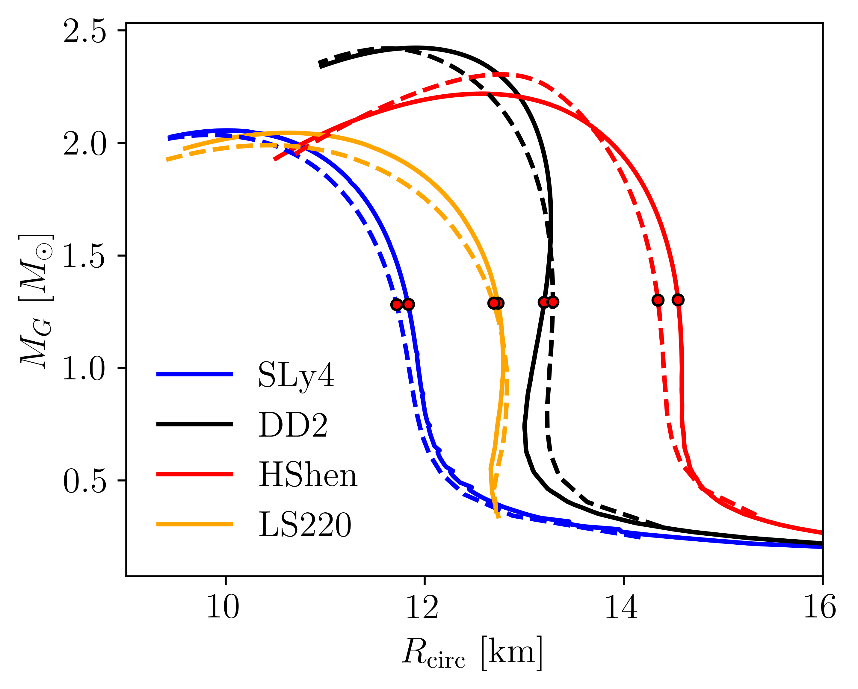
Figure 1: Gravitational mass vs circumferential radius for the tabulated (solid lines) and the hybrid (dotted lines) EoS used in this work. The selected NS configurations are depicted with red dots.

The initial data were evolved in Guerra et al. (2024) using the IllinoisGRMHD code Werneck et al. (2023); Etienne et al. (2015) embedded in the Einstein Toolkit infrastructure Loffler et al. (2012). Much of the numerical infrastructure has been extensively discussed in Werneck et al. (2023); Etienne et al. (2015); Noble et al. (2006); Guerra et al. (2024) to which the interested reader is addressed for details. As a summary we only mention that the code evolves the Baumgarte–Shapiro–Shibata–Nakamura equations Baumgarte and Shapiro (1998); Shibata and Nakamura (1995) coupled to the puncture gauge conditions using fourth-order spatial differentiation. In all cases the damping coefficient appearing in the shift condition was set to 1/$M$ , where $M$ is the ADM mass of the system. Moreover, the IllinoisGRMHD adopts the Valencia formalism for the general relativistic hydrodynamics equations Banyuls et al. (1997); Font (2008) which are integrated with a state-of-the-art finite-volume algorithm. Time integration is performed using the method of lines with a fourth-order Runge-Kutta integration scheme with a Courant-Friedrichs-Lewy (CFL) factor of 0.5.

Some of the evolutions reported in Guerra et al. (2024) extend for over $t-t_{0}\sim 150\,\rm ms$ after merger. This permits to identify the imprint of thermal effects on the post-merger GW signals and in the frequency spectra. In particular, such long-term simulations allow us to study the potential dependence on the treatment of thermal effects for both, the frequencies associated with the fundamental quadrupolar mode, excited about some 5 ms after merger, along with those of inertial models, typically appearing at significantly longer post-merger times De Pietri et al. (2018, 2020); Guerra et al. (2024).

III Waveform reconstruction

III.1 The BayesWave algorithm

The tool we employ to assess possible observational differences in the treatment of thermal effects in the post-merger GW signal is BayesWave Cornish and Littenberg (2015); Littenberg and Cornish (2015), a Bayesian algorithm that uses sine-Gaussian wavelets to reconstruct unmodeled signals with minimal assumptions Bécsy et al. (2017). There are some parameters of the wavelets that the user can fix to optimize the reconstruction. Those appear in the time-domain expression of the wavelets for the “+” and “$\times$” polarizations:

$$h_{+}(t) =Ae^{-(2\pi f_{0}(t-t_{0})/Q)^{2}}\cos{[2\pi f_{0}(t-t_{0})+\phi_{0}]}\,,$$ (1)

$$h_{\times}(t) =\epsilon h_{+}(t)e^{i\pi/2}\,.$$ (2)

In these equations $Q$ is the quality factor, indicating how damped a wavelet is. The algorithm uses a trans-dimensional reversible jump Markov Chain Monte Carlo (RJMCMC) to sample joint posteriors of other parameters of the wavelets, such as their amplitude $A$, their central frequency $f_{0}$, the offset phase $\phi_{0}$, and the ellipticity $\epsilon$. BayesWave also chooses an optimal number of wavelets for the reconstruction, $N_{W}$. The RJMCMC method derives the posterior distribution of the reconstructed waveform and, using the waveform samples, posteriors of quantities that can be derived from the signals are obtained.

III.2 Overlap and Peak Frequency

We employ the overlap function to study the similarity between the recovered model from BayesWave, $h_{r}$, and the injected signal, $h_{i}$:

$$\mathcal{O}=\frac{\langle h_{i},h_{r}\rangle}{\sqrt{\langle h_{i},h_{i}\rangle}\sqrt{\langle h_{r},h_{r}\rangle}}\,.$$ (3)

This expression involves the inner product of two complex quantities, which is defined as

$$\langle a,b\rangle\equiv 2\int_{0}^{\infty}\frac{a(f)b^{*}(f)+a^{*}(f)b(f)}{S_{h}(f)}df\,,$$ (4)

where $S_{h}(f)$ refers to the one-sided noise power spectral density (PSD) of the detector. The asterisk denotes complex conjugation.

The overlap function can take values from -1 to +1. A perfect match between the signals will result in $\mathcal{O}=+1$, and a perfect anti-correlation will give $\mathcal{O}=-1$. If there is no similarity between the signals, the overlap will be 0. Eq. (3) is valid for a single-detector measurement. The expression for the weighted overlap of a network of $N$ detectors is

$$\mathcal{O}_{\rm network}=\frac{\sum^{N}_{k=1}\langle h_{i}^{(k)},h_{r}^{(k)}\rangle}{\sqrt{\sum^{N}_{k=1}\langle h_{i}^{(k)},h_{i}^{(k)}\rangle}\sqrt{\sum^{N}_{k=1}\langle h_{r}^{(k)},h_{r}^{(k)}\rangle}}\,,$$ (5)

where index $k$ stands for the $k$-th detector.

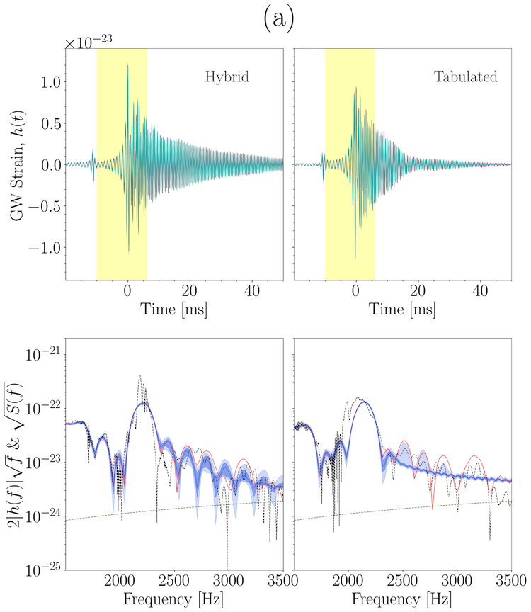
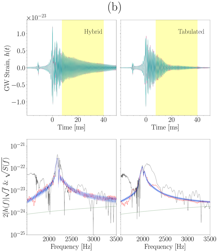
Figure 2: Top row: injected (red) and reconstructed (blue) time-domain waveforms from BNS mergers with the HShen EoS. Bottom row: corresponding ASD, computed either using the complete waveforms (dotted line) or at the time windows depicted in yellow in the strain plots in panels (a) and (b) (see Table 2). The left (right) column of each of the two panels corresponds to the hybrid (tabulated) version of the EoS. The source is located at $D=20$ Mpc. The signals are injected into the ET-D configuration of the ET detector, whose sensitivity curve is shown by the dashed green curve within the frequency range depicted.

From the GW spectra we can analyze the frequency peaks that arise due to the excitation of certain modes of oscillation in the merger remnant. Since the output of BayesWave are time-domain signals, we need to apply the fast Fourier transform (FFT) (Cooley and Tukey, 1965) with a certain time window to study the part of the post-merger phase we are interested in. The FFT is computed using PyCactus Kastaun (2021), a Python package that contains tools for postprocessing data from numerical simulations. Once the spectra are obtained, we look for their frequency peaks. Given the posterior distribution of reconstructed signals, we will end up with a posterior distribution of frequency peaks. Those may be connected to some physical parameters of the merger remnant via empirical relations. We expect the peak frequencies to be located in the range $f\in[1500,4000]$ Hz Chatziioannou et al. (2017); De Pietri et al. (2020). We use this range to set the low-frequency and high-frequency cutoffs for the computation of the overlap and the frequency peaks.

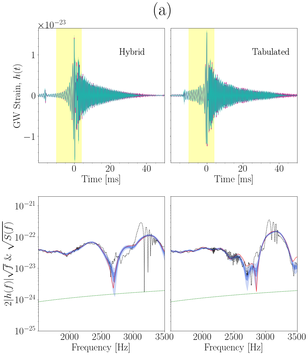
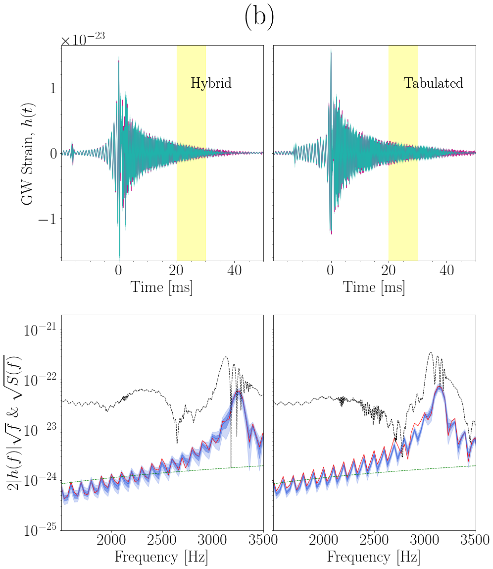
Figure 3: Same as in Figure 2 but for the SLy4 EoS.

IV Results

For all of our injections we use the ET-D configuration from Hild et al. (2011) as the sensitivity curve of the Einstein Telescope (ET), which is formed by a three-detector network on the same site. Our conclusions should also broadly hold for Cosmic Explorer Evans et al. (2021), as its detection capabilities are similar to those of ET. For simplicity and as we did in Miravet-Tenés et al. (2023), we consider Gaussian noise (Blackburn et al., 2008; Abbott et al., 2009; Aasi et al., 2012) (colored by the PSD of the detector) and no sources of noise/glitches are added. The waveforms are injected at different distances, which result in different signal-to-noise ratios (SNRs). We also assume that the source is optimally oriented with respect to the detector. For completeness, in Appendix A we discuss the differences in the overlap function for non-optimal orientation and sky location.

We set a maximum number of wavelets of $N_{W}^{\rm max}=200$, a maximum quality factor of $Q^{\rm max}=200$, $n=2\times 10^{6}$ iterations, and a sampling rate of 8192 Hz, resulting in the same setup used in Miravet-Tenés et al. (2023).

IV.1 Early post-merger phase

We begin by focusing on the first milliseconds after merger. During this early phase, strong non-axisymmetric deformations and nonlinear oscillations are present, namely combinations of oscillation modes and spiral deformations, leading to the emission of GW signals with frequencies around a few kHz. Since the amplitude of these signals is considerably larger than in the late post-merger phase, we also consider correspondingly larger distances, from 1 Mpc up to 200 Mpc.

IV.1.1 Waveform reconstructions

Figures 2 and 3 show the non-whitened, time-domain signal (top panels) and the amplitude spectral density (ASD, bottom panels) of the injected (red) and reconstructed (blue) GW signals (with the detector ASD), at a fixed distance of 20 Mpc. Fig. 2 corresponds to the HShen EoS and Fig. 3 to the SLy4 EoS, respectively. Panels (a) and (b) in both figures differ by the time window used to compute the ASD, highlighted in yellow in the time-domain waveform plots. We adapt the time windows to each particular model and phase of the waveform. The time windows employed for each EoS and phase of the simulation (characterized by a dominant oscillation mode) are summarized in Table 2. The blue-shaded regions in the ASD plots in both figures show the 50% and 90% credible intervals (CIs) of the distribution of the recovered waveforms. These intervals are given by values of the percentiles 25th/75th and 5th/95th, respectively.

The windows used in panel (a) of figures 2 and 3 corresponds to the time interval $t\in[-10,4]$ ms and $t\in[-10,6]$ ms, respectively, being $t=0$ the time of merger. During this phase, the $f_{2,i}$ modes are excited, and they exhibit the frequency peaks shown in the bottom rows. The left column of the panels in both figures show the reconstructions of the hybrid version of the EoS, whereas the right column depicts the tabulated version. For the case of HShen, in panel (a) of Fig. 2, the $f_{2,i}$ peaks are located around 2200 Hz. The ASD of the hybrid and tabulated version of the EoS are similar but the tabulated one produces $f_{2,i}$ modes with a slightly lower frequency. Regarding SLy4, in panel (a) of Fig. 3, the peaks are located around 3250 Hz, and the tabulated version of the EoS also has the peaks at slightly lower frequencies than the hybrid version. The differences between the hybrid and tabulated versions of the EoS are almost negligible, with a difference between the frequency peaks of $\approx 4\%$. For the DD2 and LS220 EoS the mismatch is even smaller.

Table 2: Time windows employed to capture the different oscillation modes appearing during post-merger. Times are expressed in milliseconds and $t=0$ ms is the merger time.

EoS		Mode
	$f_{2,i}$	$f_{2}$	Inertial
SLy4	[-10, 4]	[20, 30]	[75, 140]
DD2	[-10, 4]	[7, 17]	[70, 140]
HShen	[-10, 6]	$[7.5,40]$	[105, 140]
LS220	[-10, 6]	[8, 15]	[80, 140]

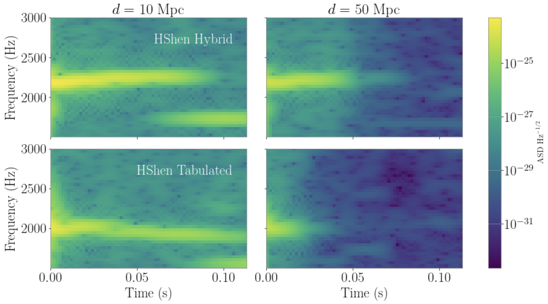
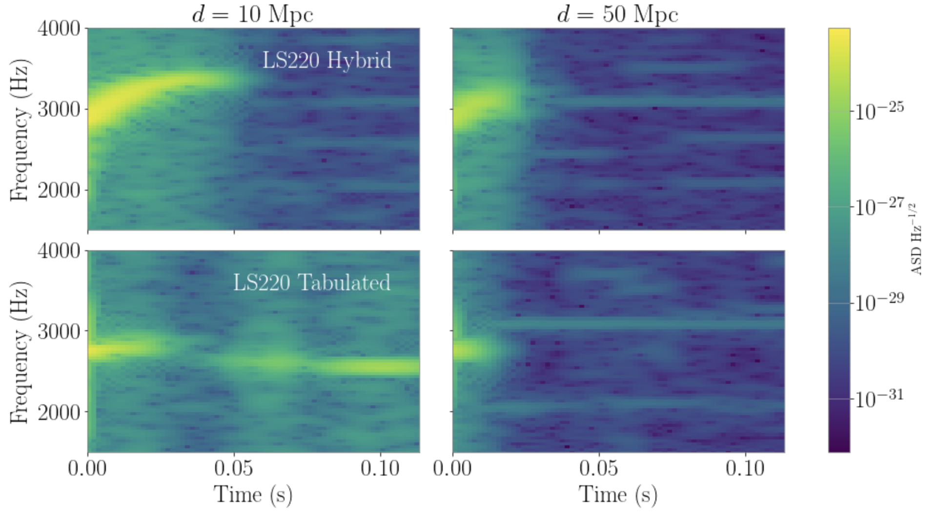
Figure 4: Spectrograms of the reconstructed GW signals at two source distances, $D=10$ Mpc and 50 Mpc. The left (right) panels correspond to the HShen (LS220) EoS. Plots in the upper row depict the hybrid version of the EoS and those in the lower row the tabulated model. As the distance to the source increases, it becomes more difficult to capture the time evolution of the frequency of the signal at late times.

In panels (b) of Figs. 2 and 3 we depict again the time-domain and the spectra of the injected and recovered signals for the same two EoS, but the time window is applied now for the intervals $t\in[7.5,40]$ ms (HShen) and $t\in[20,30]$ ms (SLy4). Therefore, the ASD of the bottom panels show the appearance of the $f_{2}$ modes. For the SLy4 EoS the amplitude of the $f_{2}$ modes is lower than that of the $f_{2,i}$ modes. For the HShen EoS there are more noticeable differences in the position of the peaks between the hybrid and tabulated models than for the SLy4 EoS. For both cases the peaks of the $f_{2}$ modes appear at lower frequencies than for the $f_{2,i}$ modes.

Spectrograms of the median of the reconstructed signals are shown in Figure 4 for the case of HShen (left) and LS220 (right). In both panels, the plots in the upper row refer to the hybrid version of the EoS and the lower row to the tabulated version. This figure shows the spectrograms for two difference source distances, 10 Mpc and 50 Mpc. For a distance of 10 Mpc all the stages of the post-merger signal are visible in the spectrogram of the HShen EoS: there is an initial part where the signal is louder followed by a decrease in frequency and amplitude, visible up to more than 100 ms after merger. This trend occurs for both hybrid and tabulated versions of the HShen EoS. As the distance increases, however, the last part of the signal cannot be reconstructed. Beyond 50 Mpc, the signal is only visible up to $t\sim 50$ ms. Note that, for the hybrid version of the HShen EoS, the signal is detectable for longer times.

The four plots in the right panel of Figure 4 depict two completely different behaviours between the hybrid and tabulated versions of the LS220 EoS. In the first case (upper row), the frequency of the signal increases with time up to $t\sim 40$ ms for sources located at short distances (10 Mpc). At that point, the signal disappears because the remnant collapses to a BH (at $t=66.2$ ms after merger) Guerra et al. (2024). However, the tabulated version of the LS220 EoS (lower row) shows that a stable remnant evolves for more than 100 ms after merger. In this case, the GW signal decreases in amplitude, reaching frequencies of about 2 kHz. At larger source distances (50 Mpc) BayesWave only recovers the inspiral phase and the very early stages after merger, not capturing the collapse of the remnant for the hybrid version of the EoS.

IV.1.2 Frequency peaks of the $f_{2,i}$ and $f_{2}$ modes

From the posterior distributions of the GW signals that BayesWave provides, one can compute the ASD via the FFT of the time-domain signal using a certain time window. This yields posterior distributions of the frequency peaks of the spectra. We start considering time windows spanning from $t\approx 10$ ms before merger to a few tens of milliseconds after merger (depending on the EoS; see Table 2). The size and position of the time windows are chosen to distingish the frequency peaks related to the $f_{2,i}$ and $f_{2}$ modes.

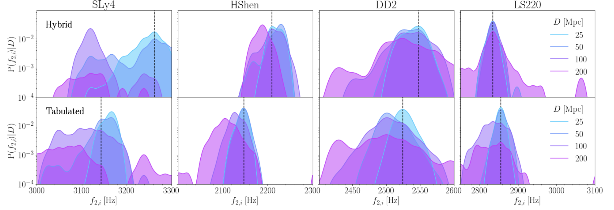
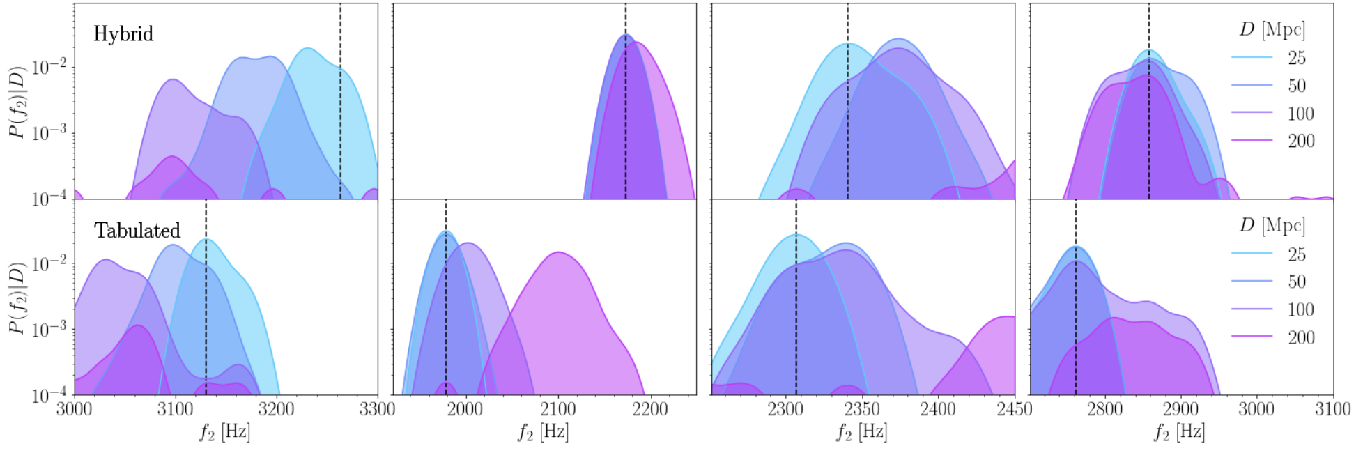
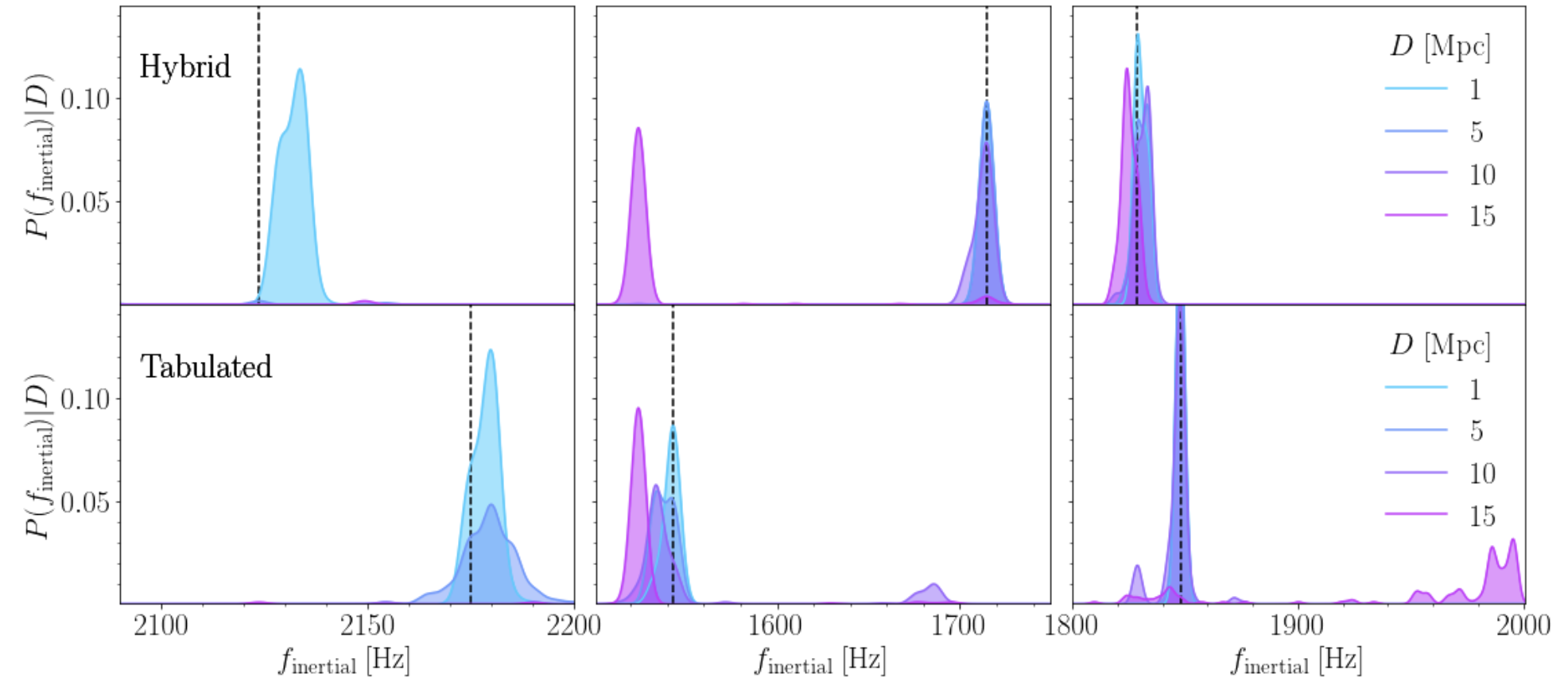
Figure 5: Posterior distributions of the frequency peaks for the $f_{2i}$ modes (top), $f_{2}$ modes (middle), and $f_{\rm inertial}$ modes (bottom). Each column corresponds to a different EoS (SLy4, HShen, DD2 and LS220, from left to right). The upper (lower) rows are the hybrid (tabulated) versions of the corresponding EoS. Each color in the posterior distributions corresponds to a different distance to the source, indicated in the legends. The vertical black dashed lines are the frequency peaks of the injected signals. As expected, the shorter the distance the narrower the distributions and the closer they are to the injected values. We do not show the peaks for LS220 in the bottom row because the hybrid version collapses to a BH and there is no late post-merger signal.

The top and middle panels of Figure 5 show the posterior distributions of the frequency peaks for the $f_{2,i}$ and the $f_{2}$ modes, respectively. (The bottom panel in this figure will be discussed below.) The posterior distributions are constructed using a Gaussian kernel density estimator and setting the bandwidth equal to the frequency resolution given by the FFT (which will be different depending on the time window considered). Each column corresponds to a certain EoS, from left to right SLy4, HShen, DD2 and LS220. The upper row shows the hybrid version of each EoS, and the lower one the tabulated version. The different colors refer to several distances to the source, that range from $D=25$ Mpc to $D=200$ Mpc. For the $f_{2,i}$ mode, shown in the top panel of Figure 5, differences between the treatment of thermal effects in the EoS are only detectable for SLy4 (first column) and HShen (second column). These two EoS show the largest deviation in the frequency peaks as a result of the distinct consideration of thermal effects. The frequency peak of SLy4 is not well recovered for $D\geq 50$ Mpc,with a $p$-value of 0.05 and 0.13 for the hybrid and tabulated cases, respectively, at $D=200$ Mpc. This results in detectable differences between both versions of the EoS only for close enough sources. In the case of DD2 and LS220, the curves of the posterior distributions overlap for all distances, and no differences between the tabulated and hybrid EoS might be seen. The range of detectability is almost the same for all EoS but SLy4 (first column). For the other cases, the peaks are detectable up to $D\gtrsim 200$ Mpc, with $p$-values over 0.15 for all distances.

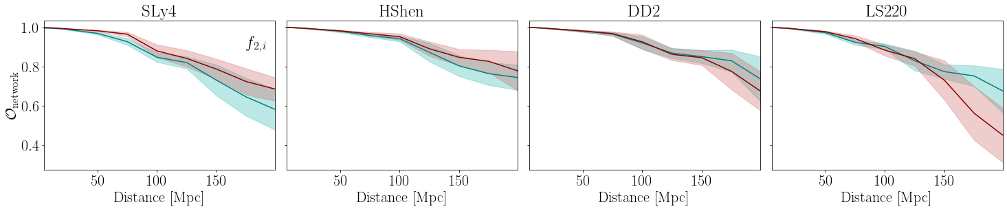
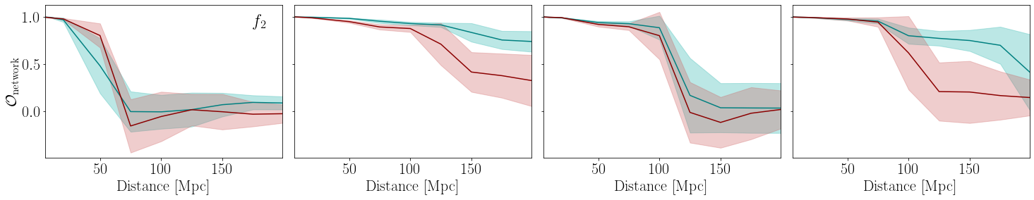
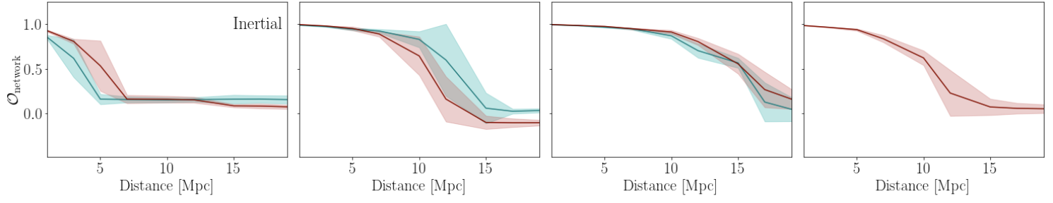
Figure 6: Detector network overlap between the injected and reconstructed signals as a function of the distance to the source. Top, middle and bottom rows correspond to the $f_{2,i}$ modes, the $f_{2}$ modes and the $f_{\rm inertial}$ modes, respectively. Each column corresponds to one EoS. Solid lines indicate the mean value over the waveform posterior distribution and shaded areas are the standard deviations. The blue color corresponds to the hybrid version of the EoS and the red color to the tabulated version. Notice that the blue curve and shaded area are not shown for the LS220 EoS in the bottom-right plot as the remnant for the hybrid version of this EoS collapses to a black hole.

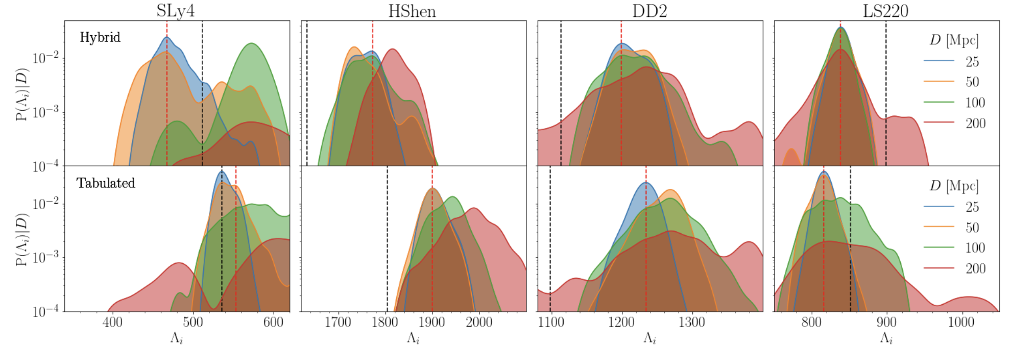
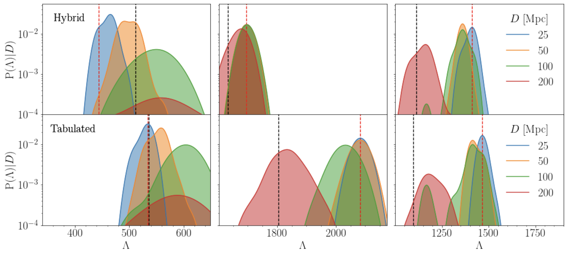
Figure 7: Posterior distributions of the tidal deformability parameter computed from the frequency peaks of the $f_{2,i}$ mode, $\Lambda_{i}$ (top row) and of the $f_{2}$ mode, $\Lambda$ (bottom row). Each column corresponds to a different EoS and different colors correspond to different distances to the source. The vertical red dashed line is the injected value of the parameter (obtained with the fit from Guerra et al. (2024)) and the vertical black dashed line is the true value shown in Table 1 . We do not show the distributions for LS220 in the bottom row because the hybrid version collapses to a BH after the early post-merger phase. See main text for details.

The middle panel of Figure 5 depicts the frequency peaks corresponding to the $f_{2}$ mode. These peaks are more difficult to recover than those of the $f_{2,i}$ mode, even though the differences between the hybrid and tabulated versions of the EoS are more prominent. For SLy4, the recovery is inaccurate for distances $D\gtrsim 50$ Mpc, as the peaks of the posterior distributions are at significantly lower frequencies than the injected value, for both versions of the EoS. The corresponding $p$-values are 0.03 and 0.025 for the hybrid and tabulated versions, respectively, at $D=100$ Mpc. On the other hand HShen is the EoS for which the peaks of the $f_{2}$ mode are best recovered, especially for the hybrid model, even at the largest distances considered. (This also holds for the case of the $f_{2,i}$ mode shown in the top panel). For this EoS there is a shift in the peak frequency of almost $200$ Hz between the hybrid and tabulated treatments of thermal effects, which corresponds to a difference of about $10\%$. This difference might be detectable up to $D\lesssim 200$ Mpc. As the distance to the source increases the peaks for the tabulated version of the HShen EoS are reconstructed at increasingly higher frequencies, to reach values that eventually overlap with the ones inferred for the hybrid case. The DD2 EoS also gives $f_{2}$ peaks at almost the same frequency for both versions of the EoS (only with a difference of $\approx 1.45\%$), as in the case of the $f_{2,i}$ mode shown in the top panel of Figure 5. However, the peaks of the $f_{2}$ mode are well recovered up to $D\approx 100$ Mpc, larger than for the $f_{2,i}$ mode. Beyond this distance, the mean of the distribution starts differing more than 100 Hz from the injected value. For the tabulated version of the LS220 EoS, the $f_{2}$ mode frequency peak only decreases about 100 Hz compared to the $f_{2,i}$ mode. However, the hybrid version of this EoS displays a peak at a higher frequency. This can also be seen in the right panels of Fig. 4. This is due to the fact that the remnant collapses to a BH only when the LS220 EoS implements a hybrid treatment of thermal effects. Both peaks of the $f_{2}$ mode might be detectable for LS220 up to 200 Mpc.

In general, the hybrid and tabulated posterior distributions of the $f_{2}$ mode frequency peaks do not overlap as much as in the case of the $f_{2,i}$ mode. This fact favours the prospects of detecting thermal effects in the post-merger signal using the $f_{2}$ mode. For example, the frequency shift in the $f_{2}$ mode for the HShen EoS is detectable up to almost 200 Mpc. For SLy4, the shift in the $f_{2}$ mode frequency is still large to be detectable, but only for small distances to the source, since the signal amplitude is lower for this EoS. The difference in the frequency peaks for the $f_{2}$ mode is also detectable for LS220, as the peak of the posterior distribution for the tabulated version is over the left tail of the distribution of the hybrid version of this EoS. Finally, both posterior distributions for the DD2 EoS still overlap even at $D=25$ Mpc, which makes it very difficult to distinguish the treatment of thermal effects for this EoS in the GW signal.

IV.1.3 Overlap of the early post-merger phase

The detector network overlap between the injected and reconstructed GW signals as a function of the distance to the source is displayed in Figure 6 for our four EoS. The top and middle rows in this figure correspond to the early post-merger phase (i.e. to the times reported in the first two columns in Table 2). The plots in the bottom row correspond to the late phase and will be discussed below.

We start considering the network overlap for the $f_{2,i}$ mode, shown in the top row of Figure 6. The blue colored line corresponds to the average value of the overlap for the hybrid version of the EoS and the red line to the tabulated version. The shaded regions are the standard deviations from the overlap posterior distributions. Each column corresponds to a different EoS. As expected, for lower distances the overlap is closer to one (perfect match). For all cases but the tabulated version of the LS220 EoS, the average value of the posterior distribution of the network overlap is over 0.5 up to distances of about 200 Mpc. The higher values of the overlap are obtained for the HShen and for the DD2 EoS. No common trend for higher or lower values of the overlap depending on the treatment of thermal effects is observed across our EoS sample.

The middle row of Figure 6 depicts the corresponding network overlap for later post-merger times, in which the $f_{2}$ mode is dominant. In this case, the overlap at a given distance is lower than that achieved for the $f_{2,i}$ mode, for all EoS. For the case of SLy4, the average values of the posterior distributions fall abruptly below 0.5 for $D\gtrsim 50$ Mpc. As happens for the $f_{2,i}$ mode HShen also reaches the highest overlap for the $f_{2}$ mode, particularly for the hybrid version of this EoS, significantly larger than the value for the tabulated version. The latter reaches an overlap of about 0.5 at 150 Mpc. Regarding the DD2 EoS, values of the overlap higher than 0.75 are attained up to 100 Mpc. However, those values abruptly fall to no overlap for larger distances. A similar trend is also observed for LS220 even though the hybrid version of this EoS yields higher overlap values for the $f_{2}$ mode than the tabulated version for significantly larger distances.

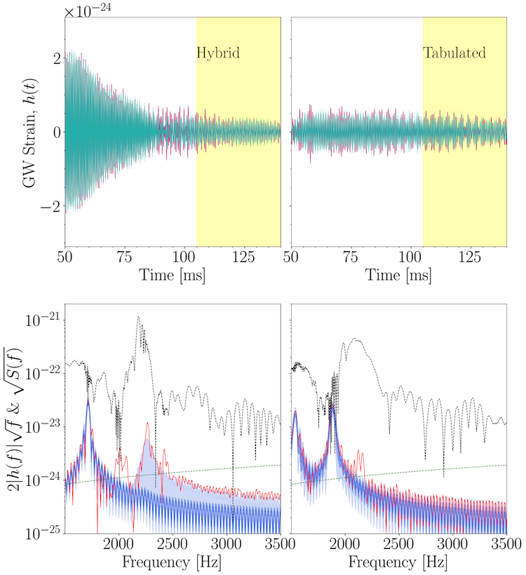
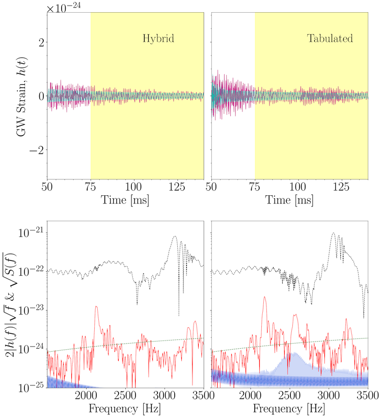
Figure 8: Waveforms (top row) and ASD (bottom row) of the injected (red) and reconstructed (blue) late post-merger GW signals for a source located at $D=7$ Mpc. The left panel corresponds to the HShen EoS and the right panel to the SLy4 EoS. Within each panel, the left (right) column displays the hybrid (tabulated) version of the respective EoS. The black and green dotted lines in the bottom-row plots are the ASD computed from the complete waveforms and the sensitivity curve of the ET detector, respectively.

IV.1.4 Tidal deformability

The frequency peaks of the early post-merger phase of the remnant can be used to infer properties of neutron stars by exploiting correlations with physical parameters through EoS-insensitive, quasi-universal relations (see e.g. Read et al. (2013); Bernuzzi et al. (2014); Bauswein and Stergioulas (2015); Takami et al. (2015); Rezzolla and Takami (2016); Bauswein and Stergioulas (2019); Bauswein et al. (2019); Soultanis et al. (2022); Topolski et al. (2023)). In particular, a number of empirical fits between the frequencies of various modes (e.g. the peak frequency at merger, the $f_{2,i}$ mode, and the $f_{2}$ mode) and the tidal deformability parameter $\Lambda$ characterising the quadrupole deformability of an isolated neutron star, have been proposed (see Soultanis et al. (2022); Topolski et al. (2023) and references therein for up-to-date revisions of existing literature). In Guerra et al. (2024) we present new fits of the frequencies of the $f_{2,i}$ and $f_{2}$ modes to the tidal deformability parameter using our set of EoS. We note that those quasi-universal relations are built using hybrid EoS only since the number of simulations with tabulated EoS is not large enough to yield a meaningful fit. However, their validity when applied to simulations with tabulated EoS can be tested, using the standard deviation of the correlation for the hybrid EoS as a reference metric. For the $f_{2,i}$ and $f_{2}$ modes, the standard deviation is $67.54$ Hz and $97.56$ Hz, respectively Guerra et al. (2024). Using those fits we discuss here the posterior probability distributions of the tidal deformability parameter obtained from both, the frequencies of the $f_{2,i}$ and $f_{2}$ modes, and for the two different treatments of thermal effects.

In the top row of Figure 7 we show the results for the $f_{2,i}$ mode, for different distances and all four EoS. The distributions displayed are built using the empirical relations from Guerra et al. (2024). The upper panels correspond to the hybrid version of the EoS and the lower panels to the tabulated version. Since $\Lambda_{i}$ is directly calculated from $f_{2,i}$, the behaviour of the posterior distributions of the two quantities with the distance is the same (cf. uppermost row of Fig. 5). Our results indicate that $\Lambda_{i}$ could be reconstructed up to $D\approx 200$ Mpc for all EoS except for SLy4 for which the reconstruction is acceptable only up to $D\lesssim 100$ Mpc. For the SLy4 EoS (first column), the distributions of $\Lambda_{i}$ are closer to the injected value (red vertical dashed line) for the tabulated version. On the other hand, HShen and DD2 both yield a good recovery of $\Lambda_{i}$ for all the distances shown. Their $p$-values at 200 Mpc are above 0.175 for both versions of the EoS.

The tidal deformability parameter can also be computed using the frequency of the $f_{2}$ mode. To do so we use the fits for this mode presented in Guerra et al. (2024). The LS220 EoS is discarded in this analysis because at the post-merger times considered the evolution of the remnant when using the hybrid version of this EoS already shows the formation of a BH. The differences on the distributions of $\Lambda$ between the hybrid and tabulated versions of the EoS for the $f_{2}$ mode are displayed in the bottom row of Fig. 7. As expected, the posterior distributions are similar to those obtained with the $f_{2}$ mode (middle row of Fig. 5). The most stricking difference is that for the tabulated version of the HShen EoS, $\Lambda$ is inaccurately inferred at $D=200$ Mpc.

As stated in Section II using tabulated or hybrid EoS leads to slightly different initial neutron star configurations and, thus, to different values of the tidal deformability. This is why the vertical black lines displayed in Fig. 7, corresponding to the values of $\Lambda$ reported in Table 1, are not the same for the two approaches for the EoS. This figure shows that the empirical fits of Guerra et al. (2024) can be also applied to simulations with tabulated EoS in most cases, as the variations in frequency are within one standard deviation of the mean of the correlation. In general, we find that the fit for the $f_{2,i}$ mode (red vertical lines) is closest to the “true” value from the simulation. We observe that the tidal deformability might be detected up to several tens of Mpc for all EoS (when computed from empirical fits built for hybrid models only).

IV.2 Late post-merger phase: inertial modes

At later post-merger times than those considered in the preceding section ($t\gtrsim 50$ ms) the amplitude of the $f_{2}$ mode decreases and convective instabilities in the interior of the remnant set in (see De Pietri et al. (2018, 2020); Guerra et al. (2024)). Those trigger the excitation of inertial modes whose dynamics leave an imprint in the late post-merger signal. Inertial modes attain smaller amplitudes than the modes from the early post-merger phase and their frequency peaks in the spectra are also lower than those of the $f_{2,i}$ and $f_{2}$ modes.

IV.2.1 Waveform reconstructions

Figure 8 shows the non-whitened, time-domain signal (top row) and the ASD (bottom row) of the injected (red) and reconstructed (blue) late post-merger GW signals (with the detector ASD), for a source located at a distance of 7 Mpc. The left panel shows the waveforms and ASD for the HShen EoS while the right panel displays the corresponding quantities for the case of the SLy4 EoS. Within each panel, the left (right) column correspond to the hybrid (tabulated) version of the respective EoS. As before, the ASD shown in the bottom row have been computed by Fourier-transforming the waveforms in the time windows highlighted in yellow in the plots in the top row (see also Table 2). Likewise, the blue-shaded regions in the ASD plots in both figures show the 50% and 90% CI of the distribution of the reconstructed waveforms.

At the distance considered and regardless of the treatment of thermal effects, the reconstructions of the late-time signals BayesWave produces are only accurate for the HShen EoS. This is due to the small amplitude of the late post-merger signal in the case of SLy4. The frequency peak of the dominant inertial mode for this EoS is located around 2.2 kHz (see the ASD of the injected signal, colored in red). Despite the peak amplitude is above the sensitivity curve of the ET detector, BayesWave cannot correctly capture it, as apparent from the CI of the reconstructed distributions. Regarding the HShen EoS, the dominant frequency peak of the inertial modes is located below 2 kHz for both versions of the EoS. In the case of the tabulated version two peaks are visible around 1.5 kHz and 2 kHz, while for the hybrid version of this EoS those two peaks appear at frequencies around 1.75 kHz and 2.5 kHz. Notice that the peak located at around 2 kHz for the tabulated EoS is actually the $f_{2}$ mode. This mode is not yet completely damped at this late post-merger time. Therefore, we do not consider it when computing the posterior probability for the frequency peaks in the last row of Fig. 5. The same explanation holds for the peak at around 2.5 kHz in the hybrid case (see Guerra et al. (2024) for more details).

IV.2.2 Frequency peaks of the inertial modes

The posterior distributions of the frequency peaks of the inertial modes are displayed in the bottom row of Fig. 5 for all EoS except LS220 (as the simulation with the hybrid version of this EoS collapses to a BH at early post-merger times). The upper (lower) rows in this figure represent the hybrid (tabulated) versions of the corresponding EoS. The injections, whose frequencies are depicted by the dashed vertical lines, are now performed at much shorter distances than we did for the $f_{2,i}$ and $f_{2}$ modes, due to the smaller amplitude of inertial modes. The largest distance considered is now $D=15$ Mpc.

The characteristic peak frequencies of inertial modes, $f_{\rm inertial}$, are lower than the ones from the fundamental modes, $f_{2,i}$ and $f_{2}$, as can be seen by direct comparison in Fig. 5. As for the quadrupolar modes, inertial modes also display a shift in frequencies depending on the particular treatment of thermal effects in the EoS. This shift appears to be only detectable for the case of the HShen EoS (middle panel) as the posterior distributions of the hybrid and the tabulated versions of the EoS do not overlap up to $D\approx 10$ Mpc. On the other hand, the small amplitude of the late post-merger signal for the SLy4 EoS is too low to yield a good reconstruction unless the source is located at a distance of less than 5 Mpc. Only for such short distances the frequency shift in the posterior distributions might be distinguished.

IV.2.3 Overlap of the inertial modes

As we did before for the $f_{2,i}$ and $f_{2}$ modes, we also use the network overlap function to assess the reconstruction of the waveforms for the case of inertial modes. Those overlaps are shown in the bottom row of Figure 6. For the SLy4 EoS (first column) the overlap is above 0.5 for a distance to the source of less than 5 Mpc, with the tabulated version of the EoS attaining a higher value of the overlap for slightly larger distances. For both implementations of the thermal effects, the average overlap falls below 0.25 for distances above $\approx 7$ Mpc, which means that the injected and reconstructed waveforms differ considerably. Correspondingly, the waveform signals for HShen and DD2 (second and third columns, respectively) are still reconstructed with a network overlap over 0.5 up to a distance of about 12 Mpc. The tabulaled version of the HShen EoS is more poorly recovered than its hybrid counterpart, with a smaller overlap at about 10 Mpc. Finally, in the case of the LS220 EoS (fourth column), the network overlap is above 0.5 for distances up to 15 Mpc. Notice that only the overlap of the tabulated version of LS220 is plotted in Fig. 6 as the simulation with a hybrid EoS collapses to a BH before inertial modes have been excited.

V Conclusions

Numerical simulations of BNS mergers incorporate thermal effects in the EoS using two alternative approaches. The first one is a hybrid approach which assumes that the pressure and the internal energy are composed of two constituents, a cold, zero temperature part described by a family of piecewise polytropes and a thermal part described by an ideal-gas-like EoS. The second approach employs tabulated representations of microphysical finite-temperature EoS, providing a self-consistent method to probe the impact of thermal effects in the merger dynamics. These two ways of incorporating thermal effects in the numerical modelling lead to measurable differences in the GW signal, especially in the post-merger emission, well visible in the frequency spectra (see e.g. Bauswein et al. (2010); Guerra et al. (2024)). In this paper we have investigated the prospects for identifying such differences by reconstructing the GW signals of Guerra et al. (2024) using BayesWave Cornish and Littenberg (2015); Littenberg and Cornish (2015), building on our previous work in Miravet-Tenés et al. (2023) where we focused on inertial modes only, excited in the very late part of the post-merger signal. Here, we have considered the entire post-merger signal, i.e. both its early part where the fundamental quadrupolar $f_{2}$ mode dominates the GW spectrum and its late part where inertial modes are excited. The time-domain waveforms of Guerra et al. (2024), obtained through BNS merger simulations with four different EoS, accounting for both descriptions of thermal effects, have been injected into Gaussian noise given by the sensitivity of the third-generation detector Einstein Telescope Punturo et al. (2010); Hild et al. (2011), selecting optimal sky location and inclination. (Results for non-optimal configurations are discussed in Appendix A.) The capability of BayesWave to reconstruct the injected signals has been assessed by computing the overlap function of the detector network. As the post-merger remnant evolves the amplitude of the GW signal significantly decreases, resulting in a corresponding reduction of the overlap between injected and reconstructed waveforms. The same occurs as the distance to the source increases, irrespective of the portion of the post-merger signal being analyzed.

The two representations of thermal effects in the EoS result in frequency shifts of the dominant peaks in the GW spectra. In some cases, those differences are large enough to be told apart, especially in the early post-merger phase, when the signal amplitude is the loudest, and at sufficiently small distances. The detectability prospects have been found to strongly depend on the EoS. Both, the SLy4 EoS (at small enough distances) and the HShen EoS (at significantly bigger distances) present large frequency shifts of the dominant $f_{2,i}$ and $f_{2}$ modes. These shifts may allow to distinguish the differences in the implementation of thermal effects between hybrid and tabulated versions of these two EoS with third-generation detectors. On the other hand, for the DD2 and LS220 EoS, no large enough frequency shifts between the hybrid and tabulated cases have been found to unambiguously differentiate with BayesWave the treatment of thermal effects in the EoS.

Differences in the dominant peaks of the GW spectra are still present during the late post-merger phase, where the inertial modes dominate Kastaun (2008); De Pietri et al. (2018, 2020); Guerra et al. (2024). These modes are associated with a part of the GW signal with a much lower amplitude than that of the $f_{2,i}$ and $f_{2}$ modes. Therefore, they are more difficult to detect Miravet-Tenés et al. (2023). Our results indicate that third-generation detectors such as ET may be able to observe inertial modes up to a distance of about 10 Mpc, depending of the EoS. For this late-time part of the signal, the shift in the peak frequency due to the different treatment of thermal effects can be above 200 Hz at most, for the case of the HShen EoS. On the other hand, for the LS220 EoS, the difference is more obvious: the hybrid version of this EoS leads to the collapse of the remnant to a black hole, as opposed to the tabulated version of the same EoS Guerra et al. (2024).

Finally, we have also computed the tidal deformability from the frequency peaks of both the $f_{2,i}$ and $f_{2}$ modes and through the empirical fits presented in Guerra et al. (2024). The differences in thermal effects between the hybrid and the tabulated EoS inferred through the analysis of the tidal deformability parameter are also more apparent for the $f_{2}$ mode, since the shift in the frequency peaks is more pronounced.

The results of the work reported here are consistent with those recently presented by Villa-Ortega et al. (2023) who employed Bayesian model selection to explore differences between the hybrid and the tabulated approaches for the same set of GW signals. The differences in the posterior distributions of the main frequency peaks in the early post-merger GW spectra in hybrid and tabulated models reported here might be resolved in third-generation detectors up to distances of about tens of Mpc, compatible with the values found by Villa-Ortega et al. (2023).

Appendix A Reconstruction of injections with non-optimal sky location and orientation

The injections discussed in the main text of this paper were performed considering an optimal source inclination with respect to the ET detector $(\iota=0)$ and an optimal sky location, with a right ascension of 2.9109 rad and a declination of 0.7627 rad. Therefore, the results represent the best-case scenario for a given source distance. However, in reality the source can be anywhere in the sky and have an arbitrary declination. Hence, the effective distance to the source can be actually larger. This possibility is briefly discussed in this appendix.

In Table 3 we report the value of the overlap function for the fundamental quadrupolar frequency peaks for a source at a distance $D=150$ Mpc and for different combinations of sky locations and inclinations. We only consider the hybrid version of the HShen EoS as this is the one yielding the best detectability prospects in the optimal case. The non-optimal inclination is set to $\iota=0.5585$ rad and the right ascension and declination in the sky for a representative non-optimal case are chosen to be 3.4462 rad and 0.45 rad, respectively. As expected, the overlap function decreases with respect to the optimal case. The lowest values found are $78.5\%$ (with respect to the optimal case) and $87.2\%$ for the $f_{2,i}$ and $f_{2}$ modes, respectively. Therefore, for signals coming from a non-optimal sky location and/or from a source with a non-optimal inclination, the effective distance will not be much larger than the optimal case. Furthermore, we note that the effect of the actual sky position of the source will become less of a concern if a network of detectors built in different locations is used.

Table 3: Overlap functions for different inclinations and sky locations for a distance $D=150$ Mpc to the source. The first (second) row corresponds to the mode $f_{2,i}$ ($f_{2}$). In parenthesis we show the percentage value with respect to the overlap for the optimal case.

Mode	Optimal $\iota$	Non-optimal $\iota$	Optimal $\iota$	Non-optimal $\iota$
	Optimal	Optimal	Non-optimal	Non-optimal
	sky loc	sky loc	sky loc	sky loc
$f_{2,i}$	0.803	0.650 (81.0 %)	0.656 (81.7 %)	0.630 (78.5 %)
$f_{2}$	0.835	0.791 (94.7 %)	0.793 (95.0 %)	0.728 (87.2 %)

References

- Abbott et al. (2019a) B. P. Abbott, R. Abbott, T. D. Abbott, S. Abraham, F. Acernese, K. Ackley, C. Adams, R. X. Adhikari, V. B. Adya, C. Affeldt, et al., Physical Review X 9, 031040 (2019a), eprint 1811.12907.
- Abbott et al. (2021) R. Abbott, T. D. Abbott, S. Abraham, F. Acernese, K. Ackley, A. Adams, C. Adams, R. X. Adhikari, V. B. Adya, C. Affeldt, et al., Physical Review X 11, 021053 (2021), eprint 2010.14527.
- The LIGO Scientific Collaboration et al. (2021) The LIGO Scientific Collaboration, the Virgo Collaboration, R. Abbott, T. D. Abbott, F. Acernese, K. Ackley, C. Adams, N. Adhikari, R. X. Adhikari, V. B. Adya, et al., arXiv e-prints arXiv:2108.01045 (2021), eprint 2108.01045.
- Abbott et al. (2023) R. Abbott, T. D. Abbott, F. Acernese, K. Ackley, C. Adams, N. Adhikari, R. X. Adhikari, V. B. Adya, C. Affeldt, D. Agarwal, et al., Physical Review X 13, 011048 (2023), eprint 2111.03634.
- Abbott et al. (2017a) B. P. Abbott et al. (LIGO Scientific, Virgo), Astrophys. J. Lett. 850, L39 (2017a), eprint 1710.05836.
- Abbott et al. (2017b) B. P. Abbott et al. (LIGO Scientific, Virgo, Fermi GBM, INTEGRAL, IceCube, AstroSat Cadmium Zinc Telluride Imager Team, IPN, Insight-Hxmt, ANTARES, Swift, AGILE Team, 1M2H Team, Dark Energy Camera GW-EM, DES, DLT40, GRAWITA, Fermi-LAT, ATCA, ASKAP, Las Cumbres Observatory Group, OzGrav, DWF (Deeper Wider Faster Program), AST3, CAASTRO, VINROUGE, MASTER, J-GEM, GROWTH, JAGWAR, CaltechNRAO, TTU-NRAO, NuSTAR, Pan-STARRS, MAXI Team, TZAC Consortium, KU, Nordic Optical Telescope, ePESSTO, GROND, Texas Tech University, SALT Group, TOROS, BOOTES, MWA, CALET, IKI-GW Follow-up, H.E.S.S., LOFAR, LWA, HAWC, Pierre Auger, ALMA, Euro VLBI Team, Pi of Sky, Chandra Team at McGill University, DFN, ATLAS Telescopes, High Time Resolution Universe Survey, RIMAS, RATIR, SKA South Africa/MeerKAT), Astrophys. J. 848, L12 (2017b), eprint 1710.05833.
- Abbott et al. (2017c) B. P. Abbott et al. (LIGO Scientific, Virgo, Fermi-GBM, INTEGRAL), Astrophys. J. Lett. 848, L13 (2017c), eprint 1710.05834.
- Li and Paczynski (1998) L.-X. Li and B. Paczynski, Astrophys. J. Lett. 507, L59 (1998), eprint astro-ph/9807272.
- Metzger (2017) B. D. Metzger, Living Rev. Rel. 20, 3 (2017), eprint 1610.09381.
- Troja et al. (2017) E. Troja, L. Piro, H. van Eerten, R. T. Wollaeger, M. Im, O. D. Fox, N. R. Butler, S. B. Cenko, T. Sakamoto, C. L. Fryer, et al., Nature (London) 551, 71 (2017), eprint 1710.05433.
- Kasen et al. (2017) D. Kasen, B. Metzger, J. Barnes, E. Quataert, and E. Ramirez-Ruiz, Nature (London) 551, 80 (2017), eprint 1710.05463.
- Abbott et al. (2017a) B. P. Abbott, R. Abbott, T. D. Abbott, F. Acernese, K. Ackley, C. Adams, T. Adams, P. Addesso, R. X. Adhikari, V. B. Adya, et al., Nature (London) 551, 85 (2017a), eprint 1710.05835.
- Dietrich et al. (2020) T. Dietrich, M. W. Coughlin, P. T. H. Pang, M. Bulla, J. Heinzel, L. Issa, I. Tews, and S. Antier, Science 370, 1450 (2020), eprint 2002.11355.
- Rezzolla et al. (2018) L. Rezzolla, E. R. Most, and L. R. Weih, Astrophys. J. Lett. 852, L25 (2018), eprint 1711.00314.
- Ruiz et al. (2018) M. Ruiz, S. L. Shapiro, and A. Tsokaros, Phys. Rev. D 97, 021501 (2018), eprint 1711.00473.
- Shibata et al. (2017) M. Shibata, S. Fujibayashi, K. Hotokezaka, K. Kiuchi, K. Kyutoku, Y. Sekiguchi, and M. Tanaka, Phys. Rev. D 96, 123012 (2017), eprint 1710.07579.
- Margalit and Metzger (2017) B. Margalit and B. D. Metzger, Astrophys. J. Lett. 850, L19 (2017), eprint 1710.05938.
- Abbott et al. (2018) B. P. Abbott, R. Abbott, T. D. Abbott, F. Acernese, K. Ackley, C. Adams, T. Adams, P. Addesso, R. X. Adhikari, V. B. Adya, et al., Phys. Rev. Lett. 121, 161101 (2018), eprint 1805.11581.
- Abbott et al. (2019b) B. P. Abbott, R. Abbott, T. D. Abbott, F. Acernese, K. Ackley, C. Adams, T. Adams, P. Addesso, R. X. Adhikari, V. B. Adya, et al., Physical Review X 9, 011001 (2019b), eprint 1805.11579.
- Abbott et al. (2017b) B. P. Abbott, R. Abbott, T. D. Abbott, F. Acernese, K. Ackley, C. Adams, T. Adams, P. Addesso, R. X. Adhikari, V. B. Adya, et al., ApJL 851, L16 (2017b), eprint 1710.09320.
- Lackey et al. (2017) B. D. Lackey, S. Bernuzzi, C. R. Galley, J. Meidam, and C. Van Den Broeck, Phys. Rev. D 95, 104036 (2017), eprint 1610.04742.
- Narikawa and Uchikata (2022) T. Narikawa and N. Uchikata, Phys. Rev. D 106, 103006 (2022), eprint 2205.06023.
- Sun et al. (2022) L. Sun, M. Ruiz, S. L. Shapiro, and A. Tsokaros, Phys. Rev. D 105, 104028 (2022), eprint 2202.12901.
- Foucart et al. (2023) F. Foucart, M. D. Duez, R. Haas, L. E. Kidder, H. P. Pfeiffer, M. A. Scheel, and E. Spira-Savett, Phys. Rev. D 107, 103055 (2023), eprint 2210.05670.
- Foucart et al. (2020) F. Foucart, M. D. Duez, F. Hebert, L. E. Kidder, H. P. Pfeiffer, and M. A. Scheel, Astrophys. J. Lett. 902, L27 (2020), eprint 2008.08089.
- Gieg et al. (2022) H. Gieg, F. Schianchi, T. Dietrich, and M. Ujevic, Universe 8, 370 (2022), eprint 2206.01337.
- Hayashi et al. (2022) K. Hayashi, S. Fujibayashi, K. Kiuchi, K. Kyutoku, Y. Sekiguchi, and M. Shibata, Phys. Rev. D 106, 023008 (2022), eprint 2111.04621.
- Radice et al. (2022) D. Radice, S. Bernuzzi, A. Perego, and R. Haas, Mon. Not. Roy. Astron. Soc. 512, 1499 (2022), eprint 2111.14858.
- Janka et al. (1993) H. T. Janka, T. Zwerger, and R. Moenchmeyer, ”Astronomy and Astrophysics” 268, 360 (1993).
- Dimmelmeier et al. (2002) H. Dimmelmeier, J. A. Font, and E. Muller, Astron. Astrophys. 388, 917 (2002), eprint astro-ph/0204288.
- Shibata et al. (2005) M. Shibata, K. Taniguchi, and K. Uryu, Phys. Rev. D 71, 084021 (2005), eprint gr-qc/0503119.
- Constantinou et al. (2015) C. Constantinou, B. Muccioli, M. Prakash, and J. M. Lattimer, Phys. Rev. C 92, 025801 (2015), eprint 1504.03982.
- Takami et al. (2015) K. Takami, L. Rezzolla, and L. Baiotti, Phys. Rev. D 91, 064001 (2015), eprint 1412.3240.
- Lim and Holt (2019) Y. Lim and J. W. Holt (2019), eprint 1909.09089.
- Raithel et al. (2021) C. Raithel, V. Paschalidis, and F. Özel, Phys. Rev. D 104, 063016 (2021), eprint 2104.07226.
- Bauswein et al. (2010) A. Bauswein, H. T. Janka, and R. Oechslin, Phys. Rev. D 82, 084043 (2010), eprint 1006.3315.
- Figura et al. (2021) A. Figura, F. Li, J.-J. Lu, G. F. Burgio, Z.-H. Li, and H. J. Schulze, Phys. Rev. D 103, 083012 (2021), eprint 2103.02365.
- Oechslin et al. (2007) R. Oechslin, H. T. Janka, and A. Marek, Astron. Astrophys. 467, 395 (2007), eprint astro-ph/0611047.
- Sekiguchi et al. (2011) Y. Sekiguchi, K. Kiuchi, K. Kyutoku, and M. Shibata, Phys. Rev. Lett. 107, 051102 (2011), eprint 1105.2125.
- Fields et al. (2023) J. Fields, A. Prakash, M. Breschi, D. Radice, S. Bernuzzi, and A. d. S. Schneider (2023), eprint 2302.11359.
- Espino et al. (2022) P. L. Espino, G. Bozzola, and V. Paschalidis (2022), eprint 2210.13481.
- Werneck et al. (2023) L. R. Werneck et al., Phys. Rev. D 107, 044037 (2023), eprint 2208.14487.
- Guerra et al. (2024) D. Guerra, M. Ruiz, M. Pasquali, P. Cerdá-Duran, J. A. Font, and A. Rios, in preparation (2024).
- Stergioulas et al. (2011) N. Stergioulas, A. Bauswein, K. Zagkouris, and H.-T. Janka, Mon. Not. Roy. Astron. Soc. 418, 427 (2011), eprint 1105.0368.
- Hotokezaka et al. (2013) K. Hotokezaka, K. Kiuchi, K. Kyutoku, T. Muranushi, Y.-i. Sekiguchi, M. Shibata, and K. Taniguchi, Phys. Rev. D 88, 044026 (2013), eprint 1307.5888.
- Bauswein and Stergioulas (2015) A. Bauswein and N. Stergioulas, Phys. Rev. D 91, 124056 (2015), eprint 1502.03176.
- Takami et al. (2015) K. Takami, L. Rezzolla, and L. Baiotti, Phys. Rev. D 91, 064001 (2015), eprint 1412.3240.
- Bauswein et al. (2016) A. Bauswein, N. Stergioulas, and H.-T. Janka, European Physical Journal A 52, 56 (2016), eprint 1508.05493.
- Bauswein and Stergioulas (2019) A. Bauswein and N. Stergioulas, Journal of Physics G Nuclear Physics 46, 113002 (2019), eprint 1901.06969.
- Rezzolla and Takami (2016) L. Rezzolla and K. Takami, Phys. Rev. D 93, 124051 (2016), eprint 1604.00246.
- Read et al. (2013) J. S. Read, L. Baiotti, J. D. E. Creighton, J. L. Friedman, B. Giacomazzo, K. Kyutoku, C. Markakis, L. Rezzolla, M. Shibata, and K. Taniguchi, Phys. Rev. D 88, 044042 (2013), eprint 1306.4065.
- Topolski et al. (2023) K. Topolski, S. Tootle, and L. Rezzolla (2023), eprint 2310.10728.
- De Pietri et al. (2018) R. De Pietri, A. Feo, J. A. Font, F. Löffler, F. Maione, M. Pasquali, and N. Stergioulas, Phys. Rev. Lett. 120, 221101 (2018), eprint 1802.03288.
- De Pietri et al. (2020) R. De Pietri, A. Feo, J. A. Font, F. Löffler, M. Pasquali, and N. Stergioulas, Phys. Rev. D 101, 064052 (2020), eprint 1910.04036.
- Kastaun (2008) W. Kastaun, Phys. Rev. D 77, 124019 (2008), eprint 0804.1151.
- Cornish and Littenberg (2015) N. J. Cornish and T. B. Littenberg, Classical and Quantum Gravity 32, 135012 (2015), eprint 1410.3835.
- Littenberg and Cornish (2015) T. B. Littenberg and N. J. Cornish, Phys. Rev. D 91, 084034 (2015), eprint 1410.3852.
- Miravet-Tenés et al. (2023) M. Miravet-Tenés, F. L. Castillo, R. De Pietri, P. Cerdá-Durán, and J. A. Font, Phys. Rev. D 107, 103053 (2023), eprint 2302.04553.
- Punturo et al. (2010) M. Punturo, M. Abernathy, F. Acernese, B. Allen, N. Andersson, K. Arun, F. Barone, B. Barr, M. Barsuglia, M. Beker, et al., Classical and Quantum Gravity 27, 194002 (2010).
- Hild et al. (2011) S. Hild, M. Abernathy, F. Acernese, P. Amaro-Seoane, N. Andersson, K. Arun, F. Barone, B. Barr, M. Barsuglia, M. Beker, et al., Classical and Quantum Gravity 28, 094013 (2011), eprint 1012.0908.
- Maggiore et al. (2020) M. Maggiore, C. Van Den Broeck, N. Bartolo, E. Belgacem, D. Bertacca, M. A. Bizouard, M. Branchesi, S. Clesse, S. Foffa, J. García-Bellido, et al., JCAP 2020, 050 (2020), eprint 1912.02622.
- Branchesi et al. (2023) M. Branchesi, M. Maggiore, D. Alonso, C. Badger, B. Banerjee, F. Beirnaert, E. Belgacem, S. Bhagwat, G. Boileau, S. Borhanian, et al., JCAP 2023, 068 (2023), eprint 2303.15923.
- Villa-Ortega et al. (2023) V. Villa-Ortega, A. Lorenzo-Medina, J. Calderón Bustillo, M. Ruiz, D. Guerra, P. Cerdá-Duran, and J. A. Font, arXiv e-prints arXiv:2310.20378 (2023), eprint 2310.20378.
- Raithel and Paschalidis (2023) C. A. Raithel and V. Paschalidis, arXiv e-prints arXiv:2312.14046 (2023), eprint 2312.14046.
- Typel et al. (2010) S. Typel, G. Ropke, T. Klahn, D. Blaschke, and H. H. Wolter, Phys. Rev. C 81, 015803 (2010), eprint 0908.2344.
- Shen et al. (2011) H. Shen, H. Toki, K. Oyamatsu, and K. Sumiyoshi, Astrophys. J. Suppl. 197, 20 (2011), eprint 1105.1666.
- James M. Lattimer (1991) F. D. S. James M. Lattimer, Nucl. Phys. A 535, 331 (1991).
- Chabanat et al. (1998) E. Chabanat, P. Bonche, P. Haensel, J. Meyer, and R. Shaeffer, Nucl. Phys. A 635, 231 (1998).
- Gourgoulhon et al. (2001) E. Gourgoulhon, P. Grandclement, K. Taniguchi, J.-A. Marck, and S. Bonazzola, Phys. Rev. D 63, 064029 (2001), eprint gr-qc/0007028.
- Taniguchi and Gourgoulhon (2002) K. Taniguchi and E. Gourgoulhon, Phys. Rev. D 66, 104019 (2002).
- (71) http://www.lorene.obspm.fr/.
- Schneider et al. (2017) A. S. Schneider, L. F. Roberts, and C. D. Ott, Phys. Rev. C 96, 065802 (2017), eprint 1707.01527.
- (73) https://stellarcollapse.org/SROEOS.
- Pilgrim (2021) C. Pilgrim, The Journal of Open Source Software 6, 3859 (2021).
- Read et al. (2009) J. S. Read, B. D. Lackey, B. J. Owen, and J. L. Friedman, Phys. Rev. D79, 124032 (2009).
- Etienne et al. (2015) Z. B. Etienne, V. Paschalidis, R. Haas, P. Mösta, and S. L. Shapiro, Class. Quant. Grav. 32, 175009 (2015), eprint 1501.07276.
- Loffler et al. (2012) F. Loffler et al., Class. Quant. Grav. 29, 115001 (2012), eprint 1111.3344.
- Noble et al. (2006) S. C. Noble, C. F. Gammie, J. C. McKinney, and L. Del Zanna, Astrophys. J. 641, 626 (2006), eprint astro-ph/0512420.
- Baumgarte and Shapiro (1998) T. W. Baumgarte and S. L. Shapiro, Phys. Rev. D 59, 024007 (1998), eprint gr-qc/9810065.
- Shibata and Nakamura (1995) M. Shibata and T. Nakamura, Phys. Rev. D 52, 5428 (1995), URL http://link.aps.org/doi/10.1103/PhysRevD.52.5428.
- Banyuls et al. (1997) F. Banyuls, J. A. Font, J. M. Ibáñez, J. M. Martí, and J. A. Miralles, Astrophys. J. 476, 221 (1997).
- Font (2008) J. A. Font, Living Reviews in Relativity 11, 7 (2008).
- Bécsy et al. (2017) B. Bécsy, P. Raffai, N. J. Cornish, R. Essick, J. Kanner, E. Katsavounidis, T. B. Littenberg, M. Millhouse, and S. Vitale, Astrophys. J. 839, 15 (2017), eprint 1612.02003.
- Cooley and Tukey (1965) J. W. Cooley and J. W. Tukey, Mathematics of Computation 19, 297 (1965).
- Kastaun (2021) W. Kastaun, PyCactus: Post-processing tools for Cactus computational toolkit simulation data, Astrophysics Source Code Library, record ascl:2107.017 (2021), eprint 2107.017.
- Chatziioannou et al. (2017) K. Chatziioannou, J. A. Clark, A. Bauswein, M. Millhouse, T. B. Littenberg, and N. Cornish, Phys. Rev. D 96, 124035 (2017).
- Evans et al. (2021) M. Evans, R. X. Adhikari, C. Afle, S. W. Ballmer, S. Biscoveanu, S. Borhanian, D. A. Brown, Y. Chen, R. Eisenstein, A. Gruson, et al., arXiv e-prints arXiv:2109.09882 (2021), eprint 2109.09882.
- Blackburn et al. (2008) L. Blackburn, L. Cadonati, S. Caride, S. Caudill, S. Chatterji, N. Christensen, J. Dalrymple, S. Desai, A. Di Credico, G. Ely, et al., Classical and Quantum Gravity 25, 184004 (2008), eprint 0804.0800.
- Abbott et al. (2009) B. P. Abbott, R. Abbott, R. Adhikari, P. Ajith, B. Allen, G. Allen, R. S. Amin, S. B. Anderson, W. G. Anderson, M. A. Arain, et al., Reports on Progress in Physics 72, 076901 (2009), eprint 0711.3041.
- Aasi et al. (2012) J. Aasi, J. Abadie, B. P. Abbott, R. Abbott, T. D. Abbott, M. Abernathy, T. Accadia, F. Acernese, C. Adams, T. Adams, et al., Classical and Quantum Gravity 29, 155002 (2012), eprint 1203.5613.
- Bernuzzi et al. (2014) S. Bernuzzi, A. Nagar, S. Balmelli, T. Dietrich, and M. Ujevic, Phys. Rev. Lett. 112, 201101 (2014), eprint 1402.6244.
- Bauswein et al. (2019) A. Bauswein, N.-U. F. Bastian, D. B. Blaschke, K. Chatziioannou, J. A. Clark, T. Fischer, and M. Oertel, Phys. Rev. Lett. 122, 061102 (2019), eprint 1809.01116.
- Soultanis et al. (2022) T. Soultanis, A. Bauswein, and N. Stergioulas, Phys. Rev. D 105, 043020 (2022), eprint 2111.08353.
- Topolski et al. (2023) K. Topolski, S. Tootle, and L. Rezzolla, arXiv e-prints arXiv:2310.10728 (2023), eprint 2310.10728.
- Harris et al. (2020) C. R. Harris, K. J. Millman, S. J. van der Walt, R. Gommers, P. Virtanen, D. Cournapeau, E. Wieser, J. Taylor, S. Berg, N. J. Smith, et al., Nature 585, 357 (2020), URL https://doi.org/10.1038/s41586-020-2649-2.
- Virtanen et al. (2020) P. Virtanen, R. Gommers, T. E. Oliphant, M. Haberland, T. Reddy, D. Cournapeau, E. Burovski, P. Peterson, W. Weckesser, J. Bright, et al., Nature Methods 17, 261 (2020).
- Pedregosa et al. (2011) F. Pedregosa, G. Varoquaux, A. Gramfort, V. Michel, B. Thirion, O. Grisel, M. Blondel, P. Prettenhofer, R. Weiss, V. Dubourg, et al., Journal of Machine Learning Research 12, 2825 (2011).
- Hunter (2007) J. D. Hunter, Computing in Science & Engineering 9, 90 (2007).