Parameter Space of Leptogenesis in Polynomial Inflation

Abstract

Polynomial inflation is a very simple and well motivated scenario. A potential with a concave “almost” saddle point at field value $\phi=\phi_{0}$ fits well the cosmic microwave background (CMB) data and makes testable predictions for the running of the spectral index and the tensor to scalar ratio. In this work we analyze leptogenesis in the polynomial inflation framework. We delineate the allowed parameter space giving rise to the correct baryon asymmetry as well as being consistent with data on neutrino oscillations. To that end we consider two different reheating scenarios. $(i)$ If the inflaton decays into two bosons, the reheating temperature can be as high as $T_{\text{rh}}\sim 10^{14}$ GeV without spoiling the flatness of the potential, allowing vanilla $N_{1}$ thermal leptogenesis to work if $T_{\text{rh}}>M_{1}$ where $N_{1}$ is the lightest right–handed neutrino and $M_{1}$ its mass. Moreover, if the dominant decay of the inflaton is into Higgs bosons of the Standard Model, we find that rare three–body inflaton decays into a Higgs boson plus one light and one heavy neutrino allow leptogenesis even for $T_{\text{rh}}<M_{1}$ if the inflaton mass is of order $10^{12}$ GeV or higher; in the polynomial inflation scenario this requires $\phi_{0}\gtrsim 2.5~{}M_{P}$. This novel mechanism of non–thermal leptogenesis is quite generic, since the coupling leading to the three–body final state is required in the type I see–saw mechanism. $(ii)$ If the inflaton decays into two fermions, the flatness of the potential implies a lower reheating temperature. In this case inflaton decay to two $N_{1}$ still allows successful non–thermal leptogenesis if $\phi_{0}\gtrsim 0.1~{}M_{P}$ and $T_{\text{rh}}\gtrsim 10^{6}$ GeV.

1 Introduction

Monomial inflationary scenarios have been ruled out by recent Planck and BICEP/Keck 2018 measurements Planck:2018jri ; BICEP:2021xfz . We have recently shown that a simple polynomial of degree four with a concave “almost” saddle point at field value $\phi=\phi_{0}$ can nevertheless fit well the CMB data Drees:2021wgd ; Drees:2022aea . The model predicts the running of the spectral index to be $\mathcal{O}(10^{-3})$, which may be testable by the next generation of cosmic microwave background (CMB) experiments in combination with data on structure formation at smaller scales Munoz:2016owz . The predicted tensor to scalar ratio $r$ (in the large field scenario) can saturate the current bound.

A full model of the very early Universe also has to describe reheating, i.e. transition to a thermal stage. We have considered two simple scenarios of perturbative reheating where the inflaton decays via renormalizable couplings, either to a pair of bosons [e.g. the standard model (SM) Higgs] or to vector–like fermions [e.g. right-handed-neutrinos (RHNs)]. We have obtained the full allowed parameter space of the model by $(i)$ considering the lower bound on $T_{\text{rh}}$ from Big Bang nucleosynthesis (BBN) as well as the stability of the inflaton potential against radiative corrections which leads to an upper bound on $T_{\text{rh}}$ for given $\phi_{0}$; and $(ii)$ confronting the model with the latest CMB data, which leads to an upper bound on $\phi_{0}$ and hence on the inflaton mass. In combination we find that the inflection point has to satisfy $3\times 10^{-5}\lesssim\phi_{0}/M_{P}\lesssim 21.5$, which also allows us to derive the allowed range of reheating temperature. It can be as large as $T_{\text{rh}}\sim 10^{14}$ GeV for bosonic inflaton decays.

Two further ingredients are required for a realistic cosmological model: it has to explain the existence of Dark Matter (DM), and it has to generate an excess of baryons over antibaryons. Recently it has been shown Bernal:2021qrl that in polynomial inflation a rather large parameter space exists for either thermal or non–thermal DM production after inflation. In this work we show that the model can also produce the baryon asymmetry. To this end, we focus on the most simple “vanilla leptogenesis” in the framework of the type I seesaw mechanism. Here a lepton asymmetry is generated (solely) from the decay of the lightest right–handed neutrino $N_{1}$, and the model parameters are chosen such that the measured squared mass differences and mixing angles of the light neutrinos are reproduced. $N_{1}$ can be produced either thermally Fukugita:1986hr ; Buchmuller:2004nz ; Covi:1996wh ; Fong:2012buy or non–thermally (via inflaton decay) Lazarides:1990huy ; Giudice:1999fb ; Asaka:1999yd ; Asaka:1999jb ; Senoguz:2003hc ; Hahn-Woernle:2008tsk ; Antusch:2010mv ; Croon:2019dfw , depending on its mass and on the reheating temperature.

In the framework of non–thermal leptogenesis, so far only the inflaton two body decay to RHN, $\phi\rightarrow N_{1}N_{1}$, has been considered in the literature, see e.g. Refs. Lazarides:1990huy ; Giudice:1999fb ; Asaka:1999yd ; Asaka:1999jb ; Senoguz:2003hc ; Hahn-Woernle:2008tsk ; Antusch:2010mv ; Croon:2019dfw . Here we point out that non–thermal leptogenesis is possible even if the dominant inflaton decay is into two SM Higgs bosons $H$; this is the simplest, and hence best motivated, bosonic inflaton decay mode. Type I seesaw requires the existence of $HN\nu$ couplings, so inflaton decays $\phi\to H\ell N_{1}$ will occur, albeit with suppressed rate, as long as $m_{\phi}>M_{1}$. In this work we will show that such three body decays can also give rise to successful non–thermal leptogenesis even without introducing any direct couplings between the inflaton and RHNs. We analyze this scenario again for polynomial inflation; however, the only relevant inflationary parameters are the reheat temperature and the inflaton mass, so this mechanism obviously can be applied to other models of inflation as well.

The remainder of this paper is organized as follows. In Sec. 2 we introduce the Lagrangian of our model. In Sec. 3 we briefly review polynomial inflation Drees:2021wgd ; Drees:2022aea . Reheating is reviewed in Sec. 4, while the masses and mixing angles of the light neutrinos are discussed in Sec. 5, with focus on normal ordering (i.e. an effectively massless lightest neutrino). In Sec. 6 we investigate both thermal and non–thermal channels for leptogenesis. We sum up our findings in Sec. 7. The calculation of the branching ratio for three–body inflaton decays is described in the Appendix.

2 The Model Setup

Applying Occam’s razor Occam:1495nn , we minimally extend the Standard Model (SM) with a scalar inflaton field $\phi$ and three right-handed Majorana neutrinos (RHNs) $N_{I}$ with $I=1,2,3$. Insisting that all non–gravitational interactions are renormalizable leads to the following action:

$$S=\int d^{4}x\,\sqrt{-g}\left(\mathcal{L}_{\text{Gravity}}+\mathcal{L}_{\rm SM}+\mathcal{L}_{\phi}+\mathcal{L}_{N}+\mathcal{L}_{H\phi}\right)\,.$$ (1)

Here $g$ is the determinant of the metric; we assume the latter to have the Friedmann–Lemaître–Robertson–Walker (FLRW) form, defined by $g_{\mu\nu}=\text{diag}(1,-a^{2},-a^{2},-a^{2})$, with $a$ denoting the scale factor. Moreover, $H$ in eq.(1) denotes the SM Higgs doublet, and $\mathcal{L}_{\text{Gravity}}$ is the Einstein–Hilbert Lagrangian:

$$\mathcal{L}_{\text{Gravity}}=\frac{M_{P}^{2}}{2}\,R\,,$$ (2)

with $R$ being the Ricci scalar and $M_{P}\simeq 2.4\times 10^{18}$ GeV the reduced Planck mass.

Furthermore, $\mathcal{L}_{\rm SM}$ in eq.(1) is the usual SM Lagrangian, while $\mathcal{L}_{\phi}$ describes the inflaton sector:

$$\mathcal{L}_{\phi}=\frac{1}{2}\partial_{\mu}\phi\partial^{\mu}\phi-V(\phi)\,.$$ (3)

We consider the most general renormalizable inflaton potential $V(\phi)$:

$$V(\phi)=b\,\phi^{2}+c\,\phi^{3}+d\,\phi^{4}.$$ (4)

The SM and inflation sectors can couple via

$$\mathcal{L}_{H\phi}=-V(H,\phi)=-\lambda_{12}\,\phi\,H^{\dagger}H-\frac{1}{2}\lambda_{22}\,\phi^{2}\,H^{\dagger}H\,;$$ (5)

in particular, the coupling $\lambda_{12}$ allows perturbative reheating via $\phi\rightarrow HH$ decays.

The final ingredient of the action (1) is the piece of the Lagrangian describing the RHNs, including possible interactions with the inflaton. It is given by:

$$\mathcal{L}_{N}=i\,\overline{N_{I}}\,\gamma^{\mu}\,\partial_{\mu}N_{I}-\left(\frac{1}{2}M_{I}\overline{N^{c}_{I}}N_{I}+h.c.\right)\,-\left(Y_{\alpha I}\,\bar{\ell}_{\alpha}\tilde{H}N_{I}+h.c.\right)-\left(\frac{y_{I}}{2}\,\phi\overline{N^{c}_{I}}N_{I}+h.c.\right)\,.$$ (6)

We have worked in a basis with diagonal Majorana mass matrix for the $N_{I}$, the $M_{I}$ denoting its eigenvalues. Moreover, $\ell_{\alpha},\;\alpha\in\{1,2,3\}$ are the lepton doublets, $\tilde{H}\equiv i\sigma_{2}H^{\star}$, and $Y_{\alpha I}$ and $y_{I}$ are Yukawa couplings; the latter have been normalized such that $y_{I}$ appears as $\phi N_{I}N_{I}$ vertex factor. This coupling might allow $\phi\rightarrow N_{I}N_{I}$ decays, a second possibility for perturbative reheating. We note that in full generality we should also allow off–diagonal $\phi N_{I}N_{K}$ couplings, since the coupling matrix to the inflaton and the $N_{I}$ mass matrix in general cannot be diagonalized simultaneously. However, in our application we will be interested in the lightest RHN in a hierarchical scenario, $M_{1}\ll M_{2},\,M_{3}$; here essentially only the $\phi N_{1}N_{1}$ coupling is relevant.

Before closing this section, we would like to comment on the relation between the inflaton couplings to Higgs bosons and RHNs. Once one of these couplings is introduced, the other one will be generated by one–loop diagrams. Specifically, if $\lambda_{12}\neq 0$, a triangle diagram with two Higgs bosons and a lepton doublet in the loop will generate a finite coupling of the inflaton to two RHNs, $y^{\text{eff}}_{I}\sim\lambda_{12}\,M_{I}|Y|^{2}/(16\pi^{2}m_{\phi}^{2})$, where $m_{\phi}^{2}$ comes from the denominators of the propagators and $M_{I}$ appears after utilizing the Dirac equation for the lepton momentum in the numerator. Conversely, if $y_{I}\neq 0$, a triangle diagram with two RHNs and one lepton doublet in the loop will generate a divergent inflaton couplings to two SM Higgs bosons, $\lambda_{12}^{\text{eff}}\propto y_{I}M_{I}|Y|^{2}$.

The loop–induced $y^{\text{eff}}_{I}$ will generate a partial width for $\phi\rightarrow NN$ decays which is suppressed by a loop factor $|Y|^{2}/(16\pi^{2})$ relative to the width for $\phi\rightarrow HN\ell$ decays that we will discuss in sec.6.1.2; it will thus generally not be of great phenomenological importance. On the other hand, the fact that $y_{I}\neq 0$ generates a divergent contribution to $\lambda_{12}$ means that a theory with nonvanishing coupling of the inflaton to RHNs but no inflaton coupling to SM Higgs bosons is, strictly speaking, not renormalizable. Choosing $\lambda_{12}\neq 0$ but $y_{I}=0$ is therefore in some sense “more minimal”, since it needs fewer fundamental parameters in the Lagrangian. However, the fact that a finite $y_{I}^{\text{eff}}$ will be generated means that this “more minimal” set–up cannot be ensured by a (conserved) symmetry.

3 Inflation

In this section we review the polynomial inflation formalism presented recently in Refs. Drees:2021wgd ; Drees:2022aea . The potential in eq. (4) features an inflection point at $\phi=\phi_{0}=-\frac{3}{8}\frac{c}{d}$ if $b=\frac{9}{32}\frac{c^{2}}{d}$. However, in order to match the CMB data the potential has to have a finite (positive) slope rather than an exact inflection point (where both the first and second derivatives of the potential vanish). Moreover, a potential with a concave shape is favored by the Planck 2018 data Planck:2018vyg . We thus reparametrize the potential as

$$V(\phi) =d\left[\phi^{4}+\frac{c}{d}(1-\beta)\phi^{3}+\frac{9}{32}\left(\frac{c}{d}\right)^{2}\phi^{2}\right]$$

$$=d\left[\phi^{4}+A(1-\beta)\phi^{3}+\frac{9}{32}A^{2}\phi^{2}\right]\,,$$ (7)

where $A\equiv\frac{c}{d}\equiv-\frac{8}{3}\phi_{0}$ determines the location of the flat region of the potential and $\beta$ is introduced in order to produce a finite slope near $\phi_{0}$; i.e. $\beta=0$ leads to a true inflection point at $\phi_{0}$. Successful inflation results for $0<\beta\ll 1$.

We define the traditional potential slow roll (SR) parameters Lyth:2009zz :

$$\epsilon_{V}\equiv\frac{1}{2}\left(\frac{V^{\prime}}{V}\right)^{2}\,;\ \ \eta_{V}\equiv\frac{V^{\prime\prime}}{V}\,;\ \ \xi_{V}^{2}\equiv\frac{V^{\prime}V^{\prime\prime\prime}}{V^{2}}\,.$$ (8)

They do not depend on the overall normalization of the potential $d$, and must be small during inflation, i.e. $\epsilon_{V}$, $|\eta_{V}|$ and $|\xi_{V}^{2}|\ll 1$.

We define the end of inflation at a field value $\phi_{\text{end}}$ such that $\epsilon_{V}(\phi_{\text{end}})=1$. The total number of e–folds between the time when the CMB pivot scale $k_{\star}=0.05\ \rm{Mpc}^{-1}$ first crossed out the horizon till end of inflation can be computed analytically in this model Drees:2022aea :

$$N_{\text{CMB}} =\int^{\phi_{\text{CMB}}}_{\phi_{\text{end}}}\frac{1}{\sqrt{2\epsilon_{V}}}d\phi$$

$$\simeq\frac{1}{24}\left\{3\phi^{2}-4\phi\phi_{0}+15\phi_{0}^{2}-\phi_{0}^{2}\sqrt{\frac{2}{\beta}}\arctan\left(\frac{\phi_{0}-\phi}{\sqrt{2\beta}\phi_{0}}\right)-\phi_{0}^{2}\ln\left[(\phi_{0}-\phi)^{2}\right]\right\}\Bigg{|}^{\phi_{\text{CMB}}}_{\phi_{\text{end}}}\,.$$ (9)

Here $\phi_{\text{CMB}}$ is the field value when $k_{\star}$ first crossed out of the horizon. The predictions for the normalization $\mathcal{P}_{\zeta}$ of the power spectrum, its spectral index $n_{s}$, the running $\alpha$ of the spectral index, and the tensor to scalar ratio $r$ during SR inflation are given by Lyth:2009zz

$$\mathcal{P}_{\zeta} =\frac{V}{24\pi^{2}\epsilon_{V}}\,;$$ (10)

$$n_{s} =1-6\epsilon_{V}+2\eta_{V}\,;$$ (11)

$$\alpha =16\epsilon_{V}\eta_{V}-24\epsilon_{V}^{2}-2\xi_{V}^{2}\,;$$ (12)

$$r =16\epsilon_{V}\,.$$ (13)

The recent Planck 2018 measurements plus results on baryonic acoustic oscillations (BAO) at the pivot scale $k_{\star}=0.05\ \rm{Mpc}^{-1}$ imply Planck:2018vyg :

$$\mathcal{P}_{\zeta}=(2.1\pm 0.1)\cdot 10^{-9}\,;\ n_{s}=0.9659\pm 0.0040\,;\ \alpha=-0.0041\pm 0.0067\,.$$ (14)

The most stringent constraint on $r$ comes from BICEP/Keck 2018 (together with Planck data) BICEP:2021xfz :

$$r_{0.05}<0.035\,\quad\text{at 95\% \text{C.L.}}\,.$$ (15)

4 Reheating

In this section, we focus on two reheating scenarios, where the inflaton primarily decays either into fermions (specifically, into RHNs) or into Higgs bosons. The decay rate for inflaton decays to a pair of $N_{1}$ is given by

$$\Gamma_{\phi\to\bar{N}_{1}N_{1}}=\frac{y_{1}^{2}\,m_{\phi}}{16\pi}\left(1-\frac{4M_{1}^{2}}{m_{\phi}^{2}}\right)^{3/2}\,;$$ (16)

for the bosonic channel one has

$$\Gamma_{\phi\to H^{\dagger}H}=\frac{\lambda_{12}^{2}}{8\pi\,m_{\phi}}\sqrt{1-\frac{4m_{H}^{2}}{m_{\phi}^{2}}}\,.$$ (17)

The reheating temperature $T_{\text{rh}}$, i.e. the highest temperature of the radiation dominated era, can be defined via $H(T_{\text{rh}})=\frac{2}{3}\Gamma_{\phi}$, where $H(T_{\text{rh}})$ denotes the Hubble parameter at $T=T_{\text{rh}}$. This gives

$$T_{\text{rh}}=\sqrt{\frac{2}{\pi}}\left(\frac{10}{g_{\star}}\right)^{1/4}\sqrt{M_{P}\,\Gamma_{\phi}}\,,$$ (18)

where $g_{\star}(T)$ denotes the number of relativistic degrees of freedom contributing to the SM energy density $\rho_{R}$; in the SM, $g_{\star}=106.75$ for temperatures much higher than the electroweak scale. In order to allow successful BBN, the reheating temperature has to satisfy $T_{\text{rh}}\gtrsim 4~{}\text{MeV}$ Kawasaki:2000en ; Hannestad:2004px . On the other hand, the inflaton potential at $\phi_{0}$ will be destabilized by one–loop corrections if the inflaton has too large couplings. Radiative stability implies Drees:2021wgd :

$$\left|\left(\frac{\lambda_{12}}{\phi_{0}}\right)^{2}\ln\left(\frac{\lambda_{12}}{\phi_{0}}\right)-\left(\frac{\lambda_{12}}{\phi_{0}}\right)^{2}\right|<64\pi^{2}d\,\beta\simeq 6.1\times 10^{-19}\left(\frac{\phi_{0}}{M_{P}}\right)^{6}\,,$$ (19)

and

$$\left|y_{1}^{4}-3y_{1}^{4}\ln\left(y_{1}^{2}\right)\right|<128\pi^{2}d\,\beta\simeq 1.2\times 10^{-18}\left(\frac{\phi_{0}}{M_{P}}\right)^{6}\,.$$ (20)

The approximate equalities hold for $\phi_{0}\lesssim 3M_{P}$ where fixing $\phi_{0}$ essentially determines $\beta$ and $d$.

Altogether, $\phi_{0}$ can lie in the rather wide range

$$3\times 10^{-5}\,M_{P}\lesssim\phi_{0}\lesssim 21.5\,M_{P}\,.$$ (21)

The lower bound comes from the combination of the lower bound $T_{\text{rh}}\gtrsim 4~{}\text{MeV}$ with the upper bounds of eq.(19) and eq.(20) Drees:2021wgd ; note that the latter immediately imply upper bounds on $T_{\text{rh}}$ via eq.(18). The upper bound on $\phi_{0}$ in (21) is essentially due to the upper bound (15) on $r$ Drees:2022aea .

5 Neutrino Masses

A simple method to derive the see–saw expression for the mass matrix of the light neutrinos is to integrate out the RHNs via their Euler–Lagrange equation, $\partial_{\mu}\frac{\partial\mathcal{L}}{\partial(\partial_{\mu}\bar{N}_{I})}-\frac{\partial\mathcal{L}}{\partial\bar{N}_{I}}=0$. Solving for $N_{I}$ and plugging the result back into eq.(6), one finds (after electroweak symmetry breaking) a Majorana mass term for the light active neutrinos $\nu_{\alpha}$:

$$\mathcal{L}\supset\bar{\nu}_{\alpha}\left(-2\frac{v^{2}Y_{\alpha I}Y^{T}_{\alpha I}}{M_{I}}\right)\nu_{\alpha}^{c}\,,$$ (22)

where $v=174$ GeV is the vacuum expectation value (vev) of the Higgs field. The mass matrix of the light neutrinos is therefore

$$\widetilde{m}_{\nu}=-v^{2}YM_{I}^{-1}Y^{T}\,,$$ (23)

where $Y$ and $M_{I}$ are matrices. $\widetilde{m}_{\nu}$ can be diagonalized with the help of the Pontecorvo–Maki–Nakagawa–Sakata (PMNS) matrix $U$:

$$U^{T}\widetilde{m}_{\nu}U=\text{diag}(m_{1},m_{2},m_{3})\equiv m_{\nu}^{\rm diag}\,.$$ (24)

In the following we assume the normal hierarchy for the light neutrinos where $m_{1}<m_{2}<m_{3}$, and consider the current best fit Esteban:2018azc :

$$m_{1} =0\,;$$

$$m_{2} =\sqrt{\Delta m_{\odot}^{2}}=(8.6\pm 0.1)\times 10^{-3}\,\mathrm{eV}\,,$$

$$m_{3} =\sqrt{\Delta m_{\mathrm{atm}}^{2}}=(5.02\pm 0.03)\times 10^{-2}\,\mathrm{eV}\,.$$ (25)

Using the Casas–Ibarra parametrization Casas:2001sr , one can express the Yukawa coupling matrix $Y$ in terms of the physical neutrino mass matrix $m_{\nu}^{\rm diag}$, the PMNS matrix $U$, the (diagonal) RHN mass matrix $M$ and an undetermined complex orthogonal matrix $R$:

$$Y=\frac{i}{v}U^{\star}\sqrt{m_{\nu}^{\rm diag}}R^{T}\sqrt{M}\,.$$ (26)

This expression can be solved for $R$:

$$(R^{T})_{ij}=-iv\frac{(U^{T}Y)_{ij}}{\sqrt{m_{i}}\sqrt{M_{j}}}\Longleftrightarrow R_{ji}=-iv\frac{(U^{T}Y)_{ij}}{\sqrt{m_{i}}\sqrt{M_{j}}}\,.$$ (27)

Since we assume $m_{1}=0$, see eq.(5), we actually only need two RHNs Ibarra:2003up , i.e. we can set $M_{3}\rightarrow\infty$. Since $m_{2}\neq 0$ and $m_{3}\neq 0$, eq.(27) implies that $R_{32}$ and $R_{33}$ have to vanish. On the other hand $R_{31}$ might not be zero since the product $m_{1}M_{3}$ is ill defined in our setup. We can thus write $R$ as

$$R=\left(\begin{array}[]{ccc}R_{11}&R_{12}&R_{13}\\ R_{21}&R_{22}&R_{23}\\ R_{31}&0&0\end{array}\right)\,;\ \ R^{T}=\left(\begin{array}[]{ccc}R_{11}&R_{21}&R_{31}\\ R_{12}&R_{22}&0\\ R_{13}&R_{23}&0\end{array}\right)\,,$$ (28)

Since $RR^{T}=R^{T}R=\mathbb{1}$, one has

$$\mathbb{1} =\left(\begin{array}[]{ccc}R_{11}^{2}+R_{12}^{2}+R_{13}^{2}&R_{11}R_{21}+R_{12}R_{22}+R_{13}R_{23}&R_{11}R_{31}\\ R_{11}R_{21}+R_{12}R_{22}+R_{13}R_{23}&R_{21}^{2}+R_{22}^{2}+R_{23}^{2}&R_{21}R_{31}\\ R_{11}R_{31}&R_{21}R_{31}&R_{31}^{2}\end{array}\right)\,;$$ (32)

$$\mathbb{1} =\left(\begin{array}[]{ccc}R_{11}^{2}+R_{21}^{2}+R_{31}^{2}&R_{11}R_{12}+R_{21}R_{22}&R_{11}R_{13}+R_{21}R_{23}\\ R_{11}R_{12}+R_{21}R_{22}&R_{12}^{2}+R_{22}^{2}&R_{12}R_{13}+R_{22}R_{23}\\ R_{11}R_{13}+R_{21}R_{23}&R_{12}R_{13}+R_{22}R_{23}&R_{13}^{2}+R_{23}^{2}\end{array}\right)\,.$$ (36)

The $(3,3)$ element in the first eq.(32) implies $R_{31}^{2}=1$. The $(3,1)$ and $(3,2)$ elements of that equation then require $R_{11}=R_{21}=0$. The $(1,1)$ and $(2,2)$ elements in turn imply $R_{12}^{2}+R_{13}^{2}=R_{22}^{2}+R_{23}^{2}=1$, and the $(1,2)$ element gives $R_{12}R_{22}+R_{13}R_{23}=0$. Turning to the second eq.(32), the above relations suffice to satisfy the equations for the $(1,1),\ (1,2)$ and $(1,3)$ elements. The $(2,2)$ and $(3,3)$ elements imply $R_{12}^{2}+R_{22}^{2}=R_{13}^{2}+R_{23}^{2}=1$, and the $(2,3)$ element requires $R_{12}R_{13}+R_{22}R_{23}=0$. Hence we can write the matrix $R$ as Ibarra:2003up

$$R=\left(\begin{array}[]{ccc}0&\cos z&\sin z\\ 0&-\sin z&\cos z\\ 1&0&0\end{array}\right)\,,$$ (37)

with $z$ being a complex angle.

Having parameterized $R$, we can use eq.(26) and $m_{1}=0$ to derive

$$(Y^{\dagger}Y)_{ij}=\frac{\sqrt{M_{i}M_{j}}}{v^{2}}\left(m_{2}R^{\star}_{i2}R_{j2}+m_{3}R^{\star}_{i3}R_{j3}\right)\,.$$ (38)

In particular, we’ll need the following two quantities in the following:

$$(Y^{\dagger}Y)_{11}=\sum_{\alpha=1}^{3}Y^{\star}_{\alpha 1}Y_{\alpha 1} =\frac{M_{1}}{v^{2}}\left(m_{2}|\cos z|^{2}+m_{3}|\sin z|^{2}\right)\,;$$ (39)

$$(Y^{\dagger}Y)_{21} =\frac{\sqrt{M_{1}\,M_{2}}}{v^{2}}\left[-m_{2}\sin z^{\star}\cos z+m_{3}\sin z\cos z^{\star}\right]\,.$$ (40)

6 Baryogenesis via Leptogenesis

As noted earlier, we focus on the simplest version of leptogenesis, where the asymmetry is generated solely in the decay of the lightest RHN. The heavier RHNs cannot be produced either thermally or non–thermally if $M_{3}\gg M_{2}>T_{\text{rh}},\ m_{\phi}$. The yield of both thermal and non–thermal leptogenesis is then proportional to the CP asymmetry parameter Fong:2012buy

$$\epsilon_{1}=\frac{1}{8\pi}\frac{1}{\left(Y^{\dagger}Y\right)_{11}}\operatorname{Im}\left[\left(Y^{\dagger}Y\right)_{21}^{2}\right]g\left(\frac{M_{2}^{2}}{M_{1}^{2}}\right)\,.$$ (41)

This parameter describes the (loop–induced) difference between the branching ratios into CP–conjugate states, i.e. between final states containing a lepton and those containing an antilepton. The loop function $g$ in eq.(41) is given by

$$g(x) =\sqrt{x}\left[\frac{1}{1-x}+1-(1+x)\ln\left(\frac{1+x}{x}\right)\right]$$

$$\simeq-\frac{3}{2}\left(\frac{1}{x}\right)^{1/2}-\frac{5}{6}\left(\frac{1}{x}\right)^{3/2}+\mathcal{O}\left(\frac{1}{x}\right)^{5/2}\quad\text{for}\quad x\gg 1\,.$$ (42)

From eq.(40) we have

$$\left(Y^{\dagger}Y\right)_{21}^{2} =\frac{M_{1}\,M_{2}}{v^{4}}\left[-m_{2}\sin z^{\star}\cos z+m_{3}\sin z\cos z^{\star}\right]^{2}$$

$$=\frac{M_{1}\,M_{2}}{v^{4}}\left[m_{2}^{2}\,\sin^{2}z^{\star}\,\cos^{2}z+m^{2}_{3}\sin^{2}z\cos^{2}z^{\star}-2m_{2}m_{3}|\sin z|^{2}|\cos z|^{2}\right]\,,$$ (43)

and therefore

$$\text{Im}\left[\left(Y^{\dagger}Y\right)_{21}^{2}\right] =\frac{M_{1}\,M_{2}}{v^{4}}\text{Im}\left[m_{2}^{2}\,\sin^{2}z^{\star}\,\cos z^{2}+m^{2}_{3}\sin z^{2}\cos^{2}z^{\star}\right]$$

$$=\frac{M_{1}\,M_{2}}{v^{4}}(m_{3}^{2}-m_{2}^{2})\,\text{Im}\left(\sin^{2}z\right)\,;$$ (44)

In the last step we used $\cos^{2}z=1-\sin^{2}z$ and $\text{Im}\left(\sin^{2}z\sin^{2}z^{*}\right)=0$. Now define $\cos^{2}z=x+i\,y$, hence $\sin^{2}z=1-\cos^{2}z=1-x-i\,y$, with $x,y\in\mathbb{R}$. For $M^{2}_{2}\gg M^{2}_{1}$ we can then derive a simple upper bound on $\epsilon_{1}$:

$$\epsilon_{1} =\frac{1}{8\pi}\frac{v^{2}}{M_{1}\left(m_{2}|\cos z|^{2}+m_{3}|\sin z|^{2}\right)}\operatorname{Im}\left[\left(Y^{\dagger}Y\right)_{21}^{2}\right]g\left(\frac{M_{2}^{2}}{M_{1}^{2}}\right)$$

$$=\frac{1}{8\pi}\frac{v^{2}}{M_{1}}\frac{M_{1}\,M_{2}}{v^{4}}\frac{(m_{3}^{2}-m_{2}^{2})\,\text{Im}\left(\sin^{2}z\right)}{\left(m_{2}|\cos z|^{2}+m_{3}|\sin z|^{2}\right)}\left(-\frac{3}{2}\frac{M_{1}}{M_{2}}\right)\left[1+\mathcal{O}\left(\frac{M_{1}^{2}}{M_{2}^{2}}\right)\right]$$

$$\simeq-\frac{3}{16\pi}\frac{M_{1}}{v^{2}}(m_{3}^{2}-m_{2}^{2})\frac{\text{Im}\left(\sin^{2}z\right)}{\left(m_{2}|\cos z|^{2}+m_{3}|\sin z|^{2}\right)}$$

$$=-\frac{3}{16\pi}\frac{M_{1}}{v^{2}}(m_{3}^{2}-m_{2}^{2})\,\frac{-y}{\left(m_{2}\sqrt{x^{2}+y^{2}}+m_{3}\sqrt{(1-x)^{2}+y^{2}}\right)}$$

$$\lesssim\frac{3}{16\pi}\frac{M_{1}}{v^{2}}(m_{3}^{2}-m_{2}^{2})\,\frac{y}{\left(m_{2}\sqrt{1+y^{2}}+m_{3}\sqrt{y^{2}}\right)}$$

$$\lesssim\frac{3}{16\pi}\frac{M_{1}}{v^{2}}(m_{3}-m_{2})\simeq 10^{-5}\left(\frac{M_{1}}{10^{11}\ \text{GeV}}\right)\,.$$ (45)

In the fifth step we have assumed $\epsilon_{1}>0$, which is needed for a positive baryon asymmetry, and used $m_{3}>m_{2}$, so that the denominator is minimized, and hence $\epsilon_{1}$ is maximized, for $x=1$. The penultimate step follows because the $y-$dependent fraction reaches its maximal value $1/(m_{2}+m_{3})$ for $y\rightarrow\infty$, and in the last step we have used the numerical values from eq.(5).

The Baryon Asymmetry of the Universe (BAU) today is given by Kolb:1990vq

$$\eta_{B}\equiv\frac{n_{B}}{n_{\gamma}}=\left(\frac{s}{n_{\gamma}}\right)_{0}\left(\frac{n_{B}}{n_{B-L}}\right)\frac{n_{B-L}}{s}\simeq 7\times\frac{28}{79}Y_{B-L}\,.$$ (46)

Here $n_{\gamma}=2\zeta(3)T^{3}/\pi^{2}$ and $s=2\pi^{2}\,g_{\star\,s}T^{3}/45$ denote the photon number and entropy densities, respectively, $g_{\star\,s}$ being a measure of the number of relativistic degrees of freedom. The subscript $0$ refers to the current time, when $T=T_{0}\simeq 2.73$ K and $g_{\star\,s}\simeq 3.9$ in the absence of “dark radiation”. Finally, the factor $28/79$ results from the transfer of the primarily generated $B-L$ asymmetry to the baryon asymmetry by electroweak sphaleron processes. Using the BAU value reported by Planck 2018, one has

$$\eta_{B}\simeq 6\times 10^{-10}\Rightarrow Y_{B-L}\simeq 10^{-10}\,.$$ (47)

Hence one needs a $B-L$ yield $Y_{B-L}\gtrsim 10^{-10}$ in order to generate the observed BAU. In the subsequent subsections we will explore how a $B-L$ asymmetry of this magnitude can be generated in the framework of polynomial inflation via either thermal or non–thermal $N_{1}$ production.

6.1 Leptogenesis with Bosonic Reheating

In this section, we focus on the bosonic reheating scenario, where the inflaton dominantly decays to a pair of SM Higgs bosons. We will discuss thermal and non–thermal $N_{1}$ production in turn.

6.1.1 Thermal Leptogenesis

In the conceptually simplest case $N_{1}$ was dominantly generated by scattering reactions involving SM particles in the thermal plasma after reheating. The $B-L$ number yield $Y_{B-L}$ is then given by Buchmuller:2004nz ; Fong:2012buy :

$$Y_{B-L}=Y^{\text{eq}}_{N_{1}}\kappa_{f}\epsilon_{1}=\frac{45}{\pi^{4}g_{\star s}}\epsilon_{1}\kappa_{f}\,.$$ (48)

In this case $Y_{B-L}$ is mainly controlled by the scaled $N_{1}$ equilibrium density, given by the numerical factor in eq. (48) (valid for $T_{\text{rh}}>M_{1}$); the CP asymmetry factor $\epsilon_{1}$; and an efficiency factor $\kappa_{f}$ parameterizing wash–out effects from inverse decays. The latter can be estimated as Buchmuller:2004nz

$$\kappa_{f}\simeq(2\pm 1)\times 10^{-2}\left(\frac{0.01\mathrm{eV}}{\tilde{m}_{1}}\right)^{1.1}\,,$$ (49)

where $\tilde{m}_{1}=v^{2}\left(Y^{\dagger}Y\right)_{11}/M_{1}\geq m_{2}\simeq 0.0086$ eV, so $\kappa_{f}\lesssim 10^{-2}$.

Inserting the upper bound on $\epsilon_{1}$ given by (6) and $\kappa_{f}\lesssim 10^{-2}$ into eq.(48) leads to a lower bound on $M_{1}$:

$$M_{1}\gtrsim 10^{10}~{}\text{GeV}\,.$$ (50)

Thermal leptogenesis only works if the reheating temperature $T_{\text{rh}}>M_{1}\gtrsim 10^{10}~{}\text{GeV}$, as originally discussed in Ref. Davidson:2002qv . Specifically, (inverse) decays $N_{1}\leftrightarrow\ell_{\alpha}H$ attain equilibrium at a temperature of a few $M_{1}$ (assuming the universe ever was this hot, of course), but will freeze out for $T$ slightly below $M_{1}$; note that the coupling involved is quite small, see (39). For bosonic inflaton decay in our model, $T_{\text{rh}}\geq 10^{10}$ GeV is possible if $\phi_{0}\geq 0.4M_{P}$ Drees:2021wgd ; for $\phi_{0}\geq 10M_{P}$, a reheating temperature as high as $10^{14}$ GeV can be achieved Drees:2022aea . On the other hand, if the inflaton predominantly decays fermionically (into fermions other than $N_{1}$), $T_{\text{rh}}>10^{10}$ GeV requires $\phi_{0}>6M_{P}$, and the maximal reheat temperature consistent with radiative stability of the inflaton potential is about $10^{11}$ GeV Drees:2022aea . Thermal leptogenesis (at least in this simple form) is therefore far more plausible for bosonic inflaton decays in our model.

6.1.2 Non–thermal Leptogenesis via Inflaton Three–Body Decay

Having shown that standard thermal leptogenesis is possible in our scenario, here we point out that, at least in the large field version of the model, non–thermal leptogenesis is also possible, even if the inflaton primarily decays bosonically, specifically into pairs of SM Higgs bosons. As far as we are aware this is a novel variant of leptogenesis.

The main observation is that for dominant $\phi\rightarrow HH$ decays, the inflaton can also undergo three–body decay $\phi\to H\ell N_{1}$ as long as $M_{1}<m_{\phi}$. This can happen if one of the Higgs bosons in the final state is (far) off-shell, and transitions into $N_{1}$ plus an SM lepton $\ell$; see fig. 3 in the Appendix. This scenario is particularly interesting for relatively small inflaton couplings, i.e. for $T_{\text{rh}}<M_{1}$, where the usual thermal leptogenesis is not possible. We emphasize that the coupling that allows this three–body decay is automatically present in the type I see–saw model. Specifically, the branching ratio for the three–body decay is proportional to $\sum_{\alpha}Y^{*}_{\alpha 1}Y_{\alpha 1}$, which we evaluated in eq.(39). Note that this precisely cancels the denominator of $\epsilon_{1}$, see eq.(6). As shown in the Appendix, the resulting $B-L$ yield is given by:

$$Y_{B-L} =\left[\frac{3}{4}\frac{T_{\text{rh}}}{m_{\phi}}\,\text{BR}(\phi\to\ell N_{1}H)\right]\,\epsilon_{1}$$

$$\simeq-4.8\times 10^{-11}\left(\frac{m_{\phi}}{10^{11}\ \text{GeV}}\right)\left(\frac{T_{\text{rh}}}{10^{11}\ \text{GeV}}\right){\rm Im}\left(\sin^{2}z\right)\cdot\sqrt{\gamma}f(\gamma)\,.$$ (51)

The function $f(\gamma)$ appears in the calculation of the branching ratio for the three–body decay; it is given by

$$f(\gamma)=\sqrt{\gamma}\left[\gamma^{2}+4\gamma-5-2(1+2\gamma)\ln\gamma\right]\,,$$ (52)

with $\gamma\equiv M_{1}^{2}/m_{\phi}^{2}$. The expression in square parenthesis results from integrating the squared matrix element over the three–body phase space, whereas the factor $\sqrt{\gamma}$ results from the squared $N_{1}$ Yukawa coupling. Note that $0<\gamma<1$; for $\gamma\ll 1$, the phase space factor is dominated by the term $-2\ln\gamma$. Of course, $f(\gamma)\rightarrow 0$ for $\gamma\to 1$ or equivalently $M_{1}\to m_{\phi}$, since this corresponds to the closing of phase space; specifically, $f(\gamma)\simeq(1-\gamma)^{4}/6$ as $\gamma\rightarrow 1$. We note that $\sqrt{\gamma}f(\gamma)$ reaches its maximal value of $0.095$ at $\gamma=0.081$. Finally, in eq.(6.1.2) we have assumed that no wash–out occurs. This is an oversimplification if $T_{\text{rh}}$ is only slightly below $M_{1}$.

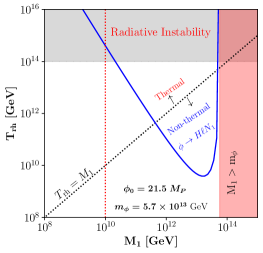
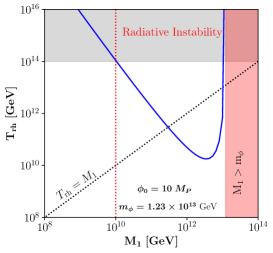
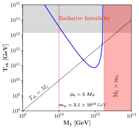
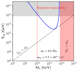
Figure 1: $T_{\text{rh}}$ as function of $M_{1}$ that yields the observed Baryon asymmetry via inflaton three body decays (blue line) from eq.(6.1.2) with ${\rm Im}\left(\sin^{2}z\right)=1$, for four different values of $\phi_{0}$. In the gray shaded region at the top loop corrections dominate the slope of the potential at $\phi_{0}$, invalidating our analysis of inflation. In the pink shaded region at the right $\phi\rightarrow H\ell N_{1}$ decays are kinematically forbidden. The dotted vertical red line indicates the minimal value of $M_{1}$ allowing thermal leptogenesis; the latter is only possible above the dotted black lines.

We saw in eq.(47) that $Y_{B-L}\gtrsim 10^{-10}$ is required in order to reproduce the observed BAU. The blue curves in Figs. 1 show the minimal value of $T_{\text{rh}}$ that allows to satisfy this condition, using eq.(6.1.2); for definiteness we have taken ${\rm Im}\left(\sin^{2}z\right)=1$. The upper left panel is for $\phi_{0}=21.5\ M_{P}$, leading to $m_{\phi}\simeq 5.7\times 10^{13}$ GeV; this large value of $\phi_{0}$, and correspondingly heavy inflaton, saturates the current upper bound on $r$. We exclude the gray shaded region, where $T_{\text{rh}}\gtrsim 2\times 10^{14}$ GeV, since here the Higgs loop will spoil the flatness of inflaton potential so that the inflationary predictions, which are based on the tree–level potential, cannot be trusted. The black dotted line corresponds to $T_{\text{rh}}=M_{1}$, above which $N_{1}$ particles thermalize, leading to thermal leptogenesis as investigated above. Note that when $T_{\text{rh}}>M_{1}$ the inflaton three-body decay could still generate $N_{1}$ particles, which however would not change their number density if they thermalize. The red dotted line corresponds to $M_{1}\simeq 10^{10}~{}\text{GeV}$, denoting the lower bound on $M_{1}$ for thermal leptogenesis.

Below the black dotted line, where $M_{1}>T_{\text{rh}}$, thermal leptogenesis is suppressed. In such case we find that the non–thermal channel via inflaton three–body decays might still be able to source the required BAU, as depicted by the blue line. When $M_{1}\to m_{\phi}$, the three-body decay is phase space closed, explaining why the blue curves suddenly go up.

We also show examples with smaller $\phi_{0}$ in Fig. 1: upper right panel $\phi_{0}=10\,M_{P}$, lower left panel $\phi_{0}=5\,M_{P}$ and lower right panel $\phi_{0}=2.5\,M_{P}$. For $\phi_{0}\lesssim 2.5\,M_{P}$, ${\rm Im}(\sin^{2}z)>1$ would be required, which would require some cancellation to occur in eq.(23).

Several comments are in order before we close this section. First, non–thermal leptogenesis via inflaton three–body decay investigated in this section is also viable for other inflation models (e.g. the Starobinsky Starobinsky:1980te and $\alpha$-attractor models Kallosh:2013hoa ) as long as the inflaton mass satisfies $m_{\phi}\gtrsim 10^{12}~{}\text{GeV}$ and $T_{\text{rh}}\gtrsim 10^{10}$ GeV. Second, it might also work in scenarios with a later epoch of matter domination by some very massive particle, e.g. a modulus field Drees:2017iod which predominantly decays into a pair of SM Higgs bosons. The above bound on $m_{\phi}$ should then be satisfied by this modulus field, and $T_{\text{rh}}$ refers to the temperature at the end of the modulus matter dominated epoch. Finally, for $m_{\phi}>2M_{1}$ the inflaton can also decay into pairs of RHNs, either via four–body decays, or via loop-induced two-body decays as commented in the end of Sec. 2. However, these processes have (even) smaller branching ratios than the three–body final state, which will therefore dominate non–thermal $N_{1}$ production in our bosonic reheating scenario.

6.2 Non–thermal Leptogenesis with Fermionic Reheating

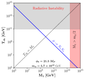
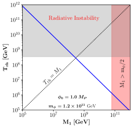
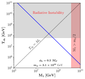
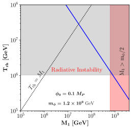
Figure 2: Parameter space for non–thermal leptogenesis if the inflaton predominantly decays into two $N_{1}$, for four different values of $\phi_{0}$ and hence of $m_{\phi}$. Above the blue lines the correct BAU can be generated non–thermally, see eq.(53). In the gray shaded regions our tree–level analysis of inflation is not reliable, while in the pink shaded regions $\phi\rightarrow N_{1}N_{1}$ decays are kinematically forbidden. Finally, below the dotted black lines $N_{1}$ does not attain thermal equilibrium.

In this section we assume that RHNs are produced via inflaton two body decays, $\phi\to N_{1}N_{1}$ Lazarides:1990huy ; Giudice:1999fb ; Asaka:1999jb ; Senoguz:2003hc ; Hahn-Woernle:2008tsk ; Antusch:2010mv ; these decays also reheat the universe. We saw above that in our inflationary scenario $T_{\text{rh}}$ is too low for thermal leptogenesis if the inflaton decays fermionically, except for a very limited region of parameter space at large $\phi_{0}$. Here we show that, even in our very simple type I see–saw model, the parameter space for leptogenesis is greatly expanded by this non–thermal $N_{1}$ production channel.

We will again assume that washout effects can be neglected if $T_{\text{rh}}<M_{1}$. The $B-L$ number yield after reheating can then simply be estimated as Kolb:1990vq ; Asaka:1999jb :

$$Y_{B-L}=\frac{n_{B-L}}{s}=\left[\frac{3}{2}\frac{T_{\text{rh}}}{m_{\phi}}\,\text{BR}(\phi\to N_{1}N_{1})\right]\,\epsilon_{1}\,.$$ (53)

The expression between the square parentheses denotes the yield of $N_{1}$ from inflaton decay, allowing for a general branching ratio BR for $\phi\rightarrow N_{1}N_{1}$; in our scenario of fermionic reheating with a hierarchical RHN spectrum, this branching ratio is unity, $\text{BR}=1$.

The allowed parameter space $(T_{\text{rh}},M_{1})$ is shown in Fig. 2. Here we consider $\phi_{0}=21.5\,M_{P}$ (upper left), corresponding to the largest allowed value compatible with the latest CMB experiments; $\phi_{0}=1.0\,M_{P}$ (upper right), $\phi_{0}=0.5\,M_{P}$ (lower left), and $\phi_{0}=0.1\,M_{P}$ (lower right). The gray regions are again excluded since radiative corrections from the $N_{1}$ loop would spoil the flatness of the inflaton potential near $\phi_{0}$. In the pink regions, $M_{1}>m_{\phi}/2$ hence $\phi\rightarrow N_{1}N_{1}$ is kinematically impossible. The blue line gives $Y_{B-L}=10^{-10}$ if the upper bound (6) on $\epsilon_{1}$ is used in eq.(53), i.e. below these lines the generated net lepton number is always too small. Finally, the black dotted lines again show $T_{\text{rh}}=M_{1}$, i.e. below these lines wash–out effects are small but above these lines $N_{1}$ thermalizes.

As remarked earlier, in a small region of parameter space with large $\phi_{0}$ and $T_{\text{rh}}>M_{1}$ (above the dotted black lines) thermal leptogenesis can occur. We note that the blue solid and black dotted lines intersect at

$$M_{1}^{\prime}=10^{3}\ {\text{GeV}}\;\cdot\sqrt{\frac{2}{3}\frac{m_{\phi}}{\text{GeV}}}\,.$$ (54)

Non–thermal leptogenesis can only occur for $M_{1}>M_{1}^{\prime}$. We see that for $\phi_{0}<M_{P}$ this is automatically satisfied by all points on the blue line where radiative corrections to the inflaton potential are under control. In this “small field” inflationary scenario, the maximal reheating temperature $T_{\rm rh}^{\rm max}\propto\phi_{0}^{5/2}$ for fermionic reheating Drees:2021wgd . Moreover, eqs. (53) and (6) show that $Y_{B-L}$ is maximal for maximal $M_{1}\simeq m_{\phi}/2$, hence the maximal $Y_{B-L}\propto T_{\rm rh}^{\rm max}\propto\phi_{0}^{5/2}$. In particular, for $\phi_{0}\leq 0.1M_{P}$, even non–thermal leptogenesis becomes impossible in our simple neutrino mass model.

Altogether the allowed range of $\phi_{0}$ leading to successful leptogenesis via $\phi\rightarrow N_{1}N_{1}$ decays, compatible with both CMB observations and neutrino oscillation data, is

$$0.1\,M_{P}\lesssim\phi_{0}\lesssim 21.5\,M_{P}\,.$$ (55)

In addition, the reheating temperature has to lie in the range

$$10^{6}~{}\text{GeV}\lesssim T_{\text{rh}}\lesssim 10^{10}~{}\text{GeV}\,,$$ (56)

while the mass of the lightest RHN should satisfy

$$10^{8}~{}\text{GeV}<M_{1}\lesssim 3\cdot 10^{13}~{}\text{GeV}\,.$$ (57)

7 Summary and Conclusions

Polynomial inflation is a very simple and predictive model. It fits current cosmic microwave background (CMB) data well, and makes testable predictions for the running of the spectral index and the tensor to scalar ratio.

A further necessary condition for a successful cosmological model is that it offers an explanation for the observed baryon asymmetry of the Universe (BAU). In this work we therefore revisit leptogenesis in the framework of polynomial inflation. We assume a type–I see–saw model with massless lightest neutrino, and therefore only two very heavy right–handed neutrinos. We show that even in this simple ansatz, in some part of the parameter space both the observed BAU and the neutrino oscillation data can be explained.

To that end we consider two different perturbative reheating scenarios. If the inflaton decays bosonically, the reheating temperature in our model can be as high as $T_{\text{rh}}\sim 10^{14}~{}\text{GeV}$, compatible with “plain vanilla” $N_{1}$ thermal leptogenesis. We also point out, for the first time, that even for $T_{\text{rh}}<M_{1}$, where thermal leptogenesis does not work, inflaton three–body decays of the inflaton into an SM Higgs boson, a RHN $N_{1}$ and an SM doublet lepton can lead to successful leptogenesis. As long as it is kinematically allowed, this decay will always occur if the primary inflaton decay mode is into two SM Higgs bosons; the required couplings are automatically present in the see–saw neutrino mass model, and can be expressed in terms of neutrino masses and a single complex mixing angle. We find that this three–body decay scenario is viable for inflaton mass $m_{\phi}\gtrsim 10^{12}~{}\text{GeV}$. In the polynomial inflation scenario this corresponds to $\phi_{0}\gtrsim 2.5~{}M_{P}$, but this novel mechanism should also be applicable to other models of large–scale inflation.

We also investigate the case where the inflaton primarily decays into two $N_{1}$. This fermionic decay mode leads to somewhat lower maximal reheating temperature. Thermal leptogenesis therefore works only in a rather small region of parameter space, but this inflaton decay mode allows non–thermal leptogenesis, if $\phi_{0}\gtrsim 0.1~{}M_{P}$, $M_{1}\gtrsim 3\cdot 10^{8}$ GeV and reheating temperature $T_{\text{rh}}\gtrsim 10^{6}~{}\text{GeV}$.

In conclusion, we have shown that a model with a renormalizable inflaton potential, in combination with a simple see–saw model with hierarchical masses of the right–handed neutrinos, allows successful thermal or non–thermal leptogenesis if inflation occurred at a field value $\phi\simeq\phi_{0}\gtrsim 0.1M_{P}$, corresponding to an Hubble parameter during inflation $H_{I}\gtrsim 2\cdot 10^{7}$ GeV. Deviating from our assumption of a very hierarchical spectrum of right–handed neutrinos should allow to construct viable models operating at much smaller energy scales. For example, it is known that thermal “resonant” leptogenesis, where two RHNs are nearly degenerate, can work at the TeV scale Pilaftsis:2003gt . It would be interesting to investigate this quantitatively.

Appendix A Inflaton Three–Body Decay into Right Handed Neutrino

In this appendix, we first calculate the branching ratio for inflaton three–body decays $\phi\to H\,\ell\,N_{1}$. Then we estimate the $B-L$ yield generated from the subsequent decay of $N_{1}$.

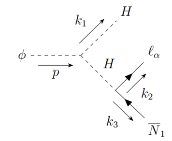
Figure 3: $N_{1}$ production via inflaton three–body decay.

Our basic assumption is that the main inflaton decay mode is into a pair of SM Higgs bosons via the coupling $\lambda_{12}$. The three–body decay shown in fig. 3 is then automatically allowed, as long as $M_{1}<m_{\phi}$. The RHN $N_{1}$ couples to the SM Higgs and lepton doublet through the Yukawa coupling $Y_{\alpha 1}\,\bar{\ell}_{\alpha}\tilde{H}N_{1}$, which is required for the explanation of the light neutrino masses.

We label the momenta for particles involved as follows:

$$\phi(p)\to H(k_{1})\,H(q)\to H(k_{1})\,\ell(k_{2})N_{1}(k_{3})\,,$$

The matrix element for a fixed lepton flavor $\alpha$ is given by

$$i\mathcal{M}_{\alpha}=2i\,\lambda_{12}\,\frac{i}{q^{2}-m_{H}^{2}}\,Y_{\alpha\,1}\bar{u}(k_{2})\text{v}(k_{3})\,.$$ (58)

After squaring and summing over lepton flavor and the $SU(2)$ index, this yields:

$$|\mathcal{M}|^{2} =\sum_{\alpha}4\,\lambda^{2}_{12}\left(Y^{\star}_{\alpha\,1}Y_{\alpha\,1}\right)\left(4k_{2}\cdot k_{3}-4M_{1}m_{\ell_{\alpha}}\right)\frac{1}{q^{4}}$$

$$\simeq 16\,\lambda^{2}_{12}k_{2}\cdot k_{3}\frac{1}{q^{4}}\sum_{\alpha}\left(Y^{\star}_{\alpha\,1}Y_{\alpha\,1}\right)\,.$$ (59)

In the second step we have neglected the small lepton mass. Note also that we assume unbroken $SU(2)$, hence all four (real) components of the Higgs doublet, and both charged and (light) neutral leptons, contribute.

The three–body phase space integral can be written as (see e.g. Appendix B of Barger:1987nn ):

$$\int d\Pi_{3}=\frac{m_{\phi}^{2}}{128\pi^{3}}\int^{1-\gamma}_{0}dx_{1}\int^{1-\frac{\gamma}{1-x_{1}}}_{1-x_{1}-\gamma}dx_{2}\,,$$ (60)

where $x_{i}=2E_{i}/m_{\phi}\,,\ i=1,2$, $E_{1}$ being the energy of the Higgs boson and $E_{2}$ that of the charged lepton in the inflaton rest frame, and $\gamma=M_{1}^{2}/m_{\phi}^{2}$. We have again neglected all masses in the final state except for that of the heavy RHN $N_{1}$. The product of $4-$vectors appearing in the squared matrix element (A) is related to $x_{1}$ via $2k_{2}\cdot k_{3}=m_{\phi}^{2}(1-x_{1})-M_{1}^{2}$.

Inserting eq. (A) into eq.(60) allows to compute the three–body decay rate:

$$\Gamma_{\text{3-body}}\equiv\Gamma_{\phi\to\ell HN_{1}} =\frac{1}{2m_{\phi}}\int d\Pi_{3}|\mathcal{M}|^{2}$$

$$=\frac{\lambda^{2}_{12}}{32\pi^{3}\,m_{\phi}}\int^{1-\gamma}_{0}dx_{1}\int^{1-\frac{\gamma}{1-x_{1}}}_{1-x_{1}-\gamma}dx_{2}\frac{\,(1-x_{1})-\gamma}{(1-x_{1})^{2}}\,\sum_{\alpha}\left(Y^{\star}_{\alpha\,1}Y_{\alpha\,1}\right)$$

$$=\frac{\lambda^{2}_{12}}{32\pi^{3}\,m_{\phi}}\sum_{\alpha}\left(Y^{\star}_{\alpha\,1}Y_{\alpha\,1}\right)\frac{1}{2}\left[\gamma^{2}+4\gamma-5-2(1+2\gamma)\ln\gamma\right]\,.$$ (61)

The branching ratio for the channel $\phi\to\ell N_{1}H$ is therefore

$$\text{BR}(\phi\to\ell N_{1}H) =\frac{\Gamma_{\text{3-body}}}{\Gamma_{\text{3-body}}+\Gamma_{\phi\to H^{\dagger}H}}\simeq\frac{\Gamma_{\text{3-body}}}{\Gamma_{\phi\to H^{\dagger}H}}$$

$$=\frac{m_{\phi}}{8\pi^{2}v^{2}}\left(m_{2}|\cos z|^{2}+m_{3}|\sin z|^{2}\right)\cdot f(\gamma)\,,$$ (62)

where we have used $\Gamma_{\phi\to H^{\dagger}H}=\lambda_{12}^{2}/(8\pi\,m_{\phi})$, and eq. (39) for $\sum_{\alpha}\left(Y^{\dagger}_{\alpha\,1}Y_{\alpha\,1}\right)$. The function $f(\gamma)$ is defined as:

$$f(\gamma)=\sqrt{\gamma}\left[\gamma^{2}+4\gamma-5-2(1+2\gamma)\ln\gamma\right]\,.$$ (63)

It peaks at $\gamma\simeq 0.0177$ with $f(\gamma)^{\text{max}}\simeq 0.456$.

If washout effects can be neglected, i.e. for $M_{1}>T_{\text{rh}}$, the generated $B-L$ yield is given by:

$$Y_{B-L} =\left[\frac{3}{4}\frac{T_{\text{rh}}}{m_{\phi}}\,\text{BR}(\phi\to\ell N_{1}H)\right]\,\epsilon_{1}$$

$$=\frac{3}{4}\frac{T_{\text{rh}}}{m_{\phi}}\left[\frac{m_{\phi}}{8\pi^{2}v^{2}}\left(m_{2}|\cos z|^{2}+m_{3}|\sin z|^{2}\right)\cdot f(\gamma)\right]$$

$$\hskip 14.22636pt\cdot\left[-\frac{3}{16\pi}\frac{M_{1}}{v^{2}}(m_{3}^{2}-m_{2}^{2})\frac{\text{Im}\left(\sin^{2}z\right)}{\left(m_{2}|\cos z|^{2}+m_{3}|\sin z|^{2}\right)}\right]$$

$$=-\frac{9}{512\pi^{2}}\frac{M_{1}\,T_{\text{rh}}}{v^{4}}(m_{3}^{2}-m_{2}^{2})\text{Im}\left(\sin^{2}z\right)\cdot f(\gamma)$$

$$\simeq-4.8\times 10^{-11}\left(\frac{m_{\phi}}{10^{11}\ \text{GeV}}\right)\left(\frac{T_{\text{rh}}}{10^{11}\ \text{GeV}}\right)\text{Im}\left(\sin^{2}z\right)\cdot\sqrt{\gamma}f(\gamma)\,.$$ (64)

In the third line we have utilized eq. (6).

Before closing this section, we note that RHNs could also be produced in the scattering of an inflaton and a daughter particle, $\phi H\to\ell N_{1}$ and $\phi\,\ell\to HN_{1}$. For $m_{\phi}>M_{1}$ this is possible even if the daughter particle in the initial state is soft, e.g. after thermalization with low reheating temperature. The rate for these scattering reactions involves the same product of couplings that appears in the three–body decay width. However the rate for inflaton scattering on a thermalized daughter particle is suppressed by a factor $T/m_{\phi}$ compared to the three–body decay rate; the rate for inflaton scattering on daughter particles before they thermalize is even smaller. We have therefore neglected these $2\to 2$ scattering reactions.

References

- (1) Planck collaboration, Planck 2018 results. X. Constraints on inflation, Astron. Astrophys. 641 (2020) A10 [1807.06211].
- (2) BICEP, Keck collaboration, Improved Constraints on Primordial Gravitational Waves using Planck, WMAP, and BICEP/Keck Observations through the 2018 Observing Season, Phys. Rev. Lett. 127 (2021) 151301 [2110.00483].
- (3) M. Drees and Y. Xu, Small field polynomial inflation: reheating, radiative stability and lower bound, JCAP 09 (2021) 012 [2104.03977].
- (4) M. Drees and Y. Xu, Large field polynomial inflation: parameter space, predictions and (double) eternal nature, JCAP 12 (2022) 005 [2209.07545].
- (5) J.B. Muñoz, E.D. Kovetz, A. Raccanelli, M. Kamionkowski and J. Silk, Towards a measurement of the spectral runnings, JCAP 05 (2017) 032 [1611.05883].
- (6) N. Bernal and Y. Xu, Polynomial inflation and dark matter, Eur. Phys. J. C 81 (2021) 877 [2106.03950].
- (7) M. Fukugita and T. Yanagida, Baryogenesis Without Grand Unification, Phys. Lett. B 174 (1986) 45.
- (8) W. Buchmuller, P. Di Bari and M. Plumacher, Leptogenesis for pedestrians, Annals Phys. 315 (2005) 305 [hep-ph/0401240].
- (9) L. Covi, E. Roulet and F. Vissani, CP violating decays in leptogenesis scenarios, Phys. Lett. B 384 (1996) 169 [hep-ph/9605319].
- (10) C.S. Fong, E. Nardi and A. Riotto, Leptogenesis in the Universe, Adv. High Energy Phys. 2012 (2012) 158303 [1301.3062].
- (11) G. Lazarides and Q. Shafi, Origin of matter in the inflationary cosmology, Phys. Lett. B 258 (1991) 305.
- (12) G.F. Giudice, M. Peloso, A. Riotto and I. Tkachev, Production of massive fermions at preheating and leptogenesis, JHEP 08 (1999) 014 [hep-ph/9905242].
- (13) T. Asaka, K. Hamaguchi, M. Kawasaki and T. Yanagida, Leptogenesis in inflaton decay, Phys. Lett. B 464 (1999) 12 [hep-ph/9906366].
- (14) T. Asaka, K. Hamaguchi, M. Kawasaki and T. Yanagida, Leptogenesis in inflationary universe, Phys. Rev. D 61 (2000) 083512 [hep-ph/9907559].
- (15) V.N. Senoguz and Q. Shafi, GUT scale inflation, nonthermal leptogenesis, and atmospheric neutrino oscillations, Phys. Lett. B 582 (2004) 6 [hep-ph/0309134].
- (16) F. Hahn-Woernle and M. Plumacher, Effects of reheating on leptogenesis, Nucl. Phys. B 806 (2009) 68 [0801.3972].
- (17) S. Antusch, J.P. Baumann, V.F. Domcke and P.M. Kostka, Sneutrino Hybrid Inflation and Nonthermal Leptogenesis, JCAP 10 (2010) 006 [1007.0708].
- (18) D. Croon, N. Fernandez, D. McKeen and G. White, Stability, reheating and leptogenesis, JHEP 06 (2019) 098 [1903.08658].
- (19) W. Occam, Quaestiones et decisiones in quattuor libros Sententiarum Petri Lombardi (1495).
- (20) Planck collaboration, Planck 2018 results. VI. Cosmological parameters, Astron. Astrophys. 641 (2020) A6 [1807.06209].
- (21) D.H. Lyth and A.R. Liddle, The primordial density perturbation: Cosmology, inflation and the origin of structure (2009).
- (22) M. Kawasaki, K. Kohri and N. Sugiyama, MeV scale reheating temperature and thermalization of neutrino background, Phys. Rev. D 62 (2000) 023506 [astro-ph/0002127].
- (23) S. Hannestad, What is the lowest possible reheating temperature?, Phys. Rev. D 70 (2004) 043506 [astro-ph/0403291].
- (24) I. Esteban, M.C. Gonzalez-Garcia, A. Hernandez-Cabezudo, M. Maltoni and T. Schwetz, Global analysis of three-flavour neutrino oscillations: synergies and tensions in the determination of , , and the mass ordering, JHEP 01 (2019) 106 [1811.05487].
- (25) J.A. Casas and A. Ibarra, Oscillating neutrinos and , Nucl. Phys. B 618 (2001) 171 [hep-ph/0103065].
- (26) A. Ibarra and G.G. Ross, Neutrino phenomenology: The Case of two right-handed neutrinos, Phys. Lett. B 591 (2004) 285 [hep-ph/0312138].
- (27) E.W. Kolb and M.S. Turner, The Early Universe, vol. 69 (1990), 10.1201/9780429492860.
- (28) S. Davidson and A. Ibarra, A Lower bound on the right-handed neutrino mass from leptogenesis, Phys. Lett. B 535 (2002) 25 [hep-ph/0202239].
- (29) A.A. Starobinsky, A New Type of Isotropic Cosmological Models Without Singularity, Phys. Lett. B 91 (1980) 99.
- (30) R. Kallosh and A. Linde, Universality Class in Conformal Inflation, JCAP 07 (2013) 002 [1306.5220].
- (31) M. Drees and F. Hajkarim, Dark Matter Production in an Early Matter Dominated Era, JCAP 02 (2018) 057 [1711.05007].
- (32) A. Pilaftsis and T.E.J. Underwood, Resonant leptogenesis, Nucl. Phys. B 692 (2004) 303 [hep-ph/0309342].
- (33) V.D. Barger and R.J.N. Phillips, Collider Physics (1987).