Not all Minorities are Equal: Empty-Class-Aware Distillation for
Heterogeneous Federated Learning

Abstract

Data heterogeneity, characterized by disparities in local data distribution across clients, poses a significant challenge in federated learning. Substantial efforts have been devoted to addressing the heterogeneity in local label distribution. As minority classes suffer from worse accuracy due to overfitting on local imbalanced data, prior methods often incorporate class-balanced learning techniques during local training. Despite the improved mean accuracy across all classes, we observe that empty classes-referring to categories absent from a client’s data distribution—are still not well recognized. This paper introduces FedED, a novel approach in heterogeneous federated learning that integrates both empty-class distillation and logit suppression simultaneously. Specifically, empty-class distillation leverages knowledge distillation during local training on each client to retain essential information related to empty classes from the global model. Moreover, logit suppression directly penalizes network logits for non-label classes, effectively addressing misclassifications in minority classes that may be biased toward majority classes. Extensive experiments validate the efficacy of FedED, surpassing previous state-of-the-art methods across diverse datasets with varying degrees of label distribution shift.

1 Introduction

Federated learning has emerged as a prominent distributed learning paradigm, lauded for its capability to train a global model without direct access to raw data (Konečnỳ et al., 2016; Li et al., 2020a; Kairouz et al., 2021). The traditional federated learning (FL) algorithm, such as FedAvg (McMahan et al., 2017), follows an iterative process of refining the global model. It achieves this by aggregating parameters from local models, which are initialized with the latest global model parameters and trained across diverse client devices. (Sheller et al., 2020; Li et al., 2020b; Chai et al., 2023).

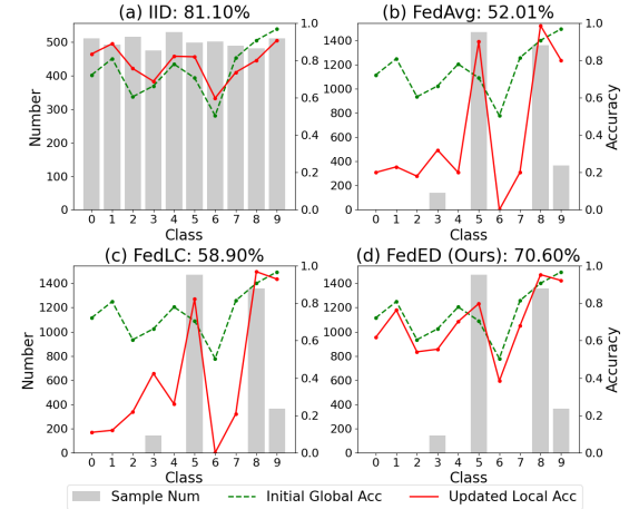
Figure 1: Class-wise accuracy of the initial global model and updated local model on heterogeneous CIFAR10 data distribution. (a) represents the result updating on IID local data with FedAvg (McMahan et al., 2017). (b-d) showcase the results updating on heterogeneous local data distribution with FedAvg (McMahan et al., 2017), FedLC (Zhang et al., 2022), and our FedED, respectively. The value (%) in each caption corresponds to the accuracy of the global model aggregated from updated local models.

In real-world scenarios, local client data always originate from diverse populations or organizations, displaying significant characteristics of data heterogeneity (Hsu et al., 2019; Yang et al., 2021; Reguieg et al., 2023). We particularly concentrate on the label distribution shift problem, a prevalent scenario in data heterogeneity that severely undermines the performance of federated learning (Zhang et al., 2023; Ye et al., 2023).

Typically, the local data consistently encompasses both majority and minority classes according to the number of samples in the class. As evidenced in prior studies (Zhang et al., 2022; Chen et al., 2022), the accuracy of minority classes notably decreases after the local update, signaling that the client model is entrenched in local overfitting. Consequently, this results in substantial performance degradation of the global model (Yeganeh et al., 2020; Li et al., 2020b; Liu et al., 2022). To address the problem of minority classes suffering from worse accuracy, previous methods often incorporate class-balanced learning techniques during local training (Zhang et al., 2022; Chen et al., 2022; Wang et al., 2023b; Shen et al., 2023). Some works (Zhang et al., 2022; Chen et al., 2022; Shen et al., 2023) advocate for calibrating logits according to the client data distribution to balance minority and majority classes. Moreover, FedBalance (Wang et al., 2023b) corrects the optimization bias among local models by calibrating their logits, with the help of an extra private weak learner on the client side. Nevertheless, these methods often focus on the imbalance among client-only observed classes, while neglecting the issue of empty classes. Empty classes, however, frequently occur in real-world clients’ data (Zhang et al., 2023).

For example, we compare the class-wise accuracy of the initial global model and updated local models using both the classic method FedAvg (McMahan et al., 2017) and one state-of-the-art method FedLC (Zhang et al., 2022). As depicted in Figure 1 (b) and (c), the updated local model exhibits a notable decline in accuracy for empty classes (e.g., categories 0, 1, 2, 4, 6, and 7) compared to the class-wise accuracy of the initial global model. In extreme cases, the accuracy even decreases close to zero (e.g., category 6). We posit this severe decline is attributed to the neglect of these empty classes. Although FedLC (Zhang et al., 2022) partially alleviates the performance decline for minority classes, particularly in classes 3 and 9, a significant gap persists compared to the IID (Independent and Identically Distributed) settings. This indicates that previous methods still often misclassify minority classes as majority classes.

Based on these findings, we present FedED, a novel approach comprising two pivotal components: empty-class distillation and logit suppression. The empty-class distillation aims to address the performance decline attributed to the disregard of empty classes. It distills vital information related to these classes from the global model for each client during local training. In addition, FedED incorporates logit suppression, which regulates the output logit for non-label classes. This process emphasizes minimizing the predicted logit values linked to the majority class when handling minority samples, which amplifies the penalty for the misclassification of minority classes. As shown in Figure 1 (d), FedED demonstrates significant effectiveness in mitigating the decline in accuracy in both empty and minority classes of the updated local model. As a result, FedED effectively mitigates overfitting within client models, leading to a significant performance of the global model. We experimentally demonstrate that FedED consistently outperforms the current state-of-the-art federated learning methods across various settings. We summarize our contributions as follows:

• We find that prior methods suffer from the empty classes and propose a new heterogeneous federated learning method, FedED, to distill empty-class-aware knowledge from the global model.

• FedED further presents logit suppression to address the misclassification of the minority classes, thereby enhancing the generalization of local models.

• Extensive results validate the effectiveness of both components in FedED, outperforming previous state-of-the-art methods across diverse datasets and different degrees of label heterogeneity.

2 Related Works

2.1 Heterogeneous Federated Learning

Federated Learning faces a major challenge known as data heterogeneity, also named Non-Identical and Independently Distribution (Kairouz et al., 2021; Luo et al., 2021; Shi et al., 2023b) (NON-IID). The classic federated learning algorithm, FedAvg (McMahan et al., 2017), experiences a significant decline in performance when dealing with data heterogeneity (Li et al., 2019; Acar et al., 2021).

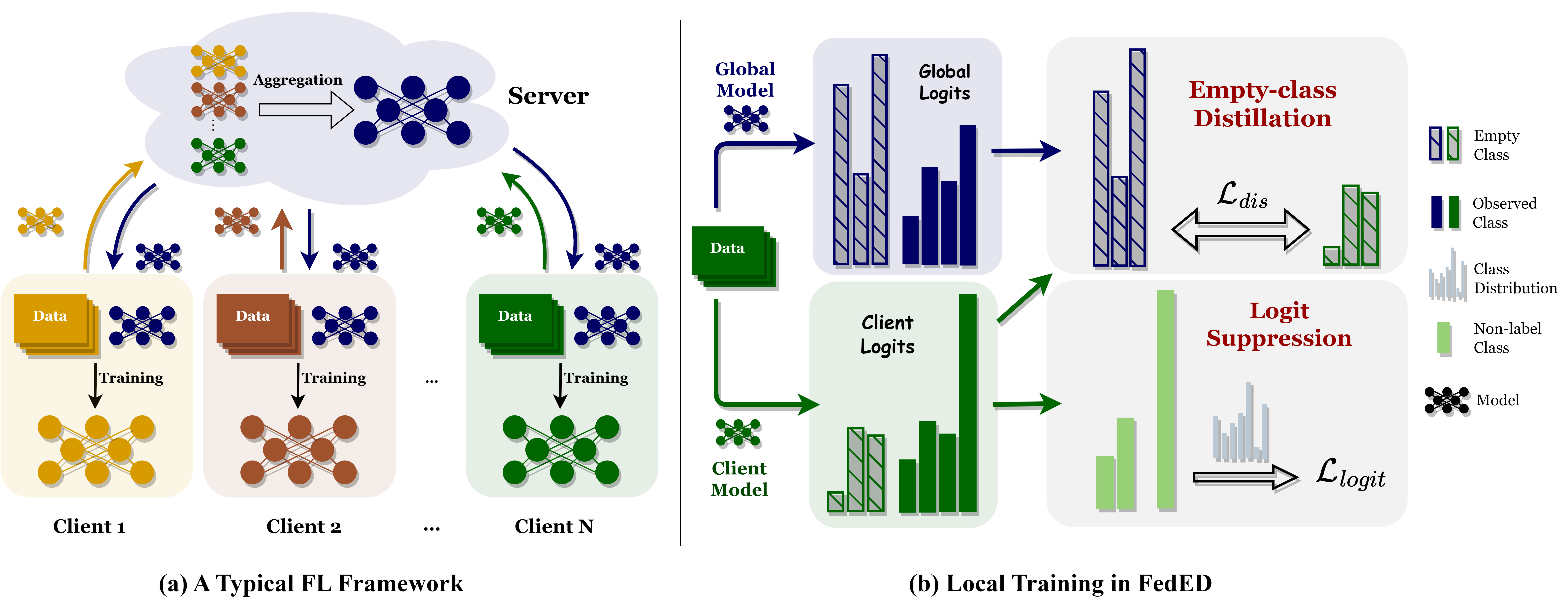
Figure 2: (a) represents the overall framework of typical federated learning. (b) showcases our method applied during local training. The empty-class distillation is employed to preserve the global knowledge of empty classes. The logit suppression is utilized to regularize the non-label class logit directly. The specific method details are presented in Section 3.3 and Section 3.4.

There are numerous studies dedicated to mitigating the adverse impacts of statistical heterogeneity. FedProx (Li et al., 2020b) utilizes a proximal term and SCAFFOLD (Karimireddy et al., 2020) employs a variance reduction approach to constrain the update direction of local models. On a different note, MOON (Li et al., 2021) and FedProc (Mu et al., 2023) utilize contrastive loss to enhance the agreement between local models and the global model. FedNTD (Lee et al., 2022) conducts local-side distillation only for the not-true classes to prevent overfitting while FedHKD (Chen et al., 2023) conducts local-side distillation on both logits and class prototypes to align the global and local optimization directions. Besides, FedLC (Zhang et al., 2022) and Calfat (Chen et al., 2022) introduce logit calibration based on the data distribution. However, they always focus on the client-only observed classes and neglect the consideration of empty classes. We find that empty classes cannot be merely treated as minority classes and propose FedED to effectively mitigate the decline in class-wise accuracy of empty classes.

2.2 Learning from Imbalanced Data

Imbalanced data distribution is pervasive in real-world scenarios, and a multitude of methods have been proposed to address the impact of data imbalance on model performance (Cui et al., 2019; Menon et al., 2021; Tan et al., 2020; Li et al., 2022; Ma et al., 2023). Existing approaches generally fall into two categories: re-weighting (Cui et al., 2019) and logit-adjustment (Menon et al., 2021; Tan et al., 2020). However, previous works primarily discuss scenarios with long-tailed distributions (Zeng et al., 2023; Xiao et al., 2023) These methods may not be directly applicable in federated learning due to the presence of empty classes in client data distribution. Our method, on the other hand, addresses both observed class imbalance and empty classes simultaneously, making them more practical in real-world scenarios.

2.3 Knowledge Distillation in Federated Learning

Knowledge Distillation (KD) is introduced to federated learning to aid with the issues that arise due to variations in resources and model constructions available to the clients (Jeong et al., 2018; Itahara et al., 2021; Wu et al., 2023). FedDF (Lin et al., 2020) and FedMD (Li & Wang, 2019) leverage the knowledge distillation to transfer the knowledge from multiple local models to the global model. However, these knowledge distillation methods always need a public dataset available to all clients on the server, presenting potential practical challenges. The latest methods, FEDGEN (Zhu et al., 2021b), DaFKD (Wang et al., 2023a), and DFRD (Luo et al., 2023), propose to train a generator on the server or client to enable data-free federated knowledge distillation. However, training the generator involves added computational complexity and can often be unstable in cases of extreme label distribution (Wu et al., 2023). In summary, most existing KD-based schemes either require a public dataset on the server or need costly computational efforts. However, our method employs knowledge distillation to protect the information of empty classes from the global model and does not introduce any additional requirements or a lot of computational overhead.

3 Method

3.1 Preliminaries

In federated learning, we consider a scenario with $N$ clients, where $\mathcal{D}_{i}$ represents the local training data of client $i$. The combined data $\mathcal{D}=\bigcup_{i=1}^{N}\mathcal{D}_{i}$ comprises all clients’ local data. These data distributions might differ across clients, encompassing situations where the local data of some clients only contain samples from a subset of all classes. The overarching goal is to address the optimization problem as follows:

$$\underset{\boldsymbol{\mathcal{\omega}}}{\lim}\left[{\mathcal{L}(\bf{\boldsymbol{\omega}})}\overset{def}{=}\sum_{i=1}^{N}{\frac{|\mathcal{D}_{i}|}{|\mathcal{D}|}{\mathcal{L}_{i}}(\bf{\boldsymbol{\omega}})}\right],$$ (1)

where $\mathcal{L}_{i}({\bf\boldsymbol{\omega}})=\mathbb{E}_{(x,y)\sim\mathcal{D}_{i}}[{\ell}_{i}(f({\bf\boldsymbol{\omega}};x),y)]$ is the empirical loss of the $i$-th client. $f({\bf\boldsymbol{\omega}};x)$ is the output of the model when the input $x$ and model parameter ${\bf\boldsymbol{\omega}}$ are given, and ${\ell}_{i}$ is the loss function of the $i$-th client. $|\mathcal{D}_{i}|$ is the number of samples on $\mathcal{D}_{i}$, $|\mathcal{D}|$ is the number of samples on $\mathcal{D}$. Here, FL expects to learn a global model that can perform well on the entire data $\mathcal{D}$.

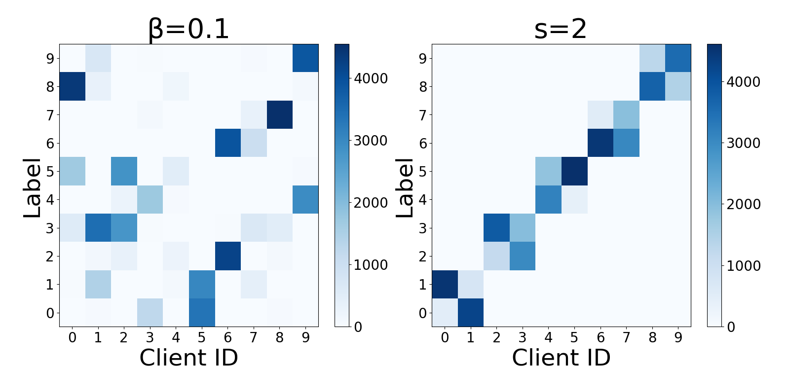
Figure 3: Visualization of the heterogeneous CIFAR10 data distribution among 10 clients. Left: the Dirichlet-based label distribution shift ($\beta$ = 0.05); Right: the quantity-based label distribution shift ($s$ = 2).

3.2 Motivation

When the local data $\{\mathcal{D}_{\textit{i}}\}^{N}_{i=1}$ show label distribution shifts, as illustrated in Figure 3, the data quantities of different categories are imbalanced on each client, leading the client models to excessively fit their respective local data distributions. This overfitting phenomenon causes divergence during model aggregation and subsequently results in inferior global performance (Yeganeh et al., 2020; Li et al., 2020b; Liu et al., 2022). To deal with the imbalance between minority and majority classes, previous methodologies (Zhang et al., 2022; Shen et al., 2023) suggest calibrating logits based on the local data distribution, outlined as follows:

$$\mathcal{L}_{\bf cal}=-\mathbb{E}_{(x,y)\sim\mathcal{D}_{i}}\log\left(\frac{p(y)\cdot e^{f({\bf\boldsymbol{\omega}};x)\left[\it{y}\right]}}{\sum_{c}{p(c)\cdot e^{f({\bf\boldsymbol{\omega}};x)[\it{c}]}}}\right),$$ (2)

where $p(y)$ signifies the probability of label class $y$ occurring within the client’s data distribution, while $f({\bf\boldsymbol{\omega}};x)[c]$ denotes the logit output for the c-th category. The calibration technique weights the outputs for all classes in the denominator by $p(c)$. However, the probability $p(m)$ for the empty class in the client data distribution equates to zero, which leads to the weighting term for the empty category, ${p(m)\cdot e^{f({\bf\boldsymbol{\omega}};x)[m]}}$, also becoming zero. As a result, local models prioritize learning the observed classes, gradually disregarding information associated with the empty categories during local training. This gradual shift causes the updated direction of local models to deviate from that of the global model over time. It’s crucial to acknowledge that treating the empty class merely as a unique minority class is insufficient, an oversight prevalent in prior methodologies. We assert that this drawback significantly contributes to severe instances of local overfitting.

Our empirical observations reveal a substantial decrease in class-wise accuracy for empty classes (such as categories 0, 1, 2, 4, 6, and 7) after the local update, as illustrated in Figure 1 (b) and (c). Notably, in specific cases (such as category 6), this accuracy even drops close to zero. Moreover, the updated class-wise accuracy for the minority classes (e.g., category 3) continues to display a notable decline, maintaining a significant gap compared to the IID scenario. Thus, we aim to develop different objectives to alleviate these two issues, respectively.

3.3 Empty-class Distillation

Motivated by the above observations and analyses of empty classes, we propose to prevent the disappearance of information related to empty classes during local training. The global model harbors valuable insights, particularly regarding the prediction of empty classes, making it an exceptional teacher for each client. Hence, we introduce empty-class distillation, aimed at preserving the global perspective of empty classes for clients through knowledge distillation. To achieve this, we utilize the Kullback-Leibler Divergence loss function, as outlined below:

$$\mathcal{L}_{\bf dis}=\mathbb{E}_{(x,y)\sim\mathcal{D}_{i}}\sum_{o\in\mathbb{O}}{q^{g}(o;x)\log\left[\frac{q(o;x)}{q^{g}(o;x)}\right]},$$ (3)

$$\text{where}\;q(o;x)=\frac{\exp(f({\bf\boldsymbol{\omega}};x)[o])}{\sum_{c\in\mathbb{O}}{\exp(f({\bf\boldsymbol{\omega}};x)[c])}}$$

denotes the output for the $o$-th class of the local model using softmax within the empty classes, and $q^{g}(o;x)=\frac{\exp(f({\bf\boldsymbol{\omega}^{g}};x)[o])}{\sum_{c\in\mathbb{O}}{\exp(f({\bf\boldsymbol{\omega}^{g}};\it{x})[c]}}$ denotes the same for the global model. $\mathbb{O}$ represents the set that contains all empty classes within the local client data and $\boldsymbol{\omega}^{g}$ denotes the parameters of the global model.

This loss function enforces the local model to replicate the global model’s outputs within empty classes, thus maintaining the predictive capability for empty categories. Furthermore, the computational load imposed by this loss function is minimal, enhancing its practicality in implementation.

3.4 Logit Suppression

The previous methods often misclassify minority classes as majority classes, a factor that needs alleviation to further improve the generalization of local models. It’s evident that in the model’s output for minority samples, the majority class tends to have a higher logit value, ultimately leading to the misclassification of minority classes. Hence, we implement regularization on non-label class logits to emphasize penalizing the majority class output of minority samples. To avoid non-trivial optimization over direct logits, we aim to minimize the following objective for each class,

$$\mathcal{L}^{c}_{\bf logit}=\log\left(\mathbb{E}_{(x,y)\sim\mathcal{D}_{i}}\mathbb{I}({y\neq c})\cdot e^{f(\boldsymbol{\omega};x)[c]}\right),$$ (4)

where $\mathbb{I}$ is an indicator function with value 1 when ${y\neq c}$. Since minority samples are prone to be more frequently misclassified into majority classes, the higher weight should be assigned to the logits of majority categories in non-labeled outputs. Therefore, we weight the loss function $\mathcal{L}^{c}_{\bf logit}$ using the probability of occurrence $p(c)$ for each class as follows:

$$\mathcal{L}_{\bf logit}=\sum_{c\not\in\mathbb{O}}p(c)\cdot\mathcal{L}^{c}_{\bf logit}.$$ (5)

This adaptation prompts the learning process to pay more attention to the penalty for incorrectly classifying minority class samples as majority classes. As a result, the model is encouraged to refine its prediction across diverse classes, thereby improving its overall generalization capability.

Table 1: Performance overview for different degrees of Dirichlet-based label distribution shift. All results are (re)produced by us and are averaged over 3 runs (mean ± std). Bold is the best result, underline is the second-best.

Method	MNIST			CIFAR10			CIFAR100			TinyImageNet
	$\beta=0.5$	$\beta=0.1$	$\beta=0.05$	$\beta=0.5$	$\beta=0.1$	$\beta=0.05$	$\beta=0.5$	$\beta=0.1$	$\beta=0.05$	$\beta=0.5$	$\beta=0.1$	$\beta=0.05$
FedAvg (McMahan et al., 2017)	98.96 $\pm 0.00$	96.69 $\pm 0.00$	94.77 $\pm 0.44$	91.46 $\pm 0.55$	82.00 $\pm 0.75$	62.90 $\pm 0.95$	72.22 $\pm 0.34$	66.18 $\pm 0.35$	62.13 $\pm 0.09$	47.02 $\pm 0.40$	39.90 $\pm 0.27$	35.21 $\pm 0.47$
FedProx (Li et al., 2020b)	98.93 $\pm 0.00$	96.42 $\pm 0.00$	94.95 $\pm 0.24$	92.24 $\pm 0.78$	82.65 $\pm 1.33$	63.14 $\pm 0.41$	72.65 $\pm 0.60$	66.61 $\pm 0.22$	62.23 $\pm 0.20$	45.76 $\pm 0.50$	40.26 $\pm 0.51$	35.22 $\pm 0.17$
MOON (Li et al., 2021)	99.18 $\pm 0.01$	96.94 $\pm 0.12$	93.39 $\pm 0.21$	92.13 $\pm 0.35$	83.38 $\pm 0.43$	61.34 $\pm 0.77$	72.87 $\pm 0.11$	66.12 $\pm 0.32$	60.45 $\pm 0.41$	42.26 $\pm 0.36$	36.88 $\pm 0.53$	33.61 $\pm 0.35$
FedEXP (Jhunjhunwala et al., 2023)	97.57 $\pm 0.49$	91.59 $\pm 0.48$	92.54 $\pm 1.08$	92.31 $\pm 0.52$	83.48 $\pm 1.15$	63.22 $\pm 0.51$	72.41 $\pm 0.39$	66.74 $\pm 0.19$	62.24 $\pm 0.18$	47.00 $\pm 0.23$	40.58 $\pm 0.15$	34.95 $\pm 0.18$
FedLC (Zhang et al., 2022)	98.97 $\pm 0.01$	95.59 $\pm 0.05$	85.56 $\pm 0.18$	91.98 $\pm 0.63$	82.24 $\pm 0.53$	57.31 $\pm 0.97$	72.69 $\pm 0.30$	66.20 $\pm 0.20$	59.18 $\pm 0.11$	48.01 $\pm 0.21$	41.46 $\pm 0.37$	35.56 $\pm 0.58$
FedRS (Li & Zhan, 2021)	99.03 $\pm 0.00$	96.67 $\pm 0.01$	94.60 $\pm 0.40$	92.55 $\pm 0.68$	83.95 $\pm 0.35$	63.17 $\pm 0.57$	72.99 $\pm 0.20$	66.84 $\pm 0.25$	62.19 $\pm 0.06$	47.95 $\pm 0.43$	41.77 $\pm 0.25$	35.82 $\pm 0.20$
FedSAM (Qu et al., 2022)	99.21 $\pm 0.00$	97.24 $\pm 0.00$	95.17 $\pm 0.42$	92.37 $\pm 1.33$	81.19 $\pm 0.32$	63.11 $\pm 1.05$	72.96 $\pm 0.25$	67.50 $\pm 0.19$	61.32 $\pm 0.14$	48.43 $\pm 1.42$	43.96 $\pm 1.02$	41.14 $\pm 0.23$
FedNTD (Lee et al., 2022)	99.15 $\pm 0.04$	96.67 $\pm 0.17$	94.30 $\pm 0.71$	92.46 $\pm 0.19$	83.23 $\pm 0.22$	68.71 $\pm 0.27$	73.43 $\pm 0.15$	68.00 $\pm 0.50$	63.71 $\pm 0.19$	48.02 $\pm 1.05$	45.11 $\pm 0.21$	40.65 $\pm 0.26$
FedED	99.23 $\pm 0.00$	97.24 $\pm 0.00$	95.56 $\pm 0.12$	92.66 $\pm 0.14$	84.35 $\pm 0.04$	75.71 $\pm 0.28$	73.49 $\pm 0.80$	69.02 $\pm 0.18$	65.71 $\pm 0.01$	48.54 $\pm 0.12$	47.73 $\pm 0.13$	45.23 $\pm 0.15$

3.5 Overall Objective

As of now, we have elaborated extensively on our strategy to tackle the problem of overlooking empty classes in previous methods through knowledge distillation. Moreover, we mitigate the decrease in minority class of the updated local model by regulating non-label logits directly, to further alleviate local overfitting issues. In summary, we propose the comprehensive method named FedED, whose objective is as follows:

$$\mathcal{L}({\bf\boldsymbol{\omega}})=\mathcal{L}_{\bf cal}+\lambda\cdot\mathcal{L}_{\bf dis}+\mathcal{L}_{\bf logit},$$ (6)

where $\lambda$ is a non-negative hyperparameter to control the contribution of empty-class distillation. In the loss function of our FedED, we attain new knowledge from the observed class in local data distribution using the $\mathcal{L}_{\bf cal}$ and $\mathcal{L}_{\bf logit}$. In the meanwhile, we preserve the previous knowledge on the empty classes by following the global model’s perspective using the $\mathcal{L}_{\bf dis}$. By combining empty-class distillation and logit suppression, FedED can effectively manipulate various levels of data heterogeneity. The complete flowchart of our method is illustrated in Figure 2 and the pseudo-code can be found in Appendix B.

4 Experiments

4.1 Setups

Datasets. We evaluate the effectiveness of our approach in image classification datasets including MNIST (Deng, 2012), CIFAR10 (Krizhevsky, 2009), CIFAR100 (Krizhevsky, 2009), and TinyImageNet (Le & Yang, 2015). To simulate label distribution shift, we follow the settings in (Li et al., 2022) and introduce two commonly used forms of label shift: Dirichlet-based and quantity-based. The diversity in label distribution is illustrated in Figure 3. In the quantity-based label shift, data is grouped by label and allocated into shards with imbalanced quantities. $s$ represents the number of shards per client, which is used to control the level of label distribution shift (Lee et al., 2022). This setting leads to each client’s training data exclusively encompassing a subset of all labels, resulting in the presence of empty classes. In the Dirichlet-based label shift, clients receive samples for each class based on the Dirichlet distribution (Zhu et al., 2021a), denoted as $D(\beta)$. Here, the parameter $\beta$ controls the degree of heterogeneity, with lower values indicating higher heterogeneity. Notably, under the Dirichlet-based label shift, each client’s training data may include majority classes, minority classes, and even empty classes, which is more practical.

Models and baselines. Following a prior study (Shi et al., 2023a), our primary network architecture for all experiments, except MNIST, predominantly relies on MobileNetV2 (Sandler et al., 2018). For the MNIST, we adopt a deep neural network (DNN) containing three fully connected layers as the backbone. Our baseline models encompass conventional approaches to tackle data heterogeneity issues, including FedProx (Li et al., 2020b), MOON (Li et al., 2021), FedSAM (Qu et al., 2022), and FedEXP (Jhunjhunwala et al., 2023). To ensure a fair comparison, we assess our method against FedRS (Li & Zhan, 2021), FedLC (Zhang et al., 2022), and FedNTD (Lee et al., 2022), which also focus on addressing label distribution shift in federated learning.

Table 2: Performance overview for quantity-based label distribution shift setting. $s$ presents the number of shards per client.

Method	CIFAR10	CIFAR100	TinyImageNet
	$s=2$	$s=20$	$s=40$
FedAvg (McMahan et al., 2017)	44.63$\pm 0.77$	63.14$\pm 0.03$	30.28$\pm 0.12$
FedProx (Li et al., 2020b)	48.65$\pm 0.59$	62.10$\pm 0.10$	28.14$\pm 0.93$
MOON (Li et al., 2021)	38.24$\pm 1.00$	57.33$\pm 0.06$	26.25$\pm 0.73$
FedEXP (Jhunjhunwala et al., 2023)	41.11$\pm 0.26$	62.61$\pm 0.06$	29.38$\pm 0.19$
FedLC (Zhang et al., 2022)	55.14$\pm 0.26$	61.56$\pm 0.03$	26.29$\pm 1.00$
FedRS (Li & Zhan, 2021)	42.20$\pm 1.49$	61.53$\pm 0.03$	28.31$\pm 0.06$
FedSAM (Qu et al., 2022)	36.97$\pm 1.18$	63.50$\pm 0.01$	37.55$\pm 0.10$
FedNTD (Lee et al., 2022)	67.35$\pm 0.19$	63.74$\pm 0.01$	37.19$\pm 0.07$
FedED	68.03$\pm 0.$18	64.95$\pm 0.01$	43.97$\pm 0.04$

Implementation Details. We set the number of clients N to 10 and implement full client participation. We run 100 communication rounds for all experiments on the CIFAR10/100 datasets and 50 communication rounds on the MNIST and TinyImageNet datasets. Within each communication round, local training spans 5 epochs for MINST and 10 epochs for the other datasets. We employ stochastic gradient descent (SGD) optimization with a learning rate of 0.01, a momentum of 0.9, and a batch size of 64. Weight decay is set to $10^{-5}$ for MNIST and CIFAR10 and $10^{-4}$ for CIFAR100 and TinyImageNet. The augmentation for all CIFAR and TinyImageNet experiments is the same as existing literature (Cubuk et al., 2019). The hyperparameter $\lambda$ of FedED in Equation 6 is set to 0.1 for MNIST and CIFAR10, while it is set to 0.5 for CIFAR100 and TinyImageNet. To ensure reliability, we conduct three trials for each experimental setting and report the mean accuracy and standard deviation in the tables.

4.2 Results

Results Under Various levels of Data Heterogeneity and Datasets. Table 1 presents the performance results of various methods with different levels of Dirichlet-based label distribution shift ($\beta\in\{0.5,0.1,0.05\}$). Our method consistently achieves notably higher accuracy compared to other state-of-the-art (SOTA) methods across all scenarios. As the degree of data heterogeneity increases, competing methods struggle to maintain their performance levels. Specifically, FedLC (Zhang et al., 2022) experiences a substantial decline, dropping even below the performance of the classic method FedAvg when $\beta=0.05$. This decline stems from each client having numerous empty classes in extreme cases, a factor overlooked by FedLC (Zhang et al., 2022). Conversely, our method consistently upholds excellent performance, especially in highly heterogeneous label distribution scenarios. For instance, in the case of the CIFAR10 dataset with $\beta=0.05$, our method achieves an impressive test accuracy of 75.71%, surpassing FedAvg by 12.81%. This outcome highlights the efficacy of our approach in remedying the accuracy decline observed in both empty and minority classes, effectively mitigating instances of local overfitting. Additionally, we present the performance of these methods for quantity-based label distribution shift in Table 2, further emphasizing the superiority of our method.

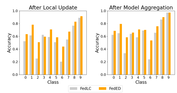
Figure 4: Comparison of class-wise accuracy after local update and after model aggregation with Dirichlet-based label shift ($\beta=0.05$) on CIFAR10 dataset.

Class-wise Accuracy. To evaluate the effectiveness of our approach, we conduct a comparative analysis of class-wise accuracy before and after local updates using our method, classic method FedAvg (McMahan et al., 2017), and one SOTA method FedLC (Zhang et al., 2022). To ensure a fair comparison, we employ the same well-trained federated model as the initial global model. Then the central server distributes the model parameter to all clients. Then, we train the local models using FedAvg (McMahan et al., 2017), FedLC (Zhang et al., 2022), and our method with the same local data distribution. As depicted in Figure 1, the results are consistent with the observations in Section 3.2. Furthermore, we compare the average class-wise accuracy for all clients after the local update and the class-wise accuracy for the aggregated global model of our approach with FedLC (Zhang et al., 2022), as demonstrated in Figure 4. Our method’s class-wise accuracy surpasses that of FedLC (Zhang et al., 2022) after both local update and model aggregation. These outcomes highlight how our method effectively enhances the performance of minority and empty classes, leading to an overall enhancement in the global model’s performance.

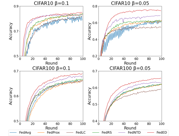
Figure 5: The test accuracy in each communication round during training for different levels of Dirichlet-based label shift ($\beta\in\{0.1,0.05\}$) on CIFAR10 and CIFAR100 datasets.

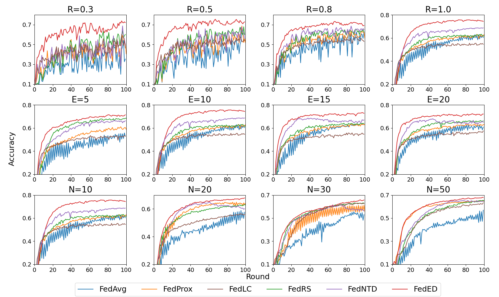
Figure 6: Sensitivity analysis on the client participating rate $\mathbf{R}$, local epochs $\mathbf{E}$, and client numbers $\mathbf{N}$. Each figure separately shows the convergence curve with Dirichlet-based label shift ($\beta=0.05$) on CIFAR10 dataset with $\mathbf{R}$ in $\{0.3,0.5,0.8,1.0\}$, $\mathbf{E}$ in $\{5,10,15,20\}$ and $\mathbf{N}$ in $\{10,20,30,50\}$.

Communication Efficiency. Figure 5 illustrates the accuracy in each communication round throughout the training process. Our method showcases quicker convergence and higher accuracy when compared to the other five methods. Unlike its counterparts, our approach displays a more consistent upward trend. Moreover, compared to other methods, our approach exhibits a larger improvement as the heterogeneity of the data increases. These outcomes underscore the substantial communication efficiency of our method in contrast to other approaches.

Table 3: Results of different methods under various backbones with Dirichlet-based label shift on CIFAR10 dataset.

Method	ResNet18		ResNet32		MobileNetV2
	$\beta$=0.1	$\beta$=0.05	$\beta$=0.1	$\beta$=0.05	$\beta$=0.1	$\beta$=0.05
FedAvg (McMahan et al., 2017)	73.84	58.54	79.38	55.41	82.00	62.90
FedProx (Li et al., 2020b)	74.68	58.14	80.60	62.51	82.65	63.14
MOON (Li et al., 2021)	74.04	55.41	76.91	51.85	83.38	61.34
FedEXP (Jhunjhunwala et al., 2023)	72.80	58.04	78.36	53.35	83.48	63.22
FedLC (Zhang et al., 2022)	73.15	48.94	77.71	55.41	82.24	57.31
FedRS (Li & Zhan, 2021)	76.38	57.47	82.03	66.87	83.95	63.17
FedSAM (Qu et al., 2022)	68.42	55.42	75.66	58.88	81.19	63.11
FedNTD (Lee et al., 2022)	76.76	60.01	79.75	65.96	83.23	68.71
FedED	78.00	68.33	82.44	68.84	84.35	75.71

4.3 Analysis

Impact of Participating Rates. To begin with, we analyze our model’s performance against state-of-the-art methods across varying client participation rates. Unless specified otherwise, our experiments focus on the CIFAR10 dataset with a Dirichlet-based heterogeneity parameter of $\beta=0.05$. Initially, we set the client participation rate $R$ within the range $\{0.3,0.5,0.8,1.0\}$ and assess the accuracy of our method alongside other state-of-the-art methods in each communication round. As illustrated in the top row of Figure 6, our method consistently outperforms other approaches across all participation rates, showcasing a faster convergence rate. Notably, as the participation rate decreases, particularly at $R=0.3$, several methods display highly unstable convergence. This instability is expected, as a lower client participation rate amplifies the divergence between randomly participating clients and the global model, resulting in erratic convergence. In contrast, our method exhibits a relatively stable convergence trend.

Table 4: Results under varying numbers of communication rounds with Dirichlet-based label shift on CIFAR10 dataset.

Method	40 comm		60 comm		80 comm
	$\beta$=0.1	$\beta$=0.05	$\beta$=0.1	$\beta$=0.05	$\beta$=0.1	$\beta$=0.05
FedAvg (McMahan et al., 2017)	74.62	53.44	78.59	56.71	80.72	59.10
FedProx (Li et al., 2020b)	78.59	57.67	81.63	61.84	82.88	61.96
MOON (Li et al., 2021)	78.23	52.84	81.73	57.11	82.91	61.35
FedEXP (Jhunjhunwala et al., 2023)	75.90	54.14	79.69	55.98	81.51	60.01
FedLC (Zhang et al., 2022)	75.74	53.06	77.22	53.77	80.22	55.75
FedRS (Li & Zhan, 2021)	79.10	60.99	81.13	63.16	82.94	64.28
FedSAM (Qu et al., 2022)	69.02	50.05	75.42	55.85	78.38	60.79
FedNTD (Lee et al., 2022)	81.26	65.75	82.23	66.48	82.95	67.91
FedED	82.54	72.90	83.82	74.34	84.30	75.25

Impact of Local Epochs. In this analysis, we investigate variations in the number of local epochs per communication round, represented as $E$, considering values from $\{5,10,15,20\}$. An intriguing observation emerges, particularly noticeable when $E$ equals 20: several methods, notably FedNTD (Lee et al., 2022), exhibit declining accuracy in the later stages of training, as depicted in the second row of Figure 6. This decline is attributed to larger $E$ values, making these models more susceptible to overfitting local data distribution as training progresses. In contrast, our method sustains a consistent and improving performance even with larger $E$ values and consistently outperforms all other methods.

Impact of Client Numbers. To underscore the resilience of our method in scenarios involving an increasing number of clients, we divided the CIFAR10 dataset into 10, 20, 30, and 50 clients, showcasing their convergence curves in the final row of Figure 6. Remarkably, our method consistently outperforms the baseline methods, regardless of the number of clients. An interesting trend emerges where, with the expanding number of clients, many methods exhibit slower and less stable convergence. In contrast, FedED maintains a consistent trend of rapid and stable convergence across these varied client counts.

Table 5: Effectiveness of each loss function in FedED with Dirichlet-based label shift ($\beta=0.05$) on various datasets. (The value) represents the improvement over the first row, FedLC (Zhang et al., 2022).

$\mathcal{L}_{\bf dis}$	$\mathcal{L}_{\bf logit}$	CIFAR10	CIFAR100	TinyImageNet
✗	✗	55.38	59.18	34.99
✗	✓	70.25(+14.87)	64.24(+5.06)	39.04(+4.05)
✓	✗	71.53(+16.15)	65.28(+6.10)	44.90(+9.91)
✓	✓	75.71(+20.33)	65.71(+6.53)	45.23(+10.24)

Impact of Different Backbones. Apart from MobileNetV2, we conducted experiments using ResNet18 and ResNet32. The heterogeneity parameter, denoted as $\beta$, is set to 0.1 and 0.05. The results are presented in Table 3, demonstrating that our method, FedED, consistently outperforms the baseline methods. These experiments demonstrate the potential of FedED in real-world federated learning scenarios employing various backbone architectures.

Impact of Different Numbers of Communication Round. In real-world scenarios, limitations frequently arise concerning the communication rounds. To address this, we conducted tests to evaluate performance across various communication round limits on the CIFAR10 dataset, considering $\beta=0.1$ and $\beta=0.05$. The results, outlined in Table 4, reveal a notable trend: as the communication rounds decrease, the accuracy of most methods experiences a significant decline. However, our method stands out by maintaining a high level of accuracy even with a reduced number of communication rounds. This highlights the robustness of FedED in scenarios with limited communication rounds.

Table 6: Results of the combination of FedED with other methods with Dirichlet-based label shift ($\beta=0.05$) on various datasets. (The value) represents the performance gains.

Method	CIFAR10	CIFAR100	TinyImageNet
FedAvg (McMahan et al., 2017)	62.90	62.13	36.15
FedED	75.71(+12.81)	65.71(+3.58)	45.23(+9.08)
FedEXP (Jhunjhunwala et al., 2023)	63.22	62.24	34.95
+ FedED	75.80(+12.58)	65.94(+3.70)	44.76(+9.81)
FedSAM (Qu et al., 2022)	63.11	61.32	41.14
+ FedED	75.92(+12.81)	65.46(+4.14)	48.12(+6.98)

Effectiveness of Different Objectives. Our approach comprises two key objectives: empty-classes distillation and logit suppression. To gauge the effectiveness of each objective, we conducted experiments on CIFAR10 with $\beta=0.05$, presenting the results in Table 5. In comparison to FedLC (Zhang et al., 2022), empty-classes distillation and logit suppression both showcase notable performance improvements, which demonstrates the effectiveness of our two key objectives. Additionally, when combined with the empty-classes distillation, the logit suppression further amplifies the overall model performance.

Combination with Other Techniques. In this section, we integrated our method with two SOTA methods, FedEXP (Jhunjhunwala et al., 2023) and FedSAM (Qu et al., 2022), detailed in Table 6. The combination of our method with FedEXP (Jhunjhunwala et al., 2023) and FedSAM (Qu et al., 2022) results in improved performance. This enhancement is reasonable because FedEXP focuses on optimizing the server update for an improved learning rate, and FedSAM emphasizes local gradient descent to achieve a smoother loss landscape. These elements complement well with our core idea, which finally results in enhanced performance when combined.

5 Conclusion

We identify that prior federated learning methods always perform poorly in minority classes, especially the empty ones, under heterogeneous label distribution across clients. To tackle these challenges, we present FedED—an innovative methodology integrating empty-class distillation and logit suppression. The empty-class distillation distills pertinent knowledge concerning empty classes from the global model to each client, while logit suppression is introduced to directly regularize non-label class logits, addressing the imbalance among majority and minority classes. Extensive results validate the effectiveness of both components, surpassing existing methods across diverse datasets and varying degrees of label distribution heterogeneity. In future work, we will analyze the convergence properties of FedED.

Appendix A Additional experimental results

Robustness to Hyperparameter $\lambda$. To showcase the robustness of our method concerning hyperparameter selection, we conducted experiments using different values of $\lambda$ on CIFAR10 and CIFAR100 datasets. The findings, presented in Table LABEL:fig:_diff_beta, illustrate that our method exhibits insensitivity to the parameter $\lambda$. Across $\lambda\in\{0.05,0.1,0.25,0.5,1\}$, our method consistently achieves approximately 75% accuracy on CIFAR10 and 65.5% on CIFAR100. This consistent performance highlights our method’s ability to deliver stable results regardless of variations in $\lambda$ values, underscoring its robustness to hyperparameter changes.

Table 7: Results under different values of hyperparameter $\lambda$ with Dirichlet-based label distribution shift ($\beta=0.05$) on CIFAR10 and CIFAR100 datasets.

FedED	$\lambda$=0.05	$\lambda$=0.1	$\lambda$=0.25	$\lambda$=0.5	$\lambda$=1
CIFAR10	74.70	75.71	75.47	75.29	74.98
CIFAR100	65.49	65.57	65.63	65.71	65.18

Appendix B The pseudocode of FedED

Algorithm 1 FedED

0:  number of communication rounds $T$, number of clients $N$, client participating rate $R$, number of local epochs $E$, batch size $B$, learning rate $\eta$.

0:  the global model $\boldsymbol{\mathcal{\omega}}^{T}$

1:  initialize $\boldsymbol{\mathcal{\omega}}^{0}$

2:  $m\leftarrow\max(\lfloor R\cdot N\rfloor,1)$

3:  for communication round $t=1,2,\cdots,T-1$ do

4:     $M_{t}\leftarrow$ randomly select a subset containing $m$ clients

5:     for each client $i\in M_{t}$ do

6:        $\boldsymbol{\mathcal{\omega}}^{t}_{i}=\boldsymbol{\mathcal{\omega}}^{t}$

7:        $\boldsymbol{\mathcal{\omega}}^{t+1}_{i}\leftarrow$ LocalUpdate($\boldsymbol{\mathcal{\omega}}^{t}_{i}$)

8:     end for

9:     $\boldsymbol{\mathcal{\omega}}^{t+1}=\boldsymbol{\mathcal{\omega}}^{t}+\sum_{i\in M_{t}}{\frac{|\mathcal{D}_{i}|}{|\mathcal{D}|}(\boldsymbol{\mathcal{\omega}}^{t+1}_{i}-\boldsymbol{\mathcal{\omega}}^{t}_{i})}$

10:  end for

11:  LocalUpdate($\boldsymbol{\mathcal{\omega}}^{t}_{i}$):

12:  for epoch $e=1,2,\cdots,E$ do

13:     for each batch $\mathcal{B}_{i}=\{\textit{x},\textit{y}\}\in\mathcal{D}_{i}$ do

14:        $\mathcal{L}_{\bf cal}(\bf\boldsymbol{\omega};\mathcal{B}_{\textit{i}})=-\mathbb{E}_{(\textit{x},\textit{y})\sim\mathcal{B}_{\textit{i}}}\log\left(\frac{\textit{p}(\textit{y})\cdot e^{\textit{f}({\bf\boldsymbol{\omega}};\textit{x})\left[\textit{y}\right]}}{\sum_{\textit{c}}{\textit{p}(\textit{c})\cdot e^{\textit{f}({\bf\boldsymbol{\omega}};\textit{x})[\textit{c}]}}}\right)$

15:        $\mathcal{L}_{\bf dis}(\bf\boldsymbol{\omega};\mathcal{B}_{\textit{i}})=\mathbb{E}_{(\textit{x},\textit{y})\sim\mathcal{B}_{\textit{i}}}\sum_{\textit{o}\in\mathbb{O}}{\textit{q}^{g}(\textit{o};\textit{x})\log\left[\frac{\textit{q}(\textit{o};\textit{x})}{\textit{q}^{g}(\textit{o};\textit{x})}\right]}$ // Equation 3

16:        $\mathcal{L}^{c}_{\bf logit}(\bf\boldsymbol{\omega};\mathcal{B}_{\textit{i}})=\log\left(\mathbb{E}_{(\textit{x},\textit{y})\sim\mathcal{B}_{\textit{i}}}\mathbb{I}({\textit{y}\neq\textit{c}})\cdot e^{\textit{f}(\boldsymbol{\omega};\textit{x})[\textit{c}]}\right)$

17:        $\mathcal{L}_{\bf logit}(\bf\boldsymbol{\omega};\mathcal{B}_{\textit{i}})=\sum_{\textit{c}\not\in\mathbb{O}}\textit{p}(\textit{c})\cdot\mathcal{L}^{\textit{c}}_{\bf logit}(\bf\boldsymbol{\omega};\mathcal{B}_{\textit{i}})$

18:        $\mathcal{L}({\bf\boldsymbol{\omega}}^{t}_{i};\mathcal{B}_{i})=\mathcal{L}_{\bf cal}({\bf\boldsymbol{\omega}}^{t}_{i};\mathcal{B}_{i})+\lambda\cdot\mathcal{L}_{\bf dis}({\bf\boldsymbol{\omega}}^{t}_{i};\mathcal{B}_{i})+\mathcal{L}_{\bf logit}({\bf\boldsymbol{\omega}}^{t}_{i};\mathcal{B}_{i})$

19:        $\boldsymbol{\mathcal{\omega}}^{t}_{i}=\boldsymbol{\mathcal{\omega}}^{t}_{i}-\eta\nabla{\mathcal{L}({\bf\boldsymbol{\omega}}^{t}_{i};\mathcal{B}_{i})}$

20:     end for

21:  end for

22:  return $\boldsymbol{\mathcal{\omega}}^{t}_{i}$

References

- Acar et al. (2021) Acar, D. A. E., Zhao, Y., Navarro, R. M., Mattina, M., Whatmough, P. N., and Saligrama, V. Federated learning based on dynamic regularization. arXiv preprint arXiv:2111.04263, 2021.
- Chai et al. (2023) Chai, D., Wang, L., Yang, L., Zhang, J., Chen, K., and Yang, Q. A survey for federated learning evaluations: Goals and measures. arXiv preprint arXiv:2308.11841, 2023.
- Chen et al. (2022) Chen, C., Liu, Y., Ma, X., and Lyu, L. Calfat: Calibrated federated adversarial training with label skewness. In Proc. NeurIPS, 2022.
- Chen et al. (2023) Chen, H., Vikalo, H., et al. The best of both worlds: Accurate global and personalized models through federated learning with data-free hyper-knowledge distillation. In Proc. ICLR, 2023.
- Cubuk et al. (2019) Cubuk, E. D., Zoph, B., Mane, D., Vasudevan, V., and Le, Q. V. Autoaugment: Learning augmentation policies from data. In Proc. CVPR, 2019.
- Cui et al. (2019) Cui, Y., Jia, M., Lin, T.-Y., Song, Y., and Belongie, S. Class-balanced loss based on effective number of samples. In Proc. CVPR, pp. 9268–9277, 2019.
- Deng (2012) Deng, L. The mnist database of handwritten digit images for machine learning research [best of the web]. IEEE Signal Processing Magazine, 29:141–142, 2012.
- Hsu et al. (2019) Hsu, T.-M. H., Qi, H., and Brown, M. Measuring the effects of non-identical data distribution for federated visual classification. arXiv preprint arXiv:1909.06335, 2019.
- Itahara et al. (2021) Itahara, S., Nishio, T., Koda, Y., Morikura, M., and Yamamoto, K. Distillation-based semi-supervised federated learning for communication-efficient collaborative training with non-iid private data. IEEE Transactions on Mobile Computing, 22:191–205, 2021.
- Jeong et al. (2018) Jeong, E., Oh, S., Kim, H., Park, J., Bennis, M., and Kim, S.-L. Communication-efficient on-device machine learning: Federated distillation and augmentation under non-iid private data. In Proc. NeurIPS Workshops, 2018.
- Jhunjhunwala et al. (2023) Jhunjhunwala, D., Wang, S., and Joshi, G. Fedexp: Speeding up federated averaging via extrapolation. In Proc. ICLR, 2023.
- Kairouz et al. (2021) Kairouz, P., McMahan, H. B., Avent, B., Bellet, A., Bennis, M., Bhagoji, A. N., Bonawitz, K., Charles, Z., Cormode, G., Cummings, R., et al. Advances and open problems in federated learning. Foundations and Trends® in Machine Learning, 14:1–210, 2021.
- Karimireddy et al. (2020) Karimireddy, S. P., Kale, S., Mohri, M., Reddi, S., Stich, S., and Suresh, A. T. Scaffold: Stochastic controlled averaging for federated learning. In Proc. ICML, pp. 5132–5143, 2020.
- Konečnỳ et al. (2016) Konečnỳ, J., McMahan, H. B., Ramage, D., and Richtárik, P. Federated optimization: Distributed machine learning for on-device intelligence. arXiv preprint arXiv:1610.02527, 2016.
- Krizhevsky (2009) Krizhevsky, A. Learning multiple layers of features from tiny images. Master’s thesis, University of Tront, 2009.
- Le & Yang (2015) Le, Y. and Yang, X. Tiny imagenet visual recognition challenge. CS 231N, 7:3, 2015.
- Lee et al. (2022) Lee, G., Jeong, M., Shin, Y., Bae, S., and Yun, S.-Y. Preservation of the global knowledge by not-true distillation in federated learning. In Proc. NeurIPS, pp. 38461–38474, 2022.
- Li & Wang (2019) Li, D. and Wang, J. Fedmd: Heterogenous federated learning via model distillation. In Proc. NeurIPS Workshops, 2019.
- Li et al. (2021) Li, Q., He, B., and Song, D. Model-contrastive federated learning. In Proc. CVPR, pp. 10713–10722, 2021.
- Li et al. (2022) Li, Q., Diao, Y., Chen, Q., and He, B. Federated learning on non-iid data silos: An experimental study. In Proc. ICDE, pp. 965–978, 2022.
- Li et al. (2020a) Li, T., Sahu, A. K., Talwalkar, A., and Smith, V. Federated learning: Challenges, methods, and future directions. IEEE Signal Processing Magazine, 37:50–60, 2020a.
- Li et al. (2020b) Li, T., Sahu, A. K., Zaheer, M., Sanjabi, M., Talwalkar, A., and Smith, V. Federated optimization in heterogeneous networks. In Proc. MLSys, pp. 429–450, 2020b.
- Li et al. (2019) Li, X., Huang, K., Yang, W., Wang, S., and Zhang, Z. On the convergence of fedavg on non-iid data. 2019.
- Li & Zhan (2021) Li, X.-C. and Zhan, D.-C. Fedrs: Federated learning with restricted softmax for label distribution non-iid data. In Proc. KDD, pp. 995–1005, 2021.
- Lin et al. (2020) Lin, T., Kong, L., Stich, S. U., and Jaggi, M. Ensemble distillation for robust model fusion in federated learning. In Proc. NeurIPS, pp. 2351–2363, 2020.
- Liu et al. (2022) Liu, D., Bai, L., Yu, T., and Zhang, A. Towards method of horizontal federated learning: A survey. In Proc. BigDIA, pp. 259–266, 2022.
- Luo et al. (2023) Luo, K., Wang, S., Fu, Y., Li, X., Lan, Y., and Gao, M. Dfrd: Data-free robustness distillation for heterogeneous federated learning. In Proc. NeurIPS, 2023.
- Luo et al. (2021) Luo, M., Chen, F., Hu, D., Zhang, Y., Liang, J., and Feng, J. No fear of heterogeneity: Classifier calibration for federated learning with non-iid data. In Proc. NeurIPS, pp. 5972–5984, 2021.
- Ma et al. (2023) Ma, Y., Jiao, L., Liu, F., Yang, S., Liu, X., and Li, L. Curvature-balanced feature manifold learning for long-tailed classification. In Proc. CVPR, pp. 15824–15835, 2023.
- McMahan et al. (2017) McMahan, B., Moore, E., Ramage, D., Hampson, S., and y Arcas, B. A. Communication-efficient learning of deep networks from decentralized data. In Artificial intelligence and statistics, pp. 1273–1282, 2017.
- Menon et al. (2021) Menon, A. K., Jayasumana, S., Rawat, A. S., Jain, H., Veit, A., and Kumar, S. Long-tail learning via logit adjustment. In Proc. ICLR, 2021.
- Mu et al. (2023) Mu, X., Shen, Y., Cheng, K., Geng, X., Fu, J., Zhang, T., and Zhang, Z. Fedproc: Prototypical contrastive federated learning on non-iid data. Future Generation Computer Systems, 143:93–104, 2023.
- Qu et al. (2022) Qu, Z., Li, X., Duan, R., Liu, Y., Tang, B., and Lu, Z. Generalized federated learning via sharpness aware minimization. In Proc. ICML, pp. 18250–18280, 2022.
- Reguieg et al. (2023) Reguieg, H., Hanjri, M. E., Kamili, M. E., and Kobbane, A. A comparative evaluation of fedavg and per-fedavg algorithms for dirichlet distributed heterogeneous data. arXiv preprint arXiv:2309.01275, 2023.
- Sandler et al. (2018) Sandler, M., Howard, A., Zhu, M., Zhmoginov, A., and Chen, L.-C. Mobilenetv2: Inverted residuals and linear bottlenecks. In Proc. CVPR, pp. 4510–4520, 2018.
- Sheller et al. (2020) Sheller, M. J., Edwards, B., Reina, G. A., Martin, J., Pati, S., Kotrotsou, A., Milchenko, M., Xu, W., Marcus, D., Colen, R. R., et al. Federated learning in medicine: facilitating multi-institutional collaborations without sharing patient data. Scientific reports, 10:12598, 2020.
- Shen et al. (2023) Shen, Y., Wang, H., and Lv, H. Federated learning with classifier shift for class imbalance. arXiv preprint arXiv:2304.04972, 2023.
- Shi et al. (2023a) Shi, Y., Liang, J., Zhang, W., Tan, V. Y., and Bai, S. Towards understanding and mitigating dimensional collapse in heterogeneous federated learning. In Proc. ICLR, 2023a.
- Shi et al. (2023b) Shi, Y., Liang, J., Zhang, W., Xue, C., Tan, V. Y., and Bai, S. Understanding and mitigating dimensional collapse in federated learning. IEEE Transactions on Pattern Analysis and Machine Intelligence, 2023b.
- Tan et al. (2020) Tan, J., Wang, C., Li, B., Li, Q., Ouyang, W., Yin, C., and Yan, J. Equalization loss for long-tailed object recognition. In Proc. CVPR, pp. 11662–11671, 2020.
- Wang et al. (2023a) Wang, H., Li, Y., Xu, W., Li, R., Zhan, Y., and Zeng, Z. Dafkd: Domain-aware federated knowledge distillation. In Proc. CVPR, pp. 20412–20421, 2023a.
- Wang et al. (2023b) Wang, Y., Li, R., Tan, H., Jiang, X., Sun, S., Liu, M., Gao, B., and Wu, Z. Federated skewed label learning with logits fusion. arXiv preprint arXiv:2311.08202, 2023b.
- Wu et al. (2023) Wu, Z., Sun, S., Wang, Y., Liu, M., Jiang, X., and Li, R. Survey of knowledge distillation in federated edge learning. arXiv preprint arXiv:2301.05849, 2023.
- Xiao et al. (2023) Xiao, Z., Chen, Z., Liu, S., Wang, H., Feng, Y., Hao, J., Zhou, J. T., Wu, J., Yang, H. H., and Liu, Z. Fed-grab: Federated long-tailed learning with self-adjusting gradient balancer. arXiv preprint arXiv:2310.07587, 2023.
- Yang et al. (2021) Yang, H., Fang, M., and Liu, J. Achieving linear speedup with partial worker participation in non-iid federated learning. In Proc. ICLR, 2021.
- Ye et al. (2023) Ye, M., Fang, X., Du, B., Yuen, P. C., and Tao, D. Heterogeneous federated learning: State-of-the-art and research challenges. ACM Computing Surveys, 56(3):1–44, 2023.
- Yeganeh et al. (2020) Yeganeh, Y., Farshad, A., Navab, N., and Albarqouni, S. Inverse distance aggregation for federated learning with non-iid data. In Proc. MICCAI Workshops, pp. 150–159, 2020.
- Zeng et al. (2023) Zeng, Y., Liu, L., Liu, L., Shen, L., Liu, S., and Wu, B. Global balanced experts for federated long-tailed learning. In Proc. ICCV, pp. 4815–4825, 2023.
- Zhang et al. (2022) Zhang, J., Li, Z., Li, B., Xu, J., Wu, S., Ding, S., and Wu, C. Federated learning with label distribution skew via logits calibration. In Proc. ICML, pp. 26311–26329, 2022.
- Zhang et al. (2023) Zhang, J., Li, C., Qi, J., and He, J. A survey on class imbalance in federated learning. arXiv preprint arXiv:2303.11673, 2023.
- Zhu et al. (2021a) Zhu, H., Xu, J., Liu, S., and Jin, Y. Federated learning on non-iid data: A survey. Neurocomputing, 465:371–390, 2021a.
- Zhu et al. (2021b) Zhu, Z., Hong, J., and Zhou, J. Data-free knowledge distillation for heterogeneous federated learning. In Proc. ICML, pp. 12878–12889, 2021b.