Maximizing the Purity and Heralding Efficiency of Down-Converted Photons Using Beam Focal Parameters

Abstract

Spontaneous parametric down-conversion is a common source of quantum photonic states that is a key enabling quantum technology. We show that the source characteristics can be optimized by adjusting the beam waists of the pump mode and the signal and idler collection modes. It is possible to obtain simultaneously near unity heralding efficiency and single-photon purity using a bulk crystal with both metrics approaching $\approx 0.98$ under appropriate conditions. Importantly, our approach can be applied over a wide range of pump, signal, and idler wavelengths without requiring special crystal dispersion characteristics. As an example, we obtain a heralding efficiency of 0.98, a single-photon purity of 0.98, and a pair production rate of 10.9 pairs/(s mW) using a 450-$\mu$m-long $\beta$-barium borate crystal pumped by a 405-nm-wavelength laser and nearly degenerate signal and idler wavelengths around 810 nm. Here, the pump mode has a waist of 310 $\mu$m and the signal and idler collection modes have a waist of 145.4 $\mu$m, which can be produced straightforwardly using standard laboratory components. Our work paves the way for realizing a simple approach to producing quantum photonic states with high purity and heralding efficiency.

I Introduction

Photons possess many properties that make them one of the most desirable carriers of quantum information for long-distance applications, such as quantum communication. For example, quantum states can be used to transfer information through free space in ground-to-satellite setups [1] or through fiber optics over metropolitan distances [2]. Moreover, spontaneous parametric down-conversion (SPDC) is one of the most widely used approaches for photon pair generation [3], which can serve as the basis for generating entangled two-photon states.

SPDC is the nonlinear optical process whereby one incoming photon spontaneously splits into a pair of correlated photons. The polarization, spatial, and temporal modes of the generated photons are strongly correlated due to energy and momentum conservation of the nonlinear optical process, where momentum conservation is commonly referred to as phase matching of the interaction. Using an appropriate experimental configuration, these correlations can give rise to entangled states.

Entanglement describes objects that share a state with physical observables that cannot be described independently. This manifests as correlations of physical observables of the entangled objects upon measurement that cannot be described by classical theory. When two photons are entangled in some physical observable, there is an inherent uncertainty in the observed values. When one photon’s properties are determined through a measurement, the wave function collapses, and the value of that observable is known for the other photon as well. SPDC can produce many types of entanglement between resultant photons, such as between the polarization [4] or time-energy degrees-of-freedom [5] of the photon. Entangled photons are used in diverse applications, including quantum communication [6], quantum cryptography [7], quantum metrology [8], etc.

SPDC can also be used to generate pure single-photons [9]—where purity is defined as the level of frequency-uncorrelation between the created photons on a scale from 0 (most correlated) to 1 (least correlated), illustrated in Fig. 1a. Creating pure single-photon states is of particular interest in quantum optics and photonics [10] due to the importance of indistinguishability between photons in applications such as entanglement swapping/teleportation [11]. SPDC is a reliable way to produce entangled photons and is currently the most popular way to produce pure single photons because it is convenient and can be packaged into a small, room-temperature device and it has widely tunable properties [12].

A high degree of purity is typically difficult to achieve due to correlations resulting from the conservation of momentum and energy. For example, one of the generated photons can be lower energy (momentum) as long as the other is higher energy (momentum) so that they add to the pump photon’s energy. High-rate down-conversion only occurs for phase-matched interactions. As an example, consider the case when down-converted light is highly anti-correlated in frequency. If one photon is measured to have a higher (lower) energy, then the other has a large probability of having a lower (higher) energy. In that case, there is some level of “Welcher-Weg” (“Which-Way,” or where the photon originated from) information, which in turn decreases the purity of the pairs. This case is shown in the right plot in Fig. 1.

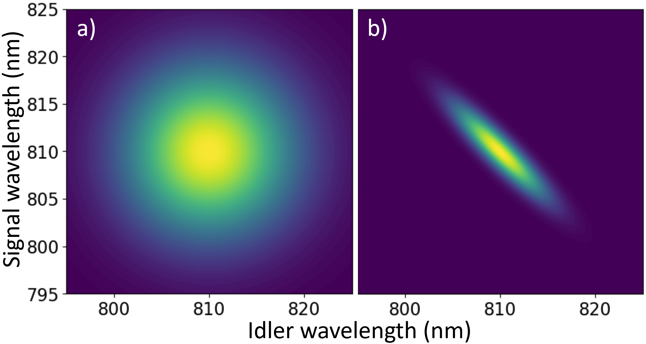
Figure 1: Joint spectral amplitudes (JSA) of two SPDC configurations, one with a) no frequency correlation and hence unit purity, and b) one with strong frequency correlation and low purity. The scale is from a high (bright green) to a low (dark purple) likelihood that the two photons exist at their respective wavelengths. For a monochromatic pump as considered in [13], the JSA would be infinitely narrow along the -45^∘ line and the purity approaches zero.

To achieve high single-photon purity $\mathcal{P}$, post-generation filtering methods are usually required to remove these correlations. Sources that attain a high $\mathcal{P}$ through strong filtering typically suffer from diminished down-converted pair production rate $\mathcal{R}$. Therefore, developing a convenient method to achieve a high $\mathcal{P}$ without sacrificing a higher $\mathcal{R}$ is desirable.

The primary purpose of this paper is to demonstrate theoretically that high single-photon purity and high two-photon heralding efficiency $\eta$ (the probability of measuring a partnered “heralded” photon upon measuring one photon) can be achieved for SPDC in bulk nonlinear optical crystals by adjusting the focal parameters of the pump beam and the down-converted collection optics. The beauty of our approach is its simplicity. We show that adjusting the Gaussian beam waists alters the transverse phase mismatch, which in turn alters the joint spectral amplitude. Because we rely on transverse phase mismatch, our approach only works for non-collinear SPDC setups, where the signal and idler modes are along different axes. This is a common method for separating signal and idler modes in bulk-crystal setups. Importantly, our approach can be applied for a wide range of pump and down-converted wavelengths in contrast to techniques that only work for a limited range of wavelengths (e.g., crystal dispersion engineering). This work will broaden the quantum toolbox for sources of entangled light.

In the next section, we discuss relevant background material such as down-converted pair source requirements, and we draw a contrast between our technique and others. In Sec. III, we discuss the various figures-of-merit that determine the quality of our proposed source. We then introduce the mechanism that allows us to tune down-conversion properties, and we show its efficacy through simulation in Sec. IV. We discuss the adjustment of other physical properties of the setup and their effects on the system in Sec. V. Section VI summarizes our findings.

II Background

In this section, we provide additional background information to set the stage for our innovation. First, we define $\eta$ as the probability of observing a photon upon observing its partner. Typically, attaining a higher $\eta$ is beneficial for entangled-photon experiments because the protocol fails if only one of the photons is received, e.g., quantum communication [6]. Many applications have a minimum required $\eta$, such as the loophole-free tests of Bell’s inequality ($\eta>66\%$ [14, 15]) and three-party quantum communication ($\eta>60\%$ [16, 17]).

Current methods of producing pure single-photons using an SPDC source can be categorized in two ways. One approach is to engineer the crystal and optics such that the down-converted photons are pure by design. In this vein, many groups rely on engineering the crystal dispersion to achieve phase matching using an auxiliary variable. For example, spectral correlations can be reduced by choosing an appropriate crystal length and pump spectral bandwidth [18]. Although this method can yield high purity ($\mathcal{P}\sim 1$), the crystal must be engineered for a specific pump wavelength, meaning there is little to no spectral flexibility [9]. Engineered material dispersion methods include introducing pulse-front-tilt on the pump beam using diffraction gratings [19]. Other groups have used apodized and chirped quasi-phase-matched periodically poled crystals [20, 21, 22, 23], or optimized aperiodically poled crystals [23, 24], etc. In general, these methods tend to be difficult and/or cumbersome.

The other approach to achieve $\mathcal{P}\sim 1$ is to use heavy spectral filtering of the down-converted pairs [25, 26]. This is a simpler approach, but it can reduce $\mathcal{P}$ because it introduces spectrally-dependent loss that affects individual photons independently [24]. Heavily filtering also greatly reduces $\mathcal{R}$, because photon pairs are removed by the filter. To counteract this loss, it is possible to multiplex heavily filtered sources, but this is also a difficult approach [27].

In contrast to these previous methods, we use a simple method that resolves the difficulties of using SPDC for producing pure single-photons while maintaining high $\eta$. Our approach does not require engineering the crystal’s dispersion, so it is applicable over a broad range of pump wavelengths. We use a hybrid technique: we loosely spectrally filter the down-converted light while adjusting the mode beam waists. This allows us to maximize $\mathcal{R}$ while maximizing $\mathcal{P}$ and $\eta$.

The relationship between $\eta$, $\mathcal{P}$, and $\mathcal{R}$ has been studied previously by Bennink [28] and Mosley et al. [9] who quantified the trade-off between $\mathcal{P}$ and $\eta$. In their works, they focused on the case of collinear SPDC, where the signal and idler modes share the same axis.

The underlying technique that we use is the same as in [28, 29]—we attempt to make the joint spectral amplitude Gaussian in signal and idler frequency space. This is done by writing the joint spectral intensity (mod-square of the JSA) in the form

$$S(\Omega_{s},\Omega_{i})=\mathcal{N}\textrm{exp}\left({-\delta_{s}\Omega_{s}^{2}-\delta_{i}\Omega_{i}^{2}-\delta_{si}\Omega_{s}\Omega_{i}}\right),$$ (1)

where $\Omega_{j}$ are the frequency detunings of the signal ($s$) and idler ($i$) photons from their phase-matched values. The spectral correlations are removed when $\delta_{si}\xrightarrow{}0$. We demonstrate the efficacy of this method in Sec. IV.

The advantage of this method is that it adds a degree-of-freedom not considered by Bennink; adjusting the focal parameters affects the degree to which the transverse phase mismatch influences the JSA. This additional degree of tunability has not been considered in the literature, and it allows us to increase both $\mathcal{P}$ and $\eta$.

In what follows, we first establish expressions for $\mathcal{R}$, $\eta$, and $\mathcal{P}$. A particular application will place a different emphasis on each metric; we investigate maximizing $\eta$ or $\mathcal{P}$ and each simultaneously. We determine the optimal values for the pump beam waist and the additional parameters such as the post-generation frequency filter width, the pump spectral bandwidth ($B_{p}$), and crystal length $L$ and cut angle (the angle between the crystal axis and the direction of pump propagation). We find that $\mathcal{P}$ and $\eta$ are tunable up to $\mathcal{P}=1$ or $\eta=1$ by adjusting the down-converted collection mode beam waists for the case when the pump beam waist sets the characteristic spatial scale, defined precisely below. Finally, we provide a detailed discussion of the trade-offs between $\eta$, $\mathcal{P}$, and $\mathcal{R}$.

III SPDC Source Figures of Merit

In SPDC, pump ($p$) photons are converted to signal ($s$) and idler ($i$) photons via a second-order nonlinear optical process described by the nonlinear polarization[30],

$$\vec{P}=\epsilon_{0}\chi^{(1)}\vec{E}+\epsilon_{0}\chi^{(2)}\vec{E}^{2}+...$$ (2)

where $\chi^{(2)}$ is the second-order susceptibility tensor responsible for SPDC as well as several other nonlinear optical phenomena such as second harmonic generation (SHG). The process of splitting photons via SPDC obeys energy conservation (a “parametric” process), where $\omega_{p}=\omega_{s}+\omega_{i}$). For peak conversion efficiency, it obeys momentum conservation ($\vec{k_{p}}=\vec{k_{s}}+\vec{k_{i}}$). Here, $\omega_{j}$ represents the angular frequency ($j$ = $p$, $s$, or $i$). Likewise, the wave vector magnitude is

$$k_{j}=\frac{n_{j}(\omega_{j})\omega_{j}}{c},$$ (3)

where the indices of refraction $n_{j}$ depend on frequency (chromatic dispersion) and polarization (birefringence) [31].

In the example below, we consider using $\beta$-barium borate (BBO), which is a negative uniaxial crystal. We then assume Type-I phase-matching, in which the pump is extraordinarily polarized and the signal and idler are both ordinarily polarized. Projecting the three modes onto ordinary and extraordinary waves, we can represent the nonzero elements of the second-order polarization in terms of the effective second-order nonlinear susceptibility, $d_{eff}$, which comprised of elements of the contracted notation nonlinear susceptibility $2d_{il}=\chi^{(2)}_{ijk}$. The terms in $d_{eff}$ are elements of the $d_{il}$ tensor that match the interaction type. For a Type-I interaction with an extraordinary pump and ordinary down-converted photons in BBO, $d_{eff}=d_{11}\cos{3\phi}\cos{\theta}-d_{31}\sin{\theta}$. Here, $\phi$ is the angle from the $x$-axis ($=0$ because there is rotational symmetry about the crystal axis in a uniaxial crystal such as BBO and we assume all modes lie in the $yz$-plane), and $\theta$ is the angle from the direction of pump propagation relative to the crystal axis (the cut angle). In our simulations below, We first determine the cut angle that produces collinear SPDC and adjust the crystal axis slightly to achieve the desired non-collinear angles of the signal and idler beams. Further explanation on our choice of cut angle is given in Sec.V.

The two-photon quantum state generated by the SPDC process is given by [24]

$$\left\lvert\psi\right\rangle=\int d\omega_{s}\int d\omega_{i}\Phi(\omega_{s},\omega_{i})\left\lvert\omega_{s}\right\rangle_{s}\left\lvert\omega_{i}\right\rangle_{i},$$ (4)

where $\left\lvert\omega_{s}\right\rangle_{s}$ and $\left\lvert\omega_{i}\right\rangle_{i}$ are the created signal and idler photon states at frequencies $\omega_{s}$ and $\omega_{i}$, respectively. The joint spectral amplitude is given by $\Phi(\omega_{s},\omega_{i})=g(\omega_{s}+\omega_{i})f(\omega_{s},\omega_{i})$, where $g(\omega_{p})$ [$f(\omega_{s},\omega_{i})$] is the pump [joint signal and idler] frequency distribution(s). The joint spectral intensity is given by $S(\omega_{s},\omega_{i})=|\Phi(\omega_{s},\omega_{i})|^{2}$.

III.1 Absolute Pair Production Rate

Our work builds on the previous work of Ling et al. [32] and Guilbert et al. [13], who considered the SPDC process pumped by a monochromatic laser, and the work of Valencia et al. [29], who consider a pulsed laser source with pulse-front tilt. The studies using monochromatic pump light adjusted the pump beam and collection beam waists to obtain $\eta\sim 1$, but monochromatic pumping gives rise to frequency correlations such as that shown in Fig. 1a. The study considering pulsed pump light adjusted the pump beam and collection mode waists and pulse front tilt to obtain $\mathcal{P}\sim 1$, but they did not attempt to optimize $\eta$ or $\mathcal{R}$. Here, we combine both theoretical approaches to answer whether all three metrics can be optimized simultaneously.

To begin, we introduce Hermite-Gauss mode functions given by

$$U_{n,m}(x,y,z)=\alpha^{(n,m)}G_{n}\left(\frac{\sqrt{2}x}{W(z)}\right)G_{m}\left(\frac{\sqrt{2}y}{W(z)}\right)\\ \times\textrm{exp}\left(-ikz-ik\frac{x^{2}+y^{2}}{2R(z)}+i(m+n+1)\zeta\right).$$ (5)

where

$$\alpha^{(n,m)}=\sqrt{\frac{2}{2^{n+m}n!m!\pi W_{0}^{2}}},$$ (6)

$$G_{n}(u)=H_{n}(u)\textrm{exp}\left(-\frac{u^{2}}{2}\right),$$ (7)

$H_{n}(u)$ is a Hermite polynomial, and $W(z)$ is the $z$-dependent beam radius in the nonlinear crystal, defined as the $1/e$ field radius. We consider all modes to lie in the $yz$-plane, so while $x$ is the same for all modes, $y$ and $z$ are different for each ($z$ being that mode’s propagation direction). The minimum beam radius $W_{0}$ (the ‘beam waist’) is related to the Rayleigh range through the relation $z_{r}=\pi W_{0}^{2}/\lambda$, where $\lambda$ is the vacuum wavelength. We assume that the beam waists for all three modes are at the center of the crystal so that the waist for other positions is given by $W(z)=W_{0}\sqrt{1+(z/z_{r})^{2}}$.

We focus on the case where $z_{r}\gg L$, appropriate for thin crystals often used when pumping with short-pulse laser light needed to obtain high $\mathcal{P}$. Under this assumption, we can take $k(x^{2}+y^{2})/R\sim 0$ and the Guoy phase $\zeta\sim 0$, which greatly simplifies evaluating the integral in Eq. (4). Working in the thin-crystal regime also allows us to consider the beam radii to be at their minima throughout the length of the crystal, such that for the $j$-mode (where $j=s\textrm{, }i\textrm{, or }p$), $W_{j}(z)=W_{0,j}$.

The geometry of the fundamental Gaussian modes of the pump beam and the collecting optics are shown in Fig. 2. The emission angle $\theta_{s}$ ($\theta_{i}$) for the signal (idler) beam is greatly exaggerated for illustrative purposes. We consider emission angles so small that all modes essentially overlap in the crystal. The crystal cut angle is not shown to keep the figure simple; the crystal axis differs from the $z$-axis by the cut angle for the uniaxial crystal considered here.

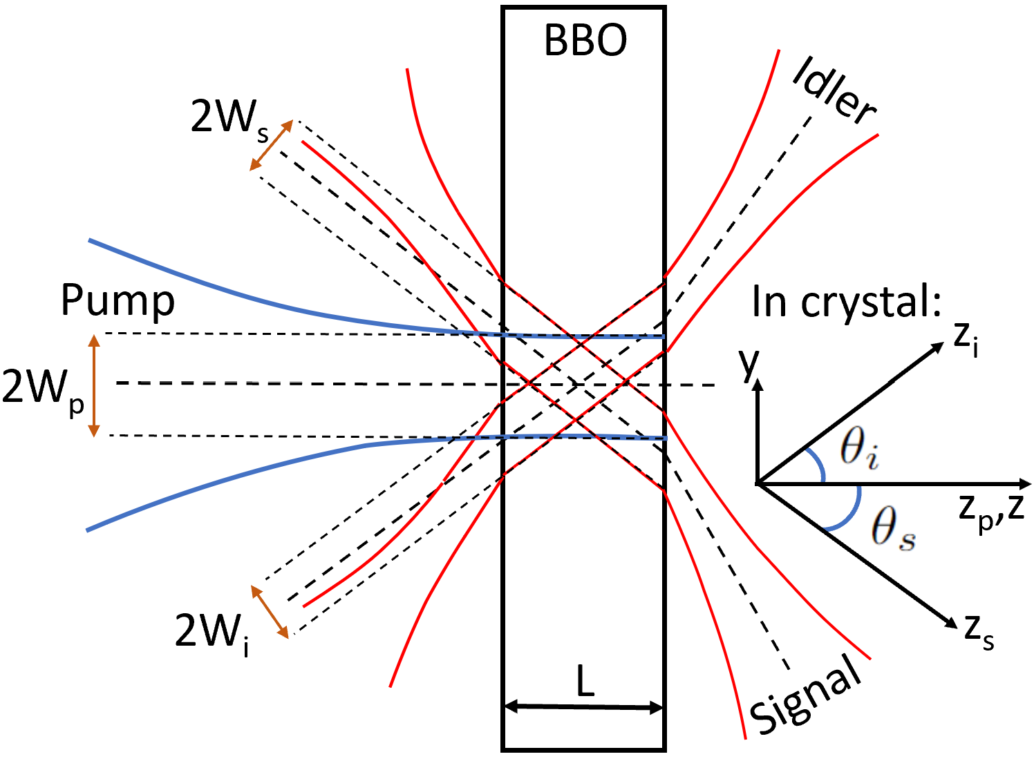
Figure 2: Geometry of the SPDC interaction. The focal conditions of the pump (blue lines indicate $1/e$ field radius of pump), signal, and idler beams (red lines indicate $1/e$ field radius of signal and idler). The beam waist radii are $W_{0,p}$, $W_{0,s}$, $W_{0,i}$. The beams are aligned such that the three modes overlap as much as possible inside the crystal (perfect intersection at the center ($L$/2) of the crystal).

Using this definition for the mode function, the joint spectral amplitude is given by [13],

$$\Phi(\omega_{s},\omega_{i})=g(\omega_{s}+\omega_{i})\times\\ \int_{L/2}^{L/2}dz\int_{-\infty}^{\infty}\int_{-\infty}^{\infty}dxdyU_{p}(x,y)U_{s}(x,y)U_{i}(x,y)\\ \times\textrm{exp}\left\{i\left[k_{p}z-k_{s}(-\sin\theta_{s}y+\cos\theta_{s}z)\right.\right.\\ \left.\left.-k_{i}(-\sin\theta_{i}y+\cos\theta_{i}z)\right]\right\},$$ (8)

The inclusion of the pump spectral distribution $g(\omega_{s}+\omega_{i})$ is where our theory differs from Ling et al. and Guilbert et al., where they take $a$ to be a flat distribution. We consider a Gaussian pump distribution

$$g(\omega_{s}+\omega_{i})=\textrm{exp}\left(-\frac{(\omega_{s}+\omega_{i}-\omega_{p0})^{2}}{4B_{p}^{2}}\right),$$ (9)

where $B_{p}$ is the pump beam spectral bandwidth, $\omega_{p0}$ is the central frequency of the pump.

The frequency dependence of $\Phi(\omega_{i},\omega_{s})$ arises from the frequency dependence of $k_{j}$, given in Eq. (3). The complex exponential in Eq. (8) was extracted from Eq. (5) after our approximations, while the rest of Eq. (5) remains in each $U_{j}(x,y)$. The factor that multiplies each mode’s wave number ($k_{j}$ for $j=p,\textrm{ }s,\textrm{ and }i$) is that mode’s propagation direction.

We rewrite this complex exponential more compactly in terms of the phase mismatch $\vec{\Delta k}$. This quantifies momentum conservation for a specific combination of frequencies and indices of refraction.

In the calculation of the pair production rate, we consider all three field modes to be in the fundamental (Gaussian) mode, so that we may write

$$\Phi(\omega_{s},\omega_{i})=g(\omega_{s}+\omega_{i})\int dz\int dxdye^{i\vec{\Delta k}\textrm{ }\vec{r}}\\ \times\textrm{exp}\left(\frac{-(x^{2}+y^{2})}{W_{0,p}^{2}}\right)\\ \times\textrm{exp}\left(\frac{-(x^{2}+(y\cos{\theta_{s}}+z\sin{\theta_{s}})^{2})}{W_{0,s}^{2}}\right)\\ \times\textrm{exp}\left(\frac{-(x^{2}+(y\cos{\theta_{i}}-z\sin{\theta_{i}})^{2})}{W_{0,i}^{2}}\right),$$ (10)

where each term is a Gaussian function in that mode’s transverse spatial dimension. We consider the fundamental modes because that is by far the most likely mode for signal and idler to occupy simultaneously when coupling the light into single mode fiber. When we consider signal and idler singles rates we use the full version of $U_{j}(x,y)$ from Eq. (5). This will help determine the fraction of signal and idler photons that remain within the fundamental mode compared to those that escape to higher-order Hermite-Gauss modes (the heralding efficiency).

In non-collinear setups like ours, $\vec{\Delta k}$ is typically split into transverse ($\Delta k_{y}$) and longitudinal ($\Delta k_{z}$) components given by

$$\Delta k_{y}=k_{s}\sin\theta_{s}-k_{i}\sin\theta_{i},$$ (11)

and

$$\Delta k_{z}=k_{p}-k_{s}\cos\theta_{s}-k_{i}\cos\theta_{i}.$$ (12)

The integration over the $x$- and $y$-variables is straightforward and gives us

$$\Phi(\omega_{s},\omega_{i})=g(\omega_{s},\omega_{i})\frac{\pi}{\sqrt{AC}}\textrm{exp}\left(-\frac{\Delta k_{y}^{2}}{4C}\right)\\ \times\int^{L/2}_{-L/2}\textrm{exp}(-Hz^{2}-i\Delta k_{z}z),$$ (13)

where

$$A=\frac{1}{W_{0,p}^{2}}+\frac{1}{W_{0,s}^{2}}+\frac{1}{W_{0,i}^{2}},$$ (14)

$$C=\frac{1}{W_{0,p}^{2}}+\frac{\cos^{2}\theta_{s}}{W_{0,s}^{2}}+\frac{\cos^{2}\theta_{i}}{W_{0,i}^{2}}.$$ (15)

$$D=\frac{\sin 2\theta_{s}}{W_{0,s}^{2}}-\frac{\sin 2\theta_{i}}{W_{0,i}^{2}}$$ (16)

$$F=\frac{\sin^{2}\theta_{s}}{W_{0,s}^{2}}+\frac{\sin^{2}\theta_{i}}{W_{0,i}^{2}}$$ (17)

$$H=F-\frac{D^{2}}{4C}$$ (18)

The effect of spatial walk-off (the difference in phase propagation direction and the direction of energy flow) is given in the spatial integral in the $z$-direction in Eq. (13) [32]

$$\Phi_{z}=\int^{L/2}_{-L/2}dz\textrm{ exp}(-Hz^{2}-i\Delta k_{z}z).$$ (19)

Considering small angles $\theta_{s}$ and $\theta_{i}$ and a thin crystal, the walk-off factor ($H$) is approximately zero, and thus we ignore the spatial walk-off. This approximation greatly speeds up computation time and only results in a $\approx 1\%$ error in $\eta$. The result is

$$\Phi(\omega_{s},\omega_{i})=\frac{\pi L}{\sqrt{AC}}\textrm{sinc}\left(\Delta k_{z}L/2\right)\\ \times\textrm{exp}\left(-\frac{\Delta k_{y}^{2}}{4C}-\frac{(\omega_{s}+\omega_{i}-\omega_{p0})^{2}}{4B_{p}^{2}}\right).$$ (20)

Our goal is to express the joint spectral intensity in the form of Eq. (1). Therefore, we write the components of the mode function in terms of frequency detuning from the central frequency (the one that yields phase matching at the central pump frequency). Starting with the wave vector magnitudes, we write them as a first-order Taylor expansion about each mode’s central frequency as

$$k_{j}=k_{j0}+N_{j}\Omega_{j},$$ (21)

where we introduce the inverse group velocity $N_{j}=(dk_{j}/d\omega_{j})_{\omega_{j0}}$ [29]. Here, $\Omega_{j}=\omega_{j}-\omega_{j0}$ is the frequency detuning of mode $j$. Using Eq. (21) in Eq. (11) and Eq. (12), the zero-order terms drop out and we are left with

$$\Delta k_{y}=N_{s}\Omega_{s}\sin\theta_{s}-N_{i}\Omega_{i}\sin\theta_{i},$$ (22)

and

$$\Delta k_{z}=N_{p}\Omega_{p}-N_{s}\Omega_{s}\cos\theta_{s}-N_{i}\Omega_{i}\cos\theta_{i}.$$ (23)

We also write the pump spectral distribution from Eq. (9) in terms of the signal and idler frequency detunings,

$$g(\Omega_{s},\Omega_{i})=\frac{(\Omega_{s}+\Omega_{i})^{2}}{4B_{p}^{2}}.$$ (24)

Writing everything involved in the mode function in terms of frequency detuning is useful because a frequency uncorrelated JSA (as in Fig. 1a, a pure source) should be a Gaussian function of signal and idler frequency detuning. The result is

$$\Phi(\Omega_{s},\Omega_{i})=\frac{\pi L}{\sqrt{AC}}\textrm{sinc}\left(\Delta k_{z}L/2\right)\\ \times\textrm{exp}\left(-\frac{\Delta k_{y}^{2}}{4C}-\frac{(\Omega_{s}+\Omega_{i})^{2}}{4B_{p}^{2}}\right),$$ (25)

where the phase mismatches are given in equations (22) and (23).

After collecting constants used in previous derivations [13, 32], the emission rate is calculated numerically using

$$\mathcal{R}=\frac{\eta_{s}\eta_{i}Pd_{eff}^{2}\alpha_{s}^{2}\alpha_{i}^{2}\alpha_{p}^{2}\omega_{s}\omega_{i}}{\sqrt{2}\pi^{3/2}\epsilon_{0}c^{3}n_{s}n_{i}n_{p}B_{p}}\int_{-\infty}^{\infty}\int_{-\infty}^{\infty}T_{s}(\omega_{s})\\ \times T_{i}(\omega_{p}-\omega_{s})|\Phi(\Omega_{s},\Omega_{i})|^{2}d\omega_{s}d\omega_{p},$$ (26)

which yields the pair rate in units of pairs/s. Here, $\eta_{j}$ are the overall signal/idler path efficiencies, and

$$\alpha_{j}=\sqrt{\frac{2}{\pi W_{0,j}^{2}}},$$ (27)

are the fundamental mode normalization constants [$\alpha^{(0,0)}$ in Eq. (6)], $\epsilon_{0}$ is the vacuum permittivity constant, and the filter transmission functions (which in this paper we consider to be ideal unit efficiency bandpass filters) are $T_{j}$. Dividing through by the pump power $P$ in milliwatts (mW) gives us the absolute pair emission rate in the useful units of $[\mathcal{R}]=$ pairs/(s mW), seeing that the rate scales linearly with pump power.

In the expression for the biphoton mode function Eq. (20), the factor that involves the beam waists parameter ($C$) is the foundation of our purity maximization technique. By changing the beam waists in $C$, we change the dependence of the spectrum on the transverse phase mismatch. Therefore, the new technique we introduce is only applicable to noncollinear setups. Otherwise, $\Delta k_{y}=0$ and the frequency-dependent portion of $\Phi(\Delta k)$ is independent of beam waists. The constants in the form of $1/\sqrt{AC}$ remain, but they do not influence frequency dependence. In Sec. IV we expand this idea. There, we first massage the mod-square of Eq. (20) into the form of Eq. (1). This immediately leads to a purity maximization condition ($\delta_{si}\xrightarrow{}0$), which we then explore the details of.

III.2 Heralding Efficiency

The heralding efficiency is given by

$$\eta=\frac{\mathcal{R}}{\sqrt{\mathcal{R}_{s}\mathcal{R}_{i}}},$$ (28)

where the $\mathcal{R}_{s(i)}$ is the rate of signal (idler) single-photon production rate and $\mathcal{R}$ is the joint count rate.

The singles spectrum and rate are derived in a similar manner as the joint spectrum and joint rate above. The difference is that when calculating the signal (idler) singles spectrum, we need to consider the higher-order non-Gaussian modes that the signal (idler) can escape to.

We take a summation over all modes $(n,m)$ given in Eq. (5) and get the signal (idler) singles rate given by

$$\mathcal{R}_{s(i)}=\sum\limits_{n,m=0}^{\infty}\frac{\eta_{s(i)}Pd_{eff}^{2}(\alpha_{s(i)}^{(n,m)})^{2}\alpha_{i(s)}^{2}\alpha_{p}^{2}\omega_{s}\omega_{i}}{\sqrt{2}\pi^{3/2}\epsilon_{0}c^{3}n_{s}n_{i}n_{p}B_{p}}\\ \times\int_{-\infty}^{\infty}\int_{-\infty}^{\infty}T_{s(i)}(\omega_{s(i)})|\Phi_{s(i)}^{(n,m)}(\Omega_{s},\Omega_{i})|^{2}\\ \times d\omega_{s(i)}d\omega_{p}.$$ (29)

In Eq. (29), the shape of the pump spectrum is included in $\Phi_{s(i)}^{(n,m)}$, which is the mode function for a given (n,m). From here, $\eta$ is calculated by using both Eq. (26) and Eq. (29) in Eq. (28).

III.3 State Purity

The biphoton state purity is determined by the spectral factorability of the joint spectrum into two separate photon states. In general, the wave function can be expressed using Schmidt decomposition as [9]

$$\Phi(\omega_{s},\omega_{i})=\sum\limits_{n}\sqrt{\lambda_{n}}\phi_{n}(\omega_{s})\psi_{n}(\omega_{i}),\hskip 8.5359pt\sum\limits_{n}\lambda_{n}=1,$$ (30)

where $\phi_{n}(\omega_{s})$ and $\psi_{n}(\omega_{i})$ are orthogonal modes in frequency space. Each combination of modes has a weight $c_{n}$, from which we obtain the state purity,

$$\mathcal{P}=\sum\limits_{n}\lambda_{n}^{2},$$ (31)

the inverse of which is the Schmidt number.

However, for the general case, Schmidt decomposition is not always analytically possible. Therefore, we use the equivalent numerical method, singular value decomposition. We calculate a representative set of joint spectral amplitudes for combinations $(\omega_{s},\omega_{i})$ within the range of our spectral filtering. These values correspond to an $n\times m$ matrix of values $\left|\Phi(\omega_{s_{n}},\omega_{i_{m}})\right|^{2}$ which we then perform singular value decomposition. In analogy to Eq. (31), the sum of the squared singular values of the joint spectral amplitude matrix is treated as the spectral purity.

IV Tuning the Properties of Generated Photon Pairs

IV.1 Methodology

Previously, methods of tuning the properties of down-converted photon pairs were often difficult to use, and at best inconvenient. Our proposed technique draws from the findings of previous authors and pulls them together. First, we use the important approximation that Valencia et al. [29] use that allows us to write the phase matching sinc function as an exponential that has the same width at $1/e^{2}$ of the intensity ($1/e$ of the field amplitude),

$$\text{sinc}(x)=e^{-\alpha x^{2}},$$ (32)

where the constant $\alpha=0.455$. Equation (32) can be used to represent the joint spectral amplitude of the biphoton (the modulus square of the mode function, Eq. (20) above) as

$$S(\Omega_{s},\Omega_{i})=\mathcal{N}\times\\ \textrm{exp}\left(-\frac{\Delta k_{y}^{2}}{2C}-\alpha\Delta k_{z}L-\frac{(\Omega_{s}+\Omega_{i})^{2}}{2B_{p}^{2}}\right).$$ (33)

The more general form, written in terms of the three fields’ frequency detunings, is shown in Eq. (1). Using the expressions for $\Delta k_{y}$ and $\Delta k_{z}$ above [Eq. (11) and Eq. (12), respectively], we have

$$\delta_{s}=\frac{N_{s}^{2}\text{sin}^{2}\theta_{s}}{4C}+\frac{\alpha^{2}(N_{p}-N_{s}\text{cos}\theta_{s})^{2}L^{2}}{4}+\frac{1}{4B_{p}^{2}},$$ (34)

$$\delta_{i}=\frac{N_{i}^{2}\text{sin}^{2}\theta_{i}}{4C}+\frac{\alpha^{2}(N_{p}-N_{i}\text{cos}\theta_{i})^{2}L^{2}}{4}+\frac{1}{4B_{p}^{2}},$$ (35)

and

$$\begin{split}\delta_{si}=-\frac{\alpha^{2}(N_{p}-N_{s}\text{cos}\theta_{s})(N_{p}-N_{i}\text{cos}\theta_{i})L^{2}}{2}\\ +\frac{1}{2B_{p}^{2}}-\frac{N_{s}\text{sin}\theta_{s}N_{i}\text{sin}\theta_{i}}{2C}.\end{split}$$ (36)

By setting $\delta_{si}=0$, we ensure the signal and idler are separable in frequency and therefore spectrally indistinguishable. One may think of this as a JSA that has an elliptical shape with major and minor axes along $\Omega_{s}$ and $\Omega_{i}$ such that no general correlations exist between signal and idler frequencies. The easiest version of this to imagine is that where the major and minor axes are equal, resulting in a three-dimensional Gaussian spectrum, seen in Fig. 1a.

When we use $C$ from Eq. (15) in Eq. (36) for the noncollinear case (and set $W_{0,i}=W_{0,s}$), the purity condition Eq. (36) becomes a relationship between Gaussian mode beam waists $W_{0,s}$ and $W_{0,p}$

$$W_{0,s}=(\text{cos}^{2}\theta_{s}+\text{cos}^{2}\theta_{i})^{\frac{1}{2}}\\ \times\bigg{(}\frac{N_{i}N_{s}\text{sin}\theta_{i}\text{sin}\theta_{s}}{\frac{1}{B_{p}^{2}}+\alpha^{2}L^{2}(N_{p}-N_{i}\text{cos}\theta_{i})(N_{p}-N_{s}\text{cos}\theta_{s})}\\ -\frac{1}{W_{0,p}^{2}}\bigg{)}^{-\frac{1}{2}}.$$ (37)

Setting the down-converted collection mode beam waists equal is useful for both maximizing the photon pair rate [13, 32], and for greatly simplifying the form of Eq. (37). Using the approximation we introduced for $W(z)$ in Eq. (5) in Sec. III, we rationalize why the two beam waists may be taken as equal (even in the non-degenerate case). The difference in wavelength between the two down-converted modes in the non-degenerate case technically results in a difference in spot size evolution, according to our definition of $W_{j}(z)$. We consider this negligible for large $z_{r,j}$ and a thin crystal, just as we assume $W_{j}(z)\approx W_{0,j}$ in the crystal.

The purity condition Eq. (37), the result of requiring $\delta_{si}=0$, can only be achieved for certain combinations of values. For example, at $\theta_{j}=0$ (collinear setups), the term involving $C$ is zero. Alterations of the beam waists then have a less pronounced effect on $\mathcal{P}$—while $\mathcal{P}$ is still affected by changing beam waists, they are no longer a part of the purity condition. Equation (36) then yields a fixed relationship between $B_{p}$ and $L$ (where they are inversely proportional). Although it is still possible to reach high $\mathcal{P}$ using this relationship, it is without the additional degree-of-freedom from the beam waists. Thus, better combinations of $\eta$, $\mathcal{P}$, and $\mathcal{R}$ are sacrificed when using the collinear case. Bennink [28] discusses the collinear case, including how changing Gaussian beam waists affect $\mathcal{P}$ and $\eta$.

We first iteratively maximize our figures of merit in these variables (as well as cut angle, filter widths, etc.). We then tune the beam waists, something not considered for noncollinear setups in the past which should allow $\mathcal{P}=1$.

To maximize the $\eta$, $\mathcal{P}$, and $\mathcal{R}$, we first iterate over values of $W_{0,p}$ to maximize $\mathcal{R}$. We use this value of $W_{0,p}$ in the purity condition [Eq. (37)] to find the corresponding $W_{0,s}$. Then, we detune $W_{0,s}$ and find, through simulation, the value of $W_{0,s}$ that results in the highest $\mathcal{P}$ [in our setup, Eq. (37) tends to overestimate the ideal value of $W_{0,s}$]. These steps are repeated many times using different values for the different constants of the system (such as cut angle, filter widths, crystal length, etc.). This requires many trade-offs between the figures-of-merit that each researcher using this model can choose depending on what they value the most for a given application. Many such relationships will be explored in Sec. V. The constants we choose yield good $\mathcal{R}$, and the highest values of $\eta$ possible while still achieving unit $\mathcal{P}$.

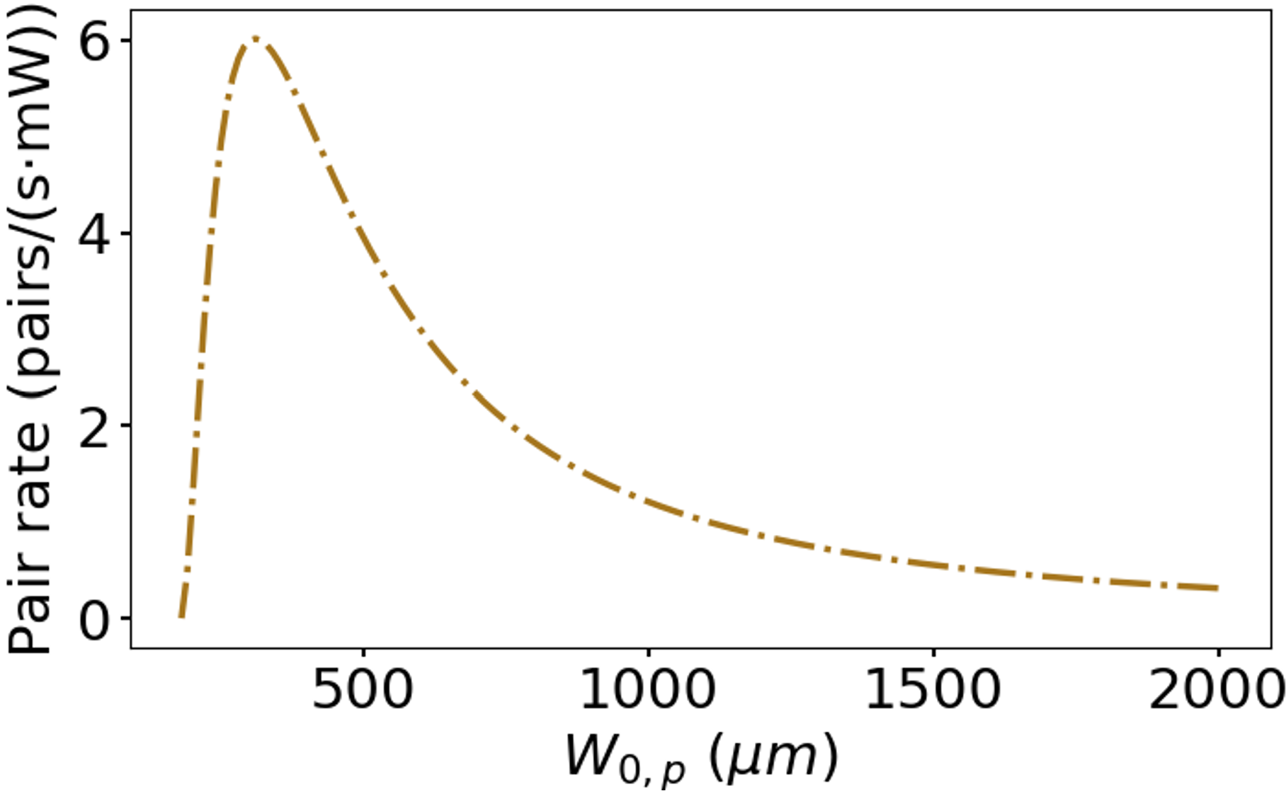
Figure 3: The pair production rate as a function of the pump beam waist.

Using this technique, the ideal values of these constants for our setup include a BBO crystal length of $450\textrm{ }\mu m$; a crystal cut angle detuning (angular perturbation from the cut angle that produces collinear signal and idler beams) of $1.5^{\circ}$; a flat-top unit efficiency spectral filter on the down-converted beam with a half-width of $5\textrm{ THz}$ ($\Delta\omega_{s}=\Delta\omega_{i}=10\textrm{ THz}$, Fig. 5); a spectral filter on the pump beam twice as wide as that used on the down-converted beams; and a pump bandwidth of $30\textrm{ THz}$.

IV.2 Non-collinear Degenerate.

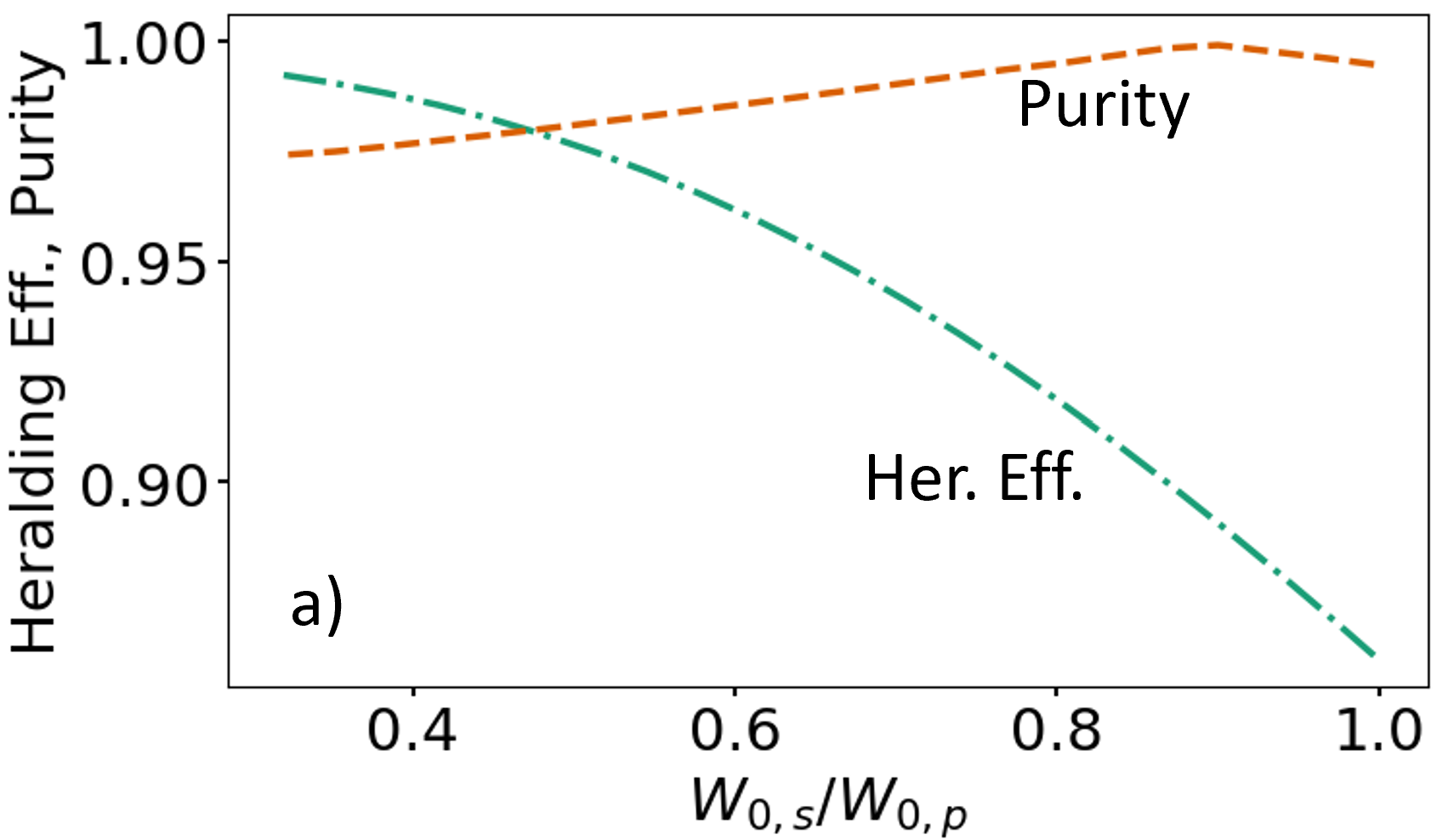
Figure 4: Non-Collinear Degenerate. a) Heralding efficiency and biphoton state purity as a function of $W_{0,s}/W_{0,p}$. b) Pair production rate as a function of $W_{0,s}/W_{0,p}$.

Non-collinear setups are achieved by altering the crystal’s cut angle. Collinear setups require a specific cut angle unless non-critical phase matching is used (crystal axis and pump propagation direction are orthogonal). For a non-collinear geometry, we consider a small $1.5^{\circ}$ detuning from the collinear cut angle (determined iteratively as discussed in Sec. IV). Our calculations assume a nearly complete overlap between the pump and down-converted beam collection modes, which is still valid for our choice of cut angle and crystal length. Others [13] have considered setups that have approximately a $\approx 3^{\circ}$ full angle between signal and idler outside the crystal, but we see no reason to sacrifice $\mathcal{P}$ through limiting transverse phase mismatch when pump beam spatial walk-off is affected in such a minor way. In the degenerate case, we assume the signal and idler pairs are created around 810 nm. As shown in Fig. 3, the maximum $\mathcal{R}$ occurs at a pump beam waist of $W_{0,p}=310\textrm{ }\mu m$. Using the purity maximizing condition Eq. (37), we find $W_{0,s}$ given this $W_{0,p}$. Then, we detune $W_{0,s}$ to see how our figures of merit change as a function of $W_{0,s}$ in Fig. 4 (where the horizontal axis the ratio of $W_{0,s}$ to the ideal rate-maximizing $W_{0,p}$).

In Fig. 4a we see that the intersection of $\mathcal{P}=\eta=0.98$ occurs at $145.4\textrm{ }\mu$m, corresponding to $W_{0,s}/W_{0,p}=0.469$. Altering the setup to achieve $\mathcal{P}\approx 1$ only requires adjusting $W_{0,s}$ to $280\textrm{ }\mu$m, which corresponds to $W_{0,s}/W_{0,p}\approx 0.90$. This technique is therefore not only versatile but also strong.

IV.3 Non-collinear Non-degenerate.

A non-degenerate SPDC source is also sometimes referred to as “bichromatic.” To keep $\eta$ as high as possible, the filters are equidistant on either side of half the central pump frequency (energy conservation dictates down-converted pair symmetry about the degenerate frequency), as shown in Fig. 5. These bands of light sometimes overlap and can be separated using spectral filtering, but that is unnecessary here due to the non-collinear geometry. The wavelength and bandwidth of the pump remain the same as in our degenerate setup. We chose the central signal wavelength to be 850 nm and the corresponding energy-conserving central wavelength of the idler is 609.6 nm. As in the degenerate case, $W_{0,p}\approx 310\textrm{ }\mu m$ maximizes $\mathcal{R}$ (the plot looks nearly identical to Fig. 3, so we do not include it here). Using the purity condition Eq. (37) to calculate $W_{0,s}$ given $W_{0,p}$, we look at the relationships between $W_{0,s}/W_{0,p}$ (where we use $W_{0.p}=310\textrm{ }\mu$m) and our figures of merit in Fig. 6.

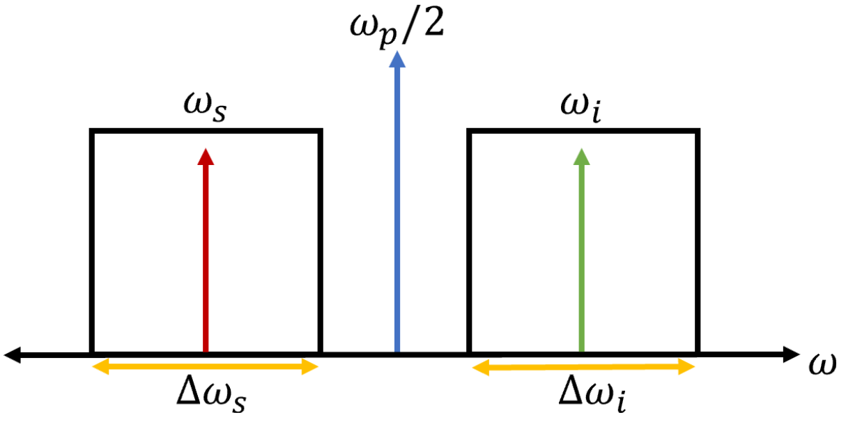
Figure 5: The unit efficiency bandpass filters considered for the non-degenerate case. They are spaced evenly about the degenerate frequency ($\omega_{p}$) and $\Delta\omega_{s(i)}=10\textrm{ THz}$.

Equation (37) is based on approximation in Eq. (32), so it does not guarantee unit $\mathcal{P}$. The largest values on the horizontal axes in Figs. 4 (corresponding to $W_{0,s}=309\textrm{ }\mu\textrm{m}$) and  6 (corresponding to $W_{0,s}=305.4\textrm{ }\mu\textrm{m}$) are those that Eq. (37) predicts will yield unit $\mathcal{P}$. In both the degenerate and nondegenerate cases, unit $\mathcal{P}$ is achieved at $W_{0,s}/W_{0,p}\approx 0.90$, which corresponds to $W_{0,s}\approx 280\textrm{ }\mu\textrm{m}$, approximately $10\%$ off of what Eq. (37) predicts. Using Eq. (32) is therefore not practical for obtaining exact results; however, it is a useful tool to get close to unit $\mathcal{P}$. When used in conjunction with our simulation, detuning the down-converted beam waists then brings the setup to unit $\mathcal{P}$.

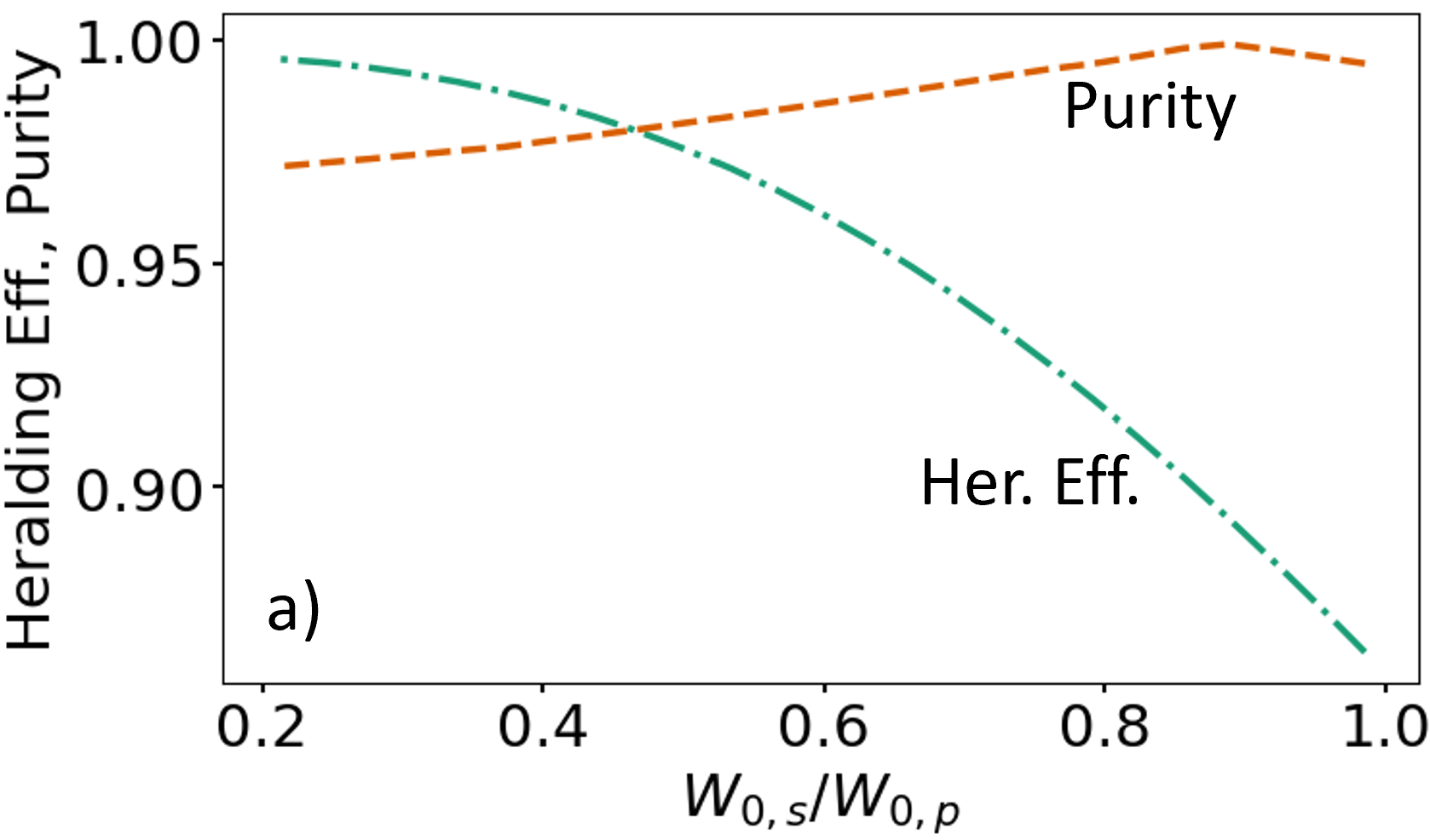
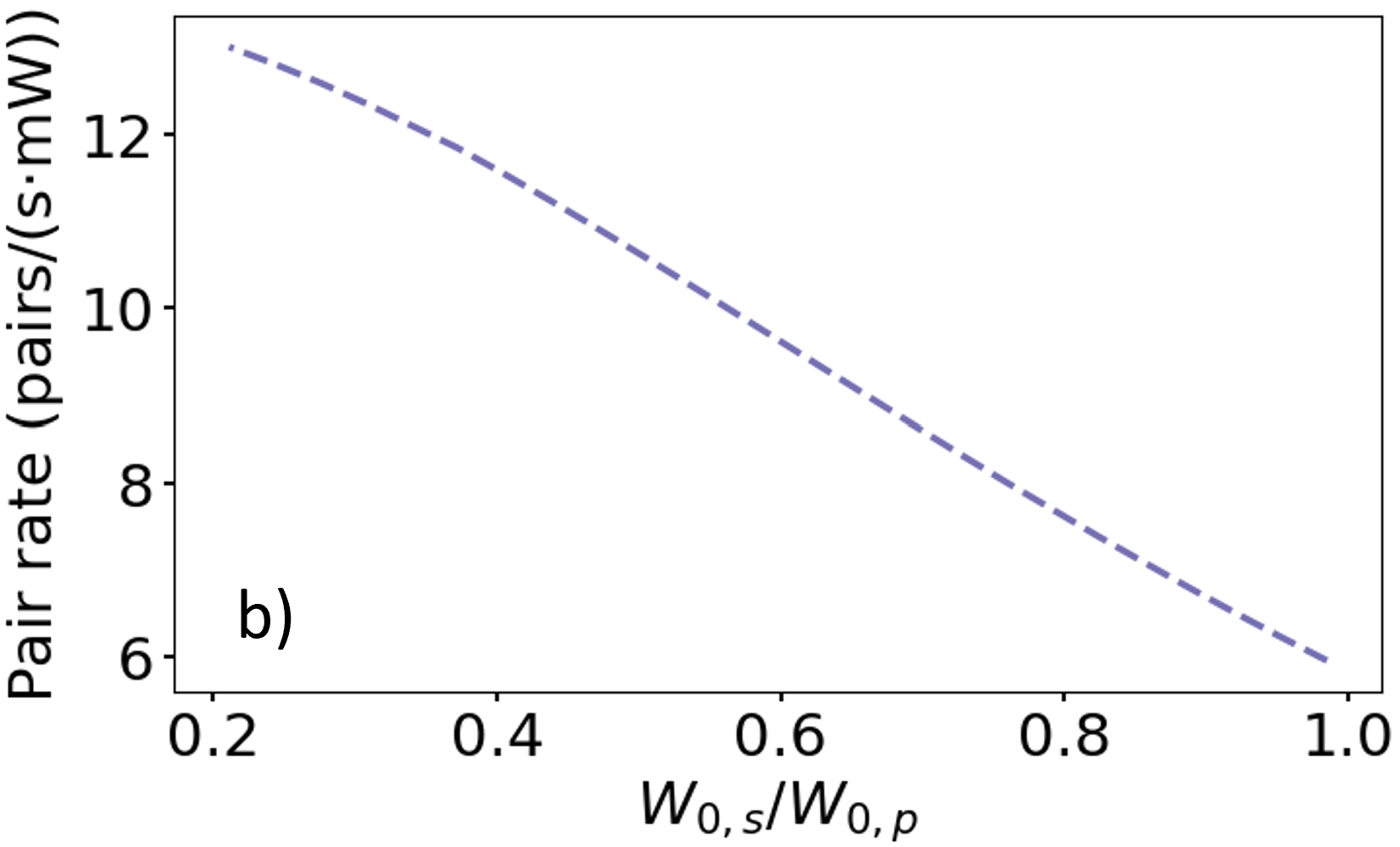
Figure 6: Non-Collinear Non-Degenerate. a) Heralding efficiency and biphoton spectral purity as a function of $W_{0,s}/W_{0,p}$. b) Pair production rate as a function of $W_{0,s}/W_{0,p}$.

V Generalization to other variables

Although we mainly focused on the relationship between the down-converted/pump beam waists and the figures of merit, there are trade-offs to explore in the alteration of the constants appearing in Eq. (26), (29), and (36). The most straightforward way to understand their effect on $\mathcal{P}$ is to think of how well $\delta_{si}=0$ can be enforced for a given set of variables. Parameters that are in the singles and pair production rate [Eq. (29) and (26), respectively] have an effect on $\eta$, as seen in Eq. (28). Naturally, the parameters changing in the equation for $\mathcal{R}$ Eq. (26) will affect it.

Increasing the down-converted frequency filter widths decreases $\mathcal{P}$ and $\eta$ while increasing the rate. The primary purpose of the down-converted beam filters is to eliminate any remaining frequency correlations in the region of large $\Omega_{s}$ and $\Omega_{i}$, increasing $\mathcal{P}$. However, strong filtering (decreasing filter widths) significantly lowers $\mathcal{R}$, as mentioned in Sec. II.

As the cut angle detuning increases (decreases), the angle between the two down-converted beams increases (decreases). The cut angle must be large enough to introduce a transverse phase mismatch that can be tuned by adjusting the beam waists, using our purity condition Eq. (37). At small values of $\theta_{j}$ (for $j=s,i$), Eq. (37) can only be satisfied for large pump spectral bandwidths.

Looking beyond experimental logistics, an increase in pump spectral bandwidth decreases $\mathcal{R}$. A larger cut angle will introduce a more substantial Poynting vector walk-off. This will make our approximation of negligible walk-off between Eq. (19) and Eq. (20) inaccurate. Generally, greater walk-off will negatively impact $\eta$ and $\mathcal{R}$ due to less beam overlap inside the crystal (thus, the issue also worsens with greater crystal length).

In tuning the cut angle, it is also important to remember that one is also altering $d_{eff}$, the refractive indices, and the phase mismatch. We considered a cut angle detuning of $1.5^{\circ}$ (which produces a full external angle of $\approx 12^{\circ}$ between signal and idler beams), which results in the walk-off angle of the pump beam only growing by $0.078^{\circ}$ (or $1.83\%$ of the collinear pump walk-off, which occurs for a $4.21^{\circ}$ cut angle). We have found, through simulation, that including the walk-off term only results in a $\approx 0.3\%$ difference in the overall joint count rate. This indicates that, for our chosen value of crystal cut angle, the spatial walk-off has a negligible effect on the system. In contrast, a larger cut angle will have a more dramatic negative effect.

For an increasing crystal length, $\mathcal{R}$ rises and falls as expected for an imperfectly phase-matched SPDC setup [30]. The heralding efficiency, however, decreases with greater crystal length. This is because the purity condition [Eq. (37)] will require a larger $W_{0,s}$, which leads to a lower $\mathcal{R}$ and a lower $\eta$ (in agreeance with [13]). A longer crystal also means less beam spatial overlap in the crystal, eventually making our approximation of Eq. (19) for negligible walk-off inaccurate.

The trade-offs in altering the physical parameters of the system make it convenient to choose values for each that approximately optimize the system (according to simulation) and then tune the Gaussian beam waists for fine control over the figures of merit. This is the technique we used in our simulation, which we used to produce Figs. 3, 4, and 6 above (as well as the optimal values of $\eta$ and $\mathcal{P}$ that we claim are possible).

VI Conclusions

We show that it is possible to achieve tunable heralding efficiency and purity in an SPDC setup by changing only the beam focal parameters. This technique will enable researchers to produce a pure single-photon source using basic optical equipment and a bulk nonlinear crystal, once initial parameters such as crystal length are chosen. Our model enables us to predict that, for both non-collinear degenerate and non-degenerate setups at unit purity, the heralding efficiency can be as high as $\approx 0.90$, and purity and heralding efficiency intersect at $\approx 0.98$. Our setup is therefore a cost-effective way to bypass more expensive or complicated setups with theoretically comparable results. We remove the need to specially engineer crystals and waveguides for purity or heralding efficiency and also eliminate the need to strongly filter the down-converted beams (increasing pair production rate). Additionally, our setup can operate over a broad range of pump wavelengths, unlike crystal dispersion-engineered pure single photon sources.

References

- Ren et al. [2017] J.-G. Ren, P. Xu, H.-L. Yong, L. Zhang, S.-K. Liao, J. Yin, W.-Y. Liu, W.-Q. Cai, M. Yang, L. Li, et al., Ground-to-satellite quantum teleportation, Nature 549, 70 (2017).
- Shen et al. [2023] S. Shen, C. Yuan, Z. Zhang, H. Yu, R. Zhang, C. Yang, H. Li, Z. Wang, Y. Wang, G. Deng, et al., Hertz-rate metropolitan quantum teleportation, Light Sci. Appl. 12, 115 (2023).
- Couteau [2018] C. Couteau, Spontaneous parametric down-conversion, Contemp. Phys. 59, 291 (2018).
- Kwiat et al. [1995] P. G. Kwiat, K. Mattle, H. Weinfurter, A. Zeilinger, A. V. Sergienko, and Y. Shih, New high-intensity source of polarization-entangled photon pairs, Phys. Rev. Lett. 75, 4337 (1995).
- Kwiat et al. [1993] P. G. Kwiat, A. M. Steinberg, and R. Y. Chiao, High-visibility interference in a bell-inequality experiment for energy and time, Phys. Rev. A 47, R2472 (1993).
- Piveteau et al. [2022] A. Piveteau, J. Pauwels, E. Håkansson, M. Bourennane, and A. Tavakoli, Entanglement-assisted quantum communication with simple measurements, Nat. Comm. 13, 7878 (2022).
- Boaron et al. [2018] A. Boaron, G. Boso, D. Rusca, C. Vulliez, C. Autebert, M. Caloz, M. Perrenoud, G. Gras, F. Bussières, M.-J. Li, et al., Secure quantum key distribution over 421 km of optical fiber, Phys. Rev. Lett. 121, 190502 (2018).
- Higgins et al. [2007] B. L. Higgins, D. W. Berry, S. D. Bartlett, H. M. Wiseman, and G. J. Pryde, Entanglement-free heisenberg-limited phase estimation, Nature 450, 393 (2007).
- Mosley et al. [2008] P. J. Mosley, J. S. Lundeen, B. J. Smith, P. Wasylczyk, A. B. U’Ren, C. Silberhorn, and I. A. Walmsley, Heralded generation of ultrafast single photons in pure quantum states, Phys. Rev. Lett. 100, 133601 (2008).
- Kok and Lovett [2010] P. Kok and B. W. Lovett, Introduction to Optical Quantum Information Processing (Cambridge University Press, 2010).
- Basso Basset et al. [2019] F. Basso Basset, M. B. Rota, C. Schimpf, D. Tedeschi, K. D. Zeuner, S. F. Covre da Silva, M. Reindl, V. Zwiller, K. D. Jöns, A. Rastelli, et al., Entanglement swapping with photons generated on demand by a quantum dot, Phys. Rev. Lett. 123, 160501 (2019).
- Fedrizzi et al. [2007] A. Fedrizzi, T. Herbst, A. Poppe, T. Jennewein, and A. Zeilinger, A wavelength-tunable fiber-coupled source of narrowband entangled photons, Opt. Express 15, 15377 (2007).
- Guilbert and Gauthier [2015] H. E. Guilbert and D. J. Gauthier, Enhancing heralding efficiency and biphoton rate in type-I spontaneous parametric down-conversion, IEEE J. Quantum Electron. 21, 215 (2015).
- Shalm et al. [2015] L. K. Shalm, E. Meyer-Scott, B. G. Christensen, P. Bierhorst, M. A. Wayne, M. J. Stevens, T. Gerrits, S. Glancy, D. R. Hamel, M. S. Allman, et al., Strong loophole-free test of local realism, Phys. Rev. Lett. 115, 250402 (2015).
- Giustina et al. [2015] M. Giustina, M. A. M. Versteegh, S. Wengerowsky, J. Handsteiner, A. Hochrainer, K. Phelan, F. Steinlechner, J. Kofler, J.-A. Larsson, C. Abellán, et al., Significant-loophole-free test of bell’s theorem with entangled photons, Phys. Rev. Lett. 115, 250401 (2015).
- Boström and Felbinger [2002] K. Boström and T. Felbinger, Deterministic secure direct communication using entanglement, Phys. Rev. Lett. 89, 187902 (2002).
- Wójcik [2003] A. Wójcik, Eavesdropping on the “ping-pong” quantum communication protocol, Phys. Rev. Lett. 90, 157901 (2003).
- Grice et al. [2001] W. P. Grice, A. B. U’Ren, and I. A. Walmsley, Eliminating frequency and space-time correlations in multiphoton states, Phys. Rev. A 64, 063815 (2001).
- Torres et al. [2010] J. P. Torres, M. Hendrych, and A. Valencia, Angular dispersion: an enabling tool in nonlinear and quantum optics, Adv. Opt. Photon. 2, 319 (2010).
- Imeshev et al. [2000] G. Imeshev, M. A. Arbore, M. M. Fejer, A. Galvanauskas, M. Fermann, and D. Harter, Ultrashort-pulse second-harmonic generation with longitudinally nonuniform quasi-phase-matching gratings: pulse compression and shaping, J. Opt. Soc. Am. B 17, 304 (2000).
- Arbore et al. [1997] M. A. Arbore, A. Galvanauskas, D. Harter, M. H. Chou, and M. M. Fejer, Engineerable compression of ultrashort pulses by use of second-harmonic generation in chirped-period-poled lithium niobate, Opt. Lett. 22, 1341 (1997).
- Nasr et al. [2008] M. B. Nasr, S. Carrasco, B. E. A. Saleh, A. V. Sergienko, M. C. Teich, J. P. Torres, L. Torner, D. S. Hum, and M. M. Fejer, Ultrabroadband biphotons generated via chirped quasi-phase-matched optical parametric down-conversion, Phys. Rev. Lett. 100, 183601 (2008).
- Fejer et al. [1992] M. Fejer, G. Magel, D. Jundt, and R. Byer, Quasi-phase-matched second harmonic generation: tuning and tolerances, IEEE J. Quantum Electron. 28, 2631 (1992).
- Dosseva et al. [2016] A. Dosseva, L. Cincio, and A. M. Brańczyk, Shaping the joint spectrum of down-converted photons through optimized custom poling, Phys. Rev. A 93, 013801 (2016).
- Pan et al. [1998] J.-W. Pan, D. Bouwmeester, H. Weinfurter, and A. Zeilinger, Experimental entanglement swapping: Entangling photons that never interacted, Phys. Rev. Lett. 80, 3891 (1998).
- Lu et al. [2007] C.-Y. Lu, X.-Q. Zhou, O. Gühne, W.-B. Gao, J. Zhang, Z.-S. Yuan, A. Goebel, T. Yang, and J.-W. Pan, Experimental entanglement of six photons in graph states, Nat. Phys. 3, 91 (2007).
- Kaneda et al. [2015] F. Kaneda, B. Christensen, J. Wong, H. Park, K. McCusker, and P. Kwiat, Time-multiplexed heralded single-photon source, Optica 2, 1010 (2015).
- Bennink [2010] R. S. Bennink, Optimal collinear gaussian beams for spontaneous parametric down-conversion, Phys. Rev. A 81, 053805 (2010).
- Valencia et al. [2007] A. Valencia, A. Ceré, X. Shi, G. Molina-Terriza, and J. P. Torres, Shaping the waveform of entangled photons, Phys. Rev. Lett. 99, 243601 (2007).
- Boyd [2020] R. Boyd, Nonlinear Optics, 4th ed. (Elsevier Academic Press, 2020).
- Born et al. [1999] M. Born, E. Wolf, A. B. Bhatia, P. C. Clemmow, D. Gabor, A. R. Stokes, A. M. Taylor, P. A. Wayman, and W. L. Wilcock, Principles of Optics: Electromagnetic Theory of Propagation, Interference and Diffraction of Light, 7th ed. (Cambridge University Press, 1999).
- Ling et al. [2008] A. Ling, A. Lamas-Linares, and C. Kurtsiefer, Absolute emission rates of spontaneous parametric down-conversion into single transverse gaussian modes, Phys. Rev. A 77, 043834 (2008).