Robust Physics Informed Neural Networks

Abstract

We introduce a Robust version of the Physics-Informed Neural Networks (RPINNs) to approximate the Partial Differential Equations (PDEs) solution. Standard Physics Informed Neural Networks (PINN) takes into account the governing physical laws described by PDE during the learning process. The network is trained on a data set that consists of randomly selected points in the physical domain and its boundary. PINNs have been successfully applied to solve various problems described by PDEs with boundary conditions. The loss function in traditional PINNs is based on the strong residuals of the PDEs. This loss function in PINNs is generally not robust with respect to the true error. The loss function in PINNs can be far from the true error, which makes the training process more difficult. In particular, we do not know if the training process has already converged to the solution with the required accuracy. This is especially true if we do not know the exact solution, so we cannot estimate the true error during the training. This paper introduces a different way of defining the loss function. It incorporates the residual and the inverse of the Gram matrix, computed using the energy norm. We test our RPINN algorithm on two Laplace problems and one advection-diffusion problem in two spatial dimensions. We conclude that RPINN is a robust method. The proposed loss coincides well with the true error of the solution, as measured in the energy norm. Thus, we know if our training process goes well, and we know when to stop the training to obtain the neural network approximation of the solution of the PDE with the true error of required accuracy.

1 Introduction

The extraordinary success of Deep Learning (DL) algorithms in various scientific fields [17, 28, 13] over the last decade has recently led to the exploration of the possible applications of (deep) neural networks (NN) for solving partial differential equations (PDEs). The exponential growth of interest in these techniques started with the Physics-Informed Neural Networks (PINN) ([37]). This method takes into account the physical laws described by PDEs during the learning process. The network is trained using the strong residual evaluated at the set of points selected in the computational domain and its boundary. PINNs have been successfully applied to solve a wide range of problems, from fluid mechanics [3, 34], in particular Navier-Stokes equations [29, 41, 43], wave propagation [38, 33, 12], phase-filed modeling [15], biomechanics [1, 27], quantum mechanics [21], electrical engineering [36], problems with point singularities [19], uncertainty qualification [44], dynamic systems [10, 24], or inverse problems [7, 35, 32], among many others. The loss function in PINNs is generally not robust with respect to the true error. By the true error, we mean the norm of the difference between the NN approximation and the exact solution. The loss function employs the strong residual of the PDEs, which can be arbitrarily different from the true error of the NN approximation. This has the following consequences. While monitoring the training of the PINNs using the strong residual, we do not know the quality of the trained solution. Thus, we do not know when to stop the training. This is especially true when we do not know the exact solution, so we cannot compute the true error during the training.

This paper shows how to modify the loss function for PINN to make it robust. The RPINN loss can be computed in terms of the PINN residuals and the inverse of the Gram matrix in a carefully selected inner product. We compute the Gram matrix resulting from the discrete inner product, and we define our RPINN loss function as the inverse of the Gram matrix multiplied by the square of the PINN residual. The benefit of our method is that the same Gram matrix and its inverse can be used with a large class of PDEs, especially since it does not depend on the right-hand side. For example, we can use an identical inverse of the Gram matrix with diffusion problems having different right-hand sides and advection-dominated diffusion problems with different right-hand sides. We also provide guidelines on selecting the inner product for a given method. The inner product should allow us to prove that the bilinear form from the weak formulation of our PDEs is bounded and inf-sup stable [40]. We verify our findings on three two-dimensional numerical examples, including diffusion problems with different right-hand sides, as well as on the advection-dominated diffusion problem.

A natural continuation to PINNs into the concept of weak residuals is the so-called Variational PINNs (VPINNs) [22]. VPINN employs a variational loss function to minimize during the training process. The VPINN method has also found several applications, from Poisson and advection-diffusion equations [23], non-equillibrium evolution equations [18], solid mechanics [30], fluid flow [25], and inverse problems [31, 2], among others. However, VPINN is not as popular as PINN. The main reason is that the weak loss functions are more computationally intense. Similarly to PINN, the loss function in VPINN is not robust. It can be arbitrarily far from the true error. A similar robust version of the VPINN, the Robust Variational Physics Informed Neural Networks (RVPINNs), has been proposed in [39]. The authors consider the modified loss with the inverse of the Gram matrix. The main difference between RPINN and RVPINN is that the latter requires expensive integration for many weak residuals, and the Gram matrix is also computing with expensive integrals. In our approach, we show how to transfer the knowledge developed for RVPINN into the world of RPINN without weak formulations and expensive integrations, using just points during the training process.

The article is organized as follows. We start in Section 2 introduces three computational examples, namely the Laplace problem with the exact s solution being the tensor product of sin functions, the Laplace problem with the exact solution being a combination of exponent and sin functions, and finally, the advection-diffusion problem. This section aims to illustrate that the PINN loss function is not robust and is far from the true error. Section 3 described the theoretical background for the transfer of knowledge from RVPINN into R INN. Finally, Section 4 shows how incorporating the robust loss functions makes them very close to the true error.

2 Numerical results for the Physics Informed Neural Networks

In this section we solve three two-dimensional model problems by using PINN [37] method. The goal of this section is to illustrate the discrepancy between the loss function and the true error.

The neural network represents the solution

$$u_{\theta}(x_{1},x_{2})=NN(x_{1},x_{2})=A_{n}\sigma\left(A_{n-1}\sigma(...\sigma(A_{1}\begin{bmatrix}x_{1}\\ x_{2}\end{bmatrix}+B_{1})...+B_{n-1}\right)+B_{n}$$ (1)

where $A_{i}$ are matrices with weights, $B_{i}$ are vectors of biases, and $\sigma$ is the activation faction (e.g., the tanh activation function, among alternative possibilities [20, 33]).

2.1 Two-dimensional Laplace problem with sin-sin right-hand side

Given $\Omega=(0,1)^{2}\subset\mathbb{R}^{2}$ we seek the solution of the model problem with manufactured solution

$$-\Delta u=f,$$ (2)

with zero Dirichlet b.c. In this problem we select the solution

$$u(x_{1},x_{2})=sin(2\pi x_{1})sin(2\pi x_{2}).$$ (3)

In order to obtain this solution, we employ the manufactured solution technique. Namely, we compute

$$f(x_{1},x_{2})=-\Delta u(x_{1},x_{2})=8\pi^{2}\sin(2\pi x_{1})\sin(2\pi x_{2}).$$ (4)

We define the following loss function for PINN

$$LOSS(\theta)=RES_{1}(\theta)=\sum_{\bf x}\left(\Delta u_{\theta}({\bf x})+f({\bf x})\right)^{2}$$ (5)

We enforce the zero Dirichlet b.c. on the NN in a strong way, following the ideas presented in [42].

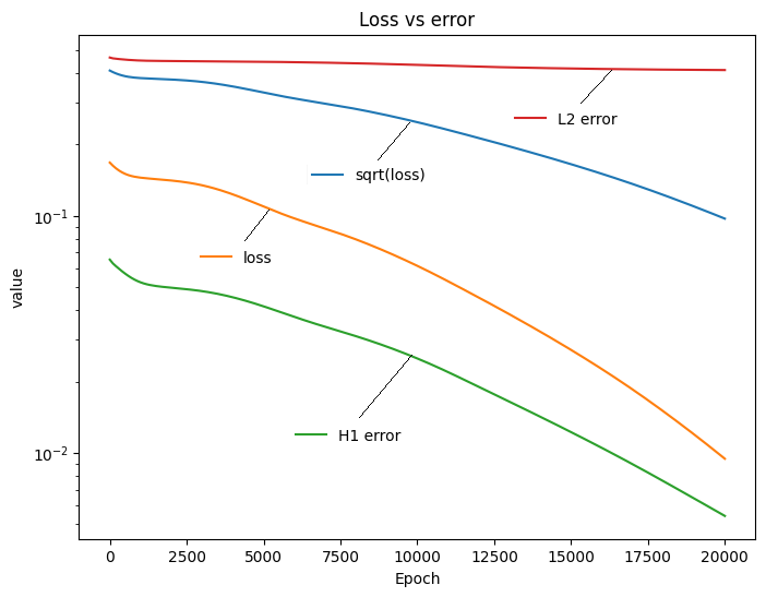
Figure 1: Convergence of PINN and the true error $H^{1}_{0}(\Omega_{h})$ for the Laplace problem with sin-sin right-hand side.

Figure 2: Solution obtained from PINN for the Laplace problem with sin-sin right-hand side.

Figure 3: The error of the solution obtained from PINN for the Laplace problem with sin-sin right-hand side.

The convergence of training with ADAM optimizer [26] is presented in Figure 1. We can see that neither loss or the square root of loss they are no equal to either the $L^{2}$ norm or $H^{1}_{0}$ norms (the true error) computed between the approximated solution $u_{\theta}$ and the exact solution (3). This loss is not robust. Changing the number of neurons or layers, or the training rate, does not help to make this lost robust.

2.2 Two-dimensional Laplace problem with exp-sin right-hand side

Given $\Omega=(0,1)^{2}\subset\mathbb{R}^{2}$ we seek the solution of the model problem with a manufactured solution

$$-\Delta u=f,$$ (6)

with zero Dirichlet b.c. In this problem, we select the solution

$$u(x_{1},x_{2})=-e^{\pi(x_{1}-2x_{2})}\sin(2\pi x_{1})\sin(\pi x_{2}).$$ (7)

In order to obtain this solution, we compute

$$f(x_{1},x_{2})=-\Delta u(x_{1},x_{2})=$$

$$=\pi^{2}e^{\pi(x-2y)}\sin(\pi y)(4\cos(2\pi x)-3\sin(2\pi x))$$ (8)

$$-\pi^{2}e^{\pi(x-2y)}\sin(2\pi x)(4\cos(\pi y)-3\sin(\pi y))$$

We define the following loss function for PINN

$$LOSS(\theta)=RES_{2}(\theta)=\sum_{\bf x}\left(\Delta u({\bf x})+f({\bf x})\right)^{2}$$ (9)

We enforce the zero Dirichlet b.c. on the NN in a strong way, following the ideas presented in [42].

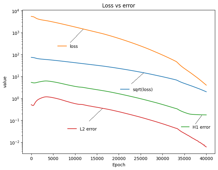
Figure 4: Convergence of PINN and the true error $H^{1}_{0}(\Omega_{h})$ for the Laplace problem with sin-exp right-hand side.

Figure 5: Solution obtained from PINN for the Laplace problem with sin-exp right-hand side.

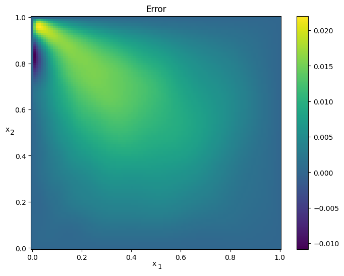
Figure 6: The error of the solution obtained from PINN for the Laplace problem with sin-exp right-hand side.

The convergence of training with ADAM optimizer [26] is presented in Figure 4. We can see that neither loss or the square root of loss they are no equal to either the $L^{2}$ norm or $H^{1}_{0}$ norms (the true error) computed between the approximated solution $u_{\theta}$ and the exact solution (7). This loss is not robust.

2.3 Two-dimensional advection-diffusion problem

Given $\Omega=(0,1)^{2}\subset\mathbb{R}^{2}$ we seek the solution $\Omega\ni(x_{1},x_{2})\rightarrow u(x_{1},x_{2})\in{\cal R}$ of the Eriksson-Johnson model problem [9], a challenging model problem designed for verification of the numerical methods.

$$\left\{\begin{array}[]{rl}\beta\cdot\nabla u-\epsilon\Delta u=0&\hbox{in }\Omega\\ u=g&\hbox{over }\partial\Omega\,,\end{array}\right.$$ (10)

with $\beta=(1,0)$, $\epsilon=0.1$, with $g$ such that

$$g(0,x_{2})=\sin\left(\pi x_{2}\right)\textrm{ for }x_{2}\in(0,1)$$ (11)

$$g(1,x_{2})=0\textrm{ for }x_{2}\in(0,1)$$ (12)

$$g(x_{1},0)=0\textrm{ for }x_{1}\in(0,1)$$ (13)

$$g(x_{1},1)=0\textrm{ for }x_{1}\in(0,1)$$ (14)

We define the shift $u_{shift}$ such that

$$u(x_{1},x_{2})=u_{0}(x_{1},x_{2})+u_{shift}(x_{1},x_{2}),$$ (15)

$$u_{shift}(x_{1},x_{2})=(1-x_{1})\sin(\pi x_{2})$$ (16)

We notice that $u_{0}(x_{1},x_{2})=u(x_{1},x_{2})-u_{shift}(x_{1},x_{2})=0$ for $(x_{1},x_{2})\in\partial\Omega$. Using the shift technique, we can transform our problem to homogenous zero Dirichlet b.c. problem: we seek $\Omega\ni(x_{1},x_{2})\rightarrow u_{0}(x_{1},x_{2})\in{\cal R}$, such that

$$\left\{\begin{array}[]{rl}\beta\cdot\nabla u_{0}-\epsilon\Delta u_{0}=-\beta\cdot\nabla u_{shift}+\epsilon\Delta u_{shift}&\hbox{in }\Omega\\ u=0&\hbox{over }\partial\Omega\,,\end{array}\right.$$ (17)

We define the following loss function for PINN

$$\begin{aligned} &LOSS(\theta)=RES_{3}(\theta)=\\ &\sum_{\bf x}\left(\beta\cdot\nabla u_{0}({\bf x})-\epsilon\Delta u_{0}({\bf x})+\beta\cdot\nabla u_{shift}({\bf x})-\epsilon\Delta u_{shift}({\bf x})\right)^{2}\end{aligned}$$ (18)

We enforce the zero Dirichlet b.c. on the NN in a strong way, following the ideas presented in [42]. To estimate the true error, we use the exact solution formula from [5]

$$u_{exact}(x,y)=\frac{(e^{(r_{1}(x-1))}-e^{(r_{2}(x-1))})}{(e^{(-r_{1})}-e^{(-r_{2})})}\sin(\pi y),$$ (19)

$$r_{1}=\frac{(1+\sqrt{(1+4\epsilon^{2}\pi^{2})})}{(2\epsilon)},r_{2}=\frac{(1-\sqrt{(1+4\epsilon^{2}\pi^{2})})}{(2\epsilon)}.$$ (20)

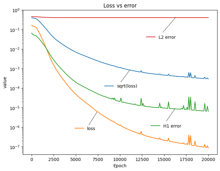
Figure 7: Convergence of PINN and the true error $\epsilon H^{1}_{0}(\Omega_{h})$ for the advection-diffusion problem.

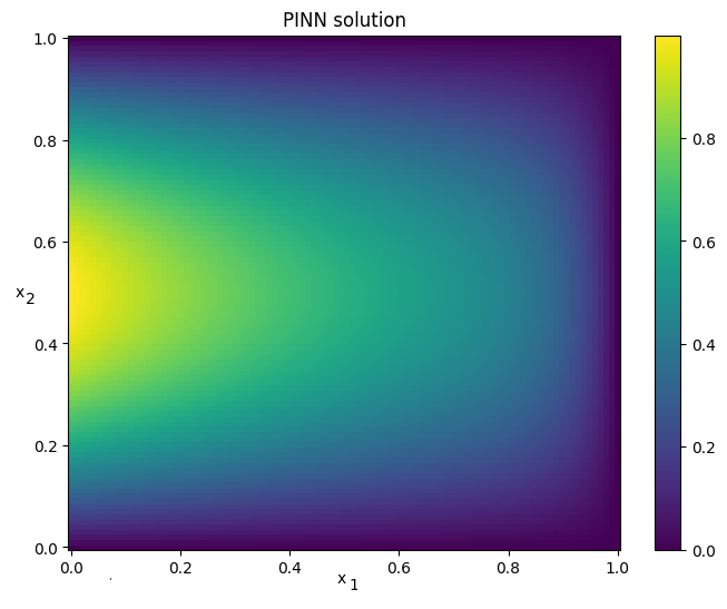
Figure 8: Solution obtained from PINN for the advection-diffusion problem.

Figure 9: The error of the solution obtained from PINN for the advection-diffusion problem.

3 Abstract framework

This section presents how to construct a robust loss function for PINN. As a reference, we refer to [39] where the mathematical theory behind the construction of the robust loss function was discussed for VPINN. In this paper, we generalize this construction for PINN.

The main conclusion from this section is summarized in Remarks 4 and 5. Remark 4 introduces the robust loss function (67) $LOSS(\theta)=RES(\theta)^{T}G^{-1}RES(\theta)$, and Remark 5 says that the true error $\|u_{\theta}-u_{EXACT}\|_{H^{1}_{0}(\Omega_{h})}$ between the approximated solution $u_{\theta}$ found by NN and the exact solution $u_{EXACT}$ is bounded by the robust loss function. We need to know how to compute the Gram matrix (66). The Gram matrix is computed using the inner product introduced in (31). Why this inner product is good? Because for this inner product and its norm (34) we can prove that the bilinear form (51) related with our PDEs is bounded (see Lemma 3 ) and inf-sup stable (see Lemma 4). Having the bounded and inf-sup stable bilinear form of our problem, we can prove Theorem 1. This theorem directly implies Remark 5 showing what we need, that the true error is bounded by our robust loss, from above and below. For other PDEs, a proper inner product must be found. This subject has been deeply studied by finite element method community [demkowicz2018dpg].

For concreteness, we shall consider the case of unit square $\Omega=(0,1)^{2}$ in 2D. Let us choose spatial resolution $N\in\mathbb{N}$ and define $h=\frac{1}{N}$. We introduce the discrete domain

$$\Omega_{h}=\{(ih,jh)\in{\mathbb{R}}^{2}:0\leq i\leq N,0\leq j\leq N\}.$$ (21)

and its interior $\Omega_{h}^{0}=\Omega_{h}\setminus\partial\Omega$, or, more explicitly

$$\Omega_{h}^{0}=\{(ih,jh)\}\in{\mathbb{R}}^{2}:0<i<N,0<j<N\}.$$ (22)

Remark 1. The points employed by the training of the PINN for evaluation of the PDE residual are selected from the $\Omega_{h}$ space, including the boundary points $\partial\Omega_{h}$.

We introduce a space of discrete functions defined over $\Omega_{h}$

$$L^{2}(\Omega_{h})=\{u\colon\Omega_{h}\rightarrow\mathbb{R}\}$$ (23)

equipped with the inner product

$$(u,v)_{L^{2}(\Omega_{h})}=h^{2}\sum_{p\in\Omega_{h}}u(p)v(p).$$ (24)

and associated norm

$$\|u\|_{L^{2}(\Omega_{h})}=(u,u)_{L^{2}(\Omega_{h})}=h^{2}\sum_{p\in\Omega_{h}}u(p)^{2}.$$ (25)

For the sake of simplicity, for $u\colon\Omega_{h}\rightarrow\mathbb{R}$ we denote

$$u_{i,j}=u(x_{i,j})=u(ih,jh).$$ (26)

Next, we introduce the discrete gradient operators

$$\nabla_{+}u_{i,j}=\left(\nabla_{x+}u_{i,j},\nabla_{y+}u_{i,j}\right)=\left(\frac{u_{i+1,j}-u_{i,j}}{h},\frac{u_{i,j+1}-u_{i,j}}{h}\right).$$ (27)

$$\nabla_{-}u_{i,j}=\left(\nabla_{x-}u_{i,j},\nabla_{y-}u_{i,j}\right)=\left(\frac{u_{i,j}-u_{i-1,j}}{h},\frac{u_{i,j}-u_{i,j-1}}{h}\right).$$ (28)

These gradients can be treated as discrete functions on $\Omega_{h}$, if we define their value to be $0$ for points where the above definition is not valid. Standard 5-point discrete Laplace operator

$$\Delta_{h}u_{i,j}=\frac{1}{h^{2}}\left(u_{i+1,j}+u_{i-1,j}+u_{i,j+1}+u_{i,j-1}-4u_{i,j}\right).$$ (29)

can be expressed as $\Delta_{h}=\nabla_{+}\circ\nabla_{-}=\nabla_{-}\circ\nabla_{+}$. We can use the discrete gradients to define another space

$$H^{1}_{0}(\Omega_{h})=\{u\in{L^{2}(\Omega_{h})}:\left.u\right|_{\partial\Omega}=0\}.$$ (30)

with an inner product and the induced norm

$$(u,v)_{H^{1}_{0}(\Omega_{h})}=(\nabla_{x+}u,\nabla_{x+}v)_{L^{2}(\Omega_{h})}+(\nabla_{y+}u,\nabla_{y+}v)_{L^{2}(\Omega_{h})}$$ (31)

$$=\sum_{\begin{subarray}{c}0\leq i<N\\ 0\leq j\leq N\end{subarray}}(u_{i+1,j}-u_{i,j})(v_{i+1,j}-v_{i,j})+$$ (32)

$$\sum_{\begin{subarray}{c}0\leq i\leq N\\ 0\leq j<N\end{subarray}}(u_{i,j+1}-u_{i,j})(v_{i,j+1}-v_{i,j}).$$ (33)

$$\|u\|_{H^{1}_{0}(\Omega_{h})}=(u,u)_{H^{1}_{0}(\Omega_{h})}.$$ (34)

We introduce discrete test functions $\Omega_{h}\ni x\mapsto\delta_{i,j}(x)\in{\mathbb{R}}$

$$\delta_{i,j}(x)=\displaystyle{\left\{\begin{aligned} &1\quad\textrm{ for }x=x_{i,j}\\ &0\quad\textrm{ otherwise }\end{aligned}\right.}.$$ (35)

Then $\mathcal{B}=\{\delta_{i,j}\}_{0<i,j<N}$ constitutes a basis of $H^{1}_{0}(\Omega_{h})$.

Remark 2. In PINN method the discrete test functions represent the discrete Dirac deltas of the training points.

Lemma 1 (Discrete integration by parts).

Given $u\in{H^{1}_{0}(\Omega_{h})}$, $v\in{L^{2}(\Omega_{h})}$ we have

$$\left(\nabla_{x+}u,v\right)_{L^{2}(\Omega_{h})} =-\left(u,\nabla_{x+}v\right)_{L^{2}(\Omega_{h})}$$ (36)

$$\left(\nabla_{y+}u,v\right)_{L^{2}(\Omega_{h})} =-\left(u,\nabla_{y+}v\right)_{L^{2}(\Omega_{h})}$$

Proof.

Since the scalar product is bilinear, it is enough to demonstrate the above for basis functions $u=\delta_{i,j}$. We have

$$\nabla_{x+}\delta_{i,j}=\begin{cases}\phantom{-}h^{-1}&\text{at }x_{i-1,j}\\ -h^{-1}&\text{at }x_{i,j}\\ 0&\text{elsewhere}\end{cases}$$ (37)

$$\left(\nabla_{x+}\delta_{i,j},v\right)_{L^{2}(\Omega_{h})} =h^{-1}u_{i-1,j}+\left(-h^{-1}\right)u_{i,j}$$ (38)

$$=-\nabla_{x+}u_{i,j}=-\left(\delta_{i,j},\nabla_{x+}v\right)_{L^{2}(\Omega_{h})}$$

For $\nabla_{y+}$ the proof is similar. ∎

Discrete gradients also satisfy an analogue of the product rule. For any $f,g\colon\Omega_{h}\rightarrow\mathbb{R}$ we have

$$\nabla_{x+}(fg)_{i,j} =f_{i+1,j}g_{i+1,j}-f_{i,j}g_{i,j}$$ (39)

$$=f_{i+1,j}g_{i+1,j}-f_{i+1,j}g_{i,j}+f_{i+1,j}g_{i,j}-f_{i,j}g_{i,j}$$

$$=f_{i+1,j}(\nabla_{x+}g)_{i,j}+(\nabla_{x+}f)_{i,j}g_{i,j}$$

Let us define a translation operator $\tau_{x}\colon{L^{2}(\Omega_{h})}\rightarrow{L^{2}(\Omega_{h})}$ as

$$(\tau_{x}u)_{i,j}=\begin{cases}u_{i+1,j}&\text{for }i<N\\ 0&\text{otherwise}\end{cases}$$ (40)

Then we can write $\nabla_{x+}(fg)=\tau_{x}f(\nabla_{x+}g)+(\nabla_{x+}f)g$. Furthermore, for $f\in{H^{1}_{0}(\Omega_{h})}$, $\|\tau_{x}f\|_{L^{2}(\Omega_{h})}=\|f\|_{L^{2}(\Omega_{h})}$, since only the zero boundary values get shifted out of the domain.

Lemma 2 (Discrete Poincaré).

There exists a constant $C>0$ independent of $N$, such that for all $u\in{H^{1}_{0}(\Omega_{h})}$ we have

$$\|u\|_{L^{2}(\Omega_{h})}\leq C\|u\|_{H^{1}_{0}(\Omega_{h})}$$ (41)

Proof.

Let us define $\phi\in{L^{2}(\Omega_{h})}$ by $\phi_{i,j}=ih$. Then $\nabla_{x+}\phi=1$ in $\Omega_{h}^{0}$, and

$$\|u\|_{L^{2}(\Omega_{h})}^{2}=(u,u)_{L^{2}(\Omega_{h})}=\left(1,u^{2}\right)_{L^{2}(\Omega_{h})}\left(\nabla_{x+}\phi,u^{2}\right)_{L^{2}(\Omega_{h})}=$$ (42)

$$-\left(\phi,\nabla_{x+}u^{2}\right)_{L^{2}(\Omega_{h})}=-\left(\phi,(u+\tau_{x}u)\nabla_{x+}u\right)_{L^{2}(\Omega_{h})}$$

Applying the Cauchy-Schwartz inequality, we get

$$\|u\|_{L^{2}(\Omega_{h})}^{2} \leq\|\phi\|_{L^{2}(\Omega_{h})}\left[\|u\|_{L^{2}(\Omega_{h})}+\|\tau_{x}u\|_{L^{2}(\Omega_{h})}\right]\|\nabla_{x+}u\|_{L^{2}(\Omega_{h})}$$ (43)

$$=2\|\phi\|_{L^{2}(\Omega_{h})}\|u\|_{L^{2}(\Omega_{h})}\|\nabla_{x+}u\|_{L^{2}(\Omega_{h})}$$

$$\|u\|_{L^{2}(\Omega_{h})}\leq 2\|\phi\|_{L^{2}(\Omega_{h})}\|\nabla_{x+}u\|_{L^{2}(\Omega_{h})}$$ (44)

Furthermore, since $|\phi_{i,j}|\leq 1$, we have

$$\|\phi\|_{L^{2}(\Omega_{h})}\leq\|1\|_{L^{2}(\Omega_{h})}=1$$ (45)

$$\|u\|_{L^{2}(\Omega_{h})}\leq 2\|\phi\|_{L^{2}(\Omega_{h})}\|\nabla_{x+}u\|_{L^{2}(\Omega_{h})}\leq 2\|u\|_{H^{1}_{0}(\Omega_{h})}$$ (46)

independently of the mesh size $N$.

∎

Let us focus on the advection-diffusion problem:

$$\textrm{We seek }u\in H^{1}_{0}(\Omega_{h}):\beta_{x}\nabla_{x+}u+\beta_{x}\nabla_{y+}u-\epsilon\Delta_{h}u=f,$$ (47)

where $f\in L^{2}(\Omega_{h})$ is a given function. We compute the inner product with test functions functions $v\in H^{1}_{0}(\Omega_{h})$

$$(\beta_{x}\nabla_{x+}u,v)_{L^{2}(\Omega_{h})}+(\beta_{y}\nabla_{y+}u,v)_{L^{2}(\Omega_{h})}$$ (48)

$$-\epsilon(\Delta_{h}u,v)_{L^{2}(\Omega_{h})}=(f,v)_{L^{2}(\Omega_{h})}\ \forall v\in H^{1}_{0}(\Omega_{h}).$$

Applying Lemma 1 to the term with the Laplacian, we get

$$-(\Delta_{h}u,v)_{L^{2}(\Omega_{h})}=(\nabla_{+}u,\nabla_{+}v)_{L^{2}(\Omega_{h})},$$ (49)

We apply it for the left-hand side of (48)

$$(\beta_{x}\nabla_{x+}u,v)_{L^{2}(\Omega_{h})}+(\beta_{y}\nabla_{y+}u,v)_{L^{2}(\Omega_{h})}+$$ (50)

$$\epsilon(\nabla_{+}u,\nabla_{+}v)_{L^{2}(\Omega_{h})}=(f,v)_{L^{2}(\Omega_{h})}.$$

Our advection-diffusion problem has been reformulated in the discrete weak form as: Find $u\in H^{1}_{0}(\Omega_{h})$ such that

$$b(u,v)=l(v)\quad\forall v\in{H^{1}_{0}(\Omega_{h})}$$ (51)

$$b(u,v)=(\beta_{x}\nabla_{x+}u,v)_{L^{2}(\Omega_{h})}+$$ (52)

$$(\beta_{y}\nabla_{y+}u,v)_{L^{2}(\Omega_{h})}+\epsilon(\nabla_{+}u,\nabla_{+}v)_{L^{2}(\Omega_{h})},$$

$$l(v)=(f,v)_{L^{2}(\Omega_{h})}.$$ (53)

The residual of the advection-diffusion problem is

$$r(u,v)=b(u,v)-l(v).$$ (54)

We can form a vector of residuals $\{r(u,\delta_{i,j})\}_{0<i,j<N}$.

Lemma 3.

The form $b(u,v)$ of the discrete weak formulation (51) is a bounded bilinear form in the norm (31). This means that there exists $\mu$ independent of $N$ such that

$$b(u,v)\leq\mu\|u\|_{H^{1}_{0}(\Omega_{h})}\|v\|_{H^{1}_{0}(\Omega_{h})},\forall u,v\in{H^{1}_{0}(\Omega_{h})}$$ (55)

Proof.

We have

$$b(u,v) =\epsilon(u,v)_{H^{1}_{0}(\Omega_{h})}+(\beta_{x}\nabla_{x+}u,v)+(\beta_{y}\nabla_{y+}u,v)$$ (56)

$$\leq\epsilon\|u\|_{H^{1}_{0}(\Omega_{h})}\|v\|_{H^{1}_{0}(\Omega_{h})}+2\|\beta\|_{\infty}\|u\|_{H^{1}_{0}(\Omega_{h})}\|v\|_{L^{2}(\Omega_{h})}$$

where $\|\beta\|_{\infty}=\max\{|\beta_{x}|,|\beta_{y}|\}$. By Lemma 2, we have $C>0$ such that $\|v\|_{L^{2}(\Omega_{h})}\leq C\|v\|_{H^{1}_{0}(\Omega_{h})}$, so

$$b(u,v)\leq(\epsilon+2C\|\beta\|_{\infty})\|u\|_{H^{1}_{0}(\Omega_{h})}\|v\|_{H^{1}_{0}(\Omega_{h})}$$ (57)

which proves the boundedness of $b$. ∎

Lemma 4.

The form $b(u,v)$ of the discrete weak formulation (51) is inf-sup stable bilinear form in the norm (31), if $2\epsilon>MC^{2}$, where $C>0$ is the constant from Lemma 2, and $M=\max_{i,j}\left|\nabla_{x+}\beta_{x}+\nabla_{y+}\beta_{y}\right|$. This means that there exists $\alpha>0$ independent of $N$ such that

$$\sup_{0\neq v\in V}\frac{b(u,v)}{\|v\|_{H^{1}_{0}(\Omega_{h})}}\geq\alpha\|u\|_{H^{1}_{0}(\Omega_{h})},\forall u\in{H^{1}_{0}(\Omega_{h})}$$ (58)

In particular, the condition is fulfilled for constant $\beta_{x},\beta_{y}$.

Proof.

We have

$$(\beta_{x}\nabla_{x+}u,u)_{L^{2}(\Omega_{h})} =(\nabla_{x+}u,\beta_{x}u)_{L^{2}(\Omega_{h})}=-(u,\nabla_{x+}(\beta_{x}u))_{L^{2}(\Omega_{h})}$$

$$=-(u,\beta_{x}\nabla_{x+}u)_{L^{2}(\Omega_{h})}-(u,\tau_{x}u\,(\nabla_{x+}\beta_{x})_{L^{2}(\Omega_{h})}$$

$$(\beta_{x}\nabla_{x+}u,u)_{L^{2}(\Omega_{h})}=-\frac{1}{2}\left(u,\tau_{x}u\,(\nabla_{x+}\beta_{x})\right)_{L^{2}(\Omega_{h})}$$

Similar identity holds for $\nabla_{y+}$. Adding these together we get

$$\left|(\beta_{x}\nabla_{x+}u,u)_{L^{2}(\Omega_{h})}+(\beta_{y}\nabla_{y+}u,u)_{L^{2}(\Omega_{h})}\right|$$ (59)

$$\leq\frac{1}{2}\left|\left(u,\tau_{x}u\,(\nabla_{x+}\beta_{x}+\nabla_{y+}\beta_{y})\right)_{L^{2}(\Omega_{h})}\right|$$

$$\leq\frac{1}{2}\|\nabla_{x+}\beta_{x}+\nabla_{y+}\beta_{y}\|_{\infty}\|u\|^{2}_{L^{2}(\Omega_{h})}$$

$$=\frac{1}{2}M\|u\|^{2}_{L^{2}(\Omega_{h})}\leq\frac{1}{2}MC^{2}\|u\|^{2}_{H^{1}_{0}(\Omega_{h})}$$

$$b(u,u) =\epsilon(\nabla_{x+}u,\nabla_{x+}u)_{L^{2}(\Omega_{h})}+(\beta_{x}\nabla_{x+}u+\beta_{y}\nabla_{y+}u,u)_{L^{2}(\Omega_{h})}$$

$$\geq\epsilon\|u\|^{2}_{H^{1}_{0}(\Omega_{h})}-\left|(\beta_{x}\nabla_{x+}u+\beta_{y}\nabla_{y+}u,u)_{L^{2}(\Omega_{h})}\right|$$

$$\geq\underbrace{\left(\epsilon-\frac{1}{2}MC^{2}\right)}_{>0}\|u\|^{2}_{H^{1}_{0}(\Omega_{h})}$$

∎

Given a $u\in{H^{1}_{0}(\Omega_{h})}$, we can find $\phi\in{H^{1}_{0}(\Omega_{h})}$ such that

$$(\phi,v)_{H^{1}_{0}(\Omega_{h})}=r(u,v)\quad\forall v\in{H^{1}_{0}(\Omega_{h})}$$ (60)

We will call such $\phi$ the residual representative. The following theorem establishes a relation between the norm of $\phi$ and the difference between $u$ and $u_{\text{EXACT}}$, where $u_{\text{EXACT}}$ denotes the solution of the weak problem (51).

Theorem 1.

Let $u\in{H^{1}_{0}(\Omega_{h})}$ and $\phi$ be its residual representative. Then

$$\frac{1}{\mu}\|\phi\|_{H^{1}_{0}(\Omega_{h})}\leq\|u-u_{\text{EXACT}}\|_{H^{1}_{0}(\Omega_{h})}\leq\frac{1}{\alpha}\|\phi\|_{H^{1}_{0}(\Omega_{h})}$$ (61)

where $\mu$, $\alpha$ are the boundedness and inf-sup constants of $b$.

Proof.

The general idea of this proof is based on the similar considerations for the continuous case of Robust Variational Physics Informed Neural Networks introduced in [39]. By definition of $\phi$, we have

$$\|\phi\|_{H^{1}_{0}(\Omega_{h})}=\sup_{0\neq w\in{H^{1}_{0}(\Omega_{h})}}\frac{(\phi,w)_{H^{1}_{0}(\Omega_{h})}}{\|w\|_{H^{1}_{0}(\Omega_{h})}}=\sup_{0\neq w\in{H^{1}_{0}(\Omega_{h})}}\frac{r(u,w)}{\|w\|_{H^{1}_{0}(\Omega_{h})}}$$

$$=\sup_{0\neq w\in{H^{1}_{0}(\Omega_{h})}}\frac{b(u,w)-l(w)}{\|w\|_{H^{1}_{0}(\Omega_{h})}}=\sup_{0\neq w\in{H^{1}_{0}(\Omega_{h})}}\frac{b(u-u_{\text{EXACT}},w)}{\|w\|_{H^{1}_{0}(\Omega_{h})}}$$

From the inf-sup condition we get

$$\sup_{0\neq w\in{H^{1}_{0}(\Omega_{h})}}\frac{(\phi,w)_{H^{1}_{0}(\Omega_{h})}}{\|w\|_{H^{1}_{0}(\Omega_{h})}}\geq\alpha\|u-u_{\text{EXACT}}\|_{H^{1}_{0}(\Omega_{h})}$$ (62)

which proves the right inequality. The left one follows from boundedness of $b$:

$$\sup_{0\neq w\in{H^{1}_{0}(\Omega_{h})}}\frac{(\phi,w)_{H^{1}_{0}(\Omega_{h})}}{\|w\|_{H^{1}_{0}(\Omega_{h})}}\leq\mu\|u-u_{\text{EXACT}}\|_{H^{1}_{0}(\Omega_{h})}.$$ (63)

∎

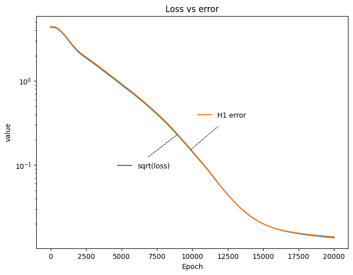
Figure 10: Convergence of RPINN and the true error $H^{1}_{0}(\Omega_{h})$.

We can use this theorem to construct a robust loss function

$$\text{LOSS}(\theta)=\|\phi\|_{H^{1}_{0}(\Omega_{h})}^{2}$$ (64)

Given $u\in{H^{1}_{0}(\Omega_{h})}$, we can construct the vector of residuals $\text{RES}=\{r(u,\phi_{i,j})\}_{0<i,j<N}$. Coefficients $\Phi\in\mathbb{R}^{N\times N}$ of the residual representative $\phi$ fullfill $\text{RES}=G\Phi$ where $G$ is the Gram matrix of scalar product of ${H^{1}_{0}(\Omega_{h})}$. So,

$$\|\phi\|_{H^{1}_{0}(\Omega_{h})}^{2} =\Phi^{T}G\Phi=(G^{-1}\text{RES})^{T}G\,G^{-1}\text{RES}$$ (65)

$$=\text{RES}^{T}G^{-1}\text{RES}$$

We will construct now the Gram matrix $G_{i,j;k,l}=(\delta_{i,j},\delta_{k,l})_{H^{1}_{0}(\Omega_{h})}$, using the norm of $H^{1}_{0}(\Omega_{h})$ space

$$G_{i,j;k,l}= h^{-2}\displaystyle{\left\{\begin{aligned} &\phantom{-}\,\,4\ \quad\textrm{ for }(i,j)=(k,l)\\ &-1\quad\textrm{ for }(k,l)\in\{(i+1,j),(i-1,j)\}\\ &-1\quad\textrm{ for }(k,l)\in\{(i,j+1),(i,j-1)\}\end{aligned}\right.}$$ (66)

Remark 3. The inner product selected for the Gram matrix is induced by the norm for which the form $b(u,v)$ of the discrete weak formulation (51) is a bounded inf-sup stable.

Remark 4. The Gram matrix of the inner product of $H^{1}_{0}(\Omega_{h})$ is sparse, and it can be efficiently inverted.

The following robust loss function implies.

$$LOSS(\theta)=RES(\theta)^{T}{\bf G}^{-1}RES(\theta)$$ (67)

Remark 5. For a neural network solution $u_{\theta}$, the norm for which the form $b(u,v)$ of the discrete weak formulation (51) is a bounded inf-sup stable, for $u_{\text{EXACT}}$ the exact solution of (51), and for the robust loss function $LOSS(\theta)$ it holds

$$\frac{\sqrt{LOSS(\theta)}}{\mu}\leq\|u_{\theta}-u_{EXACT}\|_{H^{1}_{0}(\Omega_{h})}\leq\frac{\sqrt{LOSS({\theta})}}{\alpha}$$ (68)

For the Laplace problems, $\mu=\alpha=1$.

4 Numerical results for the Robust Physics Informed Neural Networks

In this section, we solve the same three two-dimensional model problems as in Section 2, but this time by using RPINN, namely, the modified loss function. The goal of this section is to illustrate that in our RPINN method, the loss function is very close to the true

4.1 Two-dimensional Laplace problem with sin-sin right-hand side

We solve the identical problem as in Section 2.1, namely we seek the solution of $-\Delta u=f$ with zero Dirichlet b.c. with $f(x_{1},x_{2})=8\pi^{2}\sin(2\pi x_{1})\sin(2\pi x_{2})$. This time we define the following loss function for RPINN

$$LOSS(\theta)=RES_{1}^{T}(\theta)\times{\bf G}^{-1}\times RES_{1}(\theta)$$ (69)

with $RES_{1}(\theta)$ defined by (5) and Gram matrix defined by (66).

Figure 11: Convergence of RPINN and the true error $H^{1}_{0}(\Omega_{h})$ for the Laplace problem with sin-sin right-hand side.

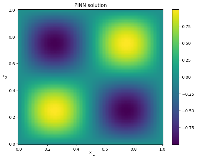
Figure 12: Solution obtained from RPINN for the Laplace problem with sin-sin right-hand side.

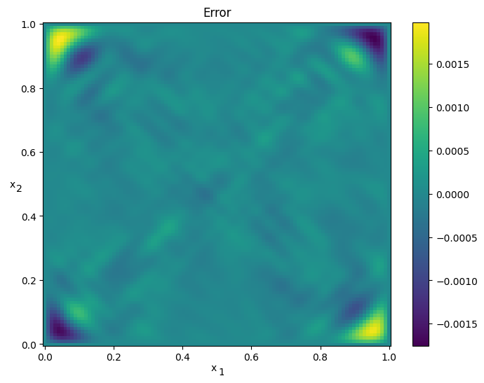
Figure 13: The error of the solution obtained from RPINN for the Laplace problem with sin-sin right-hand side.

The convergence of training with ADAM optimizer [26] is presented in Figure 11. We can see that our loss is robust and equal to the true error computed in (31) norm. This is because for the Laplace problem we have $\mu=\alpha=1$ so $\sqrt{LOSS(\theta)}=\|u_{EXACT}-u_{\theta}\|_{H^{1}_{0}(\Omega_{h})}$. The obtained solution is presented in Figure 12.

4.2 Two-dimensional Laplace problem with exp-sin right-hand side

Here we solve identical problem as in Section 2.2, namely $-\Delta u=f$ with zero Dirichlet b.c., with $f(x_{1},x_{2})=\pi^{2}e^{\pi(x-2y)}\sin(\pi y)(4\cos(2\pi x)-3\sin(2\pi x))-\pi^{2}e^{\pi(x-2y)}\sin(2\pi x)(4\cos(\pi y)-3\sin(\pi y))$. This time we define the following loss function for RPINN

$$LOSS(\theta)=RES_{2}^{T}(\theta)\times{\bf G}^{-1}\times RES_{2}(\theta)$$ (70)

with $RES_{2}(\theta)$ defined by (9) and Gram matrix defined by (66).

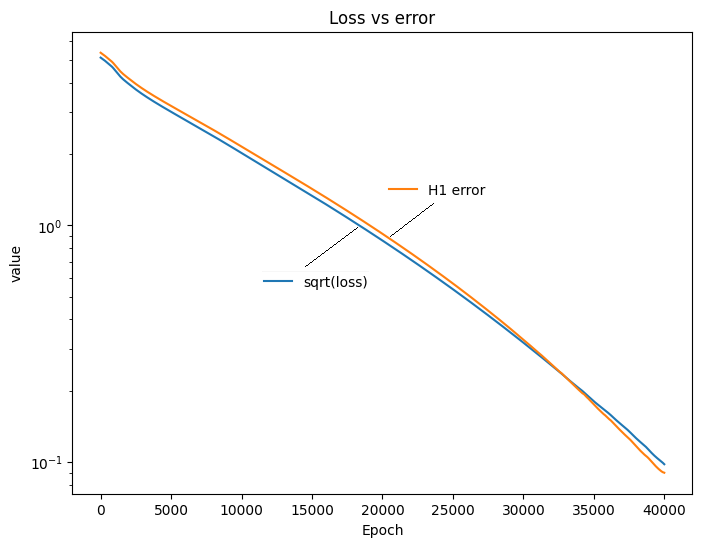
Figure 14: Convergence of RPINN and the true error $H^{1}_{0}(\Omega_{h})$ for the Laplace problem with sin-exp right-hand side.

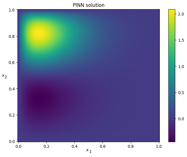
Figure 15: Solution obtained from RPINN for the Laplace problem with sin-exp right-hand side.

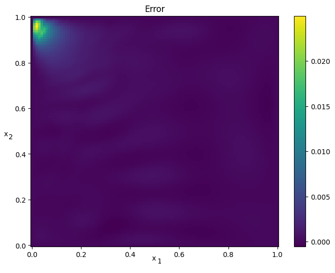
Figure 16: The error of the solution obtained from RPINN for the Laplace problem with sin-exp right-hand side.

The convergence of training with ADAM optimizer [26] is presented in Figure 14. We can see that our loss is robust and equal to the true error computed in (31) norm. Again, for the Laplace problem $\mu=\alpha=1$ and $\sqrt{LOSS(\theta)}=\|u_{EXACT}-u_{\theta}\|_{H^{1}_{0}(\Omega_{h})}$. The obtained solution is presented in Figure 15.

4.3 Two-dimensional advection-diffusion problem

Finally, we solve the Eriksson-Johnson model problem described in Section 2.3 introduced in [9], analysed in [4]. Namely, we solve $\beta\cdot\nabla u-\epsilon\Delta u=0$ with zero Dirichlet b.c. except the left side of the domain, where $u(0,x_{2})=\sin\left(\pi x_{2}\right)$ for $x_{2}\in(0,1)$. This time we define the following loss function for RPINN

$$LOSS(\theta)=RES_{3}(\theta)^{T}\times{\bf G}^{-1}\times RES_{3}(\theta)$$ (71)

with $RES_{3}(\theta)$ defined by (18) and Gram matrix defined by (66).

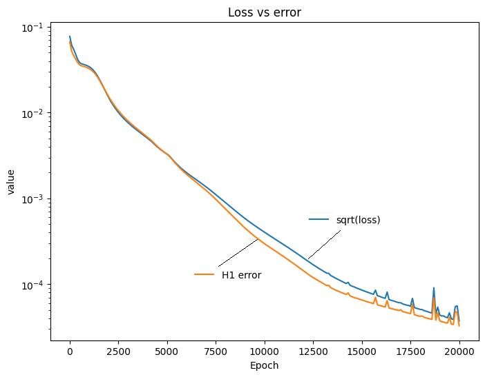
Figure 17: Convergence of PINN and the true error $\epsilon H^{1}_{0}(\Omega_{h})$.

Figure 18: Solution obtained from RPINN for the advection-diffusion problem.

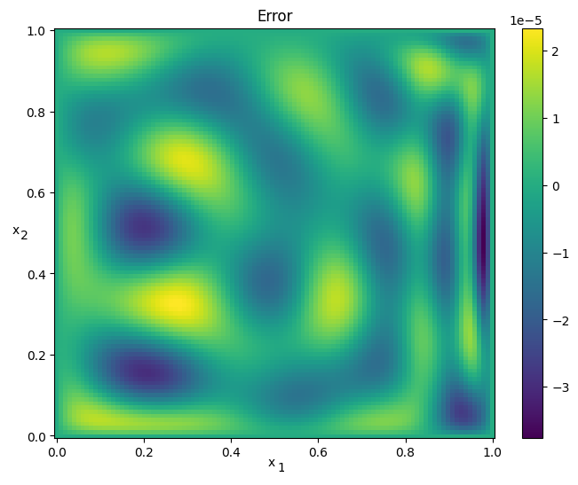
Figure 19: The error of the solution obtained from RPINN for the advection-diffusion problem.

The convergence of training with ADAM optimizer [26] is presented in Figure 17. For the advection-diffsion, $\mu=(\epsilon+2C)=(0.1+2\times 2)=4.1$, and $\alpha=\epsilon=0.1$. So we have $\frac{1}{4.1}\sqrt{LOSS(\theta)}\leq\|u_{EXACT}-u_{\theta}\|_{H^{1}_{0}(\Omega_{h})}\leq\frac{1}{0.1}\sqrt{LOSS(\theta)}$. Multiplying by $\epsilon=0.1$, we have $\frac{1}{41}\sqrt{LOSS(\theta)}\leq 0.1\times\|u_{EXACT}-u_{\theta}\|_{H^{1}_{0}(\Omega_{h})}\leq\sqrt{LOSS(\theta)}$. This implies the agreement of the plots if we measure the error in $\epsilon H^{1}_{0}(\Omega_{h})$ norm. The robust loss function and the true error are close to each other. The obtain solution is presented in Figure 18.

5 Computational code

The python code for the experiments performed in this paper is avaialble for running in Google Colab.

https://colab.research.google.com/drive/1ZGPFkAl6OQazSFAPXYC_E-MvXgR_JN2f

The parameters are the following:

• LENGTH_X = 1., TOTAL_TIME = 1. denotes the spatial dimensions of the computational domain, $(0,LENGTH\_X)\times(0,TOTAL\_TIME)$. The variables in the code are denoted by $(x,t)$,

• N_POINTS_X = 100 number of uniformly distributed points along $x$ direction, namely $N_{x}+1$,

• N_POINTS_T = 100 number of uniformly distributed points along $t$ direction, namely $N_{y}+1$,

• LAYERS = 2 number of layers of neural network,

• NEURONS_PER_LAYER = 100 number of neurons per layer,

• EPOCHS = 20_000 number of epochs for training (for first and third problem set to 20_000, for the second problem set to 40_000),

• LEARNING_RATE = 0.0001 learning rate coefficient for training,

• RPINN = 0 turns off RPINN=0 or turns on RPINN=1 the robust loss function,

• EXAMPLE = 1 selects the examples according to Section 2.

The execution of RVPINN examples with this setup of parameters on V100 GPGPU from Google ColabPro takes less than 5 minutes, as for January 4, 2024. This includes connecting and setting up the virtual environment, and generating output pictures. Thus, we can solve these problems within 4 minute using RVPINN method.

6 Conclusions

In this article, we proposed an alternative way of constructing the loss functionals for PINNs. We numerically show the robustness of our loss function. For all the numerical examples, it can be used as the true error estimator. Our robust loss function involves the inverse of the Gram matrix computed for the special inner product. The norm related to this inner product allows us to show that the bilinear form of the weak formulation of our PDE is bounded and unstable. This project is the transfer of knowledge from the theory of finite element methods into the PINN world.

Summing up, the robust loss function for PINN is given by the norm of the vector of residuals computed at various points, induced by the inverse of the Gram matrix. Namely,

• We select the PDE, e.g., the advection-diffusion, and we derive its discrete weak formulation, e.g. (51)

• We seek the inner product for which the form $b(u_{i,j},v_{i,j})$ of the discrete weak formulation (51) is a bounded inf-sup stable bilinear form in the induced norm. For the advection-diffusion, we select the inner product (31).

• We select the test functions. In the case of PINN, they correspond with the points selected for training, and they are given by (35), namely $\{\delta_{i,j}(x)\}_{i,j}$.

• We compute the Gram matrix ${\bf G}$, the inner products of the test functions. In our case, with test functions given by (35), and the inner product given by (31), the Gram matrix is prescribed by (66).

• We invert the sparse Gram matrix.

• The robust loss function is defined as $LOSS(\theta)=RES(\theta)^{T}{\bf G}^{-1}RES(\theta)$

The future work may involve extension of the method to other classical problems solved by finite element method [Ern], including fluid flow problems [16], structural analysis [8], phase-field problems [14], or space-time problems [11].

7 Acknowledgments

This work was supported by the program ,,Excellence initiative - research university” for the AGH University of Krakow. The Authors are thankful for support from the funds assigned to AGH University of Krakow by the Polish Ministry of Science and Higher Education.

References

• Alber et al. [2019] Mark Alber, Adrian Buganza Tepole, William R. Cannon, Suvranu De, Salvador Dura-Bernal, Krishna Garikipati, George Karniadakis, William W. Lytton, Paris Perdikaris, Linda Petzold, and Ellen Kuhl. Integrating machine learning and multiscale modeling-perspectives, challenges, and opportunities in the biologica biomedical, and behavioral sciences. NPJ Digital Medicine, 2, 2019.
• Badia et al. [2024] Santiago Badia, Wei Li, and Alberto F. Martin. Finite element interpolated neural networks for solving forward and inverse problems. Computer Methods in Applied Mechanics and Engineering, 418(A), 2024.
• Cai et al. [2021] Shengze Cai, Zhiping Mao, Zhicheng Wang, Minglang Yin, and George Em Karniadakis. Physics-informed neural networks (PINNs) for fluid mechanics: A review. Acta Mechanica Sinica, 37(12):1727–1738, 2021.
• Calo et al. [2021] V.M. Calo, M. Łoś, Q. Deng, I. Muga, and M. Paszyński. Isogeometric residual minimization method (igrm) with direction splitting preconditioner for stationary advection-dominated diffusion problems. Computer Methods in Applied Mechanics and Engineering, 373:113214, 2021.
• Chan et al. [2014] Jesse Chan, Norbert Heuer, Tan Bui-Thanh, and Leszek Demkowicz. A robust DPG method for convection-dominated diffusion problems II: Adjoint boundary conditions and mesh-dependent test norms. Computers & Mathematics with Applications, 67(4):771–795, 2014.
• Chaumont-Frelet and Ern [2023] Théophile Chaumont-Frelet and Alexandre Ern. Asymptotic optimality of the edge finite element approximation of the time-harmonic Maxwell’s equations. hal-04216433, September 2023.
• Chen et al. [2020] Yuyao Chen, Lu Lu, George Em Karniadakis, and Luca Dal Negro. Physics-informed neural networks for inverse problems in nano-optics and metamaterials. Optics express, 28(8):11618–11633, 2020.
• Cottrell et al. [2007] J.A. Cottrell, T.J.R. Hughes, and A. Reali. Studies of refinement and continuity in isogeometric structural analysis. Computer Methods in Applied Mechanics and Engineering, 196(41):4160–4183, 2007.
• Eriksson and Johnson [1991] Kenneth Eriksson and Claes Johnson. Adaptive finite element methods for parabolic problems i: A linear model problem. SIAM J. Num. Anal., 28(1):43–77, 1991.
• Fangzheng Sun [2021] Hao Sun Fangzheng Sun, Yang Liu2. Physics-informed spline learning for nonlinear dynamics discovery. Proceedings of the Thirtieth International Joint Conference on Artificial Intelligence (IJCAI-21), pages 2054–2061, 2021.
• Führer and Karkulik [2021] Thomas Führer and Michael Karkulik. Space–time least-squares finite elements for parabolic equations. Computers & Mathematics with Applications, 92:27–36, 2021.
• Geneva and Zabaras [2020] Nicholas Geneva and Nicholas Zabaras. Modeling the dynamics of pde systems with physics-constrained deep auto-regressive networks. Journal of Computational Physics, 403, 2020.
• Gheisari et al. [2017] Mehdi Gheisari, Guojun Wang, and Md Zakirul Alam Bhuiyan. A survey on deep learning in big data. In 2017 IEEE international conference on computational science and engineering (CSE) and IEEE international conference on embedded and ubiquitous computing (EUC), volume 2, pages 173–180. IEEE, 2017.
• Gomez et al. [2014] Hector Gomez, Alessandro Reali, and Giancarlo Sangalli. Accurate, efficient, and (iso)geometrically flexible collocation methods for phase-field models. Journal of Computational Physics, 262:153–171, 2014.
• Goswami et al. [2020] Somdatta Goswami, Cosmin Anitescu, Souvik Chakraborty, and Timon Rabczuk. Transfer learning enhanced physics informed neural network for phase-field modeling of fracture. Theoretical and applied fracture machanics, 106, 2020.
• Guermond and Minev [2011] J.L. Guermond and P.D. Minev. A new class of massively parallel direction splitting for the incompressible navier–stokes equations. Computer Methods in Applied Mechanics and Engineering, 200(23):2083–2093, 2011.
• Hinton et al. [2012] Geoffrey Hinton, Li Deng, Dong Yu, George E Dahl, Abdel-rahman Mohamed, Navdeep Jaitly, Andrew Senior, Vincent Vanhoucke, Patrick Nguyen, Tara N Sainath, et al. Deep neural networks for acoustic modeling in speech recognition: The shared views of four research groups. IEEE Signal processing magazine, 29(6):82–97, 2012.
• Huang et al. [2022a] Shenglin Huang, Zequn He, Bryan Chem, and Celia Reina. Variational onsager neural networks (vonns): A thermodynamics-based variational learning strategy for non-equilibrium pdes. Journal of the mechanics and physics of solids, 163, 2022.
• Huang et al. [2022b] Xiang Huang, Hongsheng Liu, Beiji Shi, Zidong Wang, Kang Yang, Yang Li, Min Wang, Haotian Chu, Jing Zhou, Fan Yu, Bei Hua, Bin Dong, and Lei Chen. A universal pinns method for solving partial differential equations with a point source. Proceedings of the Fourteen International Joint Conference on Artificial Intelligence (IJCAI-22), pages 3839–3846, 2022.
• Jagtap et al. [2020] Ameya D. Jagtap, Kenji Kawaguchi, and George Em Karniadakis. Adaptive activation functions accelerate convergence in deep and physics-informed neural networks. Journal of Computational Physics, 404, 2020.
• Jin et al. [2022] Henry Jin, Marios Mattheakis, and Pavlos Protopapas. Physics-informed neural networks for quantum eigenvalue problems. In 2022 International Joint Conference on Neural Networks (IJCNN), pages 1–8, 2022.
• Kharazmi et al. [2019] Ehsan Kharazmi, Zhongqiang Zhang, and George Em Karniadakis. Variational physics-informed neural networks for solving partial differential equations. arXiv preprint arXiv:1912.00873, 2019.
• Kharazmi et al. [2021] Ehsan Kharazmi, Zhongqiang Zhang, and George E.M. Karniadakis. hp-VPINNs: Variational physics-informed neural networks with domain decomposition. Computer Methods in Applied Mechanics and Engineering, 374:113547, 2021.
• Kim et al. [2021] Jungeun Kim, Kookjin Lee, Dongeun Lee, Sheo Yon Jhin, and Noseong Park. Dpm: A novel training method for physics-informed neural networks in extrapolation. Proceedings of the AAAI Conference on Artificial Intelligence, 35(9):8146–8154, 2021.
• Kim et al. [2023] Younghyeon Kim, Hyungyeol Kwak, and Jaewook Nam. Physics-informed neural networks for learning fluid flows with symmetry. Korean Journal of Chemical Engineering, 40(9):2119–2127, SEP 2023.
• Kingma and Ba [2014] Diederik P Kingma and Jimmy Ba. Adam: A method for stochastic optimization. arXiv preprint arXiv:1412.6980, 2014.
• Kissas et al. [2020] Georgios Kissas, Yibo Yang, Eileen Hwuang, Walter R. Witschey, John A. Detre, and Paris Perdikaris. Machine learning in cardiovascular flows modeling: Predicting arterial blood pressure from non-invasive 4d flow mri data using physics-informed neural networks. Computer Methods in Applied Mechanics and Engineering, 358, 2020.
• Krizhevsky et al. [2017] Alex Krizhevsky, Ilya Sutskever, and Geoffrey E Hinton. Imagenet classification with deep convolutional neural networks. Communications of the ACM, 60(6):84–90, 2017.
• Ling et al. [2016] Julia Ling, Andrew Kurzawski, and Jeremy Templeton. Reynolds averaged turbulence modelling using deep neural networks with embedded invariance. Journal of Fuild Mechanics, 807:155–166, 2016.
• Liu and Wu [2023a] Chuang Liu and Heng An Wu. A variational formulation of physics-informed neural network for the applications of homogeneous and heterogeneous material properties identification. International Journal of Applied Mechanics, 15(08), 2023.
• Liu and Wu [2023b] Chuang Liu and HengAn Wu. cv-pinn: Efficient learning of variational physics-informed neural network with domain decomposition. Extreme Mechanics Letter, 63, 2023.
• Lu et al. [2021] Lu Lu, Raphael Pestourie, Wenjie Yao, Zhicheng Wang, Francesc Verdugo, and Steven G. Johnson. Physics-informed neural networks with hard constraints for inverse design. SIAM Journal on Scientific Computing, 43(6):B1105–B1132, 2021.
• Maczuga and Paszyński [2023] Paweł Maczuga and Maciej Paszyński. Influence of activation functions on the convergence of physics-informed neural networks for 1d wave equation. In Jiří Mikyška, Clélia de Mulatier, Maciej Paszynski, Valeria V. Krzhizhanovskaya, Jack J. Dongarra, and Peter M.A. Sloot, editors, Computational Science – ICCS 2023, pages 74–88, Cham, 2023. Springer Nature Switzerland.
• Mao et al. [2020] Zhiping Mao, Ameya D Jagtap, and George Em Karniadakis. Physics-informed neural networks for high-speed flows. Computer Methods in Applied Mechanics and Engineering, 360:112789, 2020.
• Mishra and Molinaro [2022] Siddhartha Mishra and Roberto Molinaro. Estimates on the generalization error of physics-informed neural networks for approximating a class of inverse problems for PDEs. IMA Journal of Numerical Analysis, 42(2):981–1022, 2022.
• Nellikkath and Chatzivasileiadis [2021] Rahul Nellikkath and Spyros Chatzivasileiadis. Physics-informed neural networks for minimising worst-case violations in dc optimal power flow. In 2021 IEEE International Conference on Communications, Control, and Computing Technologies for Smart Grids (SmartGridComm), pages 419–424, 2021.
• Raissi et al. [2019] Maziar Raissi, Paris Perdikaris, and George E Karniadakis. Physics-informed neural networks: A deep learning framework for solving forward and inverse problems involving nonlinear partial differential equations. Journal of Computational physics, 378:686–707, 2019.
• Rasht-Behesht et al. [2022] Majid Rasht-Behesht, Christian Huber, Khemraj Shukla, and George Em Karniadakis. Physics-informed neural networks (pinns) for wave propagation and full waveform inversions. Journal of Geophysical Research: Solid Earth, 127(5):e2021JB023120, 2022.
• Rojas et al. [2023] Sergio Rojas, Paweł Maczuga, Judit Muñoz-Matute, David Pardo, and Maciej Paszynski. Robust variational physics-informed neural networks. arXiv preprine: arXiv:2308.16910, 2023.
• Shin and Strikwerda [1997] Dongho Shin and John C. Strikwerda. Inf-sup conditions for finite-difference approximations of the stokes equations. The Journal of the Australian Mathematical Society. Series B. Applied Mathematics, 39(1):121–134, 1997.
• Sun et al. [2020a] Luning Sun, Han Gao, Shaowu Pan, and Jian-Xun Wang. Surrogate modeling for fluid flows based on physics-constrained deep learning without simulation data. Computer Methods in Applied Mechanics and Engineering, 361, 2020.
• Sun et al. [2020b] Luning Sun, Han Gao, Shaowu Pan, and Jian-Xun Wang. Surrogate modeling for fluid flows based on physics-constrained deep learning without simulation data. Computer Methods in Applied Mechanics and Engineering, 361:112732, 2020.
• Wandel et al. [2022] Nils Wandel, Michael Weinmann, Michael Neidlin, and Reinhard Klein. Spline-pinn: Approaching pdes without data using fast, physics-informed hermite-spline cnns. Proceedings of the AAAI Conference on Artificial Intelligence, 36(8):8529–8538, 2022.
• Yang and Perdikaris [2019] Yibo Yang and Paris Perdikaris. Adversarial uncertainty quantification in physics-informed neural networks. Journal of Computational Physics, 394:136–152, 2019.