Low regularity estimates of the Lie-Totter time-splitting Fourier spectral method for the logarithmic Schrödinger equation
Abstract.
In this paper, we conduct rigorous error analysis of the Lie-Totter time-splitting Fourier spectral scheme for the nonlinear Schrödinger equation with a logarithmic nonlinear term (LogSE) and periodic boundary conditions on a -dimensional torus . Different from existing works based on regularisation of the nonlinear term we directly discretize the LogSE with the understanding Remarkably, in the time-splitting scheme, the solution flow map of the nonlinear part: has a higher regularity than (which is not differentiable at but Hölder continuous), where is Lipschitz continuous and possesses a certain fractional Sobolev regularity with index . Accordingly, we can derive the -error estimate: of the proposed scheme for the LogSE with low regularity solution Moreover, we can show that the estimate holds for with more delicate analysis of the nonlinear term and the associated solution flow maps. Furthermore, we provide ample numerical results to demonstrate such a fractional-order convergence for initial data with low regularity. This work is the first one devoted to the analysis of splitting scheme for the LogSE without regularisation in the low regularity setting, as far as we can tell.
Key words and phrases:
Logarithmic Schrödinger equation, time-splitting scheme, Fourier spectral methods, fractional Sobolev space, low regularity2020 Mathematics Subject Classification:
65M15, 35Q55, 65M70, 81Q05‡Corresponding author. Division of Mathematical Sciences, School of Physical and Mathematical Sciences, Nanyang Technological University, 637371, Singapore. Email: lilian@ntu.edu.sg (L. Wang).
The first author would like to acknowledge the support of China Scholarship Council (CSC, No. 202106720024) for the visit of NTU
1. Introduction
This paper concerns the (dimensionless) logarithmic Schrödinger equation (LogSE):
| (1.1) |
where with and and suitable boundary conditions should be imposed if is bounded. Here, our focus is on the analysis of the time-splitting scheme, so we consider the LogSE on the -dimensional torus with -periodic boundary conditions.
The LogSE was first introduced as a model for nonlinear wave mechanics by Białynicki-Birula and Mycielski [8] and later found many applications in physics and engineering (see e.g., [23, 24, 26, 10, 21, 33, 1]). It has the mass, momentum and energy conservation in common with usual nonlinear Schrödinger equations, but possesses some unusual properties and richer dynamics which the usual ones may not have (e.g., “energy” with indefinite sign; existence of exact soliton-like Gausson (standing wave) solutions (when ); and tensorisation property among others (see [8, 14])).
One main challenge of the LogSE is the low regularity of the nonlinear term . Its mathematical and numerical studies have attracted much recent attention. The investigation of the Cauchy problem dates back to Cazenave and Haraux [18]. We refer to [14, 12, 22, 15] (and the references therein) for comprehensive review for old and new results on existence, uniqueness and regularity in different senses and settings, together with some open questions. Here, we collect some relevant results:
- (i)
- (ii)
It is noteworthy that the proof of (i) in [15] is based on the analysis of the regularized LogSE (RLogSE):
| (1.2) |
and the equivalent representation of the fractional Sobolev norm (see [7, Proposition 1.3] and Lemma 3.1 for ).
The numerical study of the LogSE has been a research topic of much recent interest. In general, the existing attempts can be classified into two categories:
-
(a)
Regularised numerical methods. Most existing works were on the discretisation of the RLogSE (1.2), in order to avoid the blowup of at in the original LogSE (1.1). Bao et al [2] first proposed and analyzed the semi-implicit Crank-Nicolson leap-frog in time and central difference in space for the RLogSE in a bounded domain . It was shown therein that if then
(1.3) where the positive constants and However, the error estimate contains an unpleasant factor and the required regularity was imposed on Bao et al [3] further analyzed the Lie-Trotter time-splitting scheme and obtained the -error bound
(1.4) for In [3], the Fourier spectral method was employed for spatial discretisation, but the error estimate for the full discretised scheme was not conducted. In [17], the regularized time-splitting and Fourier spectral method was applied to numerically solve the LogSE with a harmonic potential to demonstrate the interesting dynamics (see [13, 16]). In addition, Bao et al [4] investigated a different regularisation from the energy perspective.
-
(b)
Direct (non-regularised) numerical methods. Although is not differentiable at it is continuous if we define . It is therefore feasible to directly discretise in a grid-based method. Paraschis and Zouraris [29] analysed the (implicit) Crank-Nicolson scheme for (1.1), where a nonlinear system had to be solved at each time step. Moreover, the non-differentiability of ruled out the use of Newton-type iterative methods, so the fixed-point iteration was employed therein. Wang et al [32] analyzed for the first time the linearized implicit-explicit (IMEX) time-discretisation with finite element approximation in space for the LogSE without regularization. However, it is typical to require strong regularity to achieve the expected order of convergence.
The purpose of this paper is to analyze the Lie-Totter time-splitting and Fourier spectral method for the LogSE (without regularisation) with low regularity initial data and solution as in (i)-(ii) (see [15, 22]). More specifically, we shall show that under the regularity: and for some the -error is of order (see Theorem 4.1). Then we shall further prove such an estimate can be extended to (see Theorem 5.1). Some critical tools and arguments for the analysis include
- •
- •
We shall provide ample numerical evidences to demonstrate such fractional-order convergence behaviours with given low regularity initial data as in the theorems.
We regard this paper as the first work devoted to the analysis of time-splitting scheme of the LogSE without regularisation and in low regularity setting. It is in line with the growing recent interest in numerical study of nonlinear Schrödinger equations with singular nonlinearity e.g., with (see [5, 6]); or but with low regularity initial data (see [28, 27, 11]).
The rest of this paper is organized as follows. In Section 3, we introduce the Lie-Trotter time-splitting scheme for the LogSE (1.1) and present the important properties of the two flow maps. In Section 4, we introduce the full-discretisation scheme and derive its fractional-order convergence result. In Section 5, we extend the estimate to the case We present in Section 6 some numerical results and demonstrate the predicted convergence behaviors for the LogSE with low regularity initial data.
With this understanding, we propose to directly discretize the original LogSE (2.1) without regularizing the nonlinear term. In the course of finalising this work, we realized that To circumvent the barriers caused by the low regularity of the logarithmic nonlinearity, Bao et al [2] first introduced a regularization small parameter to LogSE
where or with periodic boundary condition. In the sequence of this work, Bao et al [3] used a regularized Lie-Trotter method for solving the regularized LogSE. Carles and Su [17] extended the regularized Lie-Trotter splitting method to solve the LogSE with a harmonic potential. The regularization is also imposed at energy level in [4] to solve the regularized problem (1.2). Recently, Paraschis and Zouraris [29] employed the (implicit) Crank-Nicolson scheme to solve LogSE, however, the fixed point iteration used to solve the nonlinear system is found to be expensive. To address these issues,
As we know, the time splitting method [bao_improved_2022, BAOJIN2002Splitting, 5, besse_order_2002, carles_scattering_2022, choi_splitting_2021, ignat_splitting_2011, lubich_splitting_2008] is an efficient method for solving the Schrödinger equations, which can conserve the mass before discretizing the spatial. Recently, for cubic nonlinear Schrödinger equation with low regularity initial value, some low regularity integrators are proposed, one can refer to [alama_bronsard_error_2023, bronsard_symmetric_2023, bronsard_low_2022, 11, ostermann_error_2021a, ostermann_error_2021b]. However, few numerical methods have been analyzed to the original LogSE (1.1) by virtue of the logarithmic singularity of the nonlinear term . In this paper, we used the Lie-Trotter splitting Fourier spectral method to solve the original problem (1.1) under the assumption of the solution with . Then we prove error bound is . It is worth noting that the Lie-Trotter splitting method we used is not regularized.
2. Introduction
In this paper, we are concerned with the numerical solution and related error analysis for the logarithmic Schrödinger equation of the form
| (2.1) |
where is a bounded domain with a smooth boundary, and is a given function with a suitable regularity. The LogSE originally arisen from the modeling of quantum mechanics [8, 9] has found diverse applications in physics and engineering (see, e.g., [1, 10, 21, 23, 24, 26, 33]). It has attracted much attention in research of the PDE theory and numerical analysis. Indeed, the presence of the logarithmic nonlinear term brings about significant challenges for both analysis and computation, but in return gives rise to some unique dynamics that the Schrödinger equation with e.g., cubic nonlinearity may not have. One feature of the logarithmic nonlinearity is the tensorization property (cf. [8]): if on a separable domain then where satisfies the LogSE in one spatial dimension on with the initial data: for We refer to Carles and Gallagher [14] for an up-to-date review of the mathematical theory on the focusing case (i.e., ) and for some new results for the defocusing case (i.e., ). Although the “energy” is conserved (cf. [Cazenave2003semilinear, 18]):
| (2.2) |
as with the usual Schrödinger equation, it does not have a definite sign since the logarithmic term can change sign within as time evolves. Moreover, according to [14], no solution is dispersive for while for , solutions have a dispersive behavior (with a nonstandard rate of dispersion). It is noteworthy that there has been a growing recent interest in the LogSE with a potential , where is in place of in (2.1) (see, e.g., [Ardila2020Logarithmic, 13, 16, Chauleur2021Dynamics, Scott2018solution, Zhang2020Bound]).
The numerical solution of the LogSE is less studied largely due to the non-differentiability of the logarithmic nonlinear term at Note that the partial derivatives and blow up, whenever even for a smooth solution In fact, only possesses -Hölder continuity with (see Lemma LABEL:Holderlmm and Theorem LABEL:N2L2 below). To avoid the blowup of as Bao et al [2] first proposed the regularization of the logarithmic nonlinear term, leading to the regularized logarithmic Schrödinger equation (RLogSE):
| (2.3) |
where the regularization parameter Then the semi-implicit Crank-Nicolson leap-frog in time and central difference in space were adopted to discretize the RLogSE. The notation of regularization was also imposed at the energy level in Bao et al [4] that resulted in a regularization different from (2.3) in their first work [2]. We also point out that in [Li2019Numerical], the regularized scheme in [2] was applied to the LogSE in an unbounded domain truncated with an artificial boundary condition. It is important to remark that the error analysis in [2, 3] indicated the severer restrictions in discretization parameters or loss of order due to the logarithmic nonlinear term.
Although blows up at is well-defined at (note: ). With this understanding, we propose to directly discretize the original LogSE (2.1) without regularizing the nonlinear term. In the course of finalising this work, we realized that Paraschis and Zouraris [29] analysed the (implicit) Crank-Nicolson scheme for (2.1) (without regularization), so it required solving a nonlinear system at each time step. Note that the fixed-point iteration was employed therein as the non-differentiable logarithmic nonlinear term ruled out the use of Newton-type iterative methods. The implicit scheme inherits the property of the continuous problem (2.1), so in the error analysis, the nonlinear term can be treated easily as a Lipschitz type in view of
| (2.4) |
see [18, Lemma 1.1.1].
As far as we can tell, there is no work on the semi-implicit scheme for the LogSE without regularization. The main purpose is to employ and analyze the first-order IMEX scheme for (2.1), that is,
| (2.5) |
where is the time step size, with and given a sequence defined on we denote
| (2.6) |
Here we focus on this scheme for the reason that it is a relatively simpler setting to outstand the key to dealing with the logarithmic nonlinear term. In space, we adopt the finite-element method for (2.5).
3. The Lie-Trotter time-splitting scheme for the LogSE
In this section, we introduce the Lie-Trotter splitting scheme for time discretization of the LogSE (1.1), and then derive some important properties of the solution flow maps associated with the two sub-problems. Most importantly, we study their stability and lower regularity in the fractional periodic Sobolev space.
3.1. Fractional periodic Sobolev space
Throughout this paper, let , , and be the set of all complex numbers, real numbers, integers, non-negative integers, and positive integers, respectively. In particular, we denote Further, let and be its length, likewise for and
We are concerned with -dimensional -periodic functions defined on the -dimensional torus: . For any we expand
| (3.1) |
where We define the usual fractional periodic Sobolev space
| (3.2) |
endowed with the norm and semi-norm
| (3.3) |
In particular, if we denote the -norm simply by
Remarkably, if the above semi-norm expressed in frequency space has the following equivalent characterization in physical space. Such an equivalence plays an exceedingly important role in the forthcoming error analysis.
Lemma 3.1.
If with , we have
| (3.4) |
where are positive constants independent of
Proof.
The proof follows from Bnyi and Oh [7, Proposition 1.3] directly with a change of periodicity from to i.e., the domain from to ∎
It is also important to remark that the situation is reminiscent of the frequency-physical equivalence in the fractional Sobolev space (see e.g., [19]). Let be a general, possibly nonsmooth, open domain in and recall the Gagliardo semi-norm of the fractional Sobolev space
| (3.5) |
In particular, when the Gagliardo semi-norm of has the equivalent forms
| (3.6) |
where is the Fourier transform of However, the identity in the first line of (3.6) does not hold for so
It is also noteworthy that the same setting in (3.1)-(3.3) can be applied to tensorial Legendre polynomial expansions to define the corresponding fractional Sobolev space with (see e.g., [31]). However, it is still unknown if there exists a similar equivalent form of the semi-norm in physical space as in Lemma 3.1.
Here it is natural to recall the related semi-norm of fractional Sobolev space with
where given in (3.9) can also refer to [19, Proposition 4.17], [Nezza2012BSM, Proposition 3.4] and [Tartar2007Book, Lemma 16.3]. It is clear to see that On domain , we have obtained an analogue result in Lemma 3.1, however, defined in (3.3) is not equivalent to
which is different on domain .
3.2. Fractional periodic Sobolev space
For a periodic function defined on , its Fourier series is
where and . The Parsval’s identity states that
| (3.7) |
Some properties of LogSE (1.1) are characterized by the fractional periodic Sobolev space. To fix matters, we shall introduce it as follows: where are given in (3.1) and
Also, we have
| (3.8) |
Here we will recall an important lemma that will be used in the forthcoming analysis.
Proof.
The proof largely follows from [7, Proposition 1.3]. By Parsval’s identity and periodicity of the function , we have
It is sufficient to show that given by
is uniformly bounded on . Since given by
| (3.9) |
is uniformly bounded for (cf. [7, pp 363-364]), we can see that
has a uniform upper bound.
Next, we will prove that has a low bound independent of . Rearrange such that are non-zero and . Assume that satisfying and define a domain
which implies on . Due to for , one has
where the last inequality follows from and . Then by the polar coordinate changes, we have
This proof ends. ∎
3.3. Lie-Trotter time-splitting scheme
We formulate the LogSE (1.1) as
| (3.10) |
with
and then split (3.10) into two separated flows:
| (3.11a) | |||
| (3.11b) |
Formally, we can express their exact solutions in terms of the flow maps:
| (3.12a) | |||
| (3.12b) | |||
As the usual cubic Schrödinger equation, the solution formula (3.12b) can be obtained by multiplying (3.11b) by the conjugate and taking the imaginary part:
which implies Replacing by in (3.11b), we can solve (3.11b) straightforwardly and derive (3.12b).
Let be the time-stepping size, and for and given final time The Lie-Trotter time-splitting for the LogSE (3.10) is to find the approximations recursively through
| (3.13) |
or equivalently,
| (3.14) |
It is worth mentioning that the above derivation and scheme work for several typical types of domains and boundary conditions, for example, (i) with periodic boundary conditions; (ii) with far-field decaying boundary conditions; and (iii) being a bounded domain with homogeneous Dirichlet or Neumann boundary conditions. Although our focus is on the periodic case (i), we shall indicate if a property is valid for other domains and boundary conditions. For example, one verifies readily that it preserves the mass:
| (3.15) |
Remark 3.1.
In Bao et al [3], the time-splitting scheme was implemented on the regularized LogSE with the flow map to avoid the blowup of at In contrast, we directly work at the LogSE and understand that when ∎
3.4. Analysis of the flow maps
As we shall see in the forthcoming section, the following -estimate of the flow map of the linear Schrödinger equation (3.11a) plays a crucial role in the error analysis. Importantly, we can justify the order in is optimal, so the initial data should have -regularity when we say it’s a first-order scheme.
Theorem 3.1.
If with and , then for
| (3.16) |
and for
| (3.17) |
where are the Fourier expansion coefficients of and
| (3.18) |
Proof.
We expand in its Fourier series and find from (3.12a) readily that
so by the Parsval’s identity,
| (3.19) |
One verifies readily that
| (3.20) |
Indeed, it is obviously true for while for it is a direct consequence of the fact: Thus, the estimate (3.16) follows from (3.19)-(3.20) and the definition of the semi-norm in (3.3).
To derive the lower bound, we study the sinc-type kernel function:
| (3.21) |
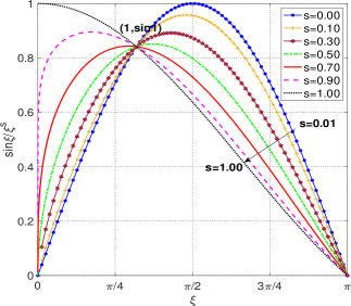
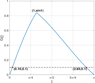
where for One verifies readily that attains its unique maximum value at where satisfies Moreover, for we have
On the other hand, for fixed (resp. ), is monotonically increasing (resp. decreasing) in so we have
| (3.22) |
and (see Figure 3.1). Thus we deduce from the intermediate value theorem that for any
| (3.23) |
Using (3.23) with and we find from (3.18), (3.19) and (3.21) that
| (3.24) |
which completes the proof. ∎
Remark 3.2.
In what follows, we analyze the stability and regularity of the flow map
| (3.25) |
It is noteworthy that in the splitting scheme, the logarithmic function is composited with trigonometric functions, and interestingly, has a higher regularity than the Hölder continuity of in the (non-regularised) implicit or semi-implicit schemes (see [29, 32]).
Theorem 3.2.
We have the following properties of the flow map
-
(i)
For any we have
(3.26) which implies if is Lipschitz continuous, so is
- (ii)
-
(iii)
For any we have
(3.28)
Proof.
Remark 3.3.
4. Low regularity analysis of the full-discretization scheme
In this section, we conduct rigorous error analysis for the Lie-Trotter time-splitting scheme (3.13) with spatial discretisation by the Fourier spectral method for the LogSE with low regularity solution in the fractional Sobolev space.
4.1. Full-discretization scheme
Notice from (3.12b) that if is periodic, then is periodic as well. We discretize (3.13) in space by the Fourier spectral method. Define
| (4.1) |
Let be the -orthogonal projection of on that is,
| (4.2) |
The Lie-Trotter time-splitting Fourier spectral (LTSFS) scheme for the LogSE (1.1) is to find recursively via
| (4.3) |
More precisely, we can obtain from by
| (4.4) |
where
| (4.5) |
Here the expansion coefficients in (4.5) will be computed very accurately via numerical quadrature with negligible quadrature errors. In fact, we find the use of over-quadrature (i.e., with the number of nodes more than ) appears necessary for such a nonlinear term with low regularity. Moreover, this is a relatively simpler setting for the clarity of analysis focusing on the logarithmic nonlinearity.
Note that is well-defined at (), although its first-order derivative about does not exist at . Then we shall. The first one is The sub-problem (3.11a) can be integrated in time and its solution is of the form The second is to solve As with the splitting scheme for the Schrödinger equation with cubic nonlinearity, the nonlinear sub-problem (3.11b) can be solved analytically with the solution
Some observations and remarks are in order.
-
(i)
Different from [Bao2019NM], the splitting step is not regularised. Here we understand if for some Accordingly, the composite function is continuous if is continuous.
-
(ii)
If with and , then
(4.6) see [Bao2019NM, Lemma 1] (where the regularized version of is valid for the non-regularized one in the second identity). Hence the splitting scheme is mass-preserving, i.e.,
-
(iii)
B
4.2. Useful lemmas
We make necessary preparations for the error analysis. We first derive some estimates for the nonlinear functions
| (4.7) |
which are useful to deal with the logarithmic nonlinear term. Such results will play an important role similar to the Cazenave-Haraux (CH) property of (cf. [18, Lemma 1.1.1]):
| (4.8) |
Lemma 4.1.
For any and we have
| (4.9a) | |||
| (4.9b) | |||
| (4.9c) | |||
where
Proof.
In fact, we can find (4.9a) from [29, Lemma 2.1]. For completeness, we provide a slightly different proof. It is trivial for . For , using the basic inequality: , we derive
With the aid of Lemma 4.1, we can derive the following important results valid on general bounded domain including .
Lemma 4.2.
For any and we have
| (4.11a) | |||
| (4.11b) | |||
where
| (4.12) |
Proof.
We first prove (4.11a). By (4.9b),
| (4.13) |
where We can show that for any and
| (4.14) |
Indeed, it is clear that if then the modulus of the logarithmic function is decreasing, so we have On the other hand, if it is increasing, so Thus, the first inequality in (4.14) holds. Using the same argument, we deduce that
Therefore, (4.14) is verified. Then we can derive (4.11a) from (4.13)-(4.14) straightforwardly.
In the error analysis, we also need to use the following stability result in the fractional periodic Sobolev space.
Lemma 4.3.
If with , then for
| (4.15) |
where
| (4.16) |
and for and for respectively.
Proof.
For , we derive from (4.14) directly that
For , we find from (4.9b) in Lemma 4.1 that
where . Then using Lemma 3.1 and (4.14), we derive that
| (4.17) |
Finally, for , we obtain from the direct calculation that
Since , we get from (4.14) that
This completes the proof. ∎
Finally, we present an inverse inequality and a relevant approximation result on Fourier expansions. It is noteworthy that they can be obtained from the the corresponding results in one dimension. Here we sketch the derivations in the Appendix for the readers’ reference, and the focus is placed on deriving sharper constants. Indeed, the -dimensional Fourier approximation can be founded in e.g., [30, Theorem 3.1] but with an implicit constant.
Lemma 4.4.
For any with , we have
| (4.18) |
Lemma 4.5.
For any with we have
| (4.19a) | |||
| (4.19b) | |||
where for or we understand
We shall show the unconditional -norm stability of the numerical solution obtained by the LTSFS method.
Lemma 4.6 (-stability).
Let and be defined in (4.3). Then for all , we have
| (4.20) |
Proof.
If or , the inequality (4.20) holds trivially. Noticing that, in norm, is bounded and is a linear isometry, we have
| (4.21) | ||||
Assuming and inserting a term , we can deduce that
| (4.22) | ||||
where we used the inequality for . In an analogue way, we can also obtain (4.22) if . Combining (4.21) and (4.22), we can obtain the desired result (4.20). ∎
4.3. Main result on error estimate
With the above preparations, we are now ready to carry out the convergence analysis of the Lie-Trotter splitting Fourier spectral method (4.3). For notational convenience, we denote
| (4.23) |
and
| (4.24) |
The main result is stated as follows.
Theorem 4.1.
Proof.
Using the triangle inequality and Lemma 4.5, we deduce that
| (4.27) |
Thus, it suffices to estimate From (4.3), we know that so
As the flow map of the linear Schrödinger’s operator satisfies and we derive from Theorem 3.2-(iii) the recurrence relation
which implies
| (4.28) | ||||
where we have noted Thus, by (4.27)-(4.28),
| (4.29) |
The rest of the proof is to show that for
| (4.30) |
Indeed, if (4.30) were proved, we obtain from (4.29) straightforwardly that
Since
Proof of (4.30). Let be the flow map of (1.1) with the initial value , that is,
| (4.31) |
Note that at . For simplicity of notation, we further introduce
| (4.32) |
As a direct projection of (4.31) leads to
| (4.33) |
We next derive the error equation of Using the definitions of in the scheme (4.3) and in (3.12a)-(3.12b), direct calculation leads to
where have used the simple fact It immediately implies
| (4.34) |
with . Accordingly, we derive from (4.33)-(4.34) the error equation:
| (4.35) |
In view of we notice that
| (4.36) |
so we next prove satisfying the estimate (4.30). For this purpose, taking the inner product with on the first equation of (4.35), the imaginary part of the resulting equation reads
| (4.37) |
As we use (4.8) to deal with the second term and get
which immediately implies
| (4.38) |
Using the Cauchy-Schwarz inequality, we obtain from (4.37)-(4.38) that
| (4.39) |
so it is necessary to estimate the two “error terms”: for , before we apply the Grönwall’s inequality to (4.39).
(i) Estimate . Using the triangle inequality, we further split into the following four terms:
| (4.40) |
where
| (4.41) |
We first estimate . Let be the identity operator. Using the theorems and lemmas stated previously, we can obtain
| (4.42) | ||||||
where and
We now estimate We observe from (4.3)-(4.4) that . Using the inverse inequality (4.18) and the facts: and we obtain from Lemma 4.5 and the conservation of mass: that
| (4.43) | ||||
and similarly,
| (4.44) |
Then we derive from the above that
| (4.45) |
Thus, we obtain from (4.42) and the above estimates that for
| (4.46) | ||||
Here, we use to denote a generic positive constant independent of and any function, and its dependence on other parameters (e.g., ) can be tracked if necessary. Note that we do not carry the factor which actually can be bounded by when we integrate
We now deal with given in (4.41). Following the derivations in (4.42), we can obtain
| (4.47) | ||||||
where
| (4.48) |
From the definition (3.12b) and the inverse inequality (4.18), we find readily that
| (4.49) |
Thus using (4.44), we can bound as with (4.45), and derive the following bound similar to (4.46):
| (4.50) |
We next turn to estimate in (4.41). Using the triangle inequality and aforementioned lemmas and theorem, leads to
| (4.51) |
where by (4.49),
| (4.52) | ||||
Thus, similar to (4.50), we have
| (4.53) |
Finally, we estimate in (4.41). From the property: we immediately derive Thus, we have
| (4.54) | ||||
where we denoted and in the last step, we used (4.9a) in Lemma 4.1. Using Theorem 3.1 and Lemma 4.5 and following the last three steps in (4.51), we obtain
Consequently, we have
| (4.55) |
A combination of the estimates of for in (4.46), (4.50), (4.53) and (4.55), leads to the bound for in (4.40), that is,
| (4.56) |
(ii) Estimate By the triangle inequality,
where as defined in (4.32). Using the property and Lemma 4.1, we can bound the first term by
We further bound the second term by using Lemma 4.3 and Lemma 4.5 as follows
where we noticed from (4.31) that so
The third term can be bounded by Lemma 4.2 and Lemma 4.5:
where by the inverse inequality (4.18), (4.14) and ,
Thus, we deduce from the above that
| (4.57) |
As a consequence of the regularity result in [15, Theorem 1.1] and Theorem 4.1, we have the following estimate for one-dimensional case.
Corollary 4.1.
If for some then we have the -estimate
| (4.59) |
for where is a positive constant. For we have a similar estimate if the solution
5. Error estimate for
In Theorem 4.1, we analyzed the convergence of the LTSFS scheme (4.3) when and the solution to (1.1) has certain fractional Sobolev regularity. Remarkably, it was shown that if the solution (see [15, Theorem 2.3] and (ii) in the introductory section). A natural question that arises is whether we can improve the -estimate (4.26) in Theorem 4.1 for to given the higher regularity. However, this cannot be obtained from the limiting process and the main reason that the limit cannot pass is (see Remark 3.3) and . Correspondingly, some results used for the proof of Theorem 4.1 are not valid for (e.g., (3.27)). We next take an alternative path to bypass the non-differentiability of and
Proof.
We first prove (5.4). If , the inequality in (5.4) holds trivially. If , by direct computation, we get
where for the last inequality we used for .
Then we turn to verify (LABEL:RPhiBstab). By direct calculation, we get
which gives immediately, since ,
| (5.1) | ||||
The proof ends. ∎
Theorem 5.1.
Proof.
The proof follows the same line as that of Theorem 4.1, but needs care to deal with the derivations involving and Indeed, following the steps in the proof of Theorem 4.1, we find the first one is in the second line of (4.42), so we bound the following term in differently as follows
| (5.3) |
where the regularised We can verify readily that
| (5.4) |
which is trivial for and for
so we can get (5.4) using for . Moreover, we need to use the property:
| (5.5) |
which follows directly from (see (3.32))
and the fact With these two intermediate results, we can now estimate the two terms in (5.3):
It is seen that the key is to shift the differentiation to the regularized with an extra -term. Then the estimate of in (4.46) becomes
| (5.6) |
The same issue happens to , i.e., the second line of (4.47). Using Lemma 4.5 and (5.4)-(5.5) again, we can obtain
With this change, we can update the bound of in (4.50) as
| (5.7) |
The situation with is slightly different, where appears in so we follow the same argument by inserting More precisely, we extract from (4.51) the following term and use Lemma 4.5, Lemma 4.2 and (5.4)-(5.5) to derive
where we noted . Thus, (4.53) is valid for that is,
| (5.8) |
Similarly, we re-estimate the following term in (see (4.54)) by using Theorem 3.1, Lemma 4.2 and (5.4)-(5.5) as follows
so (4.55) holds for namely,
| (5.9) |
Consequently, we obtain from (5.6)-(5.9) that
| (5.10) |
It is important to notice that the estimate of only involves the regularity of the solution In other words, the bound of in (4.57) is valid for .
Thanks to Theorem 5.1 and the regularity result in [15, Theorem 2.3] (also see (ii) in the introductory section), we have the following one-dimensional estimate similar to that in Corollary 4.1.
Corollary 5.1.
If then we have the -estimate
| (5.11) |
for where is a positive constant. For we have a similar estimate if the solution
6. Numerical results
In this section, we provide ample numerical results to validate the convergence of the LTSFS scheme (4.3) for solving the LogSE (1.1) with low regularity initial data. Given the nature of singularity, we find it is without loss of generality to test on the method in one spatial dimension.
6.1. Accuracy test on exact Gausson solutions
It is known that the LogSE has exact soliton-like Gausson solutions (see [9] and [2, (1.7)]):
| (6.1) |
where , and , are free to choose. Then we take the initial input to be
| (6.2) |
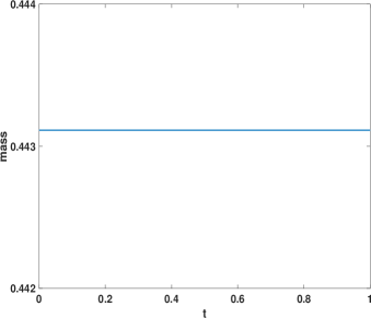
In the following tests, we take , , and set the interval of computation to be so that to enforce the periodic conditions. To demonstrate the convergence order in time, we use Fourier modes so that the error is dominated in time. In Figure 6.1, we plot on the left the -errors at against the time-stepping sizes of from to , and depict on the right time evolution of the mass. We observe from Figure 6.1 a perfect first-order convergence and a good conservation of the initial mass. Note that the solution (6.1) is sufficiently smooth, and
which implies and are smooth. On the other hand, we infer from Theorem 3.1 that the splitting scheme is first-order under -regularity. We believe the first-order convergence is attributed to these two facts, though the rigorous justification appears subtle. In addition, under the -regularity, Bao et al [3, Remark 2] showed the convergence order of the time-splitting scheme for the regularised LogSE. Then taking leads to the convergence order for any However, a similar estimate for the non-regularised case is not available which appears open.

6.2. Low regularity initial data for some
To verify the fractional-order convergence behaviours, we consider the following two examples.
Example 1: generated by decaying random Fourier coefficients. We construct through properly decaying Fourier expansion coefficients given by
| (6.3) |
where with real and imaginary parts being uniformly distributed random numbers on We find from the definition (3.3) that if then since
In real implementation, we truncate the infinite series with a cut-off number and randomly generate
where “rand( )” is the Matlab routine to produce a random vector drawn from the uniform distribution in the interval
In this case, the exact solution is unavailable, so we use the LTSFS scheme with
| (6.4) |
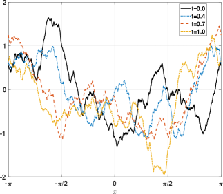
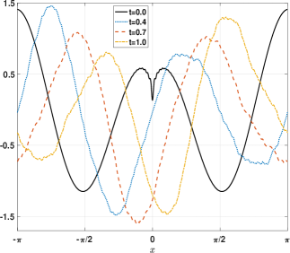
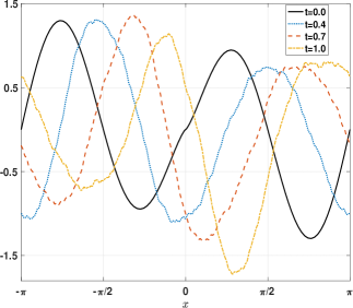
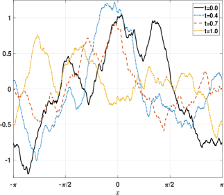
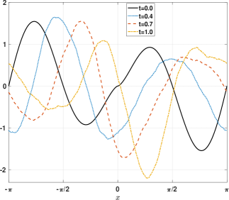
to compute a reference “exact” solution, denoted by at In Figure 6.2 (a)-(b), we plot the real and imaginary parts of and at on the left and right, respectively, for and Observe that the initial value and the reference solutions at different time are apparently continuous but not differentiable.
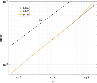
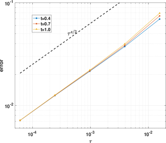
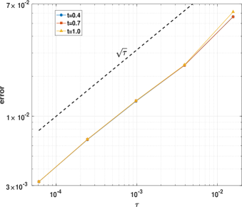
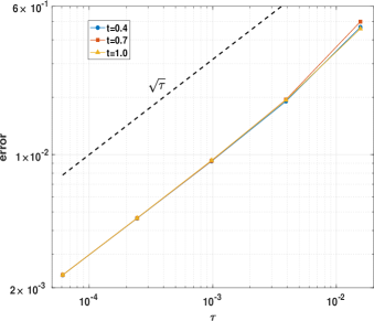
We now examine the error
| (6.5) |
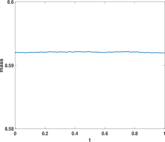
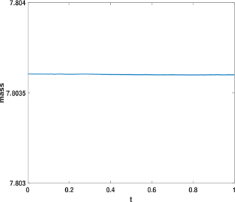
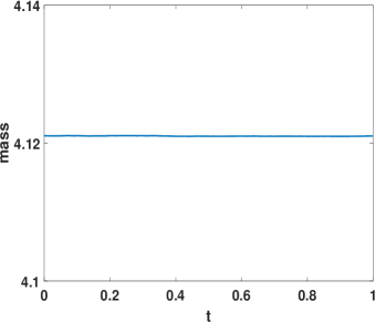
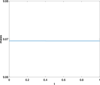
with the error bound predicted by Theorem 4.1 and Corollary 4.1, where we take and the constant depends on In Figure 6.2 (c), we plot the convergence in which roughly indicates the order as expected. It also shows the scheme is stable as the errors do not increase with time. We record the time evolution of mass in Figure 6.2 (d), which shows a good preservation of this quantity.
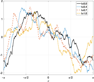
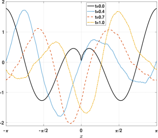
Example 2: Singular initial data To further validate the fractional order convergence, we consider (1.1) with the following singular initial data:
| (6.6) |
for some From the Taylor expansion of , we know the leading singularity of is Note that is -Hölder continuous in the sense that (see [20, pp 3-4]). Moreover, we find from the definition (3.5) and direct calculation that
| (6.7) | ||||
which is finite if and implies for sufficiently small It is noteworthy that Liu et al [25] introduced an optimal fractional Sobolev space characterised by the Riemann-Liouville fractional derivative and showed the regularity index without In addition, it seems subtle to show under the -periodic extension, though this regularity can be testified to by the numerical evidences below.
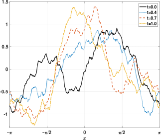
Here, we compute the reference solution with singular given in (6.6) (where ) and using the LTSFS with the discretisation parameters given in (6.4). The curves of the reference solutions at different time are depicted in Figure 6.3 (a)-(b). The error plot in Figure 6.3 (c) clearly indicates an (with ) convergence which agrees well with the prediction in Theorem 4.1 and Corollary 4.1. The evolution of mass recorded in Figure 6.3 (d) shows a good conservation of mass.
6.3. -initial data
To demonstrate the convergence behavior in Theorem 5.1 and Corollary 5.1, we take by letting in Example 1 and in Example 2.
Example 3: constructed by Example 1 with . We choose in (6.3) with , and follow the same setting as the previous subsection, but with Correspondingly, the reference solutions are depicted in Figure 6.4 (a)-(b), and the convergence and mass conservation are demonstrated in Figure 6.4 (c)-(d). We reiterate that we observe a perfect agreement of convergence order as in Theorem 5.1 and Corollary 5.1. We remark that Bao et al [3] also constructed low-regularity through random coefficients with a specified decaying rate, where -regularity was tested. Here, our construction is more straightforward with a better description of the decay, so the curve of convergence has a much better fitting of the predicted order.
Example 4: in Example 2 with . Here we set and in (6.6). In Figure 6.5, we show the curves of reference solution at , and demonstrate convergence rate in time and conservation of mass. Again, we observe a good agreement with the prediction.
7. Concluding remarks and discussions
While we are finalizing this work, we realize that Carles et al [15] showed the fractional Sobolev regularity of the LogSE on and where the use of fractional Sobolev norm in Bnyi and Oh [7, Proposition 1.3] (see Lemma 3.1) was indispensable to the analysis therein. Coincidentally, it is crucial in this context too. Here we also require the interplay between frequency and physical domain definitions, as seen in the proofs of the main results.
There appears a marginal gap between the regularity theory in [15, 22] and regularity requirements in Theorem 4.1 and Theorem 5.1, which additionally need (i.e., is bounded, though it is a sufficient condition). As a result, we could claim the convergence orders in Corollary 4.1 and Corollary 5.1 for from the regularity results in [15, 22] on the initial data . However, if then it is ensured as (see e.g., [2]).
We reiterate that different from the existing works, we analyze for the first time the low regularity fractional order convergence for the non-regularised splitting scheme. We also point out that we observe from numerical evidences the first-order convergence when but the rigorous proof appears open.
Appendix A Proof of Lemma 4.4
For any , we write
where is the -dimensional Dirichlet kernel
Then we obtain from the Cauchy-Schwarz inequality that
By the orthogonality of on , we have
Then we obtain (4.18) directly.
Appendix B Proof of Lemma 4.5
By the Parsval’s identity, we have
The second estimate can be obtained straightforwardly since
This ends the proof.
References
- [1] A.V. Avdeenkov and K.G. Zloshchastiev. Quantum Bose liquids with logarithmic nonlinearity: Self-sustainability and emergence of spatial extent. J. Phys. B-At. Mol. Opt., 44(19):195303, 2011.
- [2] W.Z. Bao, R. Carles, C.M. Su, and Q.L. Tang. Error estimates of a regularized finite difference method for the logarithmic Schrödinger equation. SIAM J. Numer. Anal., 57(2):657–680, 2019.
- [3] W.Z. Bao, R. Carles, C.M. Su, and Q.L. Tang. Regularized numerical methods for the logarithmic Schrödinger equation. Numer. Math., 143(2):461–487, 2019.
- [4] W.Z. Bao, R. Carles, C.M. Su, and Q.L. Tang. Error estimates of local energy regularization for the logarithmic Schrödinger equation. Math. Models Methods Appl. Sci., 32(1):101–136, 2022.
- [5] W.Z. Bao and C.S. Wang. Error estimates of the time-splitting methods for the nonlinear Schrödinger equation with semi-smooth nonlinearity. To appear in Math. Comp., 2023.
- [6] W.Z. Bao and C.S. Wang. Optimal error bounds on the exponential wave integrator for the nonlinear Schrödinger equation with low regularity potential and nonlinearity. To appear in SIAM J. Numer. Anal., 2023.
- [7] A. Benyi and T. Oh. The Sobolev inequality on the torus revisited. Publ. Math. Debrecen, 83(3):359–374, 2013.
- [8] I. Białynicki-Birula and J. Mycielski. Nonlinear wave mechanics. Ann. Physics, 100(1-2):62–93, 1976.
- [9] I. Białynicki-Birula and J. Mycielski. Gaussons: solitons of the logarithmic Schrödinger equation. Phys. Scripta, 20(3-4):539–544, 1979. Special issue on solitons in physics.
- [10] H. Buljan, A. Šiber, M. Soljačić, T. Schwartz, M. Segev, and D.N. Christodoulides. Incoherent white light solitons in logarithmically saturable noninstantaneous nonlinear media. Phys. Rev. E (3), 68(3):036607, 6, 2003.
- [11] J.C. Cao, B.Y. Li, and Y.P. Lin. A new second-order low-regularity integrator for the cubic nonlinear Schrödinger equation. IMA J. Numer. Anal., page drad017, 2023.
- [12] R. Carles. Logarithmic Schrödinger equation and isothermal fluids. EMS Surv. Math. Sci., 9(1):99–134, 2022.
- [13] R. Carles and G. Ferriere. Logarithmic Schrödinger equation with quadratic potential. Nonlinearity, 34(12):8283–8310, 2021.
- [14] R. Carles and I. Gallagher. Universal dynamics for the defocusing logarithmic Schrödinger equation. Duke Math. J., 167(9):1761–1801, 2018.
- [15] R. Carles, M. Hayashi, and T. Ozawa. Low regularity solutions to the logarithmic Schrödinger equation, 2023. arXiv:2311.01801 [math].
- [16] R. Carles and C.M. Su. Nonuniqueness and nonlinear instability of Gaussons under repulsive harmonic potential. Commun. Partial. Differ. Equ., 47(6):1176–1192, 2022.
- [17] R. Carles and C.M. Su. Numerical study of the logarithmic Schrödinger equation with repulsive harmonic potential. Discrete Contin. Dyn. Syst. - B, 28(5):3136–3159, 2023.
- [18] T. Cazenave and A. Haraux. Équations d’évolution avec non linéarité logarithmique. Ann. Fac. Sci. Toulouse Math., 5e série, 2(1):21–51, 1980.
- [19] F. Demengel and G. Demengel. Fractional Sobolev Spaces. Springer, London, 2012.
- [20] R. Fiorenza. Hölder and locally Hölder Continuous Functions, and Open Sets of Class , . Frontiers in Mathematics. Springer International Publishing, Cham, 2016.
- [21] T. Hansson, D. Anderson, and M. Lisak. Propagation of partially coherent solitons in saturable logarithmic media: A comparative analysis. Phys. Rev. A., 80(3):033819, 2009.
- [22] M. Hayashi and T. Ozawa. The Cauchy problem for the logarithmic Schrödinger equation revisited, 2023. arXiv:2309.01695 [math].
- [23] E.F. Hefter. Application of the nonlinear Schrödinger equation with a logarithmic inhomogeneous term to nuclear physics. Phys. Rev. A., 32(2):1201, 1985.
- [24] W. Królikowski, D. Edmundson, and O. Bang. Unified model for partially coherent solitons in logarithmically nonlinear media. Phys. Rev. E, 61(3):3122, 2000.
- [25] W.J. Liu, L.-L. Wang, and H.Y. Li. Optimal error estimates for Chebyshev approximations of functions with limited regularity in fractional Sobolev-type spaces. Math. Comp., 88(320):2857–2895, 2019.
- [26] S.D. Martino, M. Falanga, C. Godano, and G. Lauro. Logarithmic Schrödinger-like equation as a model for magma transport. EPL (Europhysics Letters), 63(3):472, 2003.
- [27] A. Ostermann, F. Rousset, and K. Schratz. Fourier integrator for periodic NLS: Low regularity estimates via discrete Bourgain spaces. J. Eur. Math. Soc., 25(10):3913–3952, 2022.
- [28] A. Ostermann and K. Schratz. Low regularity exponential-type integrators for semilinear Schrödinger equations. Found. Comput. Math., 18(3):731–755, 2018.
- [29] P. Paraschis and G. E. Zouraris. On the convergence of the Crank-Nicolson method for the logarithmic Schrödinger equation. Discrete Contin. Dyn. Syst. - B, 28:245–261, 2023.
- [30] L. Pareschi and T. Rey. Moment preserving Fourier–Galerkin spectral methods and application to the Boltzmann equation. SIAM J. Numer. Anal., 60(6):3216–3240, 2022.
- [31] J. Shen, T. Tang, and L.-L. Wang. Spectral Methods: Algorithms, Analysis and Applications. Springer-Verlag, New York, 2011.
- [32] L.-L. Wang, J.Y. Yan, and X.L. Zhang. Error analysis of a first-order IMEX scheme for the logarithmic Schrödinger equation. To appear in SIAM J. Numer. Anal., 2023.
- [33] K.G. Zloshchastiev. Logarithmic nonlinearity in theories of quantum gravity: Origin of time and observational consequences. Gravit. Cosmol., 16(4):288–297, 2010.