DEM: A Method for Certifying Deep Neural Network Classifier Outputs in Aerospace

Abstract

Software development in the aerospace domain requires adhering to strict, high-quality standards. While there exist regulatory guidelines for commercial software in this domain (e.g., ARP-4754 and DO-178), these do not apply to software with deep neural network (DNN) components. Consequently, it is unclear how to allow aerospace systems to benefit from the deep learning revolution. Our work here seeks to address this challenge with a novel, output-centric approach for DNN certification. Our method employs statistical verification techniques, and has the key advantage of being able to flag specific inputs for which the DNN’s output may be unreliable — so that they may be later inspected by a human expert. To achieve this, our method conducts a statistical analysis of the DNN’s predictions for other, nearby inputs, in order to detect inconsistencies. This is in contrast to existing techniques, which typically attempt to certify the entire DNN, as opposed to individual outputs. Our method uses the DNN as a black-box, and makes no assumptions about its topology. We hope that this work constitutes another step towards integrating DNNs in safety-critical applications — especially in the aerospace domain, where high standards of quality and reliability are crucial.

1 Intoduction

Air transportation handles billions of passengers annually, and requires advanced solutions for addressing longstanding efficiency, environmental impact, and safety challenges [8]. The deep learning revolution, and specifically deep neural networks (DNNs), show great potential for addressing this need [28, 34]. However, although DNNs have demonstrated remarkable performance, they remain susceptible to tiny perturbations in their inputs, which may result in misclassification. This vulnerability, referred to as adversarial inputs [12, 15], could trigger a chain of events that would result in serious injury, extensive damage to valuable assets, and irreparable damage to delicate ecosystems [17]. Consequently, adversarial inputs are a key limitation that is preventing DNNs from being integrated into safety-critical systems.

In the aerospace industry, certification authorities such as the European Aviation Safety Agency (EASA) and the Federal Aviation Administration (FAA) play a key role in advocating for civil aviation safety and environmental preservation. These authoritative bodies acknowledge the immense value of incorporating DNNs into safety-critical applications [8], yet also emphasize that conventional software certification guidelines, such as DO-178 [10], are not applicable to DNNs. In recognition of the inherent challenges of certifying DNNs within the aerospace domain, EASA recently released its comprehensive AI roadmap [8], which outlines seven pivotal requirements for ensuring artificial intelligence trustworthiness. Of these, robustness to adversarial conditions is mentioned as one of the fundamental prerequisites. Thus, it is evident that ensuring a DNN’s robustness to adversarial inputs will play an important role in any future certification process.

During the preliminary stage of an aerospace certification process, the FAA ARP-4754 guidelines [9] call for conducting a safety analysis procedure for all aircraft systems and subsystems. For each subsystem, the safety engineering team is required to determine the permissible probability of failure, with which the design engineer then has to comply. In order to carry out such a process for a system that incorporates a DNN, the engineering team must demonstrate that the probability of a failure related to the DNN does not exceed the threshold established in the safety analysis. Unfortunately, there is currently a shortage of techniques for performing this analysis that are both sufficiently precise and scalable.

Here, we seek to bridge this crucial gap by introducing a novel DNN certification approach, DNN Enable Monitor (DEM). Inspired by wireless network management concepts [20, 2], instead of trying to certify the DNN as a whole, DEM focuses on certifying only the DNN’s outputs. For each output of the DNN, DEM calculates, on-the-fly, the probability of misclassification — and if this probability is below a certain acceptable threshold, the output is considered certified. Otherwise, the output is flagged and passed on for further analysis, e.g., by a human expert. The motivation here is that well-trained DNNs, working under normal conditions, are generally correct; and so identifying the few cases where the DNN might be wrong and further analyzing only these cases can relieve a significant cognitive load off the human experts, compared to a manual approach. Further, if the automated certification is accurate enough, then the entire process becomes nearly fully automatic — and also sufficiently accurate to meet the bars specified in the safety analysis phase.

Internally, DEM applies the following principle in order to determine whether an output produced by the DNN is correct or not. Consider an input $\vec{x_{0}}$, which is mapped by the DNN to label $l_{0}$. If this classification is correct, then it stands to reason that most input points very close to $\vec{x_{0}}$ would also be classified as $l_{0}$. If, however, $\vec{x_{0}}$ is an adversarial input, which can intuitively be interpreted as a “glitch” in the DNN, then other points around $\vec{x_{0}}$ would be classified differently. The purpose of DEM is to effectively distinguish between these two cases.

In order to achieve this, DEM leverages the recently proposed concept of probabilistic global categorial robustness, presented as part of the gRoMA method for statistically evaluating the global robustness of a classifer DNN, per output category [22]. The gRoMA approach is scalable, and does not require any assumptions about the DNN itself: the DNN is treated as a black-box, and the method does not depend on its activation functions, parameters, hyper-parameters, or internal topology. These advantages carry over to DEM as well. However, while gRoMA focuses strictly on measuring a DNN’s global robustness, DEM extends this approach to determine whether a particular output of the DNN should be considered certified or not.

For evaluation purposes, we created a proof-of-concept implementation of DEM, and used it to evaluate VGG16 [29] and Resnet [13] DNN models. Our evaluation shows that DEM outperforms state-of-the-art methods in adversarial input detection, and that it successfully distinguishes adversarial inputs from genuine inputs — with up to 100% success rate in some categories, which is of course sufficiently high to meet the aerospace regulatory requirements.

A major advantage of DEM is that it computes different thresholds for certifying outputs for the different classifier categories — making it flexible and accurate enough to handle cases where it is impossible to select a uniform threshold for all output categories. To the best of our knowledge, this is the first effort at certifying the categorial robustness of DNN outputs, for safety-critical DNNs.

The rest of the paper is organized as follows. We begin in Sec. 2 with a description of prior work, and then present the required background on adversarial robustness in Sec. 3. We then describe our proposed method for measuring adversarial robustness in Sec. 4, followed by a description of our evaluation in Sec. 5. Finally, we summarize and discuss our results in Sec. 6.

2 Related Work

The certification of DNNs and their integration into safety-critical applications has been the subject of extensive research [11, 7, 5]. In general, DNN certification rests on two main foundations: certification guidelines and DNN robustness.

Certification Guidelines. A widely accepted cornerstone in system and software certification within the aerospace domain is the “ARP-4754 — Guidelines for Development of Civil Aircraft Systems and Equipment Certification” guidelines [9]. These guidelines were authored by SAE International, a global association of aerospace engineers and technical experts. The guidelines focus on safety considerations when developing civil aircraft and their associated systems. However, these guidelines do not directly apply to DNN components.

A recent work [14] proposed an approach for assessing DNN robustness using an alternative Functional Hazard Analysis (FHA) method. This method is similar to the one required by ARP-4754, but does not quite address the requirements in the guidelines.

Another recent study [11] developed a comprehensive framework of principles for DNN certification, which is aligned with ARP-4754 — but which does not include a concrete method or tool that can be used.

While ARP-4754 focuses on system level certification, the influential DO-178 guidelines for airborne systems focus on software certification [10]. These guidelines define 5 levels (A-E) for software failure conditions. Initial work has discussed certifying DNNs to level D [5, 6] or C [4, 7, 4], but to date none have reached Level A — the most severe level, required where failures may lead to fatalities, which is the case in aerospace. We hope that our approach can be used to satisfy Level A requirements in the future.

DNN Robustness. An alternative approach to the one proposed here, which has received significant attention, is the formal certification of DNN robustness. The idea is to conclude, a-priori, that a DNN is safe to use, at least for certain regions of its input space.

One approach for drawing such conclusions is to formally verify DNNs [15, 31]. DNN verification methods are highly accurate, but suffer from limited scalability, require white-box access to the DNN in question, and pose certain limitations on the DNN’s topology and activation functions.

Another approach attempts to circumvent these limitations by certifying a DNN’s robustness with significant margins of error [35, 33, 1, 14]. This kind of attempt may be inadequate for certification in aerospace, where large error margins are usually not acceptable.

Finally, there exist statistical approaches for evaluating the probability that a specific input is being misclassified by the network (i.e., is an adversarial input)  [32, 30, 25]. However, the performance of these approaches typically falls short of the level required by regulators. DEM is also statistical at its core, and we later show that it outperforms the state of the art significantly, leading us to hope that it could be applied in aerospace. Specifically, we compare DEM to LID [23], a state-of-the-art method in this category. As we later discuss, part of the advantage of our method over LID is that DEM can be configured to be conservative, i.e., to refrain from falsely declaring that an output is certified.

3 Background

Deep Neural Networks (DNNs). A deep neural network (DNN) $N$ is a function $N:\mathbb{R}^{n}\rightarrow\mathbb{R}^{m}$, which maps an input vector $\vec{x}\in\mathbb{R}^{n}$ to an output vector $\vec{y}\in\mathbb{R}^{m}$. In this paper we focus on classification DNNs, where $\vec{x}$ is classified as class $c$ if the $c$’th entry of $N(\vec{x})$ has the highest score: $\operatorname*{arg\,max}(N(\vec{x}))=c$.

Local Adversarial Robustness. Local adversarial robustness is a measure of how resilient a DNN is to perturbations around specific input points [3]:

Definition 1

A DNN $N$ is $\epsilon$-locally-robust at input point $\vec{x_{0}}$ iff

$$\forall\vec{x}.\displaystyle||\vec{x}-\vec{x_{0}}||_{\infty}\leq\epsilon\Rightarrow\operatorname*{arg\,max}(N(\vec{x}))=\operatorname*{arg\,max}(N(\vec{x_{0}}))$$

Intuitively, Definition 1 states that for input vector $\vec{x}$, the network assigns to $\vec{x}$ the same label that it assigns to $\vec{x_{0}}$, as long as the distance of $\vec{x_{0}}$ from $\vec{x}$ is at most $\epsilon$ (using the $L_{\infty}$ norm).

Probabilistic Local Robustness. Definition 1 is boolean: given $\epsilon$ and $\vec{x_{0}}$, the DNN is either robust or not robust. However, in real-world settings, and specifically in aerospace applications, systems could still be determined to be sufficiently robust if the likelihood of encountering adversarial inputs is greater than zero, but is sufficiently low. Federal agencies, for example, provide guidance that a likelihood for failure that does not exceed $10^{-9}$ (per operational hour under normal conditions) is acceptable [19]. Hence, we make an adjustment to Definition 1 that allows us to reason about a DNN’s robustness in terms of its probabilistic-local-robustness (plr) [21], which is a real value that indicates a DNN’s resilience to adversarial perturbations imposed on specific inputs. More formally:

Definition 2

The $\epsilon$-probabilistic-local-robustness (PLR) score of a DNN $N$ at input point $\vec{x_{0}}$, abbreviated $\text{plr}{}{}_{\delta,\epsilon}(N,\vec{x_{0}})$, is defined as:

$$\text{plr}{}{}_{\delta,\epsilon} (N,\vec{x_{0}})\triangleq P_{x:\lVert\vec{x}-\vec{x_{0}}\rVert_{\infty}\leq\epsilon}[(\operatorname*{arg\,max}(N(\vec{x}))=\operatorname*{arg\,max}(N(\vec{x_{0}})))]$$

Intuitively, the definition measures the probability that for an input $\vec{x_{0}}$, an input $\vec{x}$ drawn at random from the $\epsilon$-region around $\vec{x_{0}}$ will have the same label as $\vec{x_{0}}$.

Probability Global Caterorial Robustness (PGCR). Although Definition 2 is more realistic than Definition 1, it suffers from two drawbacks. The first: recent studies indicate a significant disparity in robustness among the output categories of a DNN [21, 22], which is extremely relevant to safety-critical applications. However, Definition 2 does not distinguish between output classes. The second drawback is that Definition 2 considers only local robustness, i.e., robustness around a single input point, in a potentially vast input space; whereas it may be more realistic to evaluate robustness on large, continuous chunks of the input space. To address these drawbacks, we use the following definition [22]:

Definition 3

Let $N$ be a DNN, let $l\in L$ be an output label. The ($\epsilon,\delta$)-PGCR score for $N$ with respect to $l$, denoted $pgcr_{\delta,\epsilon}(N,l)$, is defined as:

$$pgcr_{\delta,\epsilon}(N,l)\triangleq P_{\vec{x_{1}},\vec{x_{2}}\in\mathbb{R}^{n}||\vec{x_{1}}-\vec{x_{2}}||_{\infty}\leq\epsilon}[|N(\vec{x_{1}})[l]-N(\vec{x_{2}})[l]|<\delta]$$

This definition captures the probability that for an input $\vec{x_{1}}$, and for an input $\vec{x_{2}}$ that is at most $\epsilon$ apart from $\vec{x_{1}}$, the confidence scores for inputs $\vec{x_{1}}$ and $\vec{x_{2}}$ will differ by at most $\delta$ for the label $l$.

4 The Proposed Method

4.1 The Inference Phase

Given an input point $\vec{x}_{0}$, our objective is to quantify the reliability of the DNN’s particular prediction, $N(\vec{x}_{0})$. Our method for achieving this consists of the following steps:

• Execute the DNN on input $\vec{x}_{0}$, and obtain the prediction $N(\vec{x}_{0})$.

• Generate $k$ perturbations around $\vec{x}_{0}$, denoted $\vec{x}^{\prime}_{1}\ldots\vec{x}^{\prime}_{k}$, sampled uniformly at random from an $\epsilon$-region around $\vec{x}_{0}$.

• For each sampled perturbation point $\vec{x}_{i}^{\prime}$, compute the prediction $N(\vec{x}_{i}^{\prime})$ and check whether it coincides with $N(\vec{x}_{0})$. Count the number of such matches (“number of hits”), denoted $h$.

• If $h$ is above a certain threshold $\mathcal{T}$, certify the prediction of $N(\vec{x}_{0})$ as correct. Otherwise, flag it as suspicious.

The motivation for this approach is that, if $\vec{x}_{0}$’s prediction is genuine, the network should produce similar predictions for many points around $\vec{x}_{0}$; in which case, the number of hits will be high, and will exceed threshold $\mathcal{T}$. Conversely, if $\vec{x}_{0}$’s prediction is not genuine, i.e. $\vec{x}_{0}$ is an adversarial input for $N$, then there will be many points around $\vec{x}_{0}$ that are classified correctly — and consequently, their classification differs from that of $\vec{x}_{0}$, and the number of hits will be low.

Naturally, in order for this approach to work great care must be taken in selecting the two key parameters: $\epsilon$, which determines the size of the region around $\vec{x}_{0}$ from which perturbations are sampled, and the threshold $\mathcal{T}$ for deciding whether a prediction is correct. Intuitively, selecting too large a value for $\epsilon$ will reduce the number of hits for genuine inputs, because the region will include inputs that have true different classifications; whereas selecting too small a value will result in a high number of hits also for adversarial inputs, due to the continuous nature of DNNs. To resolve this, we present next a method for selecting these values.

4.2 Dataset Preparation and Calibration

Our approach requires an offline calibration phase, to adjust the method’s parameters to the DNN at hand. Recall that, during inference, random samples are procured from an $\epsilon$-region around the input point $\vec{x}_{0}$; and that our goal is to select $\epsilon$ in such a way that many of these samples will be classified the same way as $\vec{x}_{0}$ when it is genuine, but only a few will meet this criterion when $\vec{x}_{0}$ is adversarial. As it turns out, different $\epsilon$ values can cause dramatic differences in the number of hits; see Fig. 1 for an illustration. In order to select an appropriate value of $\epsilon$, we use an empirical approach that leverages Levy et al.’s method for computing $PGCR$ values: we test multiple potential values of $\epsilon$, and select the one that produces the best result.

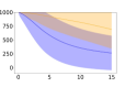
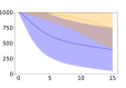
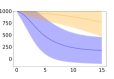
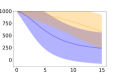
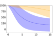
(a) Airplane, Automotive, Bird, Cat, Deer categories, respectively

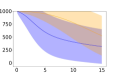
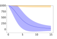
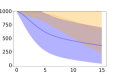
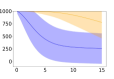
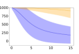
(b) Dog, Frog, Horse, Ship, Truck categories, respectively

Figure 1: An illustration of the performance of a CIFAR-10 classifier. Each graph corresponds to a single output category. The $Y$-axes in the graphs show the average number of hits (bold line) and standard deviation (faded area), for $k=1000$ perturbations around genuine (blue) and adversarial (orange) images; whereas the $X$-axes represent different values of $\epsilon$ (in percents). The goal is to have as little overlap as possible between the two shaded areas; and we observe that an intelligent choice of $\epsilon$ can make a huge difference.

Dataset Creation. First, we obtain a set of $n$ correctly classified (genuine) inputs from the test data, $X_{g}=\{\vec{x}^{g}_{1},\ldots,\vec{x}^{g}_{n}\}$. From this set, we construct a set $X_{a}=\{\vec{x}^{a}_{1},\ldots,\vec{x}^{a}_{m}\}$ of adversarial inputs, obtained from the points in $X_{g}$ by applying state-of-the-art attacks, such as PGD [24, 26]. We also consider a set of $\ell$ potential $\epsilon$ values, $E=\{\epsilon_{1},\ldots,\epsilon_{\ell}\}$, from among which we will select the $\epsilon$ value to be used during inference.

Next, for each $\epsilon\in E$ and for each input point $\vec{x}\in X=X_{g}\cup X_{a}$, we sample $k$ perturbed inputs $\vec{x}^{\prime}_{1}\ldots\vec{x}^{\prime}_{k}$ from the $L_{\infty}$ $\epsilon$-region around $\vec{x}$ [21, 22]. We then evaluate $N$ on $\vec{x}$ and on its perturbations $\vec{x}^{\prime}_{1}\ldots\vec{x}^{\prime}_{k}$, obtaining the outputs $N(\vec{x})$ for $\vec{x}$ and $N(\vec{x}^{\prime}_{1})\ldots N(\vec{x}^{\prime}_{n})$ for the perturbations. We count the number of hits, $h^{\vec{x}}_{\epsilon}=|\{i\ |\operatorname*{arg\,max}{N(\vec{x}^{\prime}_{i})}=\operatorname*{arg\,max}{N(\vec{x})}\}|$, and store it for later use.

We note that instead of using the measure of hits as a predictor for whether the input being examined is adversarial, one could try to discover the distribution of adversarial inputs, and then attempt to decide whether an input is likely to belong to that distribution. However, determining the distribution of adversarial inputs is difficult, and could not be achieved, empirically, using state-of-the-art statistical tools [27].

4.3 Maximal-Recall-Oriented Calibration

Using the collected data for various $\epsilon$ values, we present Alg. 1 for selecting an optimal value of $\epsilon$, and its corresponding threshold $\mathcal{T}$. The sought-after $\epsilon$ is optimal in the sense that, when used in the inference phase, it makes the fewest classification mistakes. The selection algorithm is brute-force: we consider each $\langle\epsilon,\mathcal{T}\rangle$ pair in turn, compute its success rate, and then pick the best pair.

The algorithm receives as input the set of potential $\epsilon$ values $E$; the sets of genuine and adversarial points, $X_{g}$ and $X_{a}$, respectively; the measured number of hits, $h^{\vec{x}}_{\epsilon}$, for each input point $\vec{x}$ and each $\epsilon$; and also the hyper-parameter $w_{g}$, discussed later. The algorithm’s outputs are the selected $\epsilon$ value, denoted $\epsilon^{*}$, and its corresponding threshold of hits, $\mathcal{T}$, to be used in the inference phase.

Algorithm 1 Maximal-Recall-Oriented Calibration

Input: $E$, $X_{g}$, $X_{a}$, $\{h^{\vec{x}}_{\epsilon}\}$, $w_{g}$
    Output: $\epsilon^{*},\mathcal{T}$

1:  $\epsilon^{*},bestScore,\mathcal{T}\leftarrow 0,0,0$

2:  for all $\epsilon\in E$ do

3:     for $t:=0\ldots k$ do

4:        $r_{g}=|\{\vec{x}\in X_{g}\ |\ h_{\epsilon}^{\vec{x}}>t\}|$ / $|X_{g}|$

5:        $r_{a}=|\{\vec{x}\in X_{a}\ |\ h_{\epsilon}^{\vec{x}}<t\}|$ / $|X_{a}|$

6:        $score=w_{g}\cdot r_{g}+(1-w_{g})\cdot r_{a}$

7:        if $score>bestScore$ then

8:           $\epsilon^{*}\leftarrow\epsilon,bestScore\leftarrow score,\mathcal{T}\leftarrow t$

9:        end if

10:     end for

11:  end for

12:  return  $\epsilon^{*},\mathcal{T}$

Line 2 constitutes the main loop of the algorithm, iterating over all potential values of $\epsilon$ in order to pick the best one. For each such $\epsilon$, we iterate over all possible threshold values in Line 3; since each $\langle\epsilon,\vec{x}\rangle$ pair was tested over $k$ perturbed inputs, the number of hits can be anywhere between $0$ and $k$, and we seek the best choice. Line 4 computes the fraction of genuine inputs for which the threshold was reached, whereas Line 5 computes the fraction of adversarial inputs for which the threshold was not reached; these values are called the recall rates, and are denoted $r_{g}$ and $r_{a}$, respectively. Then, Line 6 computes a real-valued score for this candidate $\epsilon$. The score is a weighted average between $r_{g}$ and $r_{a}$, where the hyper-parameter $w_{g}$ is used in prioritizing between a more conservative classification of inputs ($w_{g}$ is lower, leading to fewer adversarial inputs mistakenly classified as genuine), or a less conservative one. The best score, and its corresponding $\epsilon$ and threshold, are stored in Line 8; and the selected $\epsilon$ and threshold are returned in Line 12.

Note. Alg. 1 computes a single $\epsilon$ value to be used during inference. However, in practice we observed that the approach is more successful when different $\epsilon$ values are used for the different output classes (see Fig. 1). E.g., during inference, if the input at hand is classified as “dog”, one $\epsilon$ value is used; whereas if it classified as “cat”, another is selected. To make this adjustment, Alg. 1 needs to be run once for each output class, and the sets $X_{a}$ and $X_{g}$ need to be partitioned by output class, as well. For brevity, we omit these adjustments here, as well as in subsequent algorithms.

4.4 Maximal-Precision-Oriented Calibration

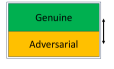
(a) Recall Calibration Goals

(b) Precision Calibration Goals

Figure 2: Different optimization goals: the recall-oriented algorithm seeks the optimal threshold value that maximizes the separation between genuine and adversarial instances. The precision-oriented algorithm strives to minimize the “yellow” area, by determining the lowest threshold that maximizes adversarial input detection and the highest threshold that maximizes genuine input detection, e.g., minimizing the “unknown” cases for both thresholds.

Alg. 1 is geared for recall; i.e., during inference, it classifies every input as either genuine (if the number of hits exceeds the threshold), or as suspected as adversarial. However, in our studies we observed that often, a division into three classes was more appropriate: in many cases, inputs encountered during inference would either demonstrate a very high number of hits, in which case they are likely genuine; a very low number of hits, in which case they are likely adversarial; or a medium number of hits, in which case it is unclear whether they are adversarial or not. Whereas in Alg. 1 a human would have to inspect all inputs suspected as adversarial, a more subtle division into there classes could allow the human to only inspect those inputs that are in the third, “unknown” category. See Fig. 2 for an illustration.

To support this variant, we present Alg. 2, which is geared for increased precision. It is similar to Alg. 1, but instead of selecting an $\epsilon$ and returning a single threshold $\mathcal{T}$, it now returns a couple of thresholds — $\mathcal{T}_{g}$ that indicates a lower bar of hits for genuine inputs, and $\mathcal{T}_{a}$ that indicates an upper bar of hits for adversarial inputs. When this algorithm is used, the final inference step is changed into:

• If $h$ is above a certain threshold $\mathcal{T}_{g}$, certify the prediction of $N(\vec{x}_{0})$ as correct. If $h$ is below a certain threshold $\mathcal{T}_{a}$, mark it as adversarial. Otherwise, flag it as “unknown”.

We observe that when using this three-output scheme, there is an inherent tension between precision and recall. For example, remembering that genuine inputs tend to have a high number of hits and adversarial inputs a low number, one could set $\mathcal{T}_{g}$ to be very high and $\mathcal{T}_{a}$ to be very low. This would result in excellent precision (i.e., the algorithm would make only few mistakes), but many inputs would fall in the “unknown” category, causing poor recall. In terms of Fig. 2, this would result in a very wide yellow strip. Alternatively, one could set these two thresholds to be near-identical (resulting in a narrow yellow strip), which would simply mimic Alg. 1, with its excellent recall but sub-optimal precision. To resolve this, we allow the user to specify a-priori the desired precision, by setting minimal values $p_{g}^{\min}$ and $p_{a}^{\min}$ for the precision over genuine and adversarial inputs, respectively. Our algorithm then automatically selects the $\epsilon$ and threshold values that meet these requirements, and which achieve the best recall among all candidates.

More concretely, the inputs to Alg. 2 are the same as those to Alg. 1, plus the two threshold parameters, $p_{g}^{\min}$ and $p_{a}^{\min}$. For each candidate $\epsilon$, the algorithm iterates over all possible thresholds (Line 4), from high to low, each time computing the recall rates (Lines 5–6) and the precision rate over genuine inputs (Line 7). If the precision rate meets the specified threshold, the threshold is stored as $t_{1}$ in Line 9. At the end of this loop, the algorithm has identified the lowest threshold for genuine inputs that meets the requirements. Next, the algorithm begins a symmetrical process for the threshold for adversarial inputs, this time iterating from low to high (Line 14), until it identifies the greatest threshold that satisfies the requirements ($t_{2}$, Line 19). Once both thresholds are discovered, the algorithm uses the recall ratios to compute a score (Line 24) — in order to compare the various $\epsilon$ values. The best $\epsilon$ and its thresholds are stored in Line 25, and are finally returned in Line 29.

Algorithm 2 Maximal-Precision-Oriented Calibration

Input: $E$, $X_{g}$, $X_{a}$, $\{h^{\vec{x}}_{\epsilon}\}$, $w_{g}$, $p_{g}^{\min}$, $p_{a}^{\min}$
    Output: $\epsilon^{*}$, $\mathcal{T}_{g}$,$\mathcal{T}_{a}$

1:  $\epsilon^{*},bestScore,\mathcal{T}_{g},\mathcal{T}_{a},r_{\mathcal{T}_{g}},r_{\mathcal{T}_{a}}\leftarrow 0,0,0,0,0,0$

2:  for all $\epsilon\in E$ do

3:     $r_{1},r_{2}\leftarrow 0,0$

4:     for $t:=k\ldots 1$ do

5:        $r_{g}=|\{\vec{x}\in X_{g}\ |\ h_{\epsilon}^{\vec{x}}>t\}|$ / $|X_{g}|$

6:        $r_{a}=|\{\vec{x}\in X_{a}\ |\ h_{\epsilon}^{\vec{x}}<t\}|$ / $|X_{a}|$

7:        $p_{g}=r_{g}/\left(r_{g}+(1-r_{a})\right)$

8:        if $p_{g}>p_{g}^{\min}$ then

9:           $t_{1}\leftarrow t$, $r_{1}\leftarrow r_{g}$

10:        else

11:           break

12:        end if

13:     end for

14:     for $t:=1\ldots t_{1}$ do

15:        $r_{g}=|\{\vec{x}\in X_{g}\ |\ h_{\epsilon}^{\vec{x}}>t\}|$ / $|X_{g}|$

16:        $r_{a}=|\{\vec{x}\in X_{a}\ |\ h_{\epsilon}^{\vec{x}}<t\}|$ / $|X_{a}|$

17:        $p_{a}=r_{a}/\left(r_{a}+(1-r_{g})\right)$

18:        if $p_{a}>p_{a}^{\min}$ then

19:           $t_{2}\leftarrow t$, $r_{2}\leftarrow r_{a}$

20:        else

21:           break

22:        end if

23:     end for

24:     $score=w_{g}\cdot r_{1}+(1-w_{g})\cdot r_{2}$

25:     if $(score>bestScore)$ then

26:        $\epsilon^{*}\leftarrow\epsilon,bestScore\leftarrow score,\mathcal{T}_{g}\leftarrow t_{1},\mathcal{T}_{a}\leftarrow t_{2}$

27:     end if

28:  end for

29:  return  $\epsilon^{*},\mathcal{T}_{g},\mathcal{T}_{a}$

5 Evaluation

Implementation. In order to evaluate our method, we created a proof-of-concept implementation of Algs. 1 and 2 in a tool called DEM, which is available online and will be made publicly available with the final version of this paper [16]. Our tool is written in Python, and supports DNNs in the common PyTorch format.

Baseline. In our experiments we compared the two algorithms within DEM (recall-oriented and precision-oriented), and also compared DEM’s recall-oriented algorithm to the Local Intrinsic Dimension (LID) method [23], which is the state-of-the-art detecting adversarial examples. Like DEM, LID has a calibration phase, in which the network is evaluated on multiple genuine and adversarial inputs. LID uses these evaluations to examine the assignments to the various neurons of the DNN, and then trains a regression model to predict, during inference and based on these values, whether an input is adversarial. Since LID was not originally designed for categorical data, we trained it using two separate methods: (i) using examples from all classes, as originally suggested [23]; and (ii) training ten LID detectors, one for each output class. The second approach improved LID’s performance slightly, and we used it in the experiments described next.

Benchmarks. We used VGG16 [29] and Resnet [13] DNN models, trained on the CIFAR10 dataset [18]. The Resnet and VGG models achieved $88.35\%$ and $83.75\%$ accuracy, respectively. We then took the CIFAR10 test set, removed from it any inputs that were misclassified by the trained models, and split the remaining inputs into two sets: a calibration set with $80\%$ of the inputs, and an evaluation set with the remaining $20\%$. The adversarial inputs for the calibration and evaluation phases were obtained using PGD [24], with a maximal modification distance of $0.005$ (i.e., $0.5\%$).

In the preliminary calibration phase, we created $1000$ perturbed inputs around each genuine and adversarial example. We empirically observed that $1000$ samples was a suitable choice sufficient — using additional inputs did not change our algorithm’s outputs significantly, whereas using significantly fewer inputs led to a less-accurate calibration. For both calibration methods, we set the genuine recall hyperparameter to $w_{g}=0.3$. This conservative choice prioritizes avoiding adversarial examples wrongly misclassified as genuine. For the set $E$ of candidate $\epsilon$ values, we arbitrarily used distance values ranging from $0.001$ to $0.15$, with $0.001$ resolution. While RoMA and gRoMA used an $\epsilon$ value of $0.04$, we decided to use a greater value to ensure we do not miss a better calibration value. We note again that large values of $\epsilon$ reduce the number of hits for genuine inputs, because the region includes legitimate inputs that have true different classifications; and we empirically found that a distance greater than $0.15$ typically causes this number to drop too steeply.

We conducted our evaluation on a standard laptop, equipped with an AMD Ryzen 9 6900HX CPU, an NVIDIA GeForce RTX 3070 GPU, and 16GB of RAM. In order to create a virtual running environment, we used Python 3.11 and PyTorch 2.11. The calibration and data preparation for each algorithm took less than four hours, per class. Each sample was analyzed in less than 0.003 seconds. The code for the creation of adversarial examples, calibration, and evaluation is available online [16].

5.1 Evaluating the Recall-Oriented Calibration Algorithm

Table 1 provides a comparison of our recall-oriented calibration algorithm with LID [23]. It demonstrates that the proposed method is highly effective at distinguishing between genuine and adversarial inputs. Compared to LID, we observe that LID identifies genuine examples with a slightly better recall; however, DEM is significantly better at identifying adversarial inputs significantly, for all classes. This is a favorable result, as the mistake of classifying an adversarial input as a genuine one is considered to be much more serious than the second kind of mistake — classifying a genuine input as an adversarial.

Table 1: Evaluating the recall-oriented calibration algorithm, in comparison to LID. The evaluation includes the Resnet (marked as RES) and VGG (marked as VGG) models. The two parts of the table present genuine and adversarial recall: the number of samples, the recall achieved by DEM, and the recall achieved by LID.

Class	Genuine Recall			Adversarial Recall
	#Samples RES|VGG	DEM	LID	#Samples RES|VGG	DEM	LID
Airplane	180|177	63%|76%	81%|88%	393|125	92%|86%	54%|30%
Automotive	190|185	65%|65%	80%|91%	290|80	94%|87%	43%|52%
Bird	169|160	79%|67%	80%|84%	441|159	91%|91%	44%|35%
Cat	149|146	51%|50%	74%|85%	547|246	91%|89%	52%|31%
Deer	179|176	80%|79%	76%|89%	526|186	93%|97%	47%|37%
Dog	164|135	56%|60%	74%|87%	465|183	91%|92%	44%|30%
Frog	183|174	99%|91%	76%|84%	452|138	99%|97%	54%|34%
Horse	183|174	65%|74%	84%|88%	404|125	88%|87%	44%|38%
Ship	188|185	88%|91%	79%|92%	260|64	96%|92%	57%|56%
Truck	185|184	86%|80%	83%|87%	331|100	95%|95%	45%|44%

Examining the result, we observe the notable effectiveness of DEM when applied to the specific classes of the Resnet model. For instance, note the Frog class, where detection rates consistently surpass 90% across numerous samples. Nevertheless, some of the other classes demonstrate lesser effectiveness, and consequently these results, as a whole, do not meet the rigorous standards of aerospace certification.

5.2 Evaluating the Precision-Oriented Calibration Algorithm

We conducted another, similar experiment, this time using precision-oriented calibration, with precision thresholds set to $85\%$ for genuine examples on Resnet and VGG, and $80\%$ for adversarial inputs with both models. The $w_{g}$ hyperparameter remains the same as in the recall evaluation. Table 2 depicts the results. The recall results reported in the table appear alongside their corresponding precision results, for the same values of $\epsilon$.

Except for one case, all recall values were above $50\%$, and most of them were over $70\%$. As expected, our second algorithm produces a detector with the required precision value in most cases.

Table 2: Evaluation the precision-oriented calibration algorithm. Resnet results are marked as RES, and VGG results as VGG.

Class	Genuine Examples			Adversarial Inputs
	#Samples RES|VGG	Precision	Recall	#Samples RES|VGG	Precision	Recall
Airplane	180|177	88%|85%	61%|80%	393|125	80%|81%	68%|86%
Automotive	190|185	91%|82%	68%|73%	290|80	77%|76%	91%|84%
Bird	169|160	89%|87%	79%|78%	441|159	81%|81%	91%|79%
Cat	149|146	91%|83%	41%|53%	547|246	77%|73%	69%|55%
Deer	179|176	90%|85%	82%|91%	526|186	84%|90%	91%|84%
Dog	164|135	88%|80%	50%|68%	465|183	74%|75%	74%|53%
Frog	183|174	88%|83%	100%|99%	452|138	100%|99%	86%|80%
Horse	183|174	85%|84%	64%|79%	404|125	75%|80%	80%|85%
Ship	188|185	90%|84%	95%|94%	260|64	94%|93%	90%|83%
Truck	185|184	89%|87%	91%|91%	331|100	91%|91%	88%|86%

An analysis of these results reveals that DEM accomplishes a 100% detection rate within the Frog category — a level which could be deemed sufficient for the highest aerospace certification level. Other categories achieved lower results, that might be sufficient for lower certification levels. Furthermore, Table 2 illustrates that employing the amalgamation of Algorithm 1 and Algorithm 2 affords the most favorable perspective on sample robustness.

6 Discussion and Future Work

We presented here the DEM tool, which uses a novel, efficient probabilistic certification approach to determine the trustworthiness of individual DNN predictions. The proposed technique has several advantages: (i) it is applicable to black-box DNNs; (ii) it is computationally efficient during inference, using pre-calibrated parameters; and (iii) our favorable evaluation results highlight DEM’s success in identifying adversarially distorted inputs. DEM could enable the selective use of DNN outputs when they are safe, while requesting human oversight when needed.

Notably, in certain models and specific categories, DEMachieves flawless results of 100%, suggesting its potential suitability for adoption in the aerospace industry.

Moving forward, we plan to extend the study to cover more specific aviation use-cases and related DNNs. In the longer term, we hope DEM could assist in creating certified DNN co-pilots. We hope that including DEM variance profiles within functional hazard analyses may facilitate regulatory acceptance, allowing the potential of AI to be realized in the aerospace domain.

References

- [1] Anderson, B., Sojoudi, S.: Data-Driven Assessment of Deep Neural Networks with Random Input Uncertainty (2020), http://arxiv.org/abs/2010.01171
- [2] Ashrov, A., Katz, G.: Enhancing Deep Learning with Scenario-Based Override Rules: a Case Study. arXiv preprint arXiv:2301.08114 (2023)
- [3] Bastani, O., Ioannou, Y., Lampropoulos, L., Vytiniotis, D., Nori, A., Criminisi, A.: Measuring Neural Net Robustness with Constraints. In: Proc. 30th Conf. on Neural Information Processing Systems (NIPS) (2016)
- [4] Dmitriev, K., Schumann, J., Bostanov, I., Abdelhamid, M., Holzapfel, F.: Runway Sign Classifier: A DAL C Certifiable Machine Learning System. arXiv preprint arXiv:2310.06506 (2023)
- [5] Dmitriev, K., Schumann, J., Holzapfel, F.: Toward Certification of Machine-Learning Systems for Low Criticality Airborne Applications. In: 2021 IEEE/AIAA 40th Digital Avionics Systems Conference (DASC). pp. 1–7. IEEE (2021)
- [6] Dmitriev, K., Schumann, J., Holzapfel, F.: Toward Design Assurance of Machine-Learning Airborne Systems. In: AIAA SCITECH 2022 Forum. p. 1134 (2022)
- [7] Dmitriev, K., Schumann, J., Holzapfel, F.: Towards Design Assurance Level C for Machine-Learning Airborne Applications. In: 2022 IEEE/AIAA 41st Digital Avionics Systems Conference (DASC). pp. 1–6. IEEE (2022)
- [8] European Union Aviation Safety Agency: EASA Artificial Intelligence Roadmap 2.0 (2023)
- [9] Federal Aviation Administration: ARP4754A Guidelines for Development of Civil Aircraft and Systems (2010), https://www.sae.org/standards/content/arp4754a
- [10] Federal Aviation Administration: RTCA DO-178C Software Considerations in Airborne Systems and Equipment Certification (2013), https://nla.gov.au/nla.cat-vn4510326
- [11] Gariel, M., Shimanuki, B., Timpe, R., Wilson, E.: Framework for Certification of AI-Based Systems. arXiv preprint arXiv:2302.11049 (2023)
- [12] Goodfellow, I., Shlens, J., Szegedy, C.: Explaining and Harnessing Adversarial Examples (2014), technical Report. http://arxiv.org/abs/1412.6572
- [13] He, K., Zhang, X., Ren, S., Sun, J.: Deep Residual Learning for Iimage Recognition. In: Proc. 29th IEEE Conf. on Computer Vision and Pattern Recognition (CVPR). pp. 770–778 (2016)
- [14] Huang, C., Hu, Z., Huang, X., Pei, K.: Statistical Certification of Acceptable Robustness for Neural Networks. In: Internet Corporation for Assigned Names and Numbers (ICANN). pp. 79–90 (2021)
- [15] Katz, G., Barrett, C., Dill, D., Julian, K., Kochenderfer, M.: Reluplex: An Efficient SMT Solver for Verifying Deep Neural Networks. In: Proc. 29th Int. Conf. on Computer Aided Verification (CAV). pp. 97–117 (2017)
- [16] Katz, G., Levy, N., Refaeli, I., Yerushalmi, R.: DEM: Code and Experiments (2023), https://drive.google.com/drive/folders/1UxCOCLenJspDLRpXR6LY7Zn3_OBgZ76E?usp=sharing
- [17] Knight, J.C.: Safety Critical Systems: Challenges and Directions. In: Proceedings of the 24th international conference on software engineering. pp. 547–550 (2002)
- [18] Krizhevsky, A., Hinton, G.: Learning Multiple Layers of Features from Tiny Images (2009)
- [19] Landi, A., Nicholson, M.: ARP4754A/ED-79A-Guidelines for Development of Civil Aircraft and Systems-Enhancements, Novelties and Key Topics. SAE International Journal of Aerospace 4(2011-01-2564), 871–879 (2011)
- [20] Levy, E., Maman, N., Shabtai, A., Elovici, Y.: AnoMili: Spoofing prevention and explainable anomaly detection for the 1553 military avionic bus. arXiv preprint arXiv:2202.06870 (2022)
- [21] Levy, N., Katz, G.: RoMA: a Method for Neural Network Robustness Measurement and Assessment. Proc. 29th Int. Conf. on Neural Information Processing (ICONIP), pp. 92-105 (2021)
- [22] Levy, N., Yerushalmi, R., Katz, G.: gRoMA: a Tool for Measuring Deep Neural Networks Global Robustness. Proc. 12th Int. Symposium on Leveraging Applications of Formal Methods, Verification and Validation (ISoLA) (2023)
- [23] Ma, X., Li, B., Wang, Y., Erfani, S.M., Wijewickrema, S., Schoenebeck, G., Song, D., Houle, M.E., Bailey, J.: Characterizing Adversarial Subspaces Using Local Intrinsic Dimensionality. arXiv preprint arXiv:1801.02613 (2018)
- [24] Madry, A., Makelov, A., Schmidt, L., Tsipras, D., Vladu, A.: Towards deep learning models resistant to adversarial attacks. arXiv preprint arXiv:1706.06083 (2017)
- [25] Mangal, R., Nori, A., Orso, A.: Robustness of Neural Networks: A Probabilistic and Practical Approach. In: ICSE-NIER. pp. 93–96 (2019)
- [26] Müller, M.N., Brix, C., Bak, S., Liu, C., Johnson, T.T.: The Third International Verification Of Neural Networks Competition (VNN-COMP 2022): Summary And Results. arXiv preprint arXiv:2212.10376 (2022)
- [27] SAS: SAS JMP Website (2001), site. https://www.ibm.com/products/spss-statistics
- [28] Simard, P., Steinkraus, D., Platt, J.: Best Practices for Convolutional Neural Networks Applied to Visual Document Analysis. In: Proc. 7th Int. Conf. on Document Analysis and Recognition (ICDAR) (2003)
- [29] Simonyan, K., Zisserman, A.: Very Deep Convolutional Networks for Large-Scale Image Recognition. In: Proc. 3rd Int. Conf. on Learning Representations (ICLR). pp. 1–14 (2015)
- [30] Tit, K., Furon, T., Rousset, M.: Efficient statistical assessment of neural network corruption robustness. In: Neural Information Processing Systems (NeurIPS) (2021)
- [31] Wang, S., Pei, K., Whitehouse, J., Yang, J., Jana, S.: Formal Security Analysis of Neural Networks Using Symbolic Intervals. In: 27th USENIX Security Symposium (USENIX Security 18). pp. 1599–1614 (2018)
- [32] Webb, S., Rainforth, T., Teh, Y., Pawan Kumar, M.: A Statistical Approach to Assessing Neural Network Robustness (2018), http://arxiv.org/abs/1811.07209
- [33] Weng, L., Chen, P.Y., Nguyen, L., Squillante, M., Boopathy, A., Oseledets, I., Daniel, L.: PROVEN: Verifying Robustness of Neural Networks with a Probabilistic Approach. In: International Conference on Machine Learning (ICML) (2019)
- [34] Xu, C., Chai, D., He, J., Zhang, X., Duan, S.: InnoHAR: A Deep Neural Network for Complex Human Activity Recognition. IEEE Access 7, 9893–9902 (2019)
- [35] Zhang, T., Ruan, W., Fieldsend, J.E.: PRoA: A Probabilistic Robustness Assessment Against Functional Perturbations. arXiv preprint arXiv:2207.02036 (2022), http://arxiv.org/abs/2207.02036