Universal Approximation Theorem for Vector- and Hypercomplex-Valued Neural Networks

Abstract

The universal approximation theorem states that a neural network with one hidden layer can approximate continuous functions on compact sets with any desired precision. This theorem supports using neural networks for various applications, including regression and classification tasks. Furthermore, it is valid for real-valued neural networks and some hypercomplex-valued neural networks such as complex-, quaternion-, tessarine-, and Clifford-valued neural networks. However, hypercomplex-valued neural networks are a type of vector-valued neural network defined on an algebra with additional algebraic or geometric properties. This paper extends the universal approximation theorem for a wide range of vector-valued neural networks, including hypercomplex-valued models as particular instances. Precisely, we introduce the concept of non-degenerate algebra and state the universal approximation theorem for neural networks defined on such algebras.

Keywords: Hypercomplex algebras, neural networks, universal approximation theorem.

1 Introduction

Artificial neural networks (ANNs) are models that were initially inspired by the behavior of biological neural networks. The origins of ANNs can be traced back to the pioneering works of McCulloch and Pitts, and Rosenblatt. Since their inception, ANNs have found wide-ranging applications in diverse fields such as computer vision, physics, control, pattern recognition, economics, and medicine. Their approximation capability partially supports the broad and successful applicabilities of ANNs. The approximation capability of ANNs is based on representation theorems that provide a theoretical foundation to approximate functions with high precision by properly tuning their parameters.

Several renowned researchers delved into the approximation capability of fully connected neural networks, also known as multilayer perceptrons (MLPs), during the late 1980s and early 1990s. Notably, Cybenko, Funahashi, Hornik, Leshno, and their collaborators established conditions on the activation functions for the approximation capability of single hidden layer MLP networks with sufficient hidden neurons. Specifically, Cybenko proved the approximation capability by assuming the activation function is both continuous and discriminatory [12]. Subsequently, Hornik showed that a function is discriminatory if it is bounded and nonconstant [20]. Independently of Cybenko, Funahashi reached the approximation capability by considering nonconstant, bounded, and monotone continuous activation function [15]. Finally, Leshno and collaborators concluded that single hidden layer MLP networks with locally bounded piecewise continuous activation functions have approximation capability if, and only if, the activation function is not a polynomial [27]. More recently, Siegel and Xu provided an alternative proof of the approximation capability of single hidden-layer MLP networks by assuming the activation function is a non-polynomial Riemann integrable function with polynomial growth [42].

In the 1990s, Arena et al. made a significant breakthrough by extending the universal approximation theorem for single hidden layer MLP networks based on complex numbers and quaternions [2, 3]. This theorem became essential in formulating universal approximation theorems for other hypercomplex-valued neural networks, that is, neural networks whose inputs, outputs, and parameters are hypercomplex numbers [6, 7, 9, 49]. Besides the theoretical developments, hypercomplex-valued neural networks have been successfully applied in various machine learning tasks [19, 34]. For example, complex-valued neural networks have been effectively applied to communication channel prediction [14] and classification of electrical disturbances in low-voltage networks [23]. Quaternion-valued neural networks have been used for the classification and analysis of synthetic aperture radar (SAR) images [28, 41], sound localization and detection [5], modeling human emotion expressions [18]. Apart from the models based on complex numbers and quaternions, hypercomplex-valued neural networks have been used for robot manipulator control [43], times series prediction and analysis [47, 30], computer-assisted diagnosis [46], sound localization [16], and color image classification [17].

As pointed out in the previous paragraph, the first results on the approximation capability of single hidden layer hypercomplex-valued MLP networks date back to the works of Arena et al. [2, 3]. In the early 2000s, Buchholz and Sommer successfully extended the universal approximation theorem for neural networks defined on Clifford algebras, including hyperbolic-valued neural networks [6, 7]. More recently, Voigtlaender revised the universal approximation theorem for complex-valued neural networks by completely characterizing the class of activation functions for which a complex-valued neural network exhibits approximation capability [49]. Moreover, Carniello et al. extended the universal approximation theorem for tessarine-valued neural networks [9]. In [48], we investigated the approximation capability of hypercomplex-valued neural networks and enunciated (but did not provide the proof of) the universal approximation theorem for a broad class of hypercomplex-valued neural networks.

This paper not only extends our conference paper [48] by including proofs for the universal approximation theorem for hypercomplex-valued neural networks, but it also considers a broader framework. Specifically, this paper addresses the approximation capability of vector-valued neural networks (V-nets) [44]. In a few words, V-nets are neural networks designed to process arrays of vectors, thus treating multidimensional information as single entities. Hypercomplex-valued neural networks are particular V-nets enriched with geometric or algebraic properties. This paper presents theoretical results on the approximation capability of single hidden layer vector-valued MLP networks, supporting applications of V-nets, including hypercomplex-valued neural networks, for machine learning tasks.

The paper is organized as follows: Section 2 briefly reviews concepts regarding hypercomplex algebras. Section 3 reviews the MLP architecture and the existing universal approximation theorems. The main result of this work, namely, the universal approximation theorem for a broad class of hypercomplex-valued neural networks, is given in Section 4. The paper finishes with concluding remarks in Section 5.

2 Non-Degenerate and Hypercomplex Algebras

Let us start by recalling the basic mathematical concepts necessary to introduce vector- and hypercomplex-valued neural networks [44].

Briefly, vector-valued neural networks (V-nets) are analogous to traditional neural networks, but the input, output, and parameter entries are vectors instead of real scalars. The basic operations of addition and multiplication on vectors are defined in the scope of an algebra [39].

Definition 1 (Algebra [39]).

An algebra $\mathbb{V}$ is a vector space over a field $\mathbb{F}$ with an additional bilinear operation called multiplication or product. The multiplication of $x\in\mathbb{V}$ and $y\in\mathbb{V}$ is denoted by the juxtaposition $xy$.

For simplicity, we only consider finite-dimensional vector spaces, and $\mathcal{E}=\{\boldsymbol{e}_{0},\ldots,\boldsymbol{e}_{n-1}\}$ denotes an ordered basis for $\mathbb{V}$ in this paper. Furthermore, we only consider algebras over the field of real numbers, that is, $\mathbb{F}=\mathbb{R}$.

The basis $\mathcal{E}=\{\boldsymbol{e}_{0},\ldots,\boldsymbol{e}_{n-1}\}$ allow us associating $x\in\mathbb{V}$ with an unique $n$-tuple $(x_{0},\ldots,x_{n-1})\in\mathbb{R}^{n}$ such that

$$x=\sum_{i=0}^{n-1}x_{i}\boldsymbol{e}_{i}.$$ (1)

Despite being equivalent, we use the isomorphism $\varphi:\mathbb{V}\to\mathbb{R}^{n}$ defined by

$$\varphi(x)=(x_{0},\ldots,x_{n-1}),$$ (2)

to further distinguish the element $x\in\mathbb{V}$ from the $n$-tuple $\varphi(x)=(x_{0},\ldots,x_{n-1})\in\mathbb{R}^{n}$ of the components of $x$ with respect to the basis $\mathcal{E}$. Using the isomorphism $\varphi$, $\mathbb{V}$ inherits the metric and topology from $\mathbb{R}^{n}$. In particular, the absolute value of $x\in\mathbb{V}$, denoted by $|x|$, is defined as follows using the Euclidean norm of $\varphi(x)$, that is,

$$|x|=\|\varphi(x)\|_{2}=\sqrt{\sum_{i=0}^{n-1}x_{i}^{2}}.$$ (3)

Furthermore, the component projection $\pi_{i}:\mathbb{V}\to\mathbb{R}$ given by

$$\pi_{i}(x)=x_{i},\quad\forall i=0,\ldots,n-1,$$ (4)

which maps $x=\sum_{i=0}^{n-1}x_{i-1}\boldsymbol{e}_{i}$ to the $i$th component $x_{i}$ of $\varphi(x)$, will be used to study the approximation capability of V-nets. Like the isomorphism $\varphi$, the component projection $\pi_{i}$ is linear, that is, $\pi_{i}(\alpha x+y)=\alpha\pi_{i}(x)+\pi_{i}(y)$, for all $\alpha\in\mathbb{R}$ and $x,y\in\mathbb{V}$. Furthermore, a vector-valued function $\psi_{\mathbb{V}}:\mathbb{V}\to\mathbb{V}$ can be written as follows using the component projections:

$$\psi_{\mathbb{V}}(x)=\sum_{k=0}^{n-1}(\pi_{k}\circ\psi_{\mathbb{V}})(x)\boldsymbol{e}_{k}.$$ (5)

Because $\mathbb{V}$ is a vector space, addition and multiplication by scalar are defined as follows for all $x={\sum_{i=0}^{n-1}x_{i}}\boldsymbol{e}_{i}\in\mathbb{V}$, $y={\sum_{i=0}^{n-1}}y_{i}\boldsymbol{e}_{i}\in\mathbb{V}$, and $\alpha\in\mathbb{R}$:

$$x+y=\sum_{i=0}^{n-1}(x_{i}+y_{i})\boldsymbol{e}_{i}\quad\text{and}\quad\alpha x=\sum_{i=0}^{n-1}(\alpha x_{i})\boldsymbol{e}_{i}.$$ (6)

Being a bilinear operation, the multiplication of $x={\sum_{i=0}^{n-1}}x_{i}\boldsymbol{e}_{i}\in\mathbb{V}$ and $y={\sum_{j=0}^{n-1}}y_{j}\boldsymbol{e}_{j}\in\mathbb{V}$ satisfies

$$xy=\left(\sum_{i=0}^{n-1}x_{i}\boldsymbol{e}_{i}\right)\left(\sum_{j=0}^{n-1}y_{j}\boldsymbol{e}_{j}\right)=\sum_{i=0}^{n-1}\sum_{j=0}^{n-1}x_{i}y_{j}(\boldsymbol{e}_{i}\boldsymbol{e}_{j}).$$ (7)

However, the multiplication of the basis elements $\boldsymbol{e}_{i}$ and $\boldsymbol{e}_{j}$ belongs to $\mathbb{V}$. Thus, there exists scalars $p_{ij,k}$, for $k=0,\ldots,n-1$, such that $\boldsymbol{e}_{i}\boldsymbol{e}_{j}={\sum_{k=0}^{n-1}}p_{ij,k}\boldsymbol{e}_{k}$ and, from (7), we obtain

$$xy=\sum_{i=0}^{n-1}\sum_{j=0}^{n-1}x_{i}y_{j}\left(\sum_{k=0}^{n-1}p_{ij,k}\boldsymbol{e}_{k}\right)=\sum_{k=0}^{n-1}\left(\sum_{i=0}^{n-1}\sum_{j=0}^{n-1}x_{i}y_{j}p_{ij,k}\right)\boldsymbol{e}_{k}$$ (8)

Defining the bilinear form $\mathcal{B}_{k}:\mathbb{V}\times\mathbb{V}\to\mathbb{R}$ given by

$$\mathcal{B}_{k}(x,y)=\sum_{i=0}^{n-1}\sum_{j=0}^{n-1}x_{i}y_{j}p_{ij,k},\quad\forall x,y\in\mathbb{V},$$ (9)

the multiplication of $x$ and $y$ given by (8) becomes

$$xy=\sum_{k=0}^{n-1}\mathcal{B}_{k}(x,y)\boldsymbol{e}_{k}.$$ (10)

We would like to point out that (10) is particularly useful for studying the approximation capability of V-nets. However, alternative expressions exist for computing the multiplication $xy$ of elements $x,y\in\mathbb{V}$. From a computational point of view, in particular, the multiplication can be efficiently computed using Kronecker product [17, 44].

It is worth noting that the bilinear forms $\mathcal{B}_{k}$ defined by (9), and thus the multiplication, are entirely characterized by the scalars $p_{ij,k}$ that appear in the product of the basis elements. Moreover, the matrix representation of the bilinear forms $\mathcal{B}_{k}$ with respect to the basis $\mathcal{E}=\{\boldsymbol{e}_{0},\ldots,\boldsymbol{e}_{n-1}\}$ is

$$\boldsymbol{B}_{k}=\begin{bmatrix}p_{11,k}&p_{12,k}&\ldots&p_{1n,k}\\ p_{21,k}&p_{22,k}&\ldots&p_{2n,k}\\ \vdots&\vdots&\ddots&\vdots\\ p_{n1,k}&p_{n2,k}&\ldots&p_{nn,k}\end{bmatrix}\in\mathbb{R}^{n\times n},\quad\forall k=1,\ldots,n.$$ (11)

Using the isomorphism $\varphi$ given by (2), we have

$$\mathcal{B}_{k}(x,y)=\varphi(x)^{T}\boldsymbol{B}_{k}\varphi(y),\quad\forall x,y\in\mathbb{V}.$$ (12)

Next, we define the non-degeneracy of an algebra. From linear algebra, we know that a bilinear form $\mathcal{B}:\mathbb{V}\times\mathbb{V}\to\mathbb{R}$ is non-degenerate if and only if

$$\mathcal{B}(x,y)=0,\;\forall x\in\mathbb{V}\iff y=0_{\mathbb{V}}\quad\text{and}\quad\mathcal{B}(x,y)=0,\;\forall y\in\mathbb{V}\iff x=0_{\mathbb{V}},$$ (13)

where $0_{\mathbb{V}}$ denotes the zero of $\mathbb{V}$. A bilinear form that fails these conditions is called degenerate. Equivalently, a bilinear form $\mathcal{B}$ is non-degenerate if and only if its matrix representation $\boldsymbol{B}\in\mathbb{R}^{n\times n}$ is non-singular. Borrowing the terminology from linear algebra, we introduce the following definition:

Definition 2 (Non-degenerate Algebra).

An algebra $\mathbb{V}$ is non-degenerate with respect to the basis $\mathcal{E}=\{\boldsymbol{e}_{0},\ldots,\boldsymbol{e}_{n-1}\}$ if all the bilinear forms in (10) are non-degenerate or, equivalently, the matrix $\boldsymbol{B}_{k}$ given by (11) is non-singular for all $k=1,\ldots,n$. Otherwise, the algebra $\mathbb{V}$ is said to be degenerate.

We would like to emphasize that, according to Definition 2, the degeneracy of an algebra depends on the basis – precisely, on the multiplication of the basis elements. As a consequence, an algebra can be degenerate for a basis $\mathcal{E}=\{\boldsymbol{e}_{0},\ldots,\boldsymbol{e}_{n-1}\}$ but non-degenerate for another basis $\mathcal{E}^{\prime}=\{\boldsymbol{e}_{0}^{\prime},\ldots,\boldsymbol{e}_{n-1}^{\prime}\}$. We illustrate this remark in Sections 2.2 and 2.3.

2.1 Hypercomplex Algebras

Despite the general framework provided previously in this section, hypercomplex algebras play a crucial role partially due to their many successful applications, including their increasing interest in machine learning and deep learning [34, 17, 46]. In general terms, a hypercomplex algebra is an algebra whose multiplication has additional algebraic or geometrical property [44]. Precisely, let us consider the following definition, which encompasses complex numbers, quaternions, Clifford algebras [45], Caylay-Dickson algebras [37], and the general framework provided by Kantor and Solodovnik [24].

Definition 3 (Hypercomplex Algebra).

A hypercomplex-algebra, denoted by $\mathbb{H}$, is a finite-dimensional algebra endowed with a two-sided identity.

Accordingly, an element $\boldsymbol{1}_{\mathbb{H}}\in\mathbb{H}$ is a two-sided identity if $x=\boldsymbol{1}_{\mathbb{H}}x=x\boldsymbol{1}_{\mathbb{H}}$ for all $x\in\mathbb{H}$. Moreover, if a two-sided identity exists, it is unique. The identity $\boldsymbol{1}_{\mathbb{H}}$ is usually taken as the first element of an ordered basis. The canonical basis of the hypercomplex algebra $\mathbb{H}$ of dimension $\text{dim}(\mathbb{H})=n$ is denoted by $\tau=\{\boldsymbol{1}_{\mathbb{H}},\boldsymbol{i}_{1},\ldots,\boldsymbol{i}_{n-1}\}$ in this paper. Using the canonical basis, a hypercomplex number $x\in\mathbb{H}$ is written as

$$x=x_{0}+x_{1}\boldsymbol{i}_{1}+\ldots+x_{n-1}\boldsymbol{i}_{n-1},$$ (14)

where $x_{0},x_{1},\ldots,x_{n-1}\in\mathbb{R}$ and, as usual in hypercomplex algebras, the identity $\boldsymbol{1}_{\mathbb{H}}$ has been omitted. The elements $\boldsymbol{i}_{1},\boldsymbol{i}_{2},\ldots,\boldsymbol{i}_{n-1}$ are called hyperimaginary units. From (9), the product of two hypercomplex numbers $x\in\mathbb{H}$ and $y\in\mathbb{H}$ satisfies the identity

$$xy=\mathcal{B}_{0}(x,y)+\sum_{k=1}^{n-1}\mathcal{B}_{k}(x,y)\boldsymbol{i}_{i}$$ (15)

where $\mathcal{B}_{0},\mathcal{B}_{1},\ldots,\mathcal{B}_{n-1}:\mathbb{H}\times\mathbb{H}\to\mathbb{R}$ are bilinear forms whose matrix representations in the canonical basis $\tau=\{\boldsymbol{1}_{\mathbb{H}},\boldsymbol{i}_{1},\cdots,\boldsymbol{i}_{n-1}\}$ are

$$\boldsymbol{B}_{0}=\begin{bmatrix}1&0&\cdots&0\\ 0&p_{11,0}&\cdots&p_{1n,0}\\ \vdots&\vdots&\ddots&\vdots\\ 0&p_{n1,0}&\cdots&p_{nn,0}\end{bmatrix}\in\mathbb{R}^{n\times n},$$ (16)

and, for $k=1,\dots,n-1$,

$$\boldsymbol{B}_{k}=\begin{bmatrix}0&0&0&\cdots&1&\cdots&0&\\ 0&p_{11,k}&p_{12,k}&\cdots&p_{1j,k}&\cdots&p_{1n,k}&\\ \vdots&\vdots&\vdots&\vdots&\vdots&&\vdots&\\ 1&p_{j1,k}&p_{j2,k}&\cdots&p_{jj,k}&\cdots&p_{jn,k}&\\ \vdots&\vdots&\vdots&\vdots&\vdots&&\vdots&\\ 0&p_{n1,k}&p_{n2,k}&\cdots&p_{nj,k}&\cdots&p_{nn,k}\end{bmatrix}\in\mathbb{R}^{n\times n}.$$ (17)

Note that the first row and the first column of the matrix $\boldsymbol{B}_{k}$ correspond to the $(k+1)$th row and column of the $n\times n$ identity matrix, respectively, for any $k=0,1,\ldots,n-1$. According to Definition 2, a hypercomplex algebra is non-degenerate with respect to the canonical basis $\tau=\{\boldsymbol{1}_{\mathbb{H}},\boldsymbol{i}_{1},\cdots,\boldsymbol{i}_{n-1}\}$ if the matrices $\boldsymbol{B}_{0},\ldots,\boldsymbol{B}_{n-1}$ given by (16) and (17) are all non-singular.

Complex numbers, quaternions, and octonions are examples of hypercomplex algebras. Hyperbolic numbers, dual numbers, and tessarines are also hypercomplex algebras. The following subsections provide examples of algebras with a focus on hypercomplex algebras.

2.2 Two-Dimensional Algebras

Complex, hyperbolic, and dual numbers are hypercomplex algebras of dimension 2, i.e., the elements of these algebras are of the form $x=x_{0}+x_{1}\boldsymbol{i}$. They differ in the value of $\boldsymbol{i}^{2}$, the square of the hyperimaginary unit. The most well-known of these two-dimensional (2D) hypercomplex algebras is the complex numbers where $\boldsymbol{i}^{2}=-1$. Complex numbers are effectively used in signal processing, physics, electromagnetism, and electrical and electronic circuits. In contrast, the hyperbolic unit satisfies $\boldsymbol{i}^{2}=1$. Hyperbolic numbers have important connections with abstract algebra, ring theory, and special relativity [10]. Lastly, dual numbers are a degenerate hypercomplex algebra in which $\boldsymbol{i}^{2}=0$.

In the most general case, the elements of a two-dimensional algebra can be written as $x=x_{0}\boldsymbol{e}_{0}+x_{1}\boldsymbol{e_{1}}$, where $x_{0},x_{1}\in\mathbb{R}$ are scalars and $\boldsymbol{e}_{0},\boldsymbol{e}_{1}$ are the basis elements. The product of two basis elements satisfy $\boldsymbol{e}_{i}\boldsymbol{e}_{j}=p_{ij,0}\boldsymbol{e}_{0}+p_{ij,1}\boldsymbol{e}_{1}$, for all $i,j\in\{0,1\}$. From (9), the product of $x$ and $y$ satisfies $xy=\mathcal{B}_{0}(x,y)\boldsymbol{e}_{0}+\mathcal{B}_{1}(x,y)\boldsymbol{e}_{1}$, where the matrices associated with the bilinear forms $\mathcal{B}_{0}$ and $\mathcal{B}_{1}$ are given by

$$\boldsymbol{B}_{0}=\begin{bmatrix}p_{11,0}&p_{12,0}\\ p_{21,0}&p_{22,0}\end{bmatrix}\quad\text{and}\quad\boldsymbol{B}_{1}=\begin{bmatrix}p_{11,1}&p_{12,1}\\ p_{21,1}&p_{22,1}\end{bmatrix},$$ (18)

respectively. Table 1 contains examples of the matrices $\boldsymbol{B}_{0}$ and $\boldsymbol{B}_{1}$ of some two-dimensional algebras.

We would like to point out that Table 1 contains known algebras, such as the complex numbers ($\mathbb{C}$) and dual numbers ($\mathbb{D}$), as well as new algebras introduced for illustrative purposes. Namely, the algebras denoted by $\mathbb{A}$ and $\mathbb{B}$ have no identity; thus, they are examples of algebras that are not hypercomplex. Furthermore, the algebra entitled “equivalent to dual numbers”, denoted by $\mathbb{E}$, is obtained from the dual numbers by defining $\boldsymbol{e}_{0}=1+\boldsymbol{i}$ and $\boldsymbol{e}_{1}=1-\boldsymbol{i}$, with $\boldsymbol{i}^{2}=0$.

Note from Table 1 that the algebra denoted by $\mathbb{A}$, the complex numbers ($\mathbb{C}$), and the algebra equivalent to the dual numbers are non-degenerate. In contrast, the dual numbers ($\mathbb{D}$) and the algebra denoted by $\mathbb{B}$ are degenerate because the matrices $\boldsymbol{B}_{0}$ and $\boldsymbol{B}_{1}$, respectively, are singular. It is worth noting that a degenerate algebra (e.g. dual numbers, $\mathbb{D}$) can be transformed into a non-degenerate algebra (the algebra $\mathbb{E}$ equivalent to the dual numbers) by a change of basis. Thus, the degeneracy of an algebra is not an invariant concept; it can be avoided by choosing appropriate basis elements. Also, note that the matrices $\boldsymbol{B}_{0}$ and $\boldsymbol{B}_{1}$ of the non-degenerate algebra $\mathbb{A}$ in Table (1) coincide with the identity matrix. Hence, the multiplication of $x=x_{0}\boldsymbol{e}_{0}+x_{1}\boldsymbol{e}_{1}$ and $y=y_{0}\boldsymbol{e}_{0}+y_{1}\boldsymbol{e}_{1}$ yields $\mathcal{B}(x,y)(\boldsymbol{e}_{0}+\boldsymbol{e}_{1})$, where $\mathcal{B}(x,y)=x_{0}y_{0}+x_{1}y_{1}$ agrees with the usual inner product. As we will see in Section 4.1, neural networks in this algebra can exhibit approximation capability despite the components being tied in the outcome of the multiplication.

Algebra	$\boldsymbol{B}_{0}$	$\boldsymbol{B}_{1}$
Non-degenerate Algebra ($\mathbb{A}$)	$\begin{bmatrix}1&0\\ 0&1\end{bmatrix}$	$\begin{bmatrix}1&0\\ 0&1\end{bmatrix}$
Degenerate Algebra ($\mathbb{B}$)	$\begin{bmatrix}1&0\\ 1&1\end{bmatrix}$	$\begin{bmatrix}1&1\\ 1&1\end{bmatrix}$
Complex Numbers ($\mathbb{C}$)	$\begin{bmatrix}1&0\\ 0&-1\end{bmatrix}$	$\begin{bmatrix}0&1\\ 1&0\end{bmatrix}$
Dual Numbers ($\mathbb{D}$)	$\begin{bmatrix}1&0\\ 0&0\end{bmatrix}$	$\begin{bmatrix}0&1\\ 1&0\end{bmatrix}$
Equivalent to Dual Numbers ($\mathbb{E}$)	$\begin{bmatrix}3/2&1/2\\ 1/2&-1/2\end{bmatrix}$	$\begin{bmatrix}-1/2&1/2\\ 1/2&3/2\end{bmatrix}$

Table 1: Matrices associated with the bilinear form of some 2D algebras.

2.3 Four-Dimensional Algebras

Let us now address four-dimensional (4D) algebras, which include quaternions [34], tessarines [9, 11, 33], hyperbolic quaternions [43], and Klein four-group [22, 25], and many other hypercomplex algebras as particular instances [47, 46]. Four-dimensional algebras are particularly interesting because they can be used to model control systems [43], color and PolSAR images [34, 41], ambisonic signals [16], and proved helpful in solving many image and signal processing tasks.

The elements in a 4D algebra are of the form $x=x_{0}\boldsymbol{e}_{0}+x_{1}\boldsymbol{e}_{1}+x_{2}\boldsymbol{e}_{2}+x_{3}\boldsymbol{e}_{3}$. The multiplication of two 4D elements $x$ and $y$ is given by

$$xy=\mathcal{B}_{0}(x,y)\boldsymbol{e}_{0}+\mathcal{B}_{1}(x,y)\boldsymbol{e}_{1}+\mathcal{B}_{2}(x,y)\boldsymbol{e}_{2}+\mathcal{B}_{3}(x,y)\boldsymbol{e}_{3},$$ (19)

where $\mathcal{B}_{0},\ldots,\mathcal{B}_{3}$ are bilinear forms whose matrix representation with respect to the basis $\mathcal{E}=\{\boldsymbol{e}_{0},\ldots,\boldsymbol{e}_{3}\}$ satisfies (11). Table 2 provides examples of the matrices associated with the bilinear forms of some 4D algebras, including hypercomplex algebras such as quaternions ($\mathbb{Q}$), hyperbolic-quaternions ($\mathbb{HQ}$), and dual-complex numbers ($\mathbb{DC}$).

The first algebra in Table 2, denoted by $\mathbb{F}$, is a non-degenerate 4D algebra in which all the bilinear forms coincide. In contrast, $\mathbb{G}$ is a degenerate algebra because the matrix $\boldsymbol{B}_{3}$ is singular. Neither $\mathbb{F}$ nor $\mathbb{G}$ have an identity element, making them not hypercomplex algebras. The quaternions, denoted by $\mathbb{Q}$, constitute one of the most well-known hypercomplex algebras. They have numerous applications, from physics to computer vision and control, due to their intrinsic relation between rotations in 3D space and the quaternion product. Hyperbolic quaternions, introduced by MacFarlane, are an example of a non-associative hypercomplex algebra despite their similarity with quaternions (they differ only in the first bilinear form). Finally, dual-complex numbers are obtained by imposing that the real and the imaginary parts of a complex number are dual numbers. Dual-complex numbers constitute a degenerate algebra because the matrices $\boldsymbol{B}_{0}$ and $\boldsymbol{B}_{1}$ are singular.

We would like to conclude this section by pointing out that further examples of 4D algebras can be found in [47, 46]. In particular, among other 4D hypercomplex algebras, the hyperbolic quaternions and dual-complex numbers have been used to design a servo-level robot manipulator controller by Takahashi [43].

Algebra	$\boldsymbol{B}_{0}$	$\boldsymbol{B}_{1}$	$\boldsymbol{B}_{2}$	$\boldsymbol{B}_{3}$
Non-Degenerate Algebra ($\mathbb{F}$)	$\begin{bmatrix}1&0&0&0\\ 0&1&0&0\\ 0&0&1&0\\ 0&0&0&1\end{bmatrix}$	$\begin{bmatrix}1&0&0&0\\ 0&1&0&0\\ 0&0&1&0\\ 0&0&0&1\end{bmatrix}$	$\begin{bmatrix}1&0&0&0\\ 0&1&0&0\\ 0&0&1&0\\ 0&0&0&1\end{bmatrix}$	$\begin{bmatrix}1&0&0&0\\ 0&1&0&0\\ 0&0&1&0\\ 0&0&0&1\end{bmatrix}$
Degenerate Algebra ($\mathbb{G}$)	$\begin{bmatrix}1&0&0&0\\ 0&1&0&0\\ 0&0&1&0\\ 0&0&0&1\end{bmatrix}$	$\begin{bmatrix}1&0&0&0\\ 1&1&0&0\\ 1&1&1&0\\ 1&1&1&1\end{bmatrix}$	$\begin{bmatrix}1&1&1&1\\ 0&1&1&1\\ 0&0&1&1\\ 0&0&0&1\end{bmatrix}$	$\begin{bmatrix}1&1&1&1\\ 1&1&1&1\\ 1&1&1&1\\ 1&1&1&1\end{bmatrix}$
Quaternions ($\mathbb{Q}$)	$\begin{bmatrix}1&0&0&0\\ 0&-1&0&0\\ 0&0&-1&0\\ 0&0&0&-1\end{bmatrix}$	$\begin{bmatrix}0&1&0&0\\ 1&0&0&0\\ 0&0&0&1\\ 0&0&-1&0\end{bmatrix}$	$\begin{bmatrix}0&0&1&0\\ 0&0&0&-1\\ 1&0&0&0\\ 0&1&0&0\end{bmatrix}$	$\begin{bmatrix}0&0&0&1\\ 0&0&1&0\\ 0&-1&0&0\\ 1&0&0&0\end{bmatrix}$
Hyperbolic Quaternions ($\mathbb{HQ}$)	$\begin{bmatrix}1&0&0&0\\ 0&1&0&0\\ 0&0&1&0\\ 0&0&0&1\end{bmatrix}$	$\begin{bmatrix}0&1&0&0\\ 1&0&0&0\\ 0&0&0&1\\ 0&0&-1&0\end{bmatrix}$	$\begin{bmatrix}0&0&1&0\\ 0&0&0&-1\\ 1&0&0&0\\ 0&1&0&0\end{bmatrix}$	$\begin{bmatrix}0&0&0&1\\ 0&0&1&0\\ 0&-1&0&0\\ 1&0&0&0\end{bmatrix}$
Dual-Complex Numbers ($\mathbb{DC}$)	$\begin{bmatrix}1&0&0&0\\ 0&-1&0&0\\ 0&0&0&0\\ 0&0&0&0\end{bmatrix}$	$\begin{bmatrix}0&1&0&0\\ 1&0&0&0\\ 0&0&0&0\\ 0&0&0&0\end{bmatrix}$	$\begin{bmatrix}0&0&1&0\\ 0&0&0&-1\\ 1&0&0&0\\ 0&-1&0&0\end{bmatrix}$	$\begin{bmatrix}0&0&0&1\\ 0&0&1&0\\ 0&1&0&0\\ 1&0&0&0\end{bmatrix}$

Table 2: Matrices associated with the bilinear form of some 4D algebras.

3 Some Approximation Theorems from the Literature

This section begins with a review of the approximation capability of traditional (real-valued) multilayer perceptron networks. The approximation capability of some hypercomplex-valued neural networks is briefly discussed subsequently. The reader familiar with the approximation capability of traditional and hypercomplex-valued neural networks may skip this section or read it later. The universal approximation theorem for vector-valued single hidden layer MLP networks is given in Section 4.

3.1 The Approximation Capability of Traditional Neural Networks

A traditional multilayer perceptron (MLP) is a feedforward artificial neural network architecture with neurons arranged in layers. Moreover, each neuron in a layer is connected to all neurons in the previous layer; hence, an MLP network is given by a sequence of fully connected or dense layers. The feedforward step through an MLP with a single hidden layer with $M$ neurons can be described by a finite linear combination of the hidden neuron outputs. Formally, the output of a traditional single hidden layer MLP network $\mathcal{N}_{\mathbb{R}}:\mathbb{R}^{N}\to\mathbb{R}$ is given by

$$\mathcal{N}_{\mathbb{R}}(\boldsymbol{x})=\sum_{i=1}^{M}\alpha_{i}\psi_{\mathbb{R}}\left(\sum_{j=1}^{N}w_{ij}x_{j}+\theta_{i}\right),$$ (20)

for an input $\boldsymbol{x}=(x_{1},\ldots,x_{N})\in\mathbb{R}^{N}$. The parameters $w_{ij}\in\mathbb{R}$ and $\alpha_{i}\in\mathbb{R}$ are the weights between input and hidden layers, and hidden and output layers, respectively, for all $i=1,\ldots,M$ and $j=1,\ldots,N$. Moreover, $\psi_{\mathbb{R}}:\mathbb{R}\to\mathbb{R}$ is the activation function, and $\theta_{i}\in\mathbb{R}$ represents the bias term for the $i$th neuron in the hidden layer, for $i=1,\ldots,M$.

Remark 1.

Because $\mathcal{L}_{i}(\boldsymbol{x})=\sum_{j=1}^{N}w_{ij}x_{j}$ defines a linear functional $\mathcal{L}_{i}:\mathbb{R}^{N}\to\mathbb{R}$, a single hidden layer MLP network can alternatively be written as

$$\mathcal{N}_{\mathbb{R}}(\boldsymbol{x})=\sum_{i=1}^{M}\alpha_{i}\psi_{\mathbb{R}}(\mathcal{L}_{i}(\boldsymbol{x})+\theta_{i}),\quad\forall\boldsymbol{x}\in\mathbb{R}^{n},$$ (21)

where $\mathcal{L}_{1},\mathcal{L}_{2},\ldots,\mathcal{L}_{M}:\mathbb{R}^{N}\to\mathbb{R}$ are linear functionals.

The class of all single hidden layer MLP networks with activation function $\psi_{\mathbb{R}}:\mathbb{R}\to\mathbb{R}$ is denoted by

$$\mathcal{H}_{\mathbb{R}}=\left\{\mathcal{N}_{\mathbb{R}}(\boldsymbol{x})=\sum_{i=1}^{M}\alpha_{i}\psi_{\mathbb{R}}(\mathcal{L}_{i}(\boldsymbol{x})+\theta_{i}):M\in\mathbb{N}\right\}.$$ (22)

The universal approximation theorem provides conditions on the activation function $\psi_{\mathbb{R}}$ under which the class $\mathcal{H}_{\mathbb{R}}$ is dense in the set of all continuous functions defined on a compact set $K\subset\mathbb{R}^{N}$. Examples of activation function $\psi_{\mathbb{R}}:\mathbb{R}\to\mathbb{R}$ which ensures the approximation capability of single hidden layer MLP networks include sigmoid functions and the modern rectified linear units. The logistic function, defined by

$$\sigma(x)=\frac{1}{1+e^{-x}},\quad\forall x\in\mathbb{R},$$ (23)

is an instance of a sigmoid activation function. The rectified linear unit activation function is defined as follows for all $x\in\mathbb{R}$:

$$\mathtt{ReLU}(x)=\begin{cases}x,&x\geq 0,\\ 0,&\text{otherwise}.\end{cases}$$ (24)

As pointed out in the introduction, conditions on the activation function that yield the approximation capability of single hidden layer MLP networks with sufficient hidden neurons have been given by many prominent researchers in the late 1980s and early 1990s. Namely, Cybenko proved the approximation capability considering the broad class of so-called discriminatory continuous functions, which include sigmoid activation functions [12]. Similarly, Funahashi proved the universal approximation theorem with nonconstant, bounded, and monotone continuous activation function [15]. Independently, Hornik et al. derived the approximation capability of single hidden layer MLP networks analogous to Funahashi but without assuming the continuity of the activation function [21]. The reader interested in a historical account of the main results on the approximation capability of MLP networks is invited to consult [35]. Accordingly, based on Leshno et al. [27], the universal approximation theorem for a single hidden layer neural network can be formulated as follows:

Theorem 1 (Universal Approximation Theorem [35]).

Let $\psi_{\mathbb{R}}:\mathbb{R}\to\mathbb{R}$ be a continuous function. The class of all real-valued neural networks $\mathcal{H}_{\mathbb{R}}$ defined by (22) is dense in the class $\mathcal{C}(K)$ of all real-valued continuous functions on a compact $K\subseteq\mathbb{R}^{N}$ if and only if $\psi_{\mathbb{R}}$ is not a polynomial.

Remark 2.

Note that Theorem 1 implies the following: Given $f_{\mathbb{R}}:K\to\mathbb{R}$ and $\varepsilon>0$, there exist a single hidden layer MLP network given by (20) such that

$$|f_{\mathbb{R}}(\boldsymbol{x})-\mathcal{N}_{\mathbb{R}}(\boldsymbol{x})|<\varepsilon,\quad\forall\boldsymbol{x}\in K,$$ (25)

if $\psi_{\mathbb{R}}:\mathbb{R}\to\mathbb{R}$ is a continuous non-polynomial activation function. In particular, the logistic and the $\mathtt{ReLU}$ functions, defined respectively by (23) and (24), yield the universal approximation capability for single hidden layer MLP networks.

3.2 Complex-valued MLP Networks

The structure of a complex-valued MLP ($\mathbb{C}$MLP) is equivalent to that of a real-valued MLP, except that input and output signals, weights, and bias are complex numbers instead of real values. Additionally, the activation functions are complex-valued functions [3].

Note that the logistic function given by (23) can be generalized to complex parameters using Euler’s formula $e^{t\boldsymbol{i}}=\cos(t)+\boldsymbol{i}\sin(t)$ as follows for all $x\in\mathbb{C}$:

$$\sigma_{\mathbb{C}}(x)=\frac{1}{1+e^{-x}}.$$ (26)

However, Arena et al. (1998) noted that the universal approximation property is generally not applicable when using single hidden layer $\mathbb{C}$MLP networks with the activation function given by (26) [3]. Nonetheless, based on the works of Cybenko, they proved the universal approximation theorem for $\mathbb{C}$MLP networks with split continuous discriminatory activation functions [3]. A complex-valued split activation function $\psi_{\mathbb{C}}:\mathbb{C}\to\mathbb{C}$ is defined as follows using a real-valued function $\psi_{\mathbb{R}}:\mathbb{R}\to\mathbb{R}$

$$\psi_{\mathbb{C}}(x)=\psi_{\mathbb{R}}(x_{0})+\boldsymbol{i}\psi_{\mathbb{R}}(x_{1}),\quad\forall x=x_{0}+\boldsymbol{i}x_{1}\in\mathbb{C}.$$ (27)

We would like to point out that the universal approximation capability of complex-valued neural networks has been recently further investigated by Voigtlaender, where the author characterizes the requirements on the activation function [49].

3.3 Quaternion-valued MLP Networks

In the same vein, Arena et al. also defined quaternion-valued MLP ($\mathbb{Q}$MLP) by replacing the real input and output, weights and biases, with quaternion numbers. Using the result of Cybenko, they proceeded to prove that single hidden layer $\mathbb{Q}$MLPs with real output weights and split continuous discriminatory activation functions are universal approximators in the set of continuous quaternion-valued functions [2]. A split quaternion function $\psi_{\mathbb{Q}}:\mathbb{Q}\to\mathbb{Q}$ is defined as follows using a real-valued function $\psi_{\mathbb{R}}:\mathbb{R}\to\mathbb{R}$:

$$\psi_{\mathbb{Q}}(x)=\psi_{\mathbb{R}}(x_{0})+\psi_{\mathbb{R}}(x_{1})\boldsymbol{i}_{1}+\psi_{\mathbb{R}}{(x_{2})}\boldsymbol{i}_{2}+\psi_{\mathbb{R}}{(x_{3})}\boldsymbol{i}_{3},$$ (28)

for $x=x_{0}+x_{1}\boldsymbol{i}_{1}+x_{2}\boldsymbol{i}_{2}+x_{3}\boldsymbol{i}_{3}\in\mathbb{Q}$.

3.4 Hyperbolic-valued MLP Networks

The hyperbolic numbers, denoted by $\mathbb{U}$, constitute a two-dimensional hypercomplex algebra similar to complex numbers with an imaginary unit $\boldsymbol{i}$ such that $\boldsymbol{i}^{2}=1$ [6, 31, 32]. Therefore, the multiplication of two hyperbolic numbers $x=x_{0}+x_{1}\boldsymbol{i}$ and $y=y_{0}+y_{1}\boldsymbol{i}$ yields $xy=\mathcal{B}_{0}(x,y)+\mathcal{B}_{1}(x,y)\boldsymbol{i}$, where $\mathcal{B}_{0}(x,y)=x_{0}y_{0}+x_{1}y_{1}$ and $\mathcal{B}_{1}(x,y)=x_{0}y_{1}+x_{1}y_{0}$.

In the year 2000, Buchholz and Sommer introduced a MLP based on hyperbolic numbers, the aptly named hyperbolic multilayer perceptron ($\mathbb{U}$MLP). This network equipped with a split logistic activation function, defined analogously to (27), is also a universal approximator [6]. Buchholz and Sommer provided experiments highlighting that the $\mathbb{U}$MLP can learn tasks with underlying hyperbolic properties much more accurately and efficiently than $\mathbb{C}$MLP and real-valued MLP networks.

3.5 Tessarine-valued MLP Networks

Tessarines, usually denoted by $\mathbb{T}$, are a four-dimensional commutative hypercomplex algebra similar to quaternions [11]. Like the quaternions, tessarines have been used for digital signal processing [33, 29]. Recently, Carniello et al. experimented with networks with inputs, outputs, and parameters in the tessarine algebra [9]. The researchers proposed the $\mathbb{T}$MLP, a multilayer perceptron architecture similar to the complex, quaternion, and hyperbolic networks mentioned above but based on tessarines. The authors then proceeded to show that the proposed $\mathbb{T}$MLP is a universal approximator for continuous functions defined on a compact set. Experiments show that the tessarine-valued network is a powerful approximator, presenting superior performance when compared to the real-valued MLP in a task of approximating tessarine-valued functions [9, 40].

3.6 Clifford-valued MLP Networks

Buchholz and Sommer investigated in 2001 neural networks that use Clifford algebras [7]. They proved that the universal approximation property applies to multilayer perceptrons (MLPs) networks that are based on non-degenerate Clifford algebras. They also pointed out that degenerate Clifford algebras may result in models that lack universal approximation capabilities.

It is worth noting that Buchholz and Sommer considered sigmoid activation functions. However, it is possible to show that Clifford MLPs are universal approximators with the split $\mathtt{ReLU}$ activation function as well.

3.7 Octonion-valued MLP Networks

Octonions, developed independently by Graves and Cayley, constitute an eight-dimensional hypercomplex algebra that extends the complex numbers and quaternion [4]. Octonions have important applications in fields like string theory, special relativity, and quantum logic, although they may not be as well-known as quaternions and complex numbers [4].

An octonion-valued neural network is a type of machine learning model used to process octonion-valued inputs and outputs, and whose trainable parameters are also octonions [26, 36, 13, 38, 50]. In particular, Popa introduced a class of fully connected neural networks based on octonion algebra [36]. This class can be viewed as a generalization of complex and quaternion-valued neural networks but does not fall into the category of Clifford-valued neural networks due to the non-associativity of the octonion product. The approximation capability for this model has not yet been proven in the literature, but it is covered by the universal approximation theorem we will enunciate in the next section.

4 Universal Approximation Theorem for V-Nets

This section extends the universal approximation theorem to a broad class of vector-valued multilayer perceptron (V-MLP) networks with split activation functions. Let us begin formalizing the concept of split activation functions.

Definition 4 (Split Activation Function).

Let $\mathcal{E}=\{\boldsymbol{e}_{0},\ldots,\boldsymbol{e}_{n-1}\}$ be an ordered basis for a finite-dimension vector space $\mathbb{V}$ over $\mathbb{R}$. A split activation function $\psi_{\mathbb{V}}:\mathbb{V}\to\mathbb{V}$ derived from a real-valued function $\psi_{\mathbb{R}}:\mathbb{R}\to\mathbb{R}$ is defined by

$$\psi_{\mathbb{V}}(x)=\sum_{i=0}^{n-1}\psi_{\mathbb{R}}(x_{i})\boldsymbol{e}_{i},\quad\forall x=\sum_{i=0}^{n-1}x_{i}\boldsymbol{e}_{i}\in\mathbb{V}.$$ (29)

Remark 3.

The split activation function $\psi_{\mathbb{V}}$ and its generator $\psi_{\mathbb{R}}$ are related by the isomorphism $\varphi:\mathbb{V}\to\mathbb{R}^{n}$ defined by (2) through the identity

$$(\varphi\circ\psi_{\mathbb{V}})(x)=(\psi_{\mathbb{R}}\circ\varphi)(x),\quad\forall x\in\mathbb{V},$$ (30)

where $\varphi_{\mathbb{R}}$ is extended component-wise to $\mathbb{R}^{n}$. In simpler terms, the column vector representation of a split activation function’s outcome equals the real-valued function evaluated on the argument’s column vector representation. In particular, we have

$$(\pi_{k}\circ\psi_{\mathbb{V}})(x)=(\psi_{\mathbb{R}}\circ\pi_{k})(x),\quad\forall k=0,,\ldots,n-1,$$ (31)

where $\pi_{k}:\mathbb{V}\to\mathbb{R}$ denotes the component projection given by (4).

Examples of split activation functions include the split $\mathtt{ReLU}$ and the split sigmoid functions, which are usually recommended in practical applications and are candidates to yield approximation capabilities.

Broadly speaking, a vector-valued neural network (V-net) is a neural network whose inputs, outputs, and trainable parameters are elements of a finite-dimensional algebra. Hypercomplex-valued neural networks are V-nets defined on an algebra with multiplication identity. By making such a general definition, we encompass previously known models such as complex, quaternion, hyperbolic, tessarine, and Clifford-valued networks as particular instances, thus resulting in a broader family of neural network models.

In the following, we formalize the concept of single hidden layer V-MLP networks. We also define the particular class of single hidden layer V-MLP networks with scalar output weights.

Definition 5 (Single Hidden Layer V-MLP network).

Let $\mathbb{V}$ be a finite-dimensional algebra over $\mathbb{R}$. A single hidden layer vector-valued multilayer perceptron (V-MLP) network – with vector-valued output weights – defines a mapping $\mathcal{N}_{\mathbb{V}}:\mathbb{V}^{N}\to\mathbb{V}$ as follows

$$\mathcal{N}_{\mathbb{V}}(\boldsymbol{x})=\sum_{i=1}^{M}\alpha_{i}\psi_{\mathbb{V}}\left(\sum_{j=1}^{N}w_{ij}x_{j}+\theta_{i}\right),\quad\forall\boldsymbol{x}\in\mathbb{V}^{N},$$ (32)

where $w_{ij}\in\mathbb{V}$ and $\alpha_{i}\in\mathbb{V}$ are the weights between input and hidden layers, and hidden and output layers, respectively, for all $i=1,\ldots,M$ and $j=1,\ldots,N$. Furthermore, the parameters $\theta_{1},\ldots,\theta_{M}\in\mathbb{V}$ represent the biases for the neurons in the hidden layer and $\psi_{\mathbb{V}}:\mathbb{V}\to\mathbb{V}$ denotes the activation function.

A single hidden layer V-MLP network with scalar output weights is also given by (32) with $w_{ij}\in\mathbb{V}$ and $\theta_{i}\in\mathbb{V}$, but the weights of the output layer are such that $\alpha_{i}\in\mathbb{R}$ for all $i=1,\ldots,M$.

Note that the V-MLP network given by (32) has $M$ hidden neurons. Moreover, the output $y\in\mathcal{N}_{\mathbb{V}}(\boldsymbol{x})\in\mathbb{V}$ even when $\alpha_{i}\in\mathbb{R}$ for all $i=1,\ldots,M$. Hence, the V-MLP with scalar output weights also outputs an element of $\mathbb{V}$.

Let us now present the universal approximation theorem for V-MLPs with scalar output weights. The following theorem also shows that single hidden layer V-MLP with vector-valued output weights can approximate continuous function if the algebra $\mathbb{V}$ has an identity. In other words, hypercomplex-valued MLP networks with hypercomplex-valued output weights are also universal approximators.

Theorem 2.

Let $\psi_{\mathbb{R}}:\mathbb{R}\to\mathbb{R}$ be a real-valued activation function that yields approximation capability to the set $\mathcal{H}_{\mathbb{R}}$ of all single hidden layer MLP networks and satisfies $\lim_{t\to-\infty}\varphi_{\mathbb{R}}(t)=0$. Also, let $\mathbb{V}$ be a finite-dimensional non-degenerate algebra, $\psi_{\mathbb{V}}:\mathbb{V}\to\mathbb{V}$ be the split activation function derived from $\psi_{\mathbb{R}}$, and $K\subset\mathbb{V}^{N}$ be a compact set. The class of all single hidden layer V-MLP networks with scalar output weights defined by

$$\mathcal{H}_{\mathbb{V}}=\bigg{\{}\sum_{i=1}^{M}\alpha_{i}\psi_{\mathbb{V}}\bigg{(}\sum_{j=1}^{N}w_{ij}x_{j}+b_{i}\bigg{)}:M\in\mathbb{N},\alpha_{i}\in\mathbb{R},w_{ij},b_{i}\in\mathbb{V}\bigg{\}},$$ (33)

is dense in the set $\mathcal{C}(K)$ of all continuous functions from $K$ to $\mathbb{V}$. Furthermore, if $\mathbb{V}\equiv\mathbb{H}$ is a hypercomplex algebra, then the class of single hidden layer V-MLP networks with hypercomplex-valued output weights defined by

$$\mathcal{H}_{\mathbb{H}}=\bigg{\{}\sum_{i=1}^{M}\alpha_{i}\psi_{\mathbb{V}}\bigg{(}\sum_{j=1}^{N}w_{ij}x_{j}+b_{i}\bigg{)}:M\in\mathbb{N},\alpha_{i},w_{ij},b_{i}\in\mathbb{H}\bigg{\}},$$ (34)

is dense in $\mathcal{C}(K)$.

The proof of Theorem 2 can be found in Appendix A. We would like to point out that our proof is based on the universal approximation theorem for quaternion-valued MLP networks with scalar output weights by Arena et al [2]. However, we generalize Arena and collaborators’ results in two folds: First, we generalize the approximation theorem for general V-MLP networks with scalar output weights. Second, we show that the approximation capability holds for hypercomplex-valued MLP networks with hypercomplex output weights.

The following sections demonstrate the approximation capability of MLP networks using vector- and hypercomplex-valued algebras in two and four dimensions.

4.1 Numerical Example with Two-Dimensional Algebras

Let us illustrate Theorem 2 with a numerical example based on the two-dimensional algebras listed in Table 1. To this end, let $\mathcal{E}=\{\boldsymbol{e}_{0},\boldsymbol{e}_{1}\}$ denote a basis for a two-dimensional algebra $\mathbb{V}$ and consider the non-linear continuous function $f_{\mathbb{V}}:\mathbb{V}\to\mathbb{V}$ defined by

$$f_{\mathbb{V}}(x)=(x_{0}^{2}-x_{1}^{2})\boldsymbol{e}_{0}+(x_{0}^{2}+x_{0}x_{1}+x_{1}^{2})\boldsymbol{e}_{1},\quad\forall x\in K,$$ (35)

where

$$K=\{x=x_{0}\boldsymbol{e}_{0}+x_{1}\boldsymbol{e}_{1}:-1\leq x_{0}\leq+1,-1\leq x_{1}\leq+1\},$$ (36)

is a compact subset of $\mathbb{V}$. Note that the components of $f_{\mathbb{V}}$ are quadratic forms, which are continuous but non-linear, on the components $x_{0}$ and $x_{1}$ of $x=x_{0}\boldsymbol{e}_{0}+x_{1}\boldsymbol{e}_{1}$.

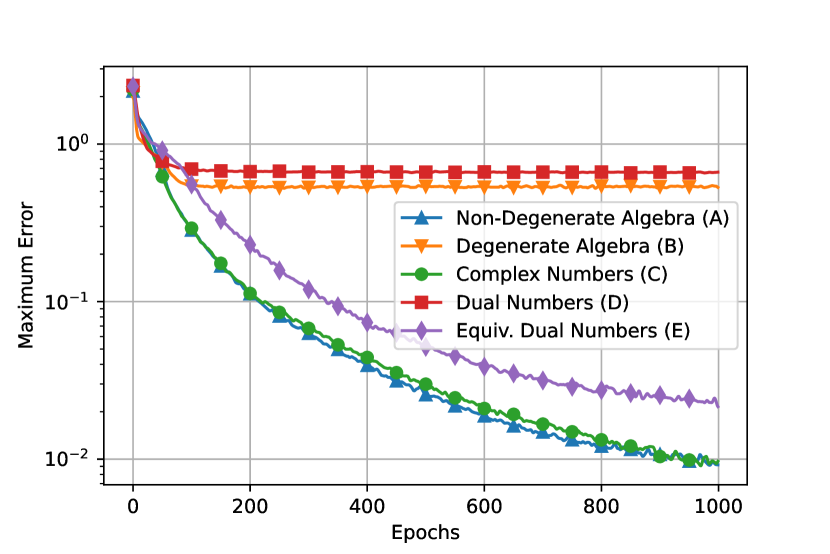
Figure 1: Maximum error by the number of epochs during the training phase of V-MLP networks with real-valued output weights defined on two-dimensional algebras.

In order to validate Theorem 2, we implemented V-MLP networks using the five algebras shown in Table 1. The networks have real-valued output weights and 128 hidden neurons with the split ReLU activation function. They have been trained using a dataset consisting of 1024 samples taken uniformly from $K$. Furthermore, the five V-MLP networks have been trained by minimizing the mean-squared error (MSE) using the Adam optimizer for 1000 epochs. Figure 1 shows the maximum error produced by the V-MLP networks by the number of epochs during the training phase.

Note from Figure 1 that the maximum error decreased consistently for the networks that were based on non-degenerate algebras, namely the networks defined on the algebras $\mathbb{A}$, $\mathbb{C}$ (complex numbers), and $\mathbb{E}$ (the algebra equivalent to dual numbers). In contrast, the maximum error produced by the V-MLP networks based on dual-numbers $\mathbb{D}$ and the degenerate algebra $\mathbb{B}$ stagnated at the values 0.67 and 0.51, respectively. This numerical example confirms the approximation capability of V-MLP networks defined on non-degenerate algebras. It also reveals that Theorem 2 may fail for a V-MLP network defined on a degenerate algebra.

a) Surfaces of the components of the vector-valued function $f_{\mathbb{V}}$.

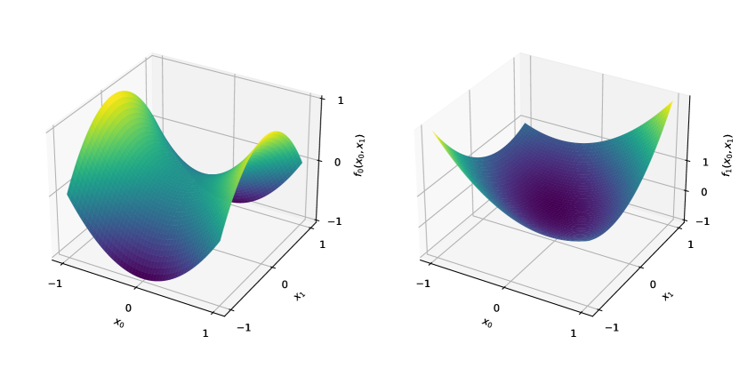
b) Surfaces of the components of the V-MLP network defined on the algebra $\mathbb{B}$.

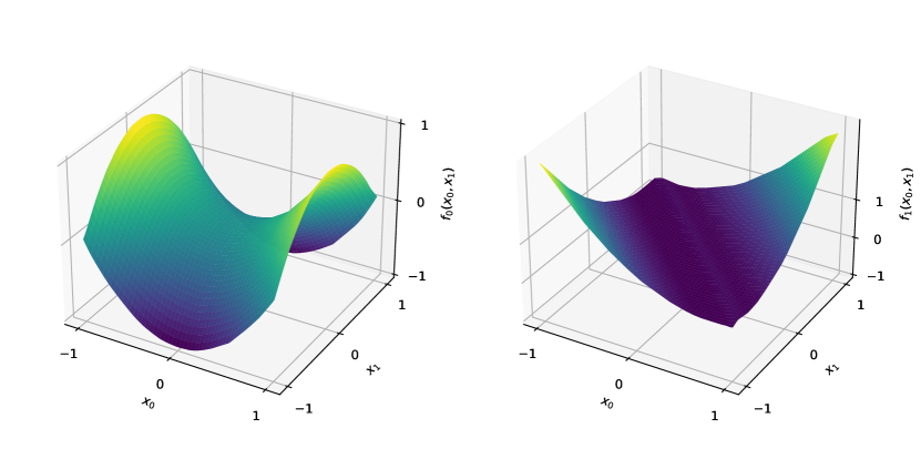
Figure 2: Surfaces of the components of the function $f_{\mathbb{V}}$ given by (35) and the V-MLP networks with real-valued output weights defined on a two-dimensional degenerate algebra.

a) Surfaces of the components of the V-MLP network defined on dual numbers $\mathbb{D}$.

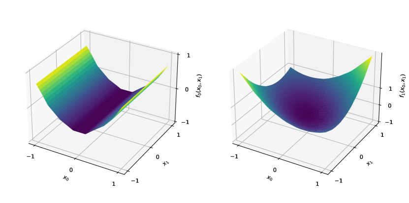
b) Surfaces of the components of the V-MLP network defined on the algebra $\mathbb{E}$.

Figure 3: Surfaces of the V-MLP networks with real-valued output weights defined on the two-dimensional algebras $\mathbb{D}$ (dual numbers) and $\mathbb{E}$ (equivalent to dual numbers).

To better illustrate the approximation capability of the V-MLPs, Figures 2 and 3 display the surfaces associated with the components of $f_{\mathbb{V}}$ and the trained networks defined on the algebras $\mathbb{B}$, $\mathbb{D}$, and $\mathbb{E}$. Note that the V-MLP networks based on the algebra $\mathbb{E}$ visually coincide with the surfaces of $f_{\mathbb{V}}$, despite producing the largest maximum error among the networks defined on non-degenerate algebras. However, the V-MLP networks based on degenerate algebras fail to approximate $f_{\mathbb{V}}$ precisely on the component whose bilinear form is degenerate. Accordingly, in the proof of Theorem 2 included in the appendix, we utilize the non-degeneracy of the bilinear form to determine the weights in the hidden layer of the V-MLP network. Conversely, the network may fail to approximate a component of the continuous function $f_{\mathbb{V}}$ if the corresponding bilinear form is degenerate.

Figure 4: Maximum error by the number of epochs during the training phase of V-MLP networks with vector-valued output weights defined on non-degenerate two-dimensional algebras.

Figure 5: Surfaces of the components of the V-MLP network, with vector-valued output weights, defined on the two-dimensional non-degenerate algebra $\mathbb{A}$.

Finally, to illustrate the second part of Theorem 2, we approximated $f_{\mathbb{V}}$ using V-MLP networks with vector-valued output weights on non-degenerate algebras. We used the same network architecture (128 hidden neurons with split ReLU activation function) and training methodology (we minimized the MSE using the Adam method for 1000 epochs). Figure 4 shows the maximum error by the number of epochs produced by the V-MLP network defined on the non-degenerate algebra $\mathbb{A}$, $\mathbb{C}$, and $\mathbb{E}$. Notice that the maximum error produced by the MLP networks based on the non-degenerate hypercomplex algebras $\mathbb{C}$ and $\mathbb{E}$ decreased consistently. However, the maximum error produced by the network based on the non-degenerate algebra $\mathbb{A}$ (which is not a hypercomplex algebra) stagnated at 1.88. Figure 5 shows the surface of the components of the V-MLP defined on the algebra $\mathbb{A}$. As the bilinear forms associated with components of the product coincide in the algebra $\mathbb{A}$, the surfaces of the two components also coincide.

In conclusion, this second numerical example confirms the approximation capability of MLP networks with hypercomplex-valued output weights defined on non-degenerate algebra. Furthermore, it provides an example of a V-MLP network with vector-valued output weights defined on an algebra without identity that is not able to approximate a given function.

4.2 Numerical Example with Four-Dimensional Algebras

In analogy to the numerical examples given in the previous section, this section illustrates Theorem 2 using the four-dimensional algebras shown in Table 2. Precisely, let $\mathcal{E}=\{\boldsymbol{e}_{0},\boldsymbol{e}_{1},\boldsymbol{e}_{2},\boldsymbol{e}_{3}\}$ be a basis for a four-dimensional algebra $\mathbb{V}$ and consider the vector-valued function $f_{\mathbb{V}}:\mathbb{V}\to\mathbb{V}$ defined by

$$f_{\mathbb{V}}(x)=(x_{0}^{2}+x_{1}x_{2}+x_{3}^{2})\boldsymbol{e}_{0}+(x_{1}^{2}+x_{2}x_{3}+x_{0}^{2})\boldsymbol{e}_{1}+(x_{2}^{2}+x_{3}x_{0}+x_{1}^{2})\boldsymbol{e}_{2}+(x_{3}^{2}+x_{0}x_{1}+x_{2}^{2})\boldsymbol{e}_{3},$$ (37)

for all $x\in K$, where

$$K=\{x=x_{0}\boldsymbol{e}_{0}+x_{1}\boldsymbol{e}_{1}+x_{2}\boldsymbol{e}_{2}+x_{3}\boldsymbol{e}_{3}:x_{0},x_{1},x_{2},x_{3}\in[-1,1]\}\subset\mathbb{V},$$ (38)

is a compact set. Like the function considered previously, the components of $f_{\mathbb{V}}$ given by (37) are quadratic forms on the components $x_{0},x_{1},x_{2}$ and $x_{3}$ of $x$. Therefore, $f_{\mathbb{V}}$ is a continuous but non-linear vector-valued function.

Using the four-dimensional algebras listed in Table 2, we implemented V-MLP networks with 128 hidden neurons with the split ReLU activation function. All the networks have been trained by minimizing the mean-squared error over a dataset with 1024 samples taken uniformly from $K$ and using the Adam optimizer for 1000 epochs. Figures 6 and 7 show the maximum error by the number of epochs for networks with real-valued and vector-valued output weights, respectively.

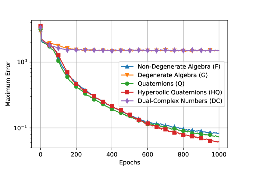
Figure 6: Maximum error by the number of epochs during the training phase of V-MLP networks with real-valued output weights defined on four-dimensional algebras.

Note from Figure 6 that the maximum error consistently decreased for the V-MLP networks with real-valued output weights that were defined on non-degenerate algebras such as the algebra $\mathbb{F}$, the quaternions $\mathbb{Q}$, and the hyperbolic quaternions $\mathbb{HQ}$. In contrast, the maximum error produced by the networks defined on the degenerate algebras $\mathbb{G}$ and $\mathbb{DC}$ (dual-complex numbers) remained stagnant at 1.46 and 1.47, respectively.

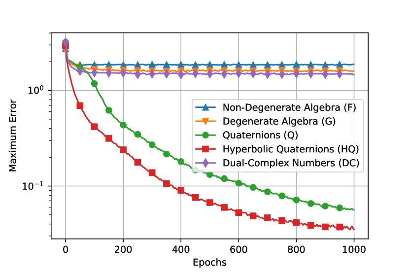
Figure 7: Maximum error by the number of epochs during the training phase of V-MLP networks with vector-valued output weights defined on four-dimensional algebras.

When vector-valued output weights were considered instead of real-valued ones, the maximum error consistently decreased for the MLP networks defined on non-degenerate hypercomplex algebras such as $\mathbb{Q}$ and $\mathbb{HQ}$ (see Figure 7). For the degenerate algebras $\mathbb{G}$ and $\mathbb{DC}$, the maximum error remained stagnant at 1.57 and 1.47, respectively. Moreover, notice that the maximum error remained stagnant at 1.88 for the V-MLP with vector-valued output weights defined on the non-degenerate algebra $\mathbb{F}$, which is not a hypercomplex algebra.

In conclusion, the numerical examples provided in this subsection illustrate the following:

• V-MLP networks with real-valued output weights defined on non-degenerate algebras exhibit approximation capability.

• We can not ensure the approximation capability for a V-MLP with real-valued output weights defined on degenerate algebras. Indeed, the networks defined on the degenerate algebra $\mathbb{G}$ and dual-complex numbers $\mathbb{DC}$ failed to approximate the continuous vector-valued function $f_{\mathbb{V}}$ defined by (37) on the compact set $K\subset\mathbb{V}$.

• Hypercomplex-valued MLP networks with hypercomplex-valued output weights also exhibit the approximation capability on non-degenerate algebras.

• V-MLP networks with vector-valued output weights may not approximate a vector-valued function if the algebra is not hypercomplex. In fact, the V-MLP networks defined on the non-degenerate algebra $\mathbb{F}$ failed to approximate the continuous function $f_{\mathbb{V}}:\mathbb{V}\to\mathbb{V}$ given by (37) on the compact set $K\subset\mathbb{V}$.

5 Concluding Remarks

The universal approximation theorem states that a single hidden layer multi-layer perceptron (MLP) network can accurately approximate continuous functions with arbitrary precision. This important theoretical result was first proven for real-valued networks in the late 1980s and early 1990s by many researchers under different hypotheses on the activation function [12, 15, 20, 27, 35]. In the subsequent years, the universal approximation theorem was also demonstrated for neural networks based on well-known hypercomplex algebras, such as complex [3], quaternions [2], and Clifford algebras [7]. However, each of these results was derived independently, leading to a lack of generality in the approximation capability of hypercomplex-valued networks. In this work, we investigate some of the existing universal approximation theorems and link the approximation capability of hypercomplex-valued networks using the broad class of vector-valued neural networks.

Vector-valued neural networks are similar to real-valued models, but they utilize elements of an algebra $\mathbb{V}$ for weights, bias, inputs, and outputs [44]. An algebra $\mathbb{V}$ is a finite-dimensional vector space with a bilinear operation called multiplication or product (see Definition 1). An algebra is considered hypercomplex if the multiplication has a two-sided identity (see Definition 3). The broad class of V-nets includes complex, quaternion, tessarine, and Clifford-valued models [1, 3, 7, 8, 9, 19] and many other hypercomplex-valued neural networks, for which their approximation capability was previously unknown [17, 36, 50, 43, 47].

Using the approximation capability of real-valued MLP networks, we showed that a V-MLP network with a split-activation function and real-valued output weights can approximate a continuous vector-valued function to any given precision on a compact, provided the algebra is non-degenerate. We also demonstrated the approximation capability of hypercomplex-valued MLP networks with hypercomplex output weights. These results are summarized in Theorem 2, the primary contribution of this paper and whose proof can be found in the appendix.

Concluding, the universal approximation theorem provided in this paper serves multiple purposes. Firstly, it consolidates the results regarding the universal approximation capability of many well-known algebras, eliminating the need to prove this property for each algebra individually. The class of non-degenerate hypercomplex algebras, including the complex and hyperbolic numbers, quaternions, tessarines, and Clifford algebras, are covered in this result. Furthermore, the universal approximation property is now recognized to hold for MLP networks on many other algebras including the Klein group and the octonions [25, 36]. Lastly, Theorem 2 should promote the use of vector- and hypercomplex-valued networks, which are known to perform well in problems involving multidimensional signals, such as images, video, and 3D movement [34, 47]. The universal approximation property strengthens these models’ applications, making them better suited than real-valued models for a wider variety of applications.

Appendix A Proof of Theorem 2

As pointed out previously in Section 4, our proof of Theorem 2 is based on the results by Arena et al. [2]. Accordingly, let us first extend Lemma 3.1 of [2] to finite-dimensional non-degenerate algebras.

Lemma 1 (Representation of Linear Functionals on Non-degenerate Algebras).

Let $\mathbb{V}$ be a finite-dimensional non-degenerate algebra over $\mathbb{R}$ and $\pi_{i}:\mathbb{V}\to\mathbb{R}$ denote a component projection given by (4) for $i\in\{0,1,\ldots,n-1\}$. Given a linear functional $\mathcal{L}:\mathbb{R}^{nN}\to\mathbb{R}$, there exist $y_{1},\ldots,y_{N}\in\mathbb{V}$ such that

$$(\mathcal{L}\circ\varphi)(\boldsymbol{x})=\pi_{i}\left(\sum_{i=1}^{N}y_{j}x_{j}\right),\quad\forall\boldsymbol{x}=(x_{1},\ldots,x_{N})\in\mathbb{V}^{N},$$ (39)

where $\varphi:\mathbb{V}^{N}\to\mathbb{R}^{nN}$ is obtained by applying the isomorphism $\varphi:\mathbb{V}\to\mathbb{R}^{n}$ given by (2) component-wise.

Remark 4.

Because $\mathcal{L}:\mathbb{R}^{nN}\to\mathbb{R}$ and $\varphi:\mathbb{V}^{N}\to\mathbb{R}^{nN}$ are both linear, their composition $\mathcal{L}\circ\varphi:\mathbb{V}^{N}\to\mathbb{R}$ is also a linear functional.

Proof.

Let $L(\mathbb{R}^{nN},\mathbb{R})$ denote the set of all linear functions from $\mathbb{R}^{nN}$ to $\mathbb{R}$, that is,

$$L(\mathbb{R}^{nN},\mathbb{R})=\{\mathcal{L}:\mathbb{R}^{nN}\to\mathbb{R}:\mathcal{L}\;\text{is a linear functional}\}.$$ (40)

Note that

$$\dim\big{(}L(\mathbb{R}^{nN},\mathbb{R})\big{)}=\dim(\mathbb{R}^{nN})\dim(\mathbb{R})=nN.$$ (41)

Thus, using the isomorphism $\varphi:\mathbb{V}^{N}\to\mathbb{R}^{nN}$, we conclude that $\mathbb{V}^{N}$ and $L(\mathbb{R}^{nN},\mathbb{R})$ have the same dimension.

Let $T:\mathbb{V}^{N}\to L(\mathbb{R}^{nN},\mathbb{R})$ be the mapping defined by the following equation for all $\boldsymbol{y}=(y_{1},\ldots,y_{N})\in\mathbb{V}^{N}$:

$$T(\boldsymbol{y})\big{(}\varphi(\boldsymbol{x})\big{)}=\pi_{i}\left(\sum_{j=1}^{N}y_{j}x_{j}\right),\quad\forall\boldsymbol{x}=(x_{1},\ldots,x_{N})\in\mathbb{V}^{N}.$$ (42)

In other words, $T(\boldsymbol{y})=\mathcal{L}$, where $\mathcal{L}:\mathbb{R}^{nN}\to\mathbb{R}$ is the linear functional given by (39). We will show that $T$ is a linear one-to-one mapping.

The linearity of $T$ is a straightforward consequence of the linearity of the component projection $\pi_{i}$. Let us now show that $T$ is an injective mapping or, equivalently, that $\ker(T)=\{\boldsymbol{0}\}\subset\mathbb{V}^{N}$.

From (10), the following identities hold true:

$$T(\boldsymbol{y})\big{(}\varphi(\boldsymbol{x})\big{)}=\pi_{i}\left(\sum_{j=1}^{N}y_{j}x_{j}\right)=\sum_{j=1}^{N}\pi_{i}(y_{j}x_{j})=\sum_{j=1}^{N}\mathcal{B}_{i}(y_{j},x_{j}).$$ (43)

Because the algebra is non-degenerate, by hypothesis, the bilinear form $\mathcal{B}_{i}:\mathbb{V}\times\mathbb{V}\to\mathbb{R}$ is non-degenerate. Thus, we have

$$T(\boldsymbol{y})\big{(}\varphi(\boldsymbol{x})\big{)}=\sum_{j=1}^{N}\mathcal{B}_{i}(y_{j},x_{j})=0_{\mathbb{R}},\quad\forall\boldsymbol{x}=(x_{1},\ldots,x_{N})\in\mathbb{V}^{N},$$ (44)

if and only if $y_{j}=0_{\mathbb{V}}$ for all $j=1,\ldots,N$. Hence, we have $\ker(T)=\{\boldsymbol{0}\}$.

Finally, since $T:\mathbb{V}^{N}\to L(\mathbb{R}^{nN},\mathbb{R})$ is a linear injective mapping between spaces with the same dimension, $T$ is a one-to-one linear mapping.

Concluding, given a linear functional $\mathcal{L}:\mathbb{V}^{N}\to\mathbb{R}$, there exists $\boldsymbol{y}=(y_{1},\ldots,y_{N})\in\mathbb{V}^{N}$ such that $T(\boldsymbol{y})=\mathcal{L}$; namely $\boldsymbol{y}=T^{-1}(\mathcal{L})$. Equivalently, there exist $y_{1},\ldots,y_{N}\in\mathbb{V}^{N}$ such that (39) holds true. ∎

Before proceeding to the proof of Theorem (2), we would like to emphasize that Lemma 1 holds for non-degenerate algebras. The following example illustrates that Lemma 1 may fail for degenerate algebra. Precisely, the following example shows that we cannot represent a given linear function as the component projection of a weighted sum in the hypercomplex algebra of dual numbers.

Example 1.

Let $\mathbb{D}$ denote the hypercomplex algebra of dual numbers, which is an example of a degenerate algebra with respect to the canonical basis $\tau=\{1,\boldsymbol{i}\}$, where $\boldsymbol{i}^{2}=1$. A linear functional $\mathcal{L}:\mathbb{R}^{4}\to\mathbb{R}$ is given by $\mathcal{L}(t_{1},t_{2},t_{3},t_{4})=at_{1}+bt_{2}+ct_{3}+dt_{4}$, for some $a,b,c,d\in\mathbb{R}$. Thus, using the isomorphism $\varphi:\mathbb{D}^{2}\to\mathbb{R}^{4}$, we obtain

$$(\mathcal{L}\circ\varphi)(\boldsymbol{x})=ax_{1,0}+bx_{1,1}+cx_{2,0}+dx_{2,1},\quad\forall\boldsymbol{x}=(x_{1},x_{2})\in\mathbb{D}^{2},$$ (45)

where $x_{1}=x_{1,0}+x_{1,1}\boldsymbol{i}\in\mathbb{D}$ and $x_{2}=x_{2,0}+x_{2,1}\boldsymbol{i}\in\mathbb{D}$. Because $\boldsymbol{i}^{2}=0$, the multiplication of $y=y_{0}+y_{1}\boldsymbol{i}\in\mathbb{D}$ and $x=x_{0}+x_{1}\boldsymbol{i}\in\mathbb{D}$ is $yx=(y_{0}x_{0})+(y_{0}x_{1}+y_{1}x_{0})\boldsymbol{i}$. Moreover, we have

$$\pi_{0}(y_{1}x_{1}+y_{2}x_{2})=y_{1,0}x_{1,0}+y_{2,0}x_{2,0},$$ (46)

where $\pi_{0}:\mathbb{D}\to\mathbb{R}$ denotes the projection into the real part of a dual number, that is, $\pi_{0}(x)=x_{0}$ for all $x=x_{0}+x_{1}\boldsymbol{i}$. Hence, there exist $y_{1}=y_{1,0}+y_{1,1}\boldsymbol{i}\in\mathbb{D}$ and $y_{2}=y_{2,0}+y_{2,1}\boldsymbol{i}\in\mathbb{D}$ such that

$$(\mathcal{L}\circ\varphi)(\boldsymbol{x})=\pi_{0}(y_{1}x_{1}+y_{2}x_{2}),$$ (47)

if, and only if, $b=d=0$. Therefore, there do not exist $y_{1},y_{2}\in\mathbb{D}$ such that (47) holds true for an arbitrary linear functional $\mathcal{L}:\mathbb{R}^{4}\to\mathbb{R}$.

Proof of Theorem 2.

First of all, recall that $\mathcal{H}_{\mathbb{V}}$ is dense in $C(K)$ if, and only if, given a continuous vector-valued function $f_{\mathbb{V}}:K\subset\mathbb{V}^{N}\to\mathbb{V}$ and $\varepsilon>0$, there exists a V-MLP network $\mathcal{N}_{\mathbb{V}}:\mathbb{V}^{N}\to\mathbb{V}$ given by (32) with $w_{ij}\in\mathbb{V}$, $\theta_{i}\in\mathbb{V}$, and $\alpha_{i}\in\mathbb{R}$, for all $i=1,\ldots,M$ and $j=1,\ldots,N$ such that

$$|\mathcal{N}_{\mathbb{V}}(\boldsymbol{x})-f_{\mathbb{V}}(\boldsymbol{x})|\leq\varepsilon,\quad\forall\boldsymbol{x}\in K.$$ (48)

In the following, we use the approximation property of real-valued MLP networks to construct such a V-MLP network.

Let $f_{\mathbb{V}}:\mathbb{V}^{N}\to\mathbb{V}$ be a given continuous vector-valued function and consider $\varepsilon>0$. The vector-valued function $f_{\mathbb{V}}$ can be written as follows

$$f_{\mathbb{V}}(\boldsymbol{x})=\sum_{k=0}^{n-1}f_{k}(\boldsymbol{x})\boldsymbol{e}_{k},\quad\forall\boldsymbol{x}=(x_{1},\ldots,x_{N})\in K\subset\mathbb{V}^{N},$$ (49)

where $f_{k}:K\to\mathbb{R}$ denotes the $k$th componet of $f_{\mathbb{V}}$, for all $k=0,\ldots,n-1$. Using the isomorphism $\varphi:\mathbb{V}\to\mathbb{R}^{n}$ given by (2) and the hypothesis that the activation function $\psi_{\mathbb{R}}:\mathbb{R}\to\mathbb{R}$ yields approximation capability to real-valued MLP networks, there exist real-valued MLP networks $\mathcal{N}_{k}:\mathbb{R}^{nN}\to\mathbb{R}$ such that

$$|\mathcal{N}_{k}\big{(}\varphi(\boldsymbol{x})\big{)}-f_{k}(\boldsymbol{x})|\leq\frac{\varepsilon}{2\sqrt{n}},$$ (50)

for all $\boldsymbol{x}\in K$ and $k=0,\ldots,n-1$. Equivalently, from Remark 1, there exist $M_{k}\in\mathbb{N}$, $\alpha_{ik}\in\mathbb{R}$, $\theta_{ik}^{(\mathbb{R})}\in\mathbb{R}$, and linear functionals $\mathcal{L}_{ik}:\mathbb{R}^{nN}\to\mathbb{R}$ such that

$$\left|\sum_{i=1}^{M_{k}}\alpha_{ij}\psi_{\mathbb{R}}\left(\mathcal{L}_{ik}\big{(}\varphi(\boldsymbol{x})\big{)}-\theta_{ik}^{(\mathbb{R})}\right)-f_{k}(\boldsymbol{x})\right|\leq\frac{\varepsilon}{2\sqrt{n}},$$ (51)

for all $\boldsymbol{x}\in K$ and $k=0,\ldots,n-1$. By hypothesis, the algebra $\mathbb{V}$ is non-degenerate. From Lemma 1, there exist parameters $w_{ijk}\in\mathbb{V}$ such that

$$\left|\sum_{i=1}^{M_{k}}\alpha_{ij}\psi_{\mathbb{R}}\left(\pi_{k}\left(\sum_{j=1}^{N}w_{ijk}x_{j}\right)-\theta_{ik}^{(\mathbb{R})}\right)-f_{k}(\boldsymbol{x})\right|\leq\frac{\varepsilon}{2\sqrt{n}},$$ (52)

We define the V-MLP network by means of the equation for all $\boldsymbol{x}=(x_{1},\ldots,x_{N})\in\mathbb{V}^{N}$

$$\mathcal{N}_{\mathbb{V}}(\boldsymbol{x})=\sum_{k=0}^{n-1}\sum_{i=1}^{M_{k}}\alpha_{ik}\psi_{\mathbb{V}}\left(\sum_{j=1}^{N}w_{ijk}x_{j}+\theta_{ik}\right),$$ (53)

where the bias terms $\theta_{ik}\equiv\theta_{ik}(\lambda)\in\mathbb{V}$ are defined as follows using a parameter $\lambda\in\mathbb{R}$:

$$\theta_{ik}=\theta_{ik}^{(\mathbb{R})}\boldsymbol{e}_{k}+\sum_{\ell\neq k}^{n-1}\lambda\boldsymbol{e}_{\ell}.$$ (54)

Note that (53) is equivalent to (32) if we combine the two sums “$\sum_{k=0}^{n-1}$” and “$\sum_{i=1}^{M_{k}}$” into a single sum “$\sum_{i=1}^{M}$”, with $M=M_{0}+\ldots+M_{n-1}$, and redefine the indexes accordingly. Also, note that the following identity holds for all $\ell=0,\ldots,n-1$:

$$\pi_{\ell}(\theta_{ik})=\begin{cases}\theta_{ik}^{(\mathbb{R})},&\ell=k,\\ \lambda,&\text{otherwise}.\end{cases}$$ (55)

We shall conclude the proof by showing that

$$\left|\mathcal{N}_{\mathbb{V}}(\boldsymbol{x})-f_{\mathbb{V}}(\boldsymbol{x})\right|\leq\varepsilon,\quad\forall\boldsymbol{x}\in K.$$ (56)

Before, however, let us rewrite $\mathcal{N}_{\mathbb{V}}$ using the real-valued MLP networks $\mathcal{N}_{k}:\mathbb{R}^{nN}\to\mathbb{R}$, for $k=0,\ldots,n-1$, which approximate the components of $f_{\mathbb{V}}$. Accordingly, from (5), recalling that $\psi_{\mathbb{V}}:\mathbb{V}\to\mathbb{V}$ is a split activation function derived from $\psi_{\mathbb{R}}:\mathbb{R}\to\mathbb{R}$, and using (55), we have

$$\mathcal{N}_{\mathbb{V}}(\boldsymbol{x}) =\sum_{k=0}^{n-1}\sum_{i=1}^{M_{k}}\alpha_{ik}\left[\sum_{\ell=0}^{n-1}(\pi_{\ell}\circ\psi_{\mathbb{V}})\left(\sum_{j=1}^{N}w_{ijk}x_{j}+\theta_{ik}\right)\boldsymbol{e}_{\ell}\right]$$ (57)

$$=\sum_{k=0}^{n-1}\sum_{i=1}^{M_{k}}\alpha_{ik}\left[\sum_{\ell=0}^{n-1}(\psi_{\mathbb{R}}\circ\pi_{\ell})\left(\sum_{j=1}^{N}w_{ijk}x_{j}+\theta_{ik}\right)\boldsymbol{e}_{\ell}\right]$$ (58)

$$=\sum_{k=0}^{n-1}\sum_{i=1}^{M_{k}}\alpha_{ik}\left[\psi_{\mathbb{R}}\left(\pi_{k}\left(\sum_{j=1}^{N}w_{ijk}x_{j}\right)+\theta_{ik}^{(\mathbb{R})}\right)\boldsymbol{e}_{k}\right.$$ (59)

$$\qquad+\left.\sum_{\ell\neq k}^{n-1}\psi_{\mathbb{R}}\left(\pi_{\ell}\left(\sum_{j=1}^{N}w_{ijk}x_{j}\right)+\lambda\right)\boldsymbol{e}_{\ell}\right]$$

$$=\sum_{k=0}^{n-1}(\mathcal{N}_{k}\circ\varphi)(\boldsymbol{x})\boldsymbol{e}_{k}+\mathcal{R}(\boldsymbol{x},\lambda),$$ (60)

where

$$(\mathcal{N}_{k}\circ\varphi)(\boldsymbol{x})=\sum_{i=1}^{M_{k}}\alpha_{ik}\psi_{\mathbb{R}}\left(\mathcal{L}_{ik}\big{(}\varphi(\boldsymbol{x})\big{)}+\theta_{ik}^{(\mathbb{R})}\right),$$ (61)

corresponds to the real-valued MLP network that approximates the component $f_{k}$ of $f_{\mathbb{V}}$ and

$$\mathcal{R}(\boldsymbol{x},\lambda)=\sum_{k=0}^{n-1}\sum_{i=1}^{M_{k}}\alpha_{ik}\sum_{\ell\neq k}^{n-1}\psi_{\mathbb{R}}\left(\pi_{\ell}\left(\sum_{j=1}^{N}w_{ijk}x_{j}\right)+\lambda\right)\boldsymbol{e}_{\ell}\in\mathbb{V},$$ (62)

is a remainder term that depends on $\boldsymbol{x}\in\mathbb{V}^{N}$ and $\lambda\in\mathbb{R}$. Being $K\subset\mathbb{V}$ a compact and $\pi_{\ell}:\mathbb{V}\to\mathbb{R}$ is continuous, the set

$$B=\left\{\pi_{\ell}\left(\sum_{j=1}^{N}w_{ijk}x_{j}\right):\boldsymbol{x}\in K\right\}\subset\mathbb{R},$$ (63)

is also bounded by the Weierstrass extreme value theorem. By hypothesis, the activation function $\psi_{\mathbb{R}}$ satisfies $\lim_{t\to-\infty}\psi_{\mathbb{R}}(t)=0$. Thus, the remainder $\mathcal{R}(\boldsymbol{x},\lambda)$ tends to zero as $\lambda$ becomes more and more negative. Formally, there exists $\Lambda\geq 0$ such that

$$|\mathcal{R}(\boldsymbol{x},\lambda)|\leq\frac{\varepsilon}{2},\quad\forall\boldsymbol{x}\in K\;\text{and}\;\lambda\leq-\Lambda.$$ (64)

Concluding, using the triangle inequality, the identity (3), and the inequalities (64) and (50), respectively, we obtain

$$\left|\mathcal{N}_{\mathbb{V}}(\boldsymbol{x})-f_{\mathbb{V}}(\boldsymbol{x})\right| =\left|\sum_{k=0}^{n-1}(\mathcal{N}_{k}\circ\varphi)(\boldsymbol{x})\boldsymbol{e}_{k}+\mathcal{R}(\boldsymbol{x},\lambda)-\sum_{k=0}^{n-1}f_{k}(\boldsymbol{x})\boldsymbol{e}_{k}\right|$$ (65)

$$\leq\left|\sum_{k=0}^{n-1}\left((\mathcal{N}_{k}\circ\varphi)(\boldsymbol{x})-f_{k}(\boldsymbol{x})\right)\boldsymbol{e}_{k}\right|+\left|\mathcal{R}(\boldsymbol{x},\lambda)\right|$$ (66)

$$\leq\sqrt{(n-1)\frac{\varepsilon^{2}}{4(n-1)}}+\frac{\varepsilon}{2}=\varepsilon,$$ (67)

for all $\boldsymbol{x}\in K$ and $\lambda\leq-\Lambda$.

Finally, let us prove the second part of the theorem. Because $\mathcal{H}_{\mathbb{V}}$ is dense in the set $\mathcal{C}(K)$ of all continuous functions from $K\subseteq\mathbb{V}^{N}$ to $\mathbb{R}$, given $f_{\mathbb{V}}:\mathbb{V}^{N}\to\mathbb{V}$ and $\varepsilon>0$, there exists a V-MLP $\mathcal{N}_{\mathbb{V}}:\mathbb{V}^{N}\to\mathbb{V}$ given by (32) with $M\in\mathbb{N}$, $\alpha_{i}^{(\mathbb{R})}\in\mathbb{R}$, $w_{ij}\in\mathbb{V}$ and $\theta_{i}\in\mathbb{V}$, for all $i=1,\ldots,M$ and $j=1,\ldots,N$, such that $|\mathcal{N}_{\mathbb{V}}(\boldsymbol{x})-f_{\mathbb{V}}(\boldsymbol{x})|\leq\varepsilon$ for all $\boldsymbol{x}\in K$. However, if $\mathbb{V}\equiv\mathbb{H}$ is a hypercomplex algebra, then there exists $\boldsymbol{1}_{\mathbb{H}}$ such that $\boldsymbol{1}_{\mathbb{H}}x=x$ for all $x\in\mathbb{H}$. Thus, defining $\alpha_{i}=\alpha_{i}^{(\mathbb{R})}\boldsymbol{1}_{\mathbb{H}}\in\mathbb{H}$, we conclude that hypercomplex-valued neural network $\mathcal{N}_{\mathbb{H}}:\mathbb{H}^{N}\to\mathbb{H}$ given by (32) satisfies the following identities:

$$\mathcal{N}_{\mathbb{H}}(\boldsymbol{x})=\sum_{i=1}^{M}\alpha_{i}\psi\left(\sum_{j=1}^{N}w_{ij}x_{j}+\theta_{j}\right)=\sum_{i=1}^{M}\alpha_{i}^{(\mathbb{R})}\psi\left(\sum_{j=1}^{N}w_{ij}x_{j}+\theta_{j}\right).$$ (68)

Therefore, it is equivalent to the V-MLP with real-valued output weights that approximate the hypercomplex-valued continuous function $f_{\mathbb{H}}$. ∎

References

- [1] Aizenberg, I. N. Complex-Valued Neural Networks with Multi-Valued Neurons, 1 ed., vol. 353 of Studies in Computational Intelligence. Springer, Berlin Heidelberg, 2011.
- [2] Arena, P., Fortuna, L., Muscato, G., and Xibilia, M. Multilayer perceptrons to approximate quaternion valued functions. Neural Networks 10, 2 (1 1997), 335–342.
- [3] Arena, P., Fortuna, L., Muscato, G., and Xibilia, M. G. Neural networks in multidimensional domains: fundamentals and new trends in modeling and control. Springer London, 1998.
- [4] Baez, J. C. The octonions. Bulletin of the American Mathematical Society 39 (2002), 145–205.
- [5] Brignone, C., Mancini, G., Grassucci, E., Uncini, A., and Comminiello, D. Efficient Sound Event Localization and Detection in the Quaternion Domain. IEEE Transactions on Circuits and Systems II: Express Briefs (2022), 1–5.
- [6] Buchholz, S., and Sommer, G. A hyperbolic multilayer perceptron. In Proceedings of the IEEE-INNS-ENNS International Joint Conference on Neural Networks (IJCNN 2000) (jul 2000), vol. 2, IEEE, pp. 129–133.
- [7] Buchholz, S., and Sommer, G. Clifford Algebra Multilayer Perceptrons. Springer Berlin Heidelberg, Berlin, Heidelberg, 2001, pp. 315–334.
- [8] Buchholz, S., and Sommer, G. On Clifford neurons and Clifford multi-layer perceptrons. Neural Networks 21, 7 (9 2008), 925–935.
- [9] Carniello, R. A. F., Vital, W. L., and Valle, M. E. Universal Approximation Theorem for Tessarine-Valued Neural Networks. Anais do Encontro Nacional de Inteligência Artificial e Computacional (ENIAC) (11 2021), 233–243.
- [10] Catoni, F., Boccaletti, D., Cannata, R., Catoni, V., Nichelatti, E., and Zampetti, P. The Mathematics of Minkowski Space-Time. Birkhäuser Basel, 2008.
- [11] Cerroni, C. From the theory of congeneric surd equations to segre’s bicomplex numbers. Historia Mathematica 44, 3 (2017), 232–251.
- [12] Cybenko, G. Approximation by superpositions of a sigmoidal function. Mathematics of Control, Signals and Systems 1989 2:4 2, 4 (12 1989), 303–314.
- [13] De Castro, F. Z., and Valle, M. E. Continuous-Valued Octonionic Hopfield Neural Network. In Proceedings Series of the Brazilian Society of Computational and Applied Mathematics (São José dos Campos – Brazil, 2 2018), vol. 6, pp. 1–7.
- [14] Ding, T., and Hirose, A. Online Regularization of Complex-Valued Neural Networks for Structure Optimization in Wireless-Communication Channel Prediction. IEEE Access 8 (2020), 143706–143722.
- [15] Funahashi, K.-I. On the approximate realization of continuous mappings by neural networks. Neural networks 2, 3 (1989), 183–192.
- [16] Grassucci, E., Mancini, G., Brignone, C., Uncini, A., and Comminiello, D. Dual quaternion ambisonics array for six-degree-of-freedom acoustic representation. Pattern Recognition Letters 166 (2 2023), 24–30.
- [17] Grassucci, E., Zhang, A., and Comminiello, D. PHNNs: Lightweight Neural Networks via Parameterized Hypercomplex Convolutions. IEEE Transactions on Neural Networks and Learning Systems (10 2022), 1–13.
- [18] Guizzo, E., Weyde, T., Scardapane, S., and Comminiello, D. Learning Speech Emotion Representations in the Quaternion Domain. IEEE/ACM Transactions on Audio, Speech, and Language Processing 31 (2023), 1200–1212.
- [19] Hirose, A. Complex-Valued Neural Networks, 2nd edition ed. Studies in Computational Intelligence. Springer, Heidelberg, Germany, 2012.
- [20] Hornik, K. Approximation capabilities of multilayer feedforward networks. Neural networks 4, 2 (1991), 251–257.
- [21] Hornik, K., Stinchcombe, M., and White, H. Multilayer feedforward networks are universal approximators. Neural Networks 2, 5 (1 1989), 359–366.
- [22] Huang, J.-S., and Yu, J. Klein four-subgroups of lie algebra automorphisms. Pacific Journal of Mathematics 262, 2 (2013), 397–420.
- [23] Iturrino Garcia, C. A., Bindi, M., Corti, F., Luchetta, A., Grasso, F., Paolucci, L., Piccirilli, M. C., and Aizenberg, I. Power Quality Analysis Based on Machine Learning Methods for Low-Voltage Electrical Distribution Lines. Energies 16, 9 (4 2023), 3627.
- [24] Kantor, I., and Solodovnikov, A. Hypercomplex numbers: an elementary introduction to algebras, vol. 302. Vol. 302. New York: Springer-Verlag,, 1989.
- [25] Kobayashi, M. Hopfield neural networks using klein four-group. Neurocomputing 387 (2020), 123–128.
- [26] Kuroe, Y., and Iima, H. A model of Hopfield-type octonion neural networks and existing conditions of energy functions. In 2016 International Joint Conference on Neural Networks (IJCNN) (2016), pp. 4426–4430.
- [27] Leshno, M., Lin, V. Y., Pinkus, A., and Schocken, S. Multilayer feedforward networks with a nonpolynomial activation function can approximate any function. Neural networks 6, 6 (1993), 861–867.
- [28] Matsumoto, Y., Natsuaki, R., and Hirose, A. Full-Learning Rotational Quaternion Convolutional Neural Networks and Confluence of Differently Represented Data for PolSAR Land Classification. IEEE Journal of Selected Topics in Applied Earth Observations and Remote Sensing 15 (2022), 2914–2928.
- [29] Navarro-Moreno, J., Fernández-Alcalá, R. M., Jiménez-López, J. D., and Ruiz-Molina, J. C. Tessarine Signal Processing under the T-Properness Condition. Journal of the Franklin Institute (8 2020).
- [30] Navarro-Moreno, J., Fernández-Alcalá, R. M., and Ruiz-Molina, J. C. Proper ARMA Modeling and Forecasting in the Generalized Segre’s Quaternions Domain. Mathematics 2022, Vol. 10, Page 1083 10, 7 (3 2022), 1083.
- [31] Nitta, T., and Buchholz, S. On the decision boundaries of hyperbolic neurons. In 2008 IEEE International Joint Conference on Neural Networks (IEEE World Congress on Computational Intelligence) (2008), pp. 2974–2980.
- [32] Nitta, T., and Kuroe, Y. Hyperbolic gradient operator and hyperbolic back-propagation learning algorithms. IEEE Transactions on Neural Networks and Learning Systems 29, 5 (2018), 1689–1702.
- [33] Ortolani, F., Comminiello, D., Scarpiniti, M., and Uncini, A. On 4-Dimensional Hypercomplex Algebras in Adaptive Signal Processing. Smart Innovation, Systems and Technologies 102 (6 2017), 131–140.
- [34] Parcollet, T., Morchid, M., and Linarès, G. A survey of quaternion neural networks. Artificial Intelligence Review 53, 4 (4 2020), 2957–2982.
- [35] Pinkus, A. Approximation theory of the MLP model in neural networks. Acta Numerica 8 (1 1999), 143–195.
- [36] Popa, C.-A. Octonion-valued neural networks. In International Conference on Artificial Neural Networks (2016), Springer, pp. 435–443.
- [37] RD, S. On the algebras formed by the cayley-dickson process. American Journal of Mathematics 76, 2 (1954), 435–46.
- [38] Saoud, L. S., and Ghorbani, R. Metacognitive Octonion-Valued Neural Networks as They Relate to Time Series Analysis. IEEE Transactions on Neural Networks and Learning Systems 31, 2 (2 2020), 539–548.
- [39] Schafer, R. An Introduction to Nonassociative Algebras. Project Gutenberg, 1961.
- [40] Senna, F. R. d., and Valle, M. E. Tessarine and Quaternion-Valued Deep Neural Networks for Image Classification. Anais do Encontro Nacional de Inteligência Artificial e Computacional (ENIAC) (11 2021), 350–361.
- [41] Shang, F., and Hirose, A. Quaternion Neural-Network-Based PolSAR Land Classification in Poincare-Sphere-Parameter Space. IEEE Transactions on Geoscience and Remote Sensing 52 (2014), 5693–5703.
- [42] Siegel, J. W., and Xu, J. Approximation rates for neural networks with general activation functions. Neural Networks 128 (2020), 313–321.
- [43] Takahashi, K. Comparison of high-dimensional neural networks using hypercomplex numbers in a robot manipulator control. Artificial Life and Robotics 26, 3 (8 2021), 367–377.
- [44] Valle, M. E. Understanding vector-valued neural networks and their relationship with real and hypercomplex-valued neural networks, 2023.
- [45] Vaz, J., and da Rocha, R. An Introduction to Clifford Algebras and Spinors. Oxford University Press, 2016.
- [46] Vieira, G., and Valle, M. E. Acute Lymphoblastic Leukemia Detection Using Hypercomplex-Valued Convolutional Neural Networks. In 2022 International Joint Conference on Neural Networks (IJCNN) (7 2022), IEEE, pp. 1–8.
- [47] Vieira, G., and Valle, M. E. A general framework for hypercomplex-valued extreme learning machines. Journal of Computational Mathematics and Data Science 3 (2022), 100032.
- [48] Vital, W. L., Vieira, G., and Valle, M. E. Extending the Universal Approximation Theorem for a Broad Class of Hypercomplex-Valued Neural Networks. Lecture Notes in Computer Science 13654 LNAI (2022), 646–660.
- [49] Voigtlaender, F. The universal approximation theorem for complex-valued neural networks. Applied and Computational Harmonic Analysis 64 (5 2023), 33–61.
- [50] Wu, J., Xu, L., Wu, F., Kong, Y., Senhadji, L., and Shu, H. Deep octonion networks. Neurocomputing 397 (7 2020), 179–191.