Effective Single Particle Theory for Active System

Abstract

A collection of active self-propelled particles exhibits motility-induced phase separation at a packing density much lower than the corresponding equilibrium counterpart. Unlike the equilibrium counterpart, the steady state in a system of active particles is characterized by the continuous association and dissociation of clusters. In this work we propose an effective single-particle model, in which the effect of neighboring particles is replaced by a time-dependent local density around the particle, having a unique auto-correlation function. Such that the local density around the particles has a memory with a finite correlation time. The correlation time increases with packing density. Further, by using the same local density and its correlation function, we solve the system of many particles and compare the results with numerical simulations. Our proposed analytical theory matches well with the numerical study.

I introduction

Active matter is a class of non-equilibrium systems composed of elements that consume energy from the surroundings and convert it into directed motion [1, 2, 3, 4, 5, 6, 7, 8, 9, 10, 11, 12]. Examples of active matter systems range from the biological realm to synthetically engineered materials and exist on the micro as well as macro scale. Biological microswimmers such as E. coli bacteria [13], groups of animals such as fish schools [14] and bird flocks [15], colloidal suspensions, artificial microswimmers and robots are all examples of active matter systems. Such systems are intrinsically far from equilibrium due to the constant supply of energy used for self-propulsion and thus exhibit novel features and properties that are studied using the frameworks of nonequilibrium statistical physics.

The simplest microscopic model used to understand the characteristics of active matter systems is a collection of active Brownian particles (ABPs) [16, 17, 18, 19, 20, 21, 22], consisting of disk-shaped particles which self-propel with a constant speed and the direction of velocity is continuously re-oriented by random thermal fluctuations. Hence, each particle has a tendency to remember its direction up to a time before it reorients in some other direction. This leads to breaking of time-reversal symmetry in the system, even at the single particle level, which makes such systems very different from other nonequilibrium systems [23, 24, 25, 26, 27].
A collection of active Brownian particles shows some novel properties and interesting collective behavior. One such interesting feature is the motility-induced phase separation (MIPS) which occurs solely due to the competing effect of mutual exclusion and activity. [7, 28, 29, 30, 31, 32, 33, 34, 35, 36] Many experiments and simulations are in strong agreement to understand the mechanism of MIPS. It is found that motility leads to local clustering of particles, and further, such local clustering suppresses the activity and leads to negative diffusivity and clustering of particles.
Different features and properties of a collection of active Brownian particles have been studied extensively using numerical simulations. Many recent studies [37, 38, 39] have focused on developing field-theoretic equation for the local density of particles. Such studies successfully explain the macroscopic properties of the system. However, an effective theoretical understanding of the dynamics of a single particle in the presence of other particles is still lacking. Here, we propose an analytical model for the dynamics of a collection of ABPs with an effective single-particle theory, where the interaction among the particles is accounted by a local density-dependent self-propelled speed. We assume that the self-propulsion speed of the particle depends on the local time-dependent density, unlike the mean density of the system as proposed in earlier studies [7, 40]. In addition to this, to account for the local interaction among the particles, we assume that the local density is a random variable that has a unique auto-correlation function, such that the local density at a point decays exponentially with time. The correlation time monotonically increases by increasing the packing density in the system, and it shows a transition around the same critical density beyond which the system exhibits MIPS. Further, we construct the Langevin’s equations of motion for the particle in our analytical model and solve them using the assumed properties of the local density variable in order to find an expression for the mean squared displacement of the particle. We finally verify our analytical model by comparing it with the results obtained from the numerical simulation of the system, and both analytical and numerical results agree well for the range of system packing densities.

II Model

We first discuss the effective single-particle analytical model, introduced here.

Analytical model- Consider a single particle experiencing a local density $\rho(t)$ around it due to the interaction with all the other particles and its speed depends on the local density. In a collection of active Brownian particles, this local density is a time-dependent random variable, and each particle tends to retain the local density around it for a finite time before it changes. This is taken care by assuming that the density auto-correlation function $C_{\rho}(t)$ exponentially decay with time. Hence, the effect of many-particle interactions can be replaced by having a time-dependent density around a single particle. Further, the density decays exponentially with time with a characteristic time scale, which is a function of packing density $\phi$. In this manner, each particle can be treated as non-interacting, and the system can be solved exactly. All the effect of interaction is taken care of in the time-dependent auto-correlation of local density $C_{\rho}(t)$.

Using the local density dependence of effective speed $v(\rho(t))$ we construct the Langevin [41, 42, 43, 44] equations of motion.

$$\frac{dx}{dt}=v(\rho(t))cos(\theta(t))=v_{0}(1-\lambda\rho(t))cos[\theta(t)]$$ (1)

$$\frac{dy}{dt}=v(\rho(t))sin(\theta(t))=v_{0}(1-\lambda\rho(t))sin[\theta(t)]\\$$ (2)

$$\frac{d\theta}{dt}=\sqrt{2D_{R}}\eta(t)$$ (3)

The local density $\rho(t)$ has following properties $<\rho(t)>=\rho_{0}$ and $<\rho(0)\rho(t)>=\rho^{2}exp(-t/\tau(\phi))$, $\rho^{2}=<\rho(0)\rho(0)>$, where $<..>$ is the ensemble average. $\rho_{0}$ is mean density and $\tau(\phi)$ is the correlation-time, which depends on the packing fraction of the system. We further calculate the mean square displacement of the particle. To obtain the mean squared displacement, we need to solve the above three stochastic differential equations. First, we will solve equation 3 as it is independent of other variables x and y.

$$\theta(t)=\sqrt{2D_{R}}\int_{0}^{t}\eta(t^{\prime})dt^{\prime}$$ (4)

$$<\theta(t)>=\sqrt{2D_{R}}\int_{0}^{t}<\eta(t^{\prime})>dt^{\prime}=0\\$$ (5)

$$<\theta^{2}(t)>=2D_{R}\int_{0}^{t}\int_{0}^{t}<\eta(t_{1})\eta(t_{2})>\,dt_{1}\,dt_{2}=2D_{R}t\\$$ (6)

Since $\theta(t)$ corresponds to the sum of many random variables over time, its value is expected to follow a probability density function that can be deduced from Wick’s theorem [45] and using mean and variance of $\theta$ from equations 5 and 6:

$$P(\theta(t))=\frac{1}{\sqrt{4\pi D_{R}t}}e^{\frac{-\theta^{2}}{4D_{R}t}}$$

Now, solving equations of motion for position, 1 and 2

$$x(t)=\int_{0}^{t}{v_{0}}(1-\lambda\rho(t^{\prime}))cos(\theta(t^{\prime}))dt^{\prime}$$

$$y(t)=\int_{0}^{t}{v_{0}}(1-\lambda\rho(t^{\prime}))sin(\theta(t^{\prime}))dt^{\prime}$$

Calculating the second moments of x and y displacements:

$$<x^{2}(t)>={v_{0}}^{2}\int_{0}^{t}\int_{0}^{t}<cos(\theta_{1})cos(\theta_{2})>\,dt_{1}\,dt_{2}+{v_{0}}^{2}\lambda^{2}\int_{0}^{t}\int_{0}^{t}<cos(\theta_{1})cos(\theta_{2})><\rho(t_{1})\rho(t_{2})>\,dt_{1}\,dt_{2}$$

$$-2{v_{0}}^{2}\lambda\int_{0}^{t}\int_{0}^{t}<\rho(t)><cos(\theta_{1})cos(\theta_{2})>\,dt_{1}\,dt_{2}$$

$$<y^{2}(t)>={v_{0}}^{2}\int_{0}^{t}\int_{0}^{t}<sin\theta_{1})sin(\theta_{2})>\,dt_{1}\,dt_{2}+{v_{0}}^{2}\lambda^{2}\int_{0}^{t}\int_{0}^{t}<sin\theta_{1})sin(\theta_{2})><\rho(t_{1})\rho(t_{2})>\,dt_{1}\,dt_{2}$$

$$-2{v_{0}}^{2}\lambda\int_{0}^{t}\int_{0}^{t}<\rho(t)><sin\theta_{1})sin(\theta_{2})>\,dt_{1}\,dt_{2}$$

simplifying both the terms

$$<x^{2}(t)>={v_{0}}^{2}(1-2\lambda\rho_{0})\int_{0}^{t}\int_{0}^{t}<cos(\theta_{1})cos(\theta_{2})>\,dt_{1}\,dt_{2}+{v_{0}}^{2}\lambda^{2}\int_{0}^{t}\int_{0}^{t}<\rho(t_{1})\rho(t_{2})><cos(\theta_{1})cos(\theta_{2})>\,dt_{1}\,dt_{2}$$

$$<y^{2}(t)>={v_{0}}^{2}(1-2\lambda\rho_{)}\int_{0}^{t}\int_{0}^{t}<sin(\theta_{1})sin(\theta_{2})>\,dt_{1}\,dt_{2}+{v_{0}}^{2}\lambda^{2}\int_{0}^{t}\int_{0}^{t}<\rho(t_{1})\rho(t_{2})><sin(\theta_{1})sin(\theta_{2})>\,dt_{1}\,dt_{2}$$

To evaluate both of these expressions, we will find two useful relations using the probability distribution of $\theta$. $\theta_{0}=<\theta(t)>$ and $\sigma^{2}=<\theta^{2}(t)>-{<\theta(t)>}^{2}$. For an active Brownian particle $<\theta(t)>=0$ and $\sigma^{2}=2D_{R}t$, hence

$$<cos(\alpha\theta)>=e^{-D_{R}t}$$ (7)

$$<sin(\alpha\theta)>=0$$ (8)

Further we will calculate the value of $<cos(\theta_{1})cos(\theta_{2})>$ and $<sin(\theta_{1})sin(\theta_{2})>$

$$<cos(\theta_{1})cos(\theta_{2})>=<cos(\theta_{1})cos(\theta_{2})>_{t_{1}>t_{2}}+<cos(\theta_{1})cos(\theta_{2})>_{t_{2}>t_{1}}$$

$$<cos(\theta_{1})cos(\theta_{2})>_{t_{1}>t_{2}}=\int d\theta_{1}\int d\theta_{2}cos(\theta_{1})cos(\theta_{2})\frac{1}{\sqrt{4\pi D_{R}(t_{1}-t_{2})}}e^{\frac{-{(\theta_{1}-\theta_{2})}^{2}}{4D_{R}(t_{1}-t_{2})}}\frac{1}{\sqrt{4\pi D_{R}t_{2}}}e^{\frac{-{(\theta_{2}-\theta_{0})}^{2}}{4D_{R}t_{2}}}$$

Using the results of eqn LABEL:cos with $\theta_{0}=\theta_{2}$ and $\sigma^{2}=2D_{R}(t_{1}-t_{2})$ first integrating over $d\theta_{1}$ and then with $\theta_{0}=0$ $\sigma^{2}=2D_{R}t_{2}$

$$<cos(\theta_{1})cos(\theta_{2})>_{t_{1}>t_{2}}=\frac{1}{2}e^{-D_{R}(t_{1}-t_{2})}(1+e^{-4D_{R}t_{2}})$$ (9)

similarly

$$<cos(\theta_{1})cos(\theta_{2})>_{t_{2}>t_{1}}=\frac{1}{2}e^{-D_{R}(t_{2}-t_{1})}(1+e^{-4D_{R}t_{1}})$$ (10)

$$<sin(\theta_{1})sin(\theta_{2})>_{t_{1}>t_{2}}=\frac{1}{2}e^{-D_{R}(t_{1}-t_{2})}(1+e^{-4D_{R}t_{2}})$$ (11)

$$<sin(\theta_{1})sin(\theta_{2})>_{t_{2}>t_{1}}=\frac{1}{2}e^{-D_{R}(t_{2}-t_{1})}(1+e^{-4D_{R}t_{1}})$$ (12)

We will exploit these relations to find the second moments of x and y displacements

$$\Delta(t)=<x^{2}(t)>+<y^{2}(t)>$$

$$={v_{0}}^{2}(1-2\lambda\rho_{0})[\int_{0}^{t}\int_{0}^{t}<cos(\theta_{1})cos(\theta_{2})>\,dt_{1}\,dt_{2}+\int_{0}^{t}\int_{0}^{t}<sin(\theta_{1})sin(\theta_{2})>\,dt_{1}\,dt_{2}]$$

$$+{v_{0}}^{2}\lambda^{2}[\int_{0}^{t}\int_{0}^{t}<\rho(t_{1})\rho(t_{2})><cos(\theta_{1})cos(\theta_{2})>\,dt_{1}\,dt_{2}+\int_{0}^{t}\int_{0}^{t}<\rho(t_{1})\rho(t_{2})><sin(\theta_{1})sin(\theta_{2})>\,dt_{1}\,dt_{2}]$$

Using the expression $<\rho(0)\rho(t)>=\rho^{2}exp(-t/\tau(\phi))$

$$\Delta(t)=\frac{2{v_{0}}^{2}}{{D_{R}}^{2}}(1-2\lambda\rho_{0})[D_{R}t-1+e^{-D_{R}t}]+\frac{2{v_{0}}^{2}\lambda^{2}\rho^{2}}{{\beta}^{2}}[\beta t-1+e^{-\beta t}]$$ (13)

Now we further define the effective diffusivity from our effective single particle theory $D_{eff,ef}(\phi)=\lim_{t\rightarrow\infty}\frac{\Delta(t)}{4t}$

$$D_{eff,ef}(\phi)=\frac{{v_{0}}^{2}}{2D_{R}}(1-2\lambda\rho_{0})+\frac{{v_{0}}^{2}\lambda^{2}}{2\beta}\rho^{2}$$ (14)

where $\beta=(D_{R}+\frac{1}{\tau})$, and $\rho_{0}$ and $\rho^{2}$ varies linearly and quadratically with packing density $(\phi)$ of particles in the system.

Now we test the mean square displacement $\Delta(t)$ as found from the effective model and from the full numerical simulation.

Numerical model- We consider a system consisting of $N$ disc-shaped active Brownian particles (ABPs) of radius $a$ in a box of size $L$. The self-propulsion speed of each particle is $v$, and its orientation ${\bf\hat{n}_{i}}$ = $(cos\theta_{i},sin\theta_{i})$ is defined by the angle $\theta_{i}$ that the velocity vector makes with the positive x-axis. The ABPs interact according to a short-ranged and repulsive harmonic potential such that the force $\bm{F_{ij}}$ between particles $i$ and $j$ is given by: $\bm{F_{ij}}=-k(2a-\bm{r_{ij}})\bm{\hat{r}_{ij}}$ if $r_{ij}\leq 2a$ and $\bm{F_{ij}}=0$ if $r_{ij}>2a$.
The Langevin equations of motion of the $i^{th}$ particle are:

$$\partial_{t}{\bf{r}}_{i}=v{\bf\hat{{n}}_{i}}+\mu\sum_{j\neq i}{\bf{F}}_{ij}$$ (15)

$$\partial_{t}\theta_{i}=\sqrt{2D_{R}}\eta_{i}(t)$$ (16)

where $v$ is the self propulsion speed, $\mu$ is the mobility and $\sum_{j\neq i}{\bf{F}}_{ij}$ accounts for the net force experienced by the $i^{th}$ particle due to all other particles. $D_{R}$ is the rotational diffusion constant, and $\eta_{i}(t)$ is white Gaussian noise which has zero mean and is delta correlated $<\eta_{i}(t_{1})\eta_{j}(t_{2})>=\delta_{ij}\delta(t_{1}-t_{2})$. We have performed numerical simulations of the above described interacting active Brownian particle system by implementing the equations (15) and (16). In numerical analysis, we have used a set of different values of packing fractions $\phi=\pi a^{2}N/L^{2}$ and the self-propulsion speed $v_{0}=1.0$. Similar numerical simulations have already been used extensively, such as in [7], in which the dynamics of the system is described by the mean square displacement $\Delta(t,\phi)$ and the late time effective diffusivity of the particle for different packing densities, $D_{eff}(\phi)=\lim_{t\rightarrow\infty}\frac{\Delta(t,\phi)}{4t}$ of the particle for different packing densities. Further the effective self-propulsion speed of the particle is defined as $v(\phi)=\sqrt{(}2D_{R}D_{eff}(\phi))$.

Figure 1: Effective speed $v(\phi)$ vs. mean density $\rho_{0}$. Inset: $D_{eff}$ vs. mean density $\rho_{0}$.

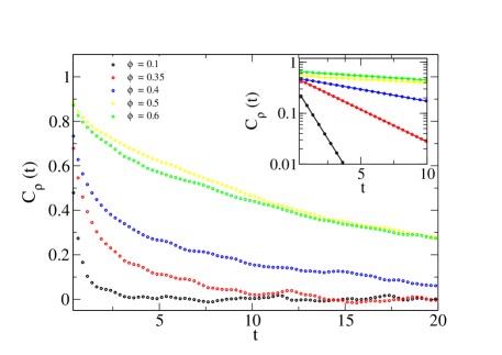
Figure 2: Density auto-correlation $C_{\rho}(t)$ vs. time for different packing fractions $\phi$. Inset: The same plot as main, zoomed for small time and plotted on semi-$\log$-y scale. Lines are exponential fit and data points are from numerical simulation.

Figure 3: The correlation time $\tau$ vs. packing fraction $\phi$.

In Fig. 1 we show the variation of the effective speed $v(\phi)$ and in the inset the $D_{eff}(\phi)$ vs. mean density $\rho_{0}$. The mean density is obtained from the mean of the local density $\rho(t)$ around a particle. The local density $\rho(t)$ around a particle is obtained by simply counting the number of interacting neighbors are in contact and normalizing the number by $6$, assuming the formation of hexagonal close packed structure (HCP) for strong clustering. Then further we obtain the mean of $\rho(t)$, over all the particles and times in the steady state. We also compared the relation between the mean density $<\rho(t)>=\rho_{0}$ with packing density $\phi$ and it varies linearly with packing density (data not shown). The speed of the particle $v(\phi)$ varies approximately linearly with the mean density $\rho_{0}$ as $v(\phi)=v_{0}(1-\lambda\rho_{0})$, where $<\rho>=\rho_{0}$ is a function of packing density $\phi$ as stated previously. The data points in Fig. 1 is obtained from the simulation using the inset plot of effective diffusivity $D_{eff}$, and the line is the linear fit. From the fit we estimate the parameter $\lambda=1.18\pm 0.01$.
Now, we further analyze how the local density around a particle changes in the system. We calculate the auto-correlation function of the local density, defined as $C_{\rho}(t)=<\rho_{i}(0)\rho_{i}(t)>$. Where $<..>$ means average over all the particles and many reference times in the steady state. In Fig.2 we show the plot of $C_{\rho}(t)$ vs. $t$. The $C_{\rho}(t)$, increases by increasing packing density $\phi$. In the inset of Fig.2 we plot $C_{\rho}(t)$ vs. $t$ on semi-log $y-$scale. For all packing densities $C_{\rho}(t)$ decays exponentially with time. The lines in the inset plots show the exponential fits to the numerical data of $C_{\rho}(t)$ for each packing fraction, which are straight lines on semi-log $y-$scale. From each fit we calculate the correlation time $\tau$ for different packing densities $\phi$. Further in Fig. 3 we show the variation of $\tau$ vs. packing density $\phi$. Very clearly, $\tau$ shows a phase transition type characteristics on increasing $\phi$. For small packing densities, $\phi<0.35$ the correlation time $\tau$ is small. As we increase packing density, the $\tau$ increases monotonically with an abrupt change for $\phi$ close to $0.4$. To show the effect of packing density on the local density around the particle and auto-correlation time we show the snapshots of the local density in Fig. 4(a-d) for four packing densities $\phi=0.1,0.3,0.4$ and $0.5$ respectively and at a given time instant. We clearly see the effect of local density on the clustering in the system. For small packing density $\phi<0.35$ Fig. 4(a), clustering is weak, for moderate packing density $\phi\simeq 0.4$, particles start to form clusters and for $\phi>0.4$, we find prominent clustering in the system as shown in Fig. 4(b-c-d) respectively.

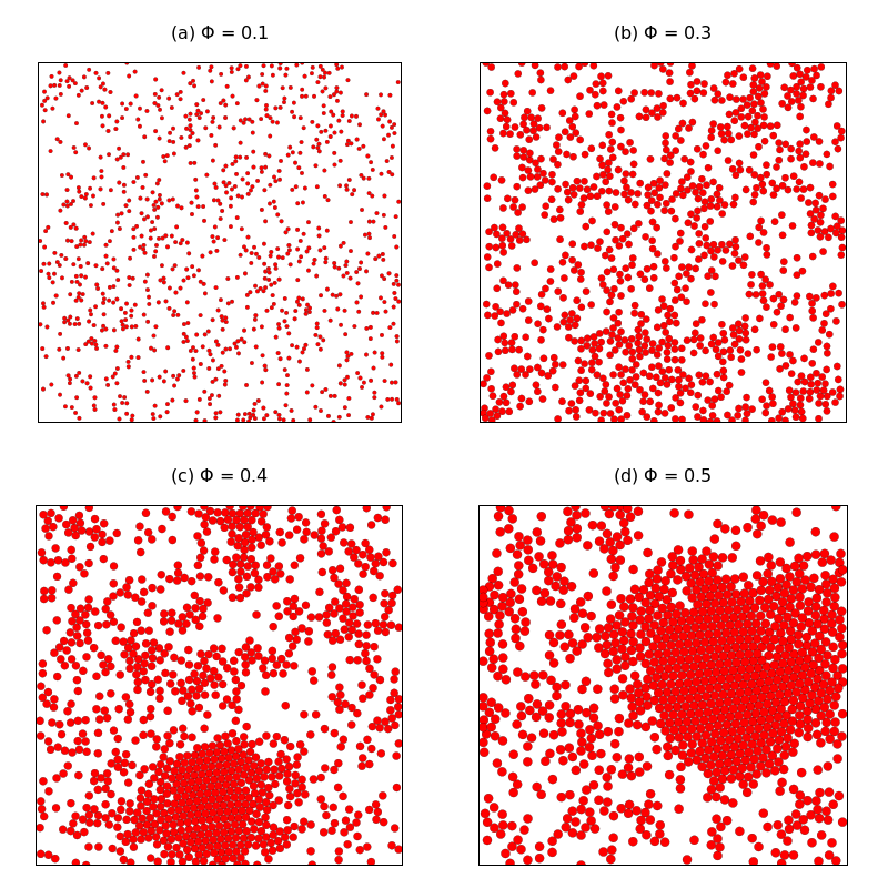
Figure 4: Snapshots of the system of N$=10^{3}$ particles for different packing fractions. For packing fractions below the critical packing fraction $\phi_{c}\approx 0.4$ in $(a)$ and $(b)$, small clusters are formed which form and dissociate continuously. Above the critical packing fraction in $(c)$ and $(d)$, the system phase separates into a single dense cluster.

Fig. 5 shows the plot of $\Delta(t)$ vs. $t$ for four different packing densities $\phi=0.1,0.3,0.4$ and $0.5$. The two solid lines are the expression obtained from the effective single particle theory ($ef$) eqn. 13, mean field ($mf$) model proposed in [7] and dashed line is data from the numerical simulation. We find that the our analytical result matches well with the numerical result for small packing densities $\phi<0.3$. As we increase packing density deviation starts but the effective model is always closer to the numerical data. Finally we compare our model by showing the comparison of effective diffusivities from the analytical models and numerical data $\Delta D_{eff,ef}(\phi)=\frac{D_{eff,ef}(\phi)}{D_{eff}(\phi)}$ and $\Delta D_{eff,mf}(\phi)=\frac{D_{eff,mf}(\phi)}{D_{eff}(\phi)}$ matches very well for the low packing densities and as we go towards higher density deviation starts. In the table 1 we compare the numerical values of effective diffusivities for different packing densities from the three methods (Numerical, effective single particle, mean field).

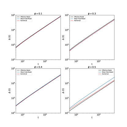
Figure 5: Mean squared displacement of particle for four different packing fractions estimated using the effective single-particle model and mean-field model, compared with the numerical results.

$\phi$	$D_{eff}$	$D_{eff,ef}$	$D_{eff,mf}$	$\Delta D_{eff,ef}$	$\Delta D_{eff,mf}$
0.10	4.14$\pm$0.001	4.29	4.05	0.03$\pm$0.006	0.02$\pm$0.001
0.20	3.27$\pm$0.001	3.51	3.22	0.07$\pm$0.004	0.02$\pm$0.004
0.30	2.46$\pm$0.001	2.74	2.48	0.11$\pm$0.003	0.01$\pm$0.002
0.32	2.27$\pm$0.006	2.54	2.34	0.12$\pm$0.003	0.03$\pm$0.0004
0.40	1.81$\pm$0.002	1.84	1.96	0.02$\pm$0.001	0.08$\pm$0.004
0.50	0.83$\pm$0.004	0.74	1.29	0.11$\pm$0.008	0.55$\pm$0.001
0.60	0.49$\pm$0.006	0.31	0.84	0.37$\pm$0.006	0.70$\pm$0.002

Table 1: Effective diffusivity values estimated using the effective single particle model and mean field model and comparing it with the estimated diffusivity using numerical simulation for different values of packing fraction.

III Discussion

In summary, we have devised a theoretical model that describes the dynamics of an active Brownian particle in the presence of mutual interaction with other particles. In previous studies, the many-particle effect is either studied using microscopic numerical simulation [7, 46, 28, 29, 30, 31, 32, 33, 34, 35, 36] or with the help from effective coarse-grained model for local density [37, 40]. In the present work, we have captured the effect of interaction with all other particles on a single ABP into an effective interacting model. We introduce a local density variable $\rho(t)$ around the particle and set the speed of the particle to vary with the local density it experiences at a point at fixed time. The auto-correlation of the density decay exponentially with time. And the system is characterized by correlation time, which solely depends on the packing density in the system. The correlation time $\tau(\phi)$ increases monotonically with increasing packing density and shows a phase transition type feature as system goes from low density non-clustered phase to large density motility induced phase separating regime. With the help of such time dependence density we developed an effective single particle model and compared the results from analytical theory and numerical simulation. Our effective single particle theory matches well with the numerical results.
Hence through this study we were able to develop an effective single particle model for the collection of interacting self-propelled particle system. The key ingredient of the model is the time dependence of the local density around the particle. The property of which is characterised by a correlation time. Such correlation time can be measured in experiments by simply tracking the density of particles around some tag particles. Once this time is obtained then many particle interacting system can be replaced by our effective single particle model.