Recognition of Unit Segment and Polyline Graphs is $\exists\mathbb{R}$-Complete

Abstract

Given a set of objects $O$ in the plane, the corresponding intersection graph is defined as follows. A vertex is created for each object and an edge joins two vertices whenever the corresponding objects intersect. We study here the case of unit segments and polylines with exactly $k$ bends. In the recognition problem, we are given a graph and want to decide whether the graph can be represented as the intersection graph of certain geometric objects. In previous work it was shown that various recognition problems are $\exists\mathbb{R}$-complete, leaving unit segments and polylines as few remaining natural cases. We show that recognition for both families of objects is $\exists\mathbb{R}$-complete.

Acknowledgements.

This research started at the 19th Gremo Workshop on Open Problems in Binn VS, Switzerland, in June 2022. We thank the organizers for the invitation and for providing a very pleasant and inspiring working atmosphere. Tillmann Miltzow is generously supported by the Netherlands Organisation for Scientific Research (NWO) under project no. VI.Vidi.213.150. Lasse Wulf is generously supported by the Austrian Science Fund (FWF): W1230.

1 Introduction

Many real-life problems can be mathematically described in the language of graphs. For instance, Cellnex Telecom owns more than $2000$ cell towers in Switzerland. We want to assign each tower a frequency such that no two towers that overlap in coverage use the same frequency. This becomes a graph coloring problem. Every cell tower becomes a vertex, overlap indicates an edge and a frequency assignment corresponds to a proper coloring of the vertices, see Figure 1.

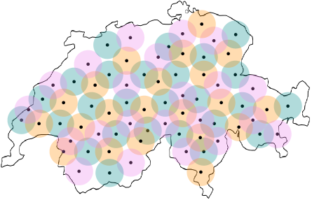
Figure 1: A fictional illustration of mobile coverage of Switzerland using cell towers.

In many contexts, we have additional structure on the graph that may or may not help us to solve the underlying algorithmic problem. For instance, it might be that the graph arises as the intersection graph of unit disks in the plane (each unit disk gives a vertex, and two vertices are adjacent if their corresponding disks overlap). In that case, the coloring problem can be solved more efficiently [10], and there are better approximation algorithms for the clique problem [11]. This motivates a systematic study of geometric intersection graphs. Another motivation is mathematical curiosity. Simple geometric shapes are easily visualized and arguably very natural mathematical objects. Studying the structural properties of intersection graphs gives insight into those geometric shapes and their possible intersection patterns.

It is known for a host of geometric shapes that it is $\exists\mathbb{R}$-complete to recognize their intersection graphs [28, 14, 25, 27]. The class $\exists\mathbb{R}$ consists of all of those problems that are polynomial-time equivalent to deciding whether a polynomial $p\in\mathbb{Z}[X_{1},\ldots,X_{n}]$ has a root. We will introduce $\exists\mathbb{R}$ in more detail below. $\exists\mathbb{R}$-completeness is known for the recognition problems of intersection graphs for segments, disks, unit disks, rays, grounded segments, downward rays, and a few other examples.

In this work, we focus on two geometric objects; unit segments and polylines with exactly $k$ bends. Although we consider both types of geometric objects natural and well studied, to the best of our knowledge the complexity of their recognition problem was left open. We close this gap by showing that both recognition problems are $\exists\mathbb{R}$-complete.

1.1 Definition and Results

We define geometric intersection graphs and the corresponding recognition problem.

Intersection graphs.

Given a finite set of geometric objects $O$, we denote by $G(O)=(V,E)$, the corresponding intersection graph. The set of vertices is the set of objects ($V=O$) and two objects are adjacent ($uv\in E$) if they intersect ($u\cap v\neq\emptyset$). We are interested in intersection graphs that come from different families of geometric objects.

Families of geometric objects.

Examples for a family of geometric objects are segments, disks, unit disks, unit segments, rays, and convex sets, to name a few of the most common ones. In general, given a geometric body $O\subset\mathbb{R}^{2}$ we denote by $O^{\includegraphics[scale={0.15},page=2]{figures/rotation.pdf}}$ the family of all translates of $O$. Similarly, we denote by $O^{\includegraphics[scale={0.15}]{figures/rotation.pdf}}$ the family of all translates and rotations of $O$. For example, the family of all unit segments can be denoted as $u^{\includegraphics[scale={0.15}]{figures/rotation.pdf}}$, where $u$ is a unit segment.

Graph classes.

Classes of geometric objects $\mathcal{O}$ naturally give rise to classes of graphs $C(\mathcal{O})$: Given a family of geometric objects $\mathcal{O}$, we denote by $C(\mathcal{O})$ the class of graphs that can be formed by taking the intersection graph of a finite subset from $\mathcal{O}$.

Recognition.

If we are given a graph, we can ask if this graph belongs to a geometric graph class. Formally, let $C$ be a fixed graph class, then the recognition problem for $C$ is defined as follows. As input, we receive a graph $G$ and we have to decide whether $G\in C$. We denote the corresponding algorithmic problem by $\textsc{Recognition}(C)$. For example the problem of recognizing unit segment graphs can be denoted by $\textsc{Recognition}(C(u^{\includegraphics[scale={0.15}]{figures/rotation.pdf}}))$. We will use the term Unit Recognition for this problem. Furthermore, we define PolyLine Recognition as the recognition problem of intersection graphs of polylines with $k$ bends.

Realizations.

We can also say that $\textsc{Recognition}(C(\mathcal{O}))$ asks about the existence of a representation of a given graph. A representation or realization of a graph $G$ using a family of objects $\mathcal{O}$ is a function $r:V\mapsto\mathcal{O}$ such that $r(v)\cap r(w)\not=\emptyset\Longleftrightarrow vw\in E$. For simplicity, for a set $V^{\prime}\subseteq V$, we define $r(V^{\prime})=\bigcup_{v\in V^{\prime}}r(v)$.

Results.

We show $\exists\mathbb{R}$-completeness of the recognition problems of two very natural geometric graph classes.

Theorem 1.

Unit Recognition is $\exists\mathbb{R}$-complete.

Theorem 2.

PolyLine Recognition is $\exists\mathbb{R}$-complete, for any fixed $k\geq 1$.

1.2 Discussion

In this section, we discuss strengths and limitations of our results from different perspectives. To supply the appropriate context, we give a comprehensive list of important geometric graph classes and the current knowledge about the complexity of their recognition problems in Table 1.

Table 1: Classes of Geometric Intersection Graphs and their algorithmic complexity.

Intersection graphs of	Complexity	Source
circle chords	polynomial	Spinrad [43]
(unit) interval	polynomial	Booth and Lueker [12]
string	NP-complete	Schaefer and Sedgwick [23, 36]
outerstring	NP-complete	Kratochvíl [22] (see also Rok and Walczak [32])
$C^{\includegraphics[scale={0.15},page=2]{figures/rotation.pdf}}$, $C$ convex polygon	NP-complete	Müller, Leeuwen, Leeuwen [30], Kratochvíl, Matoušek [24]
(unit) disks	$\exists\mathbb{R}$-complete	McDiarmid and Müller [28]
convex sets	$\exists\mathbb{R}$-complete	Schaefer [33]
(downwards) rays	$\exists\mathbb{R}$-complete	Cardinal et al. [14]
outer segments	$\exists\mathbb{R}$-complete	Cardinal et al. [14]
segments	$\exists\mathbb{R}$-complete	Kratochvíl and Matoušek [25] (see also [33, 27])
unit balls	$\exists\mathbb{R}$-complete	Kang and Müller [21]

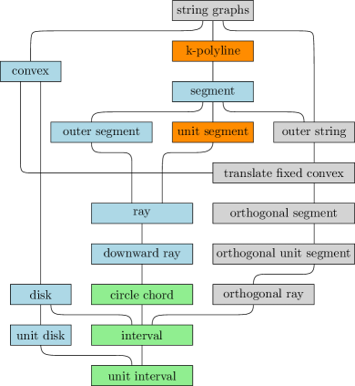
Figure 2: Each box represents a different geometric intersection graph class. Those marked in green can be recognized in polynomial time. Those in blue are known to be $\exists\mathbb{R}$-complete. The ones in gray are NP-complete, and the orange ones are the new results presented in this paper.

Refining the hierarchy.

We see our main contribution in refining the hierarchy of geometric graph classes for which recognition complexity is known. Both unit segments as well as polylines with $k$ bends are natural objects that are well studied in the literature. However, the recognition of the corresponding graph classes was not studied previously. Polylines with an unbounded number of bends are equivalent to strings, while polylines with $0$ bends are just segments. Polylines with $k$ bends thus naturally slot in between strings and segments, and their corresponding graph class is thus also an intermediate class between the class of segment intersection graphs and string graphs, as can be seen in Figure 2. By showing that recognition for polylines with $k$ bends is $\exists\mathbb{R}$-complete for all constant $k$, we see that the switch from $\exists\mathbb{R}$-completeness (segment intersection graphs) to NP-membership (string graphs) really only happens once $k$ is infinite. Similarly, unit segment intersection graphs slot in between segment and ray intersection graphs. Intuitively, recognition of a class intermediate to two classes that are $\exists\mathbb{R}$-hard to recognize should also be $\exists\mathbb{R}$-hard, and our Theorem 1 confirms this intuition in this case.

Large coordinates.

One of the consequences of $\exists\mathbb{R}$-completeness is that there are no short representations of solutions known. Some representable graphs may only be representable by objects with irrational coordinates, or by rational coordinates with nominator and denominator of size at least $2^{2^{n^{c}}}$, for some fixed $c>0$. In other words, the numbers to describe the position might need to be doubly exponentially large [27] for some graphs. For “flexible” objects like polylines, rational solutions can always be obtained by slightly perturbing the representation, however for more “sturdy” objects like unit segments this may not be possible.

Unraveling the broader story.

Given the picture of Figure 2, we wish to start unraveling a deeper story. Namely, we aim to get a better understanding of when geometric recognition problems are $\exists\mathbb{R}$-complete and when they are contained in NP. Figure 2 indicates that $\exists\mathbb{R}$-hardness comes from objects that are complicated enough to avoid a complete combinatorial characterization. Unit interval graphs, interval graphs and circle chord graphs admit such a characterization that in turn can be used to develop a polynomial-time algorithm for their recognition. On the other hand, if the geometric objects are too broad, the recognition problem is in NP. The prime example is string graphs. For string graphs, it is sufficient to know the planar graph given by the intersection pattern of the strings, which is purely combinatorial information that does not care anymore about precise coordinates. Despite the fact that there are graphs that need an exponential number of intersections, it is possible to find a polynomial-size witness [36] and thus we do not have $\exists\mathbb{R}$-hardness. We want to summarize this as: recognition problems are $\exists\mathbb{R}$-complete if the underlying family of geometric objects is at a sweet spot of neither being too simplistic nor too flexible.

When we consider Table 1 we observe two different types of $\exists\mathbb{R}$-complete families. The first type of family encapsulates all rotations $O^{\includegraphics[scale={0.15}]{figures/rotation.pdf}}$ of a given object $O$ (i.e., segments, rays, unit segments etc.). The second type of family contains translates and possibly homothets of geometric objects that have some curvature themselves (i.e., disks and unit disks). However in case we fix a specific object without curvature, i.e., a polygon, and consider all translations of it then the recognition problem also lies in NP [30]. Therefore, broadly speaking, curvature or rotation seem to be properties needed for $\exists\mathbb{R}$-completeness and the lack of it seems to imply NP-membership. We wish to capture one part of this intuition in the following conjecture:

Conjecture A.

Let $O$ be a convex body in the plane with at least two distinct points. Then $\textsc{Recognition}(O^{\includegraphics[scale={0.15}]{figures/rotation.pdf}})$ is $\exists\mathbb{R}$-complete.

We wonder if our intuition on curvature of geometric objects could be generalized as well. It seems plausible that $\textsc{Recognition}(O^{\includegraphics[scale={0.15},page=2]{figures/rotation.pdf}})$ is $\exists\mathbb{R}$-complete if and only if $O$ has curvature.

Restricted geometric graph classes.

A classic way to make an algorithmic problem easier is to consider it only on restricted input. In the context of $\exists\mathbb{R}$ and geometric graph recognition, we would like to mention the work by Schaefer [35], where it is shown that the recognition problem of segments is already $\exists\mathbb{R}$-complete for graphs of bounded degree. We conjecture that the same is true for unit segments and polylines. However, this does not follow from our reductions since we create graphs of unbounded degree.

Conjecture B.

Unit Recognition is $\exists\mathbb{R}$-complete already for graphs of bounded degree.

Once this would be established it would be interesting to find the exact degree threshold when the problem switches from being difficult to being easy.

1.3 Existential Theory of the Reals.

The class of the existential theory of the reals $\exists\mathbb{R}$ (pronounced as ‘ER’) is a complexity class which has gained a lot of interest, specifically within the computational geometry community. To define this class, we first consider the problem ETR, which also stands for Existential Theory of the Reals. In an instance of this problem we are given a sentence of the form

$$\exists x_{1},\ldots,x_{n}\in\mathbb{R}:\Phi(x_{1},\ldots,x_{n}),$$

where $\Phi$ is a well-formed quantifier-free formula consisting of the symbols $\{0,1,x_{1},\ldots,x_{n},+,\cdot,\geq,>,\wedge,\vee,\neg\}$, the goal is to check whether this sentence is true. As an example of an ETR-instance, we could take $\Phi=x\cdot y^{2}+x\geq 0\wedge\neg(y<2x)$. The goal of this instance would be to determine whether there exist real numbers $x$ and $y$ satisfying this formula.

Now the class $\exists\mathbb{R}$ is the family of all problems that admit a polynomial-time many-one reduction to ETR. It is known that

$$\textsf{NP}\subseteq\exists\mathbb{R}\subseteq\textsf{PSPACE}.$$

The first inclusion follows from the definition of $\exists\mathbb{R}$ as follows. Given any Boolean satisfiability formula, we can replace each positive occurrence of a variable $x$ by $x=1$. For example $(x\lor\lnot y)\land(\lnot x\lor z)$ becomes $(x=1\lor\lnot y=1)\land(\lnot x=1\lor z=1)$.

Showing the second inclusion was first done by Canny in his seminal paper [13]. The reason that $\exists\mathbb{R}$ is an important complexity class is that a number of common problems, mainly in computational geometry, have been shown to be complete for this class, see below.

We want to point out that there are some subtleties in the definition of ETR. Since a sentence in ETR can only contain the integers $0$ and $1$, it naively takes $\Theta(n)$ bits to encode a natural number $n$, i.e., $n=1+1+\ldots+1$. However, it is possible to encode $n$ in $O(\log n)$ bits using Horner’s Schema (i.e., $15=1+2\cdot 7=1+2(1+6)=\ldots$). This makes ETR as defined above just as powerful as a definition that would also allow for arbitrary integers encoded in binary. Furthermore, we want to emphasize that the reductions used for defining $\exists\mathbb{R}$ are performed in the word RAM model (or equivalently on a Turing machine), and not on a real Random Access Machine (real RAM) or in the Blum-Shub-Smale model.

The main reason that the complexity class $\exists\mathbb{R}$ gained traction in recent years is the increasing number of important algorithmic problems that are $\exists\mathbb{R}$-complete. Schaefer established the current name and pointed out first that several known NP-hardness reductions actually imply $\exists\mathbb{R}$-completeness [33]. Note that some important reductions that establish $\exists\mathbb{R}$-completeness were done before the class was named.

Problems that have a continuous solution space and non-linear relation between partial solutions are natural candidates to be $\exists\mathbb{R}$-complete. Early examples are related to recognition of geometric structures: points in the plane [29, 42], geometric linkages [34, 1], segment graphs [25, 27], unit disk graphs [28, 21], ray intersection graphs [14], and point visibility graphs [14]. In general, the complexity class is more established in the graph drawing community [26, 16, 35, 18]. Yet, it is also relevant for studying polytopes [31, 17]. There is a series of papers related to Nash-Equilibria [6, 38, 20, 8, 9]. Another line of research studies matrix factorization problems [15, 40, 41, 39]. Other $\exists\mathbb{R}$-complete problems are the Art Gallery Problem [3, 44], covering polygons with convex polygons [2], geometric packing [5] and training neural networks [4, 7].

1.4 Proof Techniques

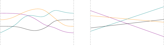
Figure 3: The pseudoline arrangement on the left is combinatorially equivalent to the line arrangement on the right and thus stretchable.

The techniques used in this paper are similar to previous work. In essence, we are reducing from the Stretchability problem. In this problem, we are given a pseudoline arrangement as an input, and the question is whether this arrangement is stretchable (see below for a detailed explanation). Given the initial pseudoline arrangement, we construct a graph. Certain vertices represent the pseudolines, and in any representation of the graph by unit segments or polylines their realizations witness that the pseudolines are stretchable. We use a long cycle surrounding the construction to enforce a certain order on any representation. Furthermore, we use probes to guarantee the desired combinatorial structure. Both general ideas have already been used in different contexts [14].

The main idea to show hardness of PolyLine Recognition is to build a construction where the polylines have to make $k$ bends such that the crucial part has no bends and witnesses the stretchability of the original pseudoline arrangement.

Definition 3 (Pseudoline arrangement).

A pseudoline arrangement $\mathcal{A}$ is a set of $n$ curves that are $x$-monotone. Furthermore, any two curves intersect exactly once and no three curves meet in a single point. We assume that there exist two vertical lines on which each curve starts and ends. No intersections of curves lie on these vertical lines.

Note that the literature sometimes distinguishes between simple and general pseudoline arrangements. For us all the pseudoline arrangements are simple, so we drop the term simple, similarly to how we speak of graphs meaning simple graphs. Further note that line arrangements that are truncated far enough are also pseudoline arrangements.

We say two pseudoline arrangements have the same combinatorics if there exists an isomorphism (bijective and continuous) of the plane that deforms one into the other. It is known that the order in which each pseudoline intersects the remaining pseudolines determines the combinatorial type completely. We say a pseudoline arrangement is stretchable, if there exists a line arrangement with the same combinatorics. Compare to Figure 3.

2 Cycle Representations

In our reduction, we will construct a graph $G$ that contains a cycle. The cycle helps us to enforce a certain structure on any geometric representation of $G$. The arguments in this section merely use that our geometric objects are Jordan arcs whose pairwise intersections consist of a finite number of connected components, and are not specific to either unit segments or polylines.

We first want to introduce some notions about realizations of induced cycles by Jordan arcs. Let $G$ be a graph, and let $C\subseteq V(G)$ be a set of vertices such that the induced graph $G[C]$ is a cycle $(c_{1},\ldots,c_{n})$ of $n\geq 4$ vertices. If we are now given a geometric representation of $G$ as an intersection graph of Jordan arcs, we can define two Jordan curves “tracing” the representation $r(C)$ sufficiently close, one on the inside and one on the outside of $r(C)$. To be precise, by sufficiently close we mean that the curves are close enough to $r(C)$, such that between the two curves no other object $o\not\in r(C)$ starts or ends, no proper crossing of two such other objects occurs, and such that every crossing of another object $o$ with one of the curves implies that $o$ also intersects $r(C)$ within a small $\epsilon$-ball centered at the intersection with the curve. We call the two curves interior boundary curve and exterior boundary curve. See Figure 4 for an illustration.

Figure 4: Top row: The representation $r(C)$ by segments, polylines and strings respectively. Bottom row: The representation of the top row with two boundary curves added. One on the interior and one on the exterior of the representation. From left to right we see unit segments, polylines with one bend and general Jordan arcs. Left: The interior curve traces the Jordan arcs $abcdcdefg$. The exterior curve traces $ababcbcdedefefgfgag$. Middle: The interior curve traces the Jordan arcs $abcdcdef$. The exterior curve traces $ababcdcdefefaf$. Right: The interior curve traces the Jordan arcs $abcdcdcd$. The exterior curve traces $ababcbcdad$.

Observation 4.

The interior boundary curve lies completely within the bounded cell bounded by the exterior boundary curve.

Given either the interior or exterior boundary curve, we can record the order of traced elements, i.e., the order of elements $c\in C$ for which the boundary curve is close to $r(c)$, see Figure 4 for an illustration. This order admits some simple structure, that we describe in the following lemma.

Lemma 5.

Let $C$ be an induced cycle of length $n\geq 4$, and let $b$ be either the interior or exterior boundary curve of $r(C)$. Let $s\in C^{*}$ be the string describing the cyclic order of traced elements of $b$. Then this string can be decomposed into $n$ consecutive parts $s_{1},\ldots,s_{n}$, where in each part $s_{i}$, only the elements $c_{i},c_{i+1}$ occur (note that we take indices modulo $n$).

Proof.

We stretch out the boundary curve horizontally and draw the Jordan arcs it traces on the top of the boundary curve (see Figure 5). Let us now assume that $c_{i}$ appears again on the sequence after $c_{i+2}$ was already seen, but not $c_{i+3}$ yet. Note that the vertices $c_{i+2}$ and $c_{i}$ are not adjacent in $C$, thus their curves are not allowed to intersect. By definition the boundary curve is also not intersected. Thus $c_{i+2}$ is enclosed by $c_{i}$ and the boundary curve and cannot intersect $c_{i+3}$. This is a contradiction, and we thus know that for all $i$, $c_{i}$ can only be seen before $c_{i+2}$ or after $c_{i+3}$ (with all indices taken modulo $n$).

We can thus split the string into $n$ consecutive parts $s_{1},\ldots,s_{n}$ by simply ending part $s_{i}$ whenever $c_{i}$ occurs for the last time. ∎

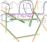
Figure 5: The Jordan arc $c_{i+2}$ is encapsulated by the boundary curve and $c_{i}$ and thus cannot intersect $c_{i+3}$.

Next, we want to argue that for our graph $G$ the realizations of certain vertices of the graph must be contained in some cell.

2.1 Cell Lemma

We start by introducing the notion of a connector. Intuitively, it is just a bunch of vertices that separates an induced cycle from the (connected) rest of the graph.

Definition 6.

Let $G=(V,E)$ be a graph, and $C\subseteq V$ be a set of vertices forming an induced cycle, such that $G[V\setminus C]$ is connected. Let $D\subseteq V\setminus C$ be a set of vertices with the following properties.

• The neighborhood of $C$ is $D$.

• $D$ is an independent set.

• $G[V\setminus D]$ consists of the two connected components, $G[C]$ and $G[V\setminus(C\cup D)]$.

• Each $d\in D$ has exactly one neighbor in $C$, and for any two distinct $d,d^{\prime}\in D$, these neighbors are distinct and non-adjacent.

Then we call the set $D$ connectors of $C$.

This definition is illustrated in Figure 6.

Lemma 7.

Let $C$ be an induced cycle of $G=(V,E)$ with connectors $D$ and $r(V)$ be a geometric representation by Jordan arcs, then either $r(V\setminus(C\cup D))$ lies completely inside the interior curve of $r(C)$ or completely outside the exterior curve of $r(C)$.

Proof.

This follows from the fact that $G[V\setminus(C\cup D)]$ is connected and is not adjacent to the induced cycle $C$. Thus it is also not intersecting the interior or exterior boundary curve. By the Jordan Curve Theorem, the interior (exterior) boundary curve splits the plane in two and thus $G[V\setminus(C\cup D)]$ can only be in one of the two components. ∎

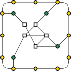
Figure 6: Left: The yellow dots form an induced cycle. The green vertices are connectors of this cycle and the remaining white squares form the rest of the graph. Right: The yellow dots form an induced cycle. The green dots are intersectors of this cycle. The cyclic order $o_{G}$ as used in Lemma 11 is $d_{2},d_{2},d_{1},d_{4},d_{3},d_{1}$, when starting at the top left of the cycle and going clockwise.

2.2 Order Lemma

The aim of this section is to show that certain vertices neighboring an induced cycle also need to intersect this cycle in the same order in any geometric representation. We start with a definition of the setup.

Definition 8.

Let $G=(V,E)$ be a graph, and $C\subset V$ a set of vertices forming an induced cycle. Let $D\subset V\setminus C$ be a set of vertices with the following properties.

• Each $d\in D$ has either one or two neighbors in $C$.

• If $d\in D$ has two neighbors in $C$, these are non-adjacent.

• For any two distinct $d,d^{\prime}\in D$, their neighbors in $C$ are distinct and non-adjacent.

Then we call the set $D$ intersectors of $C$.

This definition is illustrated in Figure 6. We now define two cyclic orders of intersections of intersectors with the cycle. The first order lives in the realm of the graph, while the second one is concerned with a concrete realization. The goal of this section is to prove that these orders are the same.

Definition 9 (Graph Order of Intersectors).

Let $G$ be a graph with $C$ an induced cycle on at least four vertices, and let $D$ be intersectors of $C$. When we travel along the cycle $C$ for one full rotation, we can write down the pairs $(c,d)\in C\times D$, such that $\{c,d\}\in E(G)$. This string of pairs defines the graph order of the intersectors up to a cyclic shift and reflection.

Definition 10 (Geometric Order of Intersectors).

Let $G$ be a graph with $C$ an induced cycle on at least four vertices, and let $D$ be intersectors of $C$. Let $r$ be a realization of $G$ by Jordan arcs and let $b$ be the interior boundary curve of $r(C)$. When we travel along $b$ for one full rotation, we can write down the pairs $(c,d)\in C\times D$ such that $r(d)$ intersects $b$ where $b$ is tracing $r(c)$. From consecutive copies of the same pair we only keep one. This string of pairs defines the geometric order of the intersectors up to a cyclic shift and reflection.

The graph order is illustrated in Figure 6, while the geometric order is illustrated in Figure 7.

Lemma 11.

Let $r$ be a realization of a graph $G$ with an induced cycle $C$ and intersectors $D$. If for every intersection of some $r(d)$ for $d\in D$ with some $r(c)$ for $c\in C$ we have that $r(d)$ also intersects the interior boundary curve $b$ close to that intersection, then the geometric and graph order of the intersectors are the same.

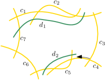
Figure 7: A realization of an induced cycle $C$ (yellow Jordan arcs) and intersectors of $C$ (green Jordan arcs). The cyclic order $o_{r}$ along the interior boundary curve as used in Lemma 11 is here $(c_{5},d_{2}),(c_{7},d_{1}),(c_{2},d_{1})$, when starting at the bottom right and going clockwise (see black arrow).

Proof.

We first claim that every pair $(c,d)$ occurs in both orders exactly once if $\{c,d\}\in E(G)$, and zero times otherwise: In the graph order this holds by definition. Furthermore, the assumption of this lemma guarantees that any pair $(c,d)$ in the graph order of intersectors also occurs in the geometric order of intersectors. We thus only need to show that in the geometric order no pair occurs multiple times. A pair could only occur more than once if there is another pair $(c^{\prime},d^{\prime})$ between these occurrences. However, since $c$ is only crossed by $d$, and no neighbor of $c$ in $C$ is crossed by any intersector, Lemma 5 guarantees that no such pair $(c^{\prime},d^{\prime})$ can occur between the two occurrences of $(c,d)$.

Next, we show that the pairs are also ordered the same way. Since for any two pairs $(c,d),(c^{\prime},d^{\prime})$ in the two vertices $c,c^{\prime}$ are distinct and non-adjacent, Lemma 5 guarantees that the geometric order of the intersectors must respect the ordering of the $c_{i}$ along the cycle. Similarly, the graph order of intersectors must respect this ordering by definition. Thus, the two orders are the same. ∎

Note that the definition of the geometric order and Lemma 11 also work for the exterior boundary curve instead of the interior one.

3 Proofs

In this section, we first show the $\exists\mathbb{R}$-membership parts of Theorems 1 and 2. Then, we prove $\exists\mathbb{R}$-hardness, first for unit segments, then for polylines. The reduction for polylines builds upon the reduction for unit segments and we will only highlight the differences.

3.1 $\exists\mathbb{R}$-Membership

There are two standard ways to establish $\exists\mathbb{R}$-membership. The naive way is to encode the problem at hand as an ETR-formula. The second method describes a real witness and a real verification algorithm, similar as to how one can prove NP-membership using a combinatorial verification algorithm. We describe both approaches.

We describe the naive approach only for unit segments, however a similar technique also easily works for polylines. Let $G=(V,E)$ be a graph. For each vertex $v\in V$, we use four variables $\left\llbracket v1\right\rrbracket,\left\llbracket v2\right\rrbracket,\left\llbracket v3\right\rrbracket,\left\llbracket v4\right\rrbracket$ meant to describe the coordinates of the endpoints of a unit segment realizing $v$. We can construct ETR-formulas unit and intersection that test whether a segment has unit length and whether two segments are intersecting, respectively. The formula $\varphi$ consists of the three parts:

$$\bigwedge_{v\in V}\ \textsc{unit}(\left\llbracket v1\right\rrbracket,\left\llbracket v2\right\rrbracket,\left\llbracket v3\right\rrbracket,\left\llbracket v4\right\rrbracket),$$

$$\bigwedge_{uv\in E}\ \textsc{intersection}(\left\llbracket u1\right\rrbracket,\left\llbracket u2\right\rrbracket,\left\llbracket u3\right\rrbracket,\left\llbracket u4\right\rrbracket,\left\llbracket v1\right\rrbracket,\left\llbracket v2\right\rrbracket,\left\llbracket v3\right\rrbracket,\left\llbracket v4\right\rrbracket),$$

and

$$\bigwedge_{uv\not\in E}\ \lnot\,\textsc{intersection}(\left\llbracket u1\right\rrbracket,\left\llbracket u2\right\rrbracket,\left\llbracket u3\right\rrbracket,\left\llbracket u4\right\rrbracket,\left\llbracket v1\right\rrbracket,\left\llbracket v2\right\rrbracket,\left\llbracket v3\right\rrbracket,\left\llbracket v4\right\rrbracket).$$

The unit formula can be constructed using the formula for the Euclidean norm. To construct the intersection formula it is possible to use the orientation test: The orientation test formula checks whether a given ordered triple of points is oriented clockwise, or counter-clockwise. Using multiple orientation tests on the endpoints of two segments one can determine whether the segments intersect. The orientation test itself can be constructed using a standard determinant test. This finishes the description of the formula $\varphi$ and establishes $\exists\mathbb{R}$-membership.

Although all of these formulas are straightforward to describe, things get a bit lengthy (especially in the case of polylines) and we do hide some details about the precise polynomials. We therefore also wish to describe the second approach using real witnesses and verification algorithms. To use this approach we need to first introduce a different characterization of the complexity class $\exists\mathbb{R}$. Namely, an algorithmic problem is in $\exists\mathbb{R}$ if and only if we can provide a real verification algorithm [19]. A real verification algorithm $A$ for a problem $P$, takes as input an instance $I$ of $P$ and a polynomial-size real-valued witness $w$. $A$ must have the following properties: In case that $I$ is a yes-instance, there exists a $w$ such that $A(I,w)$ returns yes. In case that $I$ is a no-instance $A(I,w)$ will return no, for all possible $w$. Note that this is reminiscent of the definition of NP using a verifier algorithm. There are two subtle differences: The first one is that $w$ is allowed to contain real numbers and discrete values, not only bits. The second difference is that $A$ runs on the real RAM instead of a Turing machine. This is required since a Turing machine is not capable of dealing with real numbers. It is important to note that $I$ itself does not contain any real numbers. We refer to Erickson, Hoog, and Miltzow [19] for a detailed definition of the real RAM.

Given this alternative characterization of $\exists\mathbb{R}$, it is now very easy to establish $\exists\mathbb{R}$-membership of Unit Recognition and PolyLine Recognition: We merely need to describe the witness and the verification algorithm. The witness is a description of the coordinates of the unit segments (or polylines, respectively) realizing the given graph. The verification algorithm merely checks that the correct realizations of vertices intersect one another, and in the case of unit segments, also checks that all segments have the correct length. Note that we sweep many details of the algorithm under the carpet. However, algorithms are much more versatile than formulas and it is a well-established fact that algorithms are capable of all types of elementary operations needed to perform this verification.

3.2 $\exists\mathbb{R}$-Hardness for Unit Segments

This section is dedicated to show $\exists\mathbb{R}$-hardness of Unit Recognition by a reduction from Stretchability.

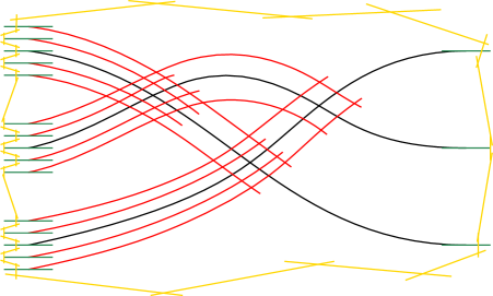
Figure 8: A pseudoline arrangement (black), enhanced with probes (red), connectors (green) and a cycle (yellow).

We present the reduction in three steps. First, we show how we construct a graph $G$ from a pseudoline arrangement $\mathcal{A}$. Then we show completeness, i.e., we show that if $\mathcal{A}$ is stretchable then $G$ can be represented using unit segments. At last, we will show soundness, i.e., we show that if $G$ can be represented using unit segments then $\mathcal{A}$ is stretchable. For this part we will use the lemmas from Section 2.

Construction.

Given a pseudoline arrangement $\mathcal{A}$ of $n$ pseudolines as defined in Definition 3, we construct a graph $G$ by enhancing the arrangement $\mathcal{A}$ with additional Jordan arcs. Then we define $G$ to be the intersection graph of the pseudolines (which are also Jordan arcs) and all our added arcs. See Figure 8 for an illustration.

First, we add so called probes to our pseudolines. A probe of depth $k$ of pseudoline $\ell$ is a Jordan arc which starts on the left vertical line, and follows $\ell$ closely through the arrangement until it has intersected $k$ other pseudolines (and all probes of that other pseudoline which reach that intersection). For each pseudoline $\ell$, we add $2(n-1)$ probes: Above and below $\ell$ we add one probe each for each depth $1\leq k\leq n-1$. This gives a total of $p:=2n(n-1)$ probes in the graph $G$. The probes are sorted according to their depth, with the probes of smallest depth situated closest to $\ell$. Note that so far we have added $n+p$ arcs. We now create connectors for each probe and pseudoline. A connector is a short Jordan arc added to the left and/or right end of another arc. For probes, we only add connectors at the left end, while pseudolines get connectors at both ends. Note that we thus add $d:=2n+p$ connectors. Finally, we add Jordan arcs forming cycle of length $2d+6$ around the current arrangement. At the left and right end, this cycle is placed in such a way that every second arc of the cycle intersects a connector, in the correct order. The eight additional arcs of the cycle are used to connect the left and right side of the cycle, using four arcs on the top and four arcs on the bottom.

We denote the collection of all those arcs (including the pseudolines) as the enhanced pseudoline arrangement. The graph $G$ is given by the intersection graph of this arrangement. Note that $G$ could also be described purely combinatorially, and it can be constructed in polynomial time.

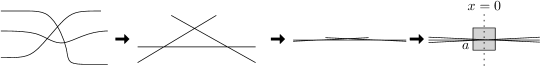
Figure 9: Left to Right: pseudoline arrangement $\mathcal{A}$; stretched line arrangement $\mathcal{L}$, squeezed line arrangement to have small slopes; squeezed to have all intersections in a box of side length $a$.

Completeness.

This paragraph is dedicated to show that if $\mathcal{A}$ is stretchable then $G$ is realizable by unit segments. We assume that $\mathcal{A}$ is stretchable and show how to place each unit segment realizing $G$. We denote the segments representing the pseudolines, probes, connectors, and the cycle by important segments, probe segments, connector segments and cycle segments.

$\mathcal{A}$ being stretchable implies that there exists a combinatorially equivalent line arrangement $\mathcal{L}$. The arrangement $\mathcal{L}$ can be compressed (scaled down along the vertical axis) such that the slopes of all lines lie in some small interval $[-a,a]$, for say $a=1/20$. Additionally, we can move and scale $\mathcal{L}$ even more to ensure that all intersection points lie in the square $[-a,a]^{2}$. See Figure 9 for an illustration.

We now truncate all the lines of $\mathcal{L}$ to get unit segments that have the same intersection pattern as the corresponding lines. The truncation is performed symmetrically around the vertical line $x=0$. The resulting unit segments are our important segments.

For the next step we consider an important segment $s$ and construct its corresponding probe segments. We place all probe segments parallel to its important segment $s$, with sufficiently small distance to $s$ and to each other. The probe segments are placed as far towards the left as possible, while still reaching the intersections of important segments they need to reach. Since by construction of the scaled line arrangement $\mathcal{L}$ all intersections lie within $[-a,a]^{2}$ and the probes can only go until there, each probe segment and its corresponding important segment are almost collinear but shifted by roughly $0.5$ longitudinally See Figure 10 for an illustration of the placement of the probe segments.

Next we need to describe the placement of the connector segments. Note that on the right side, we only have important segments. We add all the connector segments in such a way that they lie on the same line as the important/probe segment they attach to. The connectors can overlap with the segments they attach to for a large part, since the first intersection of any probe and important segments only occurs in the square $[-a,a]^{2}$. This allows us to place our connectors such that all connectors on the left (right) side of the drawing end at the same left (right) $x$-coordinate.

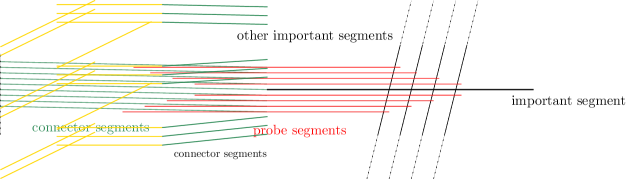
Figure 10: Given $\mathcal{L}$, we can construct the probe segments and connector segments using unit segments. The connector segments are illustrated slightly tilted, for the purpose of readability. They should be parallel to the segment that they connect to.

Figure 11: We can place all the connector segments correctly on the left and on the right using a simple sawtooth pattern.

Finally, we can draw the cycle segments. For this, we simply make a sawtooth pattern on the left and on the right. See Figure 11 for an illustration. In our sawtooth pattern, every second cycle segment is horizontal, and all other cycle segments are parallel. The horizontal segments attach to the connector segments. As the important segments all have a very small slope, we can never run into a situation where two horizontal cycle segments would be too far away from each other to be connected. We connect the left and right sawtooth patterns to close the cycle, using our eight additional cycle segments.

Soundness.

This paragraph is dedicated to show that $G$ being realizable using unit segments implies that $\mathcal{A}$ is stretchable. We thus assume there exists a realization $r$ of $G$ by unit segments. Similarly to the last paragraph, we denote the vertices representing the pseudolines, probes, connectors, and the cycle by important vertices $I$, probe vertices $P$, connector vertices $D$, and cycle vertices $C$.

Note that $C$ forms an induced cycle in $G$ and $D$ are connectors of $C$ as in Definition 6 (thus motivating the name). By Lemma 7, $r(C)$ splits the plane into two cells, and $r(I\cup P)$ is contained completely in one of these two cells. Without loss of generality, we assume $r(I\cup P)$ is contained in the inner (bounded) cell, however all following arguments would also work with the outer cell. Thus, every segment in $r(D)$ intersects the cycle $r(C)$ from the inside, i.e., it intersects the interior boundary curve. We can thus apply Lemma 11, and get that $r(D)$ is ordered along the interior boundary curve of $C$ in the same way (up to cyclic shift and reflection) as it is in our enhanced pseudoline arrangement as described in the construction of $G$. Specifically, we know that the important segments and probe segments are ordered as in our enhanced pseudoline arrangement, see Figure 8.

We now claim that the arrangement of the important segments $r(I)$ is combinatorially equivalent to $\mathcal{A}$. Thus, extending these segments to lines yields a combinatorially equivalent line arrangement. To see this, we pick three pseudolines $\ell$, $a$, and $b$, such that $\ell$ intersects $a$ before $b$ when going from left to right in $\mathcal{A}$. We prove that in our realization $r$, the unit segment $r(\ell)$ must also intersect the segment $r(a)$ before $r(b)$. The orientation of the unit segments $r(\ell)$ is determined as follows: $r(\ell)$ intersects two connectors $d_{1},d_{2}$ that intersect $r(C)$ in two different unit segments. One of these unit segments $c$ (intersected by connector $d_{1}$) is two segments away from a unit segment that intersects a connector that intersects a probe of $\ell$. We then orient $r(\ell)$ in the direction such that the intersection with $d_{1}$ occurs before the intersection with $d_{2}$. Note that since $d_{1}$ and $d_{2}$ do not intersect, this order is uniquely defined. Furthermore, simply rotating or mirroring the representation does not change this order.

Now, let us suppose for the purpose of a contradiction that $r(\ell)$ intersects $r(b)$ before $r(a)$. Let us consider the following curves:

• the outermost probe segments of $\ell$,

• their connector segments,

• a part of the interior boundary curve of the cycle segments, and

• the important segment $b$.

Since these segments form an induced cycle in the graph $G$, these segments bound a cell $E$. In this cycle, $\ell$ and its connector segment $d_{1}$ (the one attaching to the cycle between the probes) form a chord, thus their representations split $E$ into two parts $E_{1},E_{2}$. See Figure 12 for an illustration. Note that $r(\ell)$ must be oriented from the end contained in $E$ towards the other end, since the intersection of $r(d_{1})$ and $r(\ell)$ lies in $E$, but the intersection of $r(d_{2})$ and $r(\ell)$ cannot. Since we assume that $r(\ell)$ intersects $r(b)$ before $r(a)$, the intersection of $r(a)$ and $r(\ell)$ thus lies outside of $E$.

We consider the two probe segments $p,q$ of $\ell$, which correspond to the intersection with $a$. These segments are attached to the cycle between the outermost probe segments of $\ell$, and $\ell$ itself. Furthermore, $p$ and $q$ are not intersecting any segment bounding $E_{1}$ or $E_{2}$, in particular not $r(b)$. Thus the probe segments $p$ and $q$ are both completely contained in the interior of $E_{1}$ and $E_{2}$, respectively. However, $r(a)$ can intersect the interior of only one of $E_{1}$ and $E_{2}$, but not both, since $r(a)$ and $r(\ell)$ are line segments and their single intersection is assumed to lie outside of $E$. Since both $p$ and $q$ must intersect $r(a)$, we arrive at the desired contradiction. We thus conclude that $\mathcal{A}$ is stretchable, finishing the proof of Theorem 1.

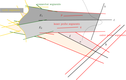
Figure 12: Suppose for the purpose of contradiction that $\ell$ intersects $a$ after $b$. Then the important segment $a$ can only intersect one of the cells $E_{1}$ and $E_{2}$. However, $E_{1}$ and $E_{2}$ contain a segment that $a$ intersects in its interior. A contradiction.

3.3 $\exists\mathbb{R}$-Hardness for Polylines

In this section, we study polylines with $k$ bends and we assume $k>0$ is a fixed constant. Specifically, we will show that PolyLine Recognition is $\exists\mathbb{R}$-complete.

The proof for polylines works very similarly to the proof for unit segments. Since the family of polylines is a strict superset of the family of unit segments, most of our additional work is on the soundness of the proof. To be able to ensure soundness, our construction of the graph $G$ will make sure that the polylines realizing the pseudolines cannot contain any bends in some region encoding the pseudoline arrangement $\mathcal{A}$ in any realization of $G$. With this property, the argument for soundness (as in the proof of Theorem 1) will carry over straightforwardly.

Construction.

As in the construction for unit segments, we enhance our arrangement $\mathcal{A}$ of $n$ pseudolines using additional Jordan arcs, and let our graph $G$ be the intersection graph of the enhanced arrangement.

To create the enhanced arrangement, we first create the frame: We create $2k+2$ vertical chains of $c\cdot n^{2}$ line segments, for some $c$ sufficiently large. We call the set of segments forming the $i$-th such vertical chain $C_{i}$, for $i=1\dots,2k+2$, numbered from left to right. We then connect these vertical chains by two horizontal chains, one at the top and one at the bottom. All of the segments forming these chains are called frame segments, and they together bound $2k+1$ bounded cells. We call the leftmost such cell the canvas.

We now place our pseudoline arrangement in the canvas. For every pseudoline $p$, we first introduce a parallel twin pseudoline $p^{\prime}$ closely below $p$. Since $\mathcal{A}$ is assumed to be simple, every pseudoline has the same intersection pattern with all the other pseudolines as its twin.

Next, we introduce probes from the left of our pseudoline arrangement, as we did in the proof of Theorem 1. Note that every pair of twin pseudolines shares one set of probes. We attach the probes as well as the pseudolines and their twins to $C_{1}$ using connector arcs, making sure that each connector intersects a unique arc of $C_{1}$, and that none of these arcs are intersecting.

We now want to weave the pseudolines and their twins through $C_{2},\ldots,C_{2k+1}$. To do this, we split each set $C_{i}$ into $n$ lanes $L_{i,1},\ldots,L_{i,n}$: A lane is a set of three consecutive arcs of $C_{i}$. The lanes $L_{i,j}$ are pairwise disjoint, and no arc of any lane $L_{i,j}$ may intersect an arc of a lane $L_{i,j^{\prime}}$. Note that the lanes are ordered along $C_{i}$ with $L_{i,1}$ being the topmost lane and $L_{i,n}$ the bottommost. We also number our pseudolines from $p_{1}$ to $p_{n}$ by their order at the right end of the arrangement, from top to bottom. For every pseudoline $p_{j}$, we now extend $p_{j}$ and its twin $p_{j}^{\prime}$ as follows: For each even $i$, $p_{j}$ goes through the top arc of the lane $L_{i,j}$, and for each odd $i$, it goes through the bottom arc of $L_{i,j}$. The twin $p_{j}^{\prime}$ is extended in the opposite way, going through the top arc of $L_{i,j}$ if $i$ is odd, and through the bottom arc for $i$ even.

At the very end, at $C_{2k+2}$, we use a connector arc to attach each pseudoline $p_{j}$ to the top element of $L_{2k+2,j}$, and its twin $p_{j}^{\prime}$ to the bottom element. This whole construction is illustrated in Figure 13.

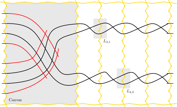
Figure 13: A doubled pseudoline arrangement (black) enhanced for $k=2$ with probes (red), connectors (green) and the frame (yellow). The shaded region is the canvas.

Completeness.

Given a line arrangement $\mathcal{L}$ combinatorially equivalent to $\mathcal{A}$, we want to show that $G$ is realizable by polylines. It is easy to see that given $\mathcal{L}$, the canvas and its contents (probes, connectors, pseudolines, and pseudoline twins) can be realized even with line segments (i.e., using $0$ bends), as we argued already in the proof of Theorem 1. The only remaining difficulty is to argue that the extended pseudolines weaving through $C_{2},\ldots,C_{2k+1}$ and finally attaching to $C_{2k+2}$ can be realized using at most $k$ bends per pseudoline and twin.

Since between every two lanes $L_{i,j}$ and $L_{i,j+1}$ there is at least one polyline that is not part of any lane, we can make the distance between these lanes arbitrarily large. We thus only need to show that for a single pair $p_{j}$, $p_{j}^{\prime}$, we can weave the polylines through $L_{2,j},\ldots,L_{2k+2,j}$. The construction is illustrated in Figure 14: The two polylines exit the canvas in parallel. Then, going from left to right, we first use all bends of $p_{j}$, leaving its twin straight. After having gone through $L_{2,j},\ldots,L_{k+2,j}$, we leave $p_{j}$ straight and use the bends of the twin to go through the remaining lanes $L_{k+3,j},\ldots,L_{2k+1,j}$ and to have the right ordering to attach to $C_{2k+2}$ using a connector.

Figure 14: Weaving the two copies (dashed and dotted) of a pseudoline through the $2k$ chords with at most $k$ bends per polyline. Illustrated for $k=2$.

Soundness.

Given a realization of the graph $G$ with polylines, we want to argue that $\mathcal{A}$ is stretchable. To achieve this, we first prove some structural lemmas about all realizations of $G$.

Lemma 12.

In every realization $r(G)$, the polylines realizing all probes, pseudolines, and internal vertices of $C_{2},\ldots,C_{2k+1}$ must lie on the same side of the boundary curves given by the cycle bounded by $C_{1}$ and $C_{2k+2}$.

Proof.

The induced subgraph of this set of vertices is connected. The connectors attaching them to the outermost cycle together with the outermost segments of $C_{2},\ldots,C_{2k+1}$ thus form a set of connectors as defined in Definition 6. Thus the lemma follows from Lemma 7 immediately. ∎

We again assume without loss of generality that all these elements lie in the interior (bounded) cell bounded by the outermost cycle. We now know that for every pair of consecutive chords $C_{i},C_{i+1}$, any element $r(v)$ that intersects the cycle bounded by these chords must also intersect the interior boundary curve of that cycle. We can thus apply Lemma 11 to these cycles to enforce the ordering of crossings along them. From this, similarly as in the proof of soundness for unit segments (note that that proof did not use the fact that the line segments were unit), we wish to get that the arrangement obtained by picking either $r(p_{j})$ or $r(p_{j}^{\prime})$ for every $j\in[n]$ restricted to the canvas has the same combinatorial structure as $\mathcal{A}$. However, for this it remains to be shown that at least one of $r(p_{j})$ and $r(p_{j}^{\prime})$ must be a straight line within the canvas. To show this, we first show that the two polylines $r(p_{j})$ and $r(p_{j}^{\prime})$ must cross often:

Lemma 13.

Within the cell enclosed by the interior boundary curve of the cycle enclosed by two consecutive sets $C_{i},C_{i+1}$, for $2\leq i\leq 2k+1$, each $r(p_{j})$ and $r(p_{j}^{\prime})$ must cross.

Proof.

By Lemma 11 and by construction of $G$, the geometric order of $r(p_{j})$ and $r(p_{j}^{\prime})$ along the interior boundary curve of the cell bounded by $C_{i}$ and $C_{i+1}$ must be alternating (non-nesting). Thus, the two polylines $r(p_{j})$ and $r(p_{j}^{\prime})$ must cross within this cell. ∎

Lemma 14.

Let $c,d$ be two polylines that intersect in exactly $t$ points $i_{1},\ldots,i_{t}$, with both polylines visiting the intersection points in this order. Then $c$ and $d$ have at least $t-1$ bends in total between the first and the last intersection.

Proof.

It is easy to see that there must be at least one bend between any two consecutive intersection points. See Figure 15 for an illustration. ∎

Figure 15: It is easy to see that the two polylines must have at least one bend between the two intersection points.

We now finally get our desired lemma:

Lemma 15.

At least one of $r(p_{j})$ and $r(p_{j}^{\prime})$ is a straight line within the canvas.

Proof.

The two twin polylines must have at least $2k$ intersection points that occur in the same order along the two twin: to find these points, we pick one per cell enclosed between $C_{i},C_{i+1}$ for $2\leq i\leq 2k+1$ as guaranteed by Lemma 13. Thus by Lemma 14, the two polylines have at least $2k-1$ bends in total outside of the canvas. This implies that at least one of them is straight inside the canvas. ∎

We conclude that $\mathcal{A}$ must be stretchable, finishing the proof of Theorem 2.

References

- [1] Zachary Abel, Erik Demaine, Martin Demaine, Sarah Eisenstat, Jayson Lynch, and Tao Schardl. Who needs crossings? Hardness of plane graph rigidity. In 32nd International Symposium on Computational Geometry (SoCG 2016), pages 3:1–3:15. Schloss Dagstuhl - Leibniz-Zentrum für Informatik, 2016. doi:10.4230/LIPIcs.SoCG.2016.3.
- [2] Mikkel Abrahamsen. Covering Polygons is Even Harder. In Nisheeth K. Vishnoi, editor, 2021 IEEE 62nd Annual Symposium on Foundations of Computer Science (FOCS), pages 375–386, 2022. doi:10.1109/FOCS52979.2021.00045.
- [3] Mikkel Abrahamsen, Anna Adamaszek, and Tillmann Miltzow. The art gallery problem is -complete. Journal of the ACM, 69(1):4:1–4:70, 2022. doi:10.1145/3486220.
- [4] Mikkel Abrahamsen, Linda Kleist, and Tillmann Miltzow. Training neural networks is -complete. In NeurIPS 2021, pages 18293–18306, 2021. URL: https://proceedings.neurips.cc/paper/2021/hash/9813b270ed0288e7c0388f0fd4ec68f5-Abstract.html.
- [5] Mikkel Abrahamsen, Tillmann Miltzow, and Nadja Seiferth. Framework for -completeness of two-dimensional packing problems. In 2020 IEEE 61st Annual Symposium on Foundations of Computer Science (FOCS), pages 1014–1021, 2020. doi:10.1109/FOCS46700.2020.00098.
- [6] Marie Louisa Tølbøll Berthelsen and Kristoffer Arnsfelt Hansen. On the computational complexity of decision problems about multi-player Nash equilibria. Theory of Computing Systems, 66(3):519–545, 2022. doi:10.1007/s00224-022-10080-1.
- [7] Daniel Bertschinger, Christoph Hertrich, Paul Jungeblut, Tillmann Miltzow, and Simon Weber. Training fully connected neural networks is -complete. CoRR, abs/2204.01368, 2022. To appear at NeurIPS 2024. arXiv:2204.01368.
- [8] Vittorio Bilò and Marios Mavronicolas. A catalog of -complete decision problems about Nash equilibria in multi-player games. In 33rd Symposium on Theoretical Aspects of Computer Science (STACS 2016). Schloss Dagstuhl - Leibniz-Zentrum für Informatik, 2016. doi:10.4230/LIPIcs.STACS.2016.17.
- [9] Vittorio Bilò and Marios Mavronicolas. -complete decision problems about symmetric Nash equilibria in symmetric multi-player games. In 34th Symposium on Theoretical Aspects of Computer Science (STACS 2017). Schloss Dagstuhl - Leibniz-Zentrum für Informatik, 2017. doi:10.4230/LIPIcs.STACS.2017.13.
- [10] Csaba Biró, Édouard Bonnet, Dániel Marx, Tillmann Miltzow, and Pawel Rzazewski. Fine-grained complexity of coloring unit disks and balls. Journal of Computational Geometry, 9(2):47–80, 2018. doi:10.20382/jocg.v9i2a4.
- [11] Marthe Bonamy, Édouard Bonnet, Nicolas Bousquet, Pierre Charbit, Panos Giannopoulos, Eun Jung Kim, Pawel Rzazewski, Florian Sikora, and Stéphan Thomassé. EPTAS and subexponential algorithm for maximum clique on disk and unit ball graphs. Journal of the ACM, 68(2):9:1–9:38, 2021. doi:10.1145/3433160.
- [12] Kellogg S. Booth and George S. Lueker. Testing for the consecutive ones property, interval graphs, and graph planarity using -tree algorithms. Journal of Computer and System Sciences, 13(3):335–379, 1976. doi:10.1016/S0022-0000(76)80045-1.
- [13] John Canny. Some algebraic and geometric computations in PSPACE. In Proceedings of the Twentieth Annual ACM Symposium on Theory of Computing, STOC ’88, page 460–467, New York, NY, USA, 1988. Association for Computing Machinery. doi:10.1145/62212.62257.
- [14] Jean Cardinal, Stefan Felsner, Tillmann Miltzow, Casey Tompkins, and Birgit Vogtenhuber. Intersection Graphs of Rays and Grounded Segments. Journal of Graph Algorithms and Applications, 22(2):273–294, 2018. doi:10.7155/jgaa.00470.
- [15] Dmitry Chistikov, Stefan Kiefer, Ines Marusic, Mahsa Shirmohammadi, and James Worrell. On Restricted Nonnegative Matrix Factorization. In Ioannis Chatzigiannakis, Michael Mitzenmacher, Yuval Rabani, and Davide Sangiorgi, editors, 43rd International Colloquium on Automata, Languages, and Programming (ICALP 2016), volume 55 of Leibniz International Proceedings in Informatics (LIPIcs), pages 103:1–103:14, Dagstuhl, Germany, 2016. Schloss Dagstuhl – Leibniz-Zentrum für Informatik. doi:10.4230/LIPIcs.ICALP.2016.103.
- [16] Michael G. Dobbins, Linda Kleist, Tillmann Miltzow, and Paweł Rzążewski. -Completeness and Area-Universality. In Andreas Brandstädt, Ekkehard Köhler, and Klaus Meer, editors, Graph-Theoretic Concepts in Computer Science (WG 2018), volume 11159 of Lecture Notes in Computer Science, pages 164–175. Springer, 2018. doi:10.1007/978-3-030-00256-5_14.
- [17] Michael Gene Dobbins, Andreas Holmsen, and Tillmann Miltzow. A universality theorem for nested polytopes. arXiv, 1908.02213, 2019.
- [18] Jeff Erickson. Optimal curve straightening is -complete. arXiv:1908.09400, 2019.
- [19] Jeff Erickson, Ivor van der Hoog, and Tillmann Miltzow. Smoothing the gap between NP and ER. In 2020 IEEE 61st Annual Symposium on Foundations of Computer Science (FOCS), pages 1022–1033, 2020. doi:10.1109/FOCS46700.2020.00099.
- [20] Jugal Garg, Ruta Mehta, Vijay V. Vazirani, and Sadra Yazdanbod. -completeness for decision versions of multi-player (symmetric) Nash equilibria. ACM Transactions on Economics and Computation, 6(1), 2018. doi:10.1145/3175494.
- [21] Ross Kang and Tobias Müller. Sphere and Dot Product Representations of Graphs. Discrete & Computational Geometry, 47(3):548–569, 2012. doi:10.1007/s00454-012-9394-8.
- [22] Jan Kratochvíl. String graphs. I. The number of critical nonstring graphs is infinite. Journal of Combinatorial Theory. Series B, 52(1):53–66, 1991. doi:10.1016/0095-8956(91)90090-7.
- [23] Jan Kratochvíl. String graphs. II. Recognizing string graphs is NP-hard. Journal of Combinatorial Theory. Series B, 52(1):67–78, 1991. doi:10.1016/0095-8956(91)90091-W.
- [24] Jan Kratochvíl and Jiří Matoušek. NP-hardness results for intersection graphs. Commentationes Mathematicae Universitatis Carolinae, 30(4):761–773, 1989.
- [25] Jan Kratochvíl and Jiří Matoušek. Intersection graphs of segments. Journal of Combinatorial Theory. Series B, 62(2):289–315, 1994. doi:10.1006/jctb.1994.1071.
- [26] Anna Lubiw, Tillmann Miltzow, and Debajyoti Mondal. The complexity of drawing a graph in a polygonal region. Journal of Graph Algorithms and Applications, 26(4):421–446, 2022. doi:10.7155/jgaa.00602.
- [27] Jiří Matoušek. Intersection graphs of segments and . ArXiv 1406.2636, 2014.
- [28] Colin McDiarmid and Tobias Müller. Integer realizations of disk and segment graphs. Journal of Combinatorial Theory. Series B, 103(1):114–143, 2013. doi:10.1016/j.jctb.2012.09.004.
- [29] Nicolai Mnëv. The universality theorems on the classification problem of configuration varieties and convex polytopes varieties. In Topology and geometry – Rohlin seminar, pages 527–543, 1988.
- [30] Tobias Müller, Erik Jan van Leeuwen, and Jan van Leeuwen. Integer representations of convex polygon intersection graphs. SIAM Journal on Discrete Mathematics, 27(1):205–231, 2013. doi:10.1137/110825224.
- [31] Jürgen Richter-Gebert and Günter M. Ziegler. Realization spaces of 4-polytopes are universal. Bulletin of the American Mathematical Society, 32(4):403–412, 1995.
- [32] Alexandre Rok and Bartosz Walczak. Outerstring graphs are -bounded. SIAM Journal on Discrete Mathematics, 33(4):2181–2199, 2019. doi:10.1137/17M1157374.
- [33] Marcus Schaefer. Complexity of some geometric and topological problems. In David Eppstein and Emden R. Gansner, editors, Graph Drawing, pages 334–344, Berlin, Heidelberg, 2010. Springer Berlin Heidelberg. doi:10.1007/978-3-642-11805-0_32.
- [34] Marcus Schaefer. Realizability of Graphs and Linkages, pages 461–482. Thirty Essays on Geometric Graph Theory. Springer, 2013. doi:10.1007/978-1-4614-0110-0_24.
- [35] Marcus Schaefer. Complexity of geometric k-planarity for fixed k. Journal of Graph Algorithms and Applications, 25(1):29–41, 2021. doi:10.7155/jgaa.00548.
- [36] Marcus Schaefer, Eric Sedgwick, and Daniel Štefankovič. Recognizing string graphs in NP. Journal of Computer and System Sciences, 67(2):365–380, 2003. Special Issue on STOC 2002. doi:10.1016/S0022-0000(03)00045-X.
- [37] Marcus Schaefer and Daniel Štefankovič. Decidability of string graphs. Journal of Computer and System Sciences, 68(2):319–334, 2004. Special Issue on STOC 2001. doi:10.1016/j.jcss.2003.07.002.
- [38] Marcus Schaefer and Daniel Štefankovič. Fixed points, Nash equilibria, and the existential theory of the reals. Theory of Computing Systems, 60(2):172–193, Feb 2017. doi:10.1007/s00224-015-9662-0.
- [39] Marcus Schaefer and Daniel Štefankovič. The complexity of tensor rank. Theory of Computing Systems, 62(5):1161–1174, 2018. doi:10.1007/s00224-017-9800-y.
- [40] Yaroslav Shitov. A universality theorem for nonnegative matrix factorizations. ArXiv 1606.09068, 2016.
- [41] Yaroslav Shitov. The complexity of positive semidefinite matrix factorization. SIAM Journal on Optimization, 27(3):1898–1909, 2017. doi:10.1137/16M1080616.
- [42] Peter W. Shor. Stretchability of Pseudolines is NP-Hard. In Peter Gritzmann and Bernd Sturmfels, editors, Applied Geometry And Discrete Mathematics, volume 4 of DIMACS Series in Discrete Mathematics and Theoretical Computer Science, pages 531–554, 1991. doi:10.1090/dimacs/004/41.
- [43] Jeremy Spinrad. Recognition of circle graphs. Journal of Algorithms. Cognition, Informatics and Logic, 16(2):264–282, 1994. doi:10.1006/jagm.1994.1012.
- [44] Jack Stade. Complexity of the boundary-guarding art gallery problem. CoRR, abs/2210.12817, 2022. doi:10.48550/arXiv.2210.12817.