Quadratic discontinuous Galerkin finite element methods for the unilateral contact problem

Abstract.

In this article, we employ discontinuous Galerkin (DG) methods for the finite element approximation of the frictionless unilateral contact problem using quadratic finite elements over simplicial triangulation. We first establish an optimal a priori error estimates under the appropriate regularity assumption on the exact solution $\boldsymbol{u}$. Further, we analyze a posteriori error estimates in the DG norm wherein, the reliability and efficiency of the proposed a posteriori error estimator is addressed. The suitable construction of discrete Lagrange multiplier $\boldsymbol{\lambda_{h}}$ and some intermediate operators play a key role in developing a posteriori error analysis. Numerical results presented on uniform and adaptive meshes illustrate and confirm the theoretical findings.

1. Introduction

The numerical analysis of contact problems arising in the various physical phenomena plays a substantial role in understanding processes and effects in natural sciences. From mathematical point of view, contact problems are modeled as variational inequalities which play an essential role in solving class of various non-linear boundary value problems arising in the physical fields. Much of the mathematical basis of modeling and detailed understanding of contact problems within the framework of variational inequality can be found in the book by Kikuchi and Oden [40]. Among the contact problems, the unilateral contact represented by the frictionless Signorini model simulates the contact between a linear elastic body and a rigid foundation. The Signorini problem is basically studied as a prototype for elliptic variational inequality (EVI) of the first kind. In the underlying variational inequality, the non-linearity condition in the weak formulation is incorporated in a closed and convex set on which the formulation is posed. This contact problem was formulated by Signorini (see [47]) followed by that Fichera in [27] carried out an extensive study of Signorini problem in the context of EVI’s. Subsequently, many researchers have done plenty of work in modeling the contact problems. The study of a priori error analysis for unilateral contact problem using conforming linear finite elements can be found in [4, 30, 40]. Resorting to the higher order finite elements provide more accurate computed solution [22], compared to linear elements. Contrarily, less literature is available for the same. The article [9] exploits the two non-conforming quadratic approximation to the Signorini problem and derive a priori error estimates. In order to quantify the discretization errors, a posteriori error estimators act as an indispensable tool. In article [36], the authors constructed a positivity preserving interpolation operator to derive a reliable and efficient residual based a posteriori error estimators for Signorini problem using linear finite elements. Further, in the article [57], the a posteriori error analysis is carried out without using the positivity preserving interpolation operator. A residual based a posteriori error estimator of conforming linear finite element method for the Signorini problem is developed in [42] using a suitable construction of the quasi discrete contact force density. There is hardly any work available in the literature towards the a posteriori error analysis of quadratic finite element methods for the Signorini problem.

Unlike the standard finite element method, the discontinuous Galerkin methods introduced by Reed and Hill [45] work with the space of trial functions which are only piecewise continuous. These methods are well known for their flexibility for hp adaptivity. The discontinuous property permits the usage of general meshes with hanging nodes. In addition to this, its property to incorporate the non-homogeneous boundary condition in the weak formulation greatly increases the accuracy and robustness of any boundary condition implementation. Consequently, DG methods have been applied to study several linear and non-linear partial differential equations. We refer to [23, 35, 44, 46] and the references therein for the comprehensive study of DG methods.

In the past decades, DG methods are extensively used to solve variational inequalities. In the article [54], the ideas discussed in [3] were extended to deduce an optimal a priori error estimates of DG methods for obstacle and simplified Signorini problem. Followed by that in article [55] and [53], DG formulations for Signorini problem and quasi static contact problem are derived using linear elements and optimal a priori error estimates are established for these methods. The articles [31, 33, 56, 29] addressed a posteriori error control for obstacle problem using DG methods. The study of a posteriori error estimates on adaptive mesh for Signorini problem using discontinuous linear elements was dealt in [32]. Therein, the authors carried out the analysis by defining the continuous Lagrange multiplier as a functional on $\boldsymbol{H^{\frac{1}{2}}}(\Gamma_{C})$. In comparison to [32], M. Walloth in the article [51] discussed the a posteriori error analysis of DG methods for Signorini problem which relies on the construction of quasi discrete contact force density. In this article, we provide a rigorous analysis for the DG discretization with quadratic polynomials to Signorini problem, therein both a priori and a posteriori error analysis are discussed. We followed the approach shown in the article [32] and defined continuous Lagrange multiplier on $\boldsymbol{H^{-\frac{1}{2}}}(\Gamma_{C})$. The interpolation operator $\boldsymbol{\pi_{h}}$ and $\boldsymbol{\beta_{h}}$ (defined in equation (3.5) and equation (5.1), respectively) is suitably constructed to exhibit the desired properties which are later used to define discrete counter part of Lagrange multiplier.

The outline of the article is as follows: In Section 1, we state the classical and variational formulation of the Signorini problem. In addition to this, we define an auxiliary functional on the space $\boldsymbol{H^{\frac{1}{2}}}(\Gamma_{C})$ pertaining to the exact solution and complimentarity conditions on the contact region. We introduce some prerequisite notations and preliminary results in Section 2. Therein, we also define the discrete counterpart of the continuous problem on closed, convex non-empty subset of a quadratic finite element space, couple of interpolation operators and discuss several DG formulations. Section 3 is dedicated to derive an optimal a priori error estimates with respect to the regularity of the exact solution, followed by that in Section 4 we introduce the discrete counterpart $\boldsymbol{\lambda_{h}}$ of Lagrange multiplier $\boldsymbol{\lambda}$ on a suitable space. Next, we derive the sign properties of $\boldsymbol{\lambda_{h}}$ which play a key role in the subsequent analysis. In order to deal with the discontinuous finite elements we construct an enriching map which connects DG functions with conforming finite elements and preserves constraints on discrete functions. Section 5 is devoted to unified a posteriori error analysis for the various DG methods wherein, we discuss the reliablity and efficiency of a posteriori error estimator. Finally in Section 6, the theoretical results are corroborated by two numerical experiments addressing contact of a linear elastic body with the rigid obstacle. Therein, the optimal convergence of the error on uniform mesh and the convergence behavior of error estimator over adaptive mesh are demonstrated for two DG methods namely, SIPG and NIPG.

2. Signorini Contact Problem

Let $\Omega$ represents a bounded, polygonal linear elastic body in $\mathbb{R}^{2}$ with Lipschitz boundary $\partial\Omega=\Gamma$ which is partitioned into three mutually disjoint, relatively open sets; the Dirichlet boundary $\Gamma_{D}$, the Neumann boundary $\Gamma_{N}$ and the potential contact boundary $\Gamma_{C}$ with $meas(\Gamma_{D})>0$ and $\overline{\Gamma}_{C}\subset\Gamma\leavevmode\nobreak\ \backslash\leavevmode\nobreak\ \overline{\Gamma}_{D}$.

Let $\boldsymbol{u}:\Omega\rightarrow\mathbb{R}^{2}$ denote the displacement vector. Then, the linearized strain tensor

(2.1) $$\boldsymbol{\varepsilon}(\boldsymbol{u}):=\dfrac{1}{2}\big{(}\boldsymbol{\nabla}\boldsymbol{u}+(\boldsymbol{\nabla}\boldsymbol{u})^{\boldsymbol{T}}\big{)},$$

and stress tensor

(2.2) $$\boldsymbol{\sigma}(\boldsymbol{u}):=\mathcal{C}\boldsymbol{\varepsilon}(\boldsymbol{u}),$$

belong to $\boldsymbol{\mathbb{S}}^{2}$ which is the space of second order real symmetric tensors on $\mathbb{R}^{2}$ with the inner product $\boldsymbol{\psi}:\boldsymbol{\chi}=\psi_{ij}\chi_{ij}$ and the norm $|\boldsymbol{\psi}|=(\boldsymbol{\psi}:\boldsymbol{\psi})^{\frac{1}{2}}\leavevmode\nobreak\ \leavevmode\nobreak\ \forall\leavevmode\nobreak\ \boldsymbol{\psi},\boldsymbol{\chi}\in\boldsymbol{\mathbb{S}}^{2}$ . In the relation (2.2), $\mathcal{C}$ denotes the bounded, symmetric and positive definite fourth order elasticity tensor defined on $\Omega\times\mathbb{S}^{2}\longrightarrow\mathbb{S}^{2}$. In particular, for a homogeneous and isotropic elastic body, the stress tensor obeys Hooke’s law and is explicitly given by

$$\mathcal{C}\boldsymbol{\varepsilon}(\boldsymbol{u}):=2\mu\boldsymbol{\varepsilon}(\boldsymbol{u})+\lambda(\text{tr}\boldsymbol{\varepsilon}(\boldsymbol{u}))\textbf{Id},$$

where, $\mu>0$ and $\lambda>0$ denote the Lam$\acute{e}$’s parameter and Id is an identity matrix of order 2.

Throughout this article, the vector valued functions are identified with the bold symbols whereas the scalar valued functions are written in usual way. Let $\boldsymbol{n}$ denotes the outward unit normal vector to $\Gamma$, then for any vector $\boldsymbol{v}$, we decompose its normal and tangential component as $v_{n}:=\boldsymbol{v}\cdot\boldsymbol{n}$ and $\boldsymbol{v_{\tau}}:=\boldsymbol{v}-v_{n}\boldsymbol{n}$, respectively. Analogously, for any tensor valued function $\boldsymbol{\Psi}$ in $\boldsymbol{\mathbb{S}}^{2}$, we denote $\Psi_{n}:=\boldsymbol{\Psi}\boldsymbol{n}\cdot\boldsymbol{n}$ and $\boldsymbol{\Psi_{\tau}}:=\boldsymbol{\Psi}\boldsymbol{n}-\Psi_{n}\boldsymbol{n}$ as its normal and tangential component, respectively. Further, we will require the following decomposition formula

(2.3) $$(\boldsymbol{\Psi}\boldsymbol{n})\cdot\boldsymbol{v}=\Psi_{n}v_{n}+\boldsymbol{\Psi_{\tau}}\cdot\boldsymbol{v}_{\tau}.$$

In the following static contact model problem, the linear elastic body lying on a rigid foundation is subjected to volume force of density $\boldsymbol{f}$ in $\Omega$, surface traction force $\boldsymbol{g}$ on Neumann boundary together with unilateral contact condition on $\Gamma_{C}$. The pointwise formulation of the contact problem is described below in subsection (2.1).

2.1. Strong formulation of Signorini problem:

Find the displacement vector $\boldsymbol{u}:\Omega\rightarrow\mathbb{R}^{2}$ satisfying the equations (2.4)-(2.7),

(2.4) $$\boldsymbol{-div}\leavevmode\nobreak\ \leavevmode\nobreak\ \boldsymbol{\sigma}(\boldsymbol{u}) =\boldsymbol{f}\leavevmode\nobreak\ \leavevmode\nobreak\ \leavevmode\nobreak\ \leavevmode\nobreak\ \textit{in}\leavevmode\nobreak\ \Omega,$$

(2.5) $$\boldsymbol{u} =\boldsymbol{0}\leavevmode\nobreak\ \leavevmode\nobreak\ \leavevmode\nobreak\ \leavevmode\nobreak\ \textit{on}\leavevmode\nobreak\ \Gamma_{D},$$

(2.6) $$\boldsymbol{\sigma}(\boldsymbol{u})\boldsymbol{n} =\boldsymbol{g}\leavevmode\nobreak\ \leavevmode\nobreak\ \leavevmode\nobreak\ \leavevmode\nobreak\ \textit{on}\leavevmode\nobreak\ \Gamma_{N},$$

(2.7) $$\begin{split}\left.\begin{aligned} u_{n}&\leq 0,\leavevmode\nobreak\ \leavevmode\nobreak\ \sigma_{n}(\boldsymbol{u})\leq 0\\ u_{n}\sigma_{n}(\boldsymbol{u})&=0,\leavevmode\nobreak\ \leavevmode\nobreak\ \boldsymbol{\sigma_{\tau}}(\boldsymbol{u})=0\end{aligned}\right\}on\leavevmode\nobreak\ \leavevmode\nobreak\ \Gamma_{C},\end{split}$$

where $\boldsymbol{f}\in[L^{2}(\Omega)]^{2}$ and $\boldsymbol{g}\in[L^{2}(\Gamma_{N})]^{2}$. The equilibrium equation in which volume force of density $\boldsymbol{f}$ acts in $\Omega$ is described in (2.4). The equation $\eqref{1.5}$ depicts that the displacement field vanishes on Dirichlet boundary, thus the body is clamped on $\Gamma_{D}$. On the contact boundary $\Gamma_{C}$, the relation (2.7) constitutes the non-penetration condition that evokes the contact stresses in the direction of the constraints. In addition, the contact of elastic body and deformable foundation is assumed to be frictionless, henceforth the frictional stresses $\boldsymbol{\sigma_{\tau}}(\boldsymbol{u})$ are assumed to be zero (see Figure 2.1).

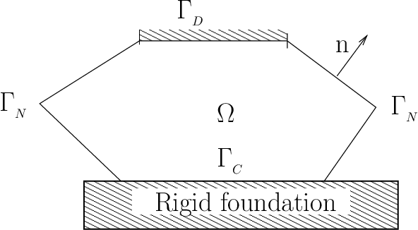
Figure 2.1. Physical setting of Signorini problem

In the subsequent analysis, we will make a constant use of Sobolev spaces $H^{m}(\Omega)$ which is endowed with the following norm $\|{v}\|_{H^{m}(\Omega)}:=\bigg{(}\underset{0\leq|\alpha|\leq m}{\sum}\|\partial^{\alpha}{v}\|^{2}_{L^{2}(\Omega)}\bigg{)}^{\frac{1}{2}}$ and semi norm $|{v}|_{H^{m}(\Omega)}:=\bigg{(}\underset{|\alpha|=m}{\sum}\|\partial^{\alpha}{v}\|^{2}_{L^{2}(\Omega)}\bigg{)}^{\frac{1}{2}},$ respectively. Here, $\alpha=(\alpha_{1},\alpha_{2})$ represents the multi index in $\mathbb{N}^{2}$ and the symbol $\partial^{\alpha}$ refers to the partial derivative of $v$ defined as $\partial^{\alpha}v:=\frac{\partial^{|\alpha|}v}{\partial x^{\alpha_{1}}\partial y^{\alpha_{2}}}$. Furthermore, for a non-integer positive number $s$, we define fractional order Sobolev space $H^{s}(\Omega)$ as

$$H^{s}(\Omega):=\bigg{\{}\boldsymbol{v}\in H^{\gamma}(\Omega):\dfrac{{\lvert{v}(x)-{v}(y)\rvert}}{{\lvert x-y\rvert}^{\theta+1}}\in L^{p}(\Omega\times\Omega)\bigg{\}},$$

where $s=\leavevmode\nobreak\ \gamma\leavevmode\nobreak\ +\leavevmode\nobreak\ \theta$, $\gamma$ and $\theta$ denotes the greatest integer and fractional part of $s$, respectively. In addition, for any vector $\boldsymbol{v}=(v^{1},v^{2})\in\boldsymbol{H^{m}}(\Omega)$ = $[H^{m}(\Omega)]^{2}$, we define the product norm as $\|\boldsymbol{v}\|_{\boldsymbol{H^{m}}(\Omega)}:=\bigg{(}\sum\limits_{i=1}^{2}\|{v^{i}}\|^{2}_{{H^{m}(\Omega)}}\bigg{)}^{\frac{1}{2}}$ and semi norm $|\boldsymbol{v}|_{\boldsymbol{H^{m}}(\Omega)}:=\bigg{(}\sum\limits_{i=1}^{2}|{v^{i}}|^{2}_{{H^{m}(\Omega)}}\bigg{)}^{\frac{1}{2}}$.

In unilateral contact problem, the contact between two bodies occurs on the part of the boundary thus the trace operator plays an important role. We refer to [15, 40] for the detailed understanding of trace operators. Let the trace of $\boldsymbol{H^{1}}(\Omega)$ functions restricted to boundary $\Gamma_{C}$ is denoted by $\boldsymbol{H^{\frac{1}{2}}}(\Gamma_{C})$ which is equipped with the norm

$$\|\boldsymbol{v}\|_{\boldsymbol{H^{\frac{1}{2}}}(\Gamma_{C})}:=\bigg{(}\|\boldsymbol{v}\|^{2}_{\boldsymbol{L^{2}}(\Gamma_{C})}+\int_{\Gamma_{C}}\int_{\Gamma_{C}}\dfrac{\lvert{\boldsymbol{v}(x)-\boldsymbol{v}(y)\rvert^{2}}}{{\lvert x-y\rvert}^{2}}\leavevmode\nobreak\ dxdy\bigg{)}^{\frac{1}{2}},\leavevmode\nobreak\ \quad\leavevmode\nobreak\ \boldsymbol{v}\in{\boldsymbol{H^{\frac{1}{2}}}(\Gamma_{C})}.$$

Further, let $\boldsymbol{\gamma_{c}}:\boldsymbol{H^{1}}(\Omega)\rightarrow\boldsymbol{H^{\frac{1}{2}}}(\Gamma_{C})$ be the trace map. The continuity and surjectivity of the trace map guarantees existence of continuous right inverse which we denote by $\boldsymbol{\hat{\gamma}_{c}}:\boldsymbol{H^{\frac{1}{2}}}(\Gamma_{C})\rightarrow\boldsymbol{H^{1}}(\Omega)$ such that $\boldsymbol{{\gamma_{c}}\leavevmode\nobreak\ o\leavevmode\nobreak\ \hat{\gamma}_{c}}=\text{identity}$. Denote the space $\boldsymbol{H^{-\frac{1}{2}}}(\Gamma_{C})$ as the dual space of $\boldsymbol{H^{\frac{1}{2}}}(\Gamma_{C})$ endowed with the norm

$$\|\boldsymbol{T}\|_{\boldsymbol{H^{-\frac{1}{2}}}(\Gamma_{C})}:=\underset{\boldsymbol{v}\leavevmode\nobreak\ \in\leavevmode\nobreak\ \boldsymbol{H^{\frac{1}{2}}}(\Gamma_{C}),\leavevmode\nobreak\ \boldsymbol{v}\neq 0}{\text{sup}}\frac{\boldsymbol{T}\boldsymbol{(v)}}{\leavevmode\nobreak\ \leavevmode\nobreak\ \|\boldsymbol{v}\|_{\boldsymbol{H^{\frac{1}{2}}}(\Gamma_{C})}}\leavevmode\nobreak\ \forall\leavevmode\nobreak\ \boldsymbol{T}\in{\boldsymbol{H^{-\frac{1}{2}}}(\Gamma_{C})},$$

and let $\langle\cdot,\cdot\rangle_{c}$ denotes the duality pairing between the space $\boldsymbol{H^{-\frac{1}{2}}}(\Gamma_{C})$ and $\boldsymbol{H^{\frac{1}{2}}}(\Gamma_{C})$ i.e. $\langle\boldsymbol{T},\boldsymbol{w}\rangle_{c}:=\boldsymbol{T}(\boldsymbol{w})\leavevmode\nobreak\ \forall\leavevmode\nobreak\ \boldsymbol{T}\in\boldsymbol{H^{-\frac{1}{2}}}(\Gamma_{C})$ and $\boldsymbol{w}\in\boldsymbol{H^{\frac{1}{2}}}(\Gamma_{C})$. In the further sections, the conventional symbols are used without any specific explanation.

2.2. Variational Setting

In this subsection, we introduce the weak formulation of the Signorini problem which is represented by a variational inequality due to the constraints on the potential contact boundary. For this purpose, let us introduce the Hilbert space $\boldsymbol{{V}}$ for the displacement fields as

$$\boldsymbol{{V}}:=\{\boldsymbol{v}\in\boldsymbol{H^{1}}(\Omega):\boldsymbol{v}=\boldsymbol{0}\leavevmode\nobreak\ \text{on}\leavevmode\nobreak\ \Gamma_{D}\},$$

and let $\boldsymbol{{V}^{{}^{\prime}}}$ denotes its topological dual space endowed with the usual norm. Further, in order to incorporate the unilateral contact conditions on $\Gamma_{C}$ we define a non-empty, closed convex set of admissible displacements as

$$\boldsymbol{{K}}:=\{\boldsymbol{v}\in\boldsymbol{{V}}:v_{n}\leq 0\leavevmode\nobreak\ \text{on}\leavevmode\nobreak\ \Gamma_{C}\}.$$

Exploiting the relation $\sigma_{n}(\boldsymbol{u})(v_{n}-u_{n})\geq 0\leavevmode\nobreak\ \forall\leavevmode\nobreak\ \boldsymbol{v}\in\boldsymbol{{K}}\leavevmode\nobreak\ \text{on}\leavevmode\nobreak\ \Gamma_{C}$ and using integration by parts, we derive the following variational formulation: find a displacement field $\boldsymbol{u}\in\boldsymbol{{K}}$ such that

(2.8) $$a(\boldsymbol{u},\leavevmode\nobreak\ \boldsymbol{v}-\boldsymbol{u})\geq L(\boldsymbol{v}-\boldsymbol{u})\leavevmode\nobreak\ \qquad\forall\leavevmode\nobreak\ \boldsymbol{v}\in\boldsymbol{{K}},$$

where the continuous, $\boldsymbol{{V}}$-elliptic bilinear form $a(\cdot,\leavevmode\nobreak\ \cdot)$ and the continuous linear functional $L(\cdot)$ are defined as

$$a(\boldsymbol{w},\boldsymbol{v}):=\int_{\Omega}\boldsymbol{\sigma}(\boldsymbol{w}):\boldsymbol{\varepsilon}(\boldsymbol{v})\leavevmode\nobreak\ \boldsymbol{dx}\leavevmode\nobreak\ \leavevmode\nobreak\ \leavevmode\nobreak\ \quad\forall\leavevmode\nobreak\ \boldsymbol{w},\boldsymbol{v}\in\boldsymbol{{V}}$$

and

$$\leavevmode\nobreak\ \leavevmode\nobreak\ \leavevmode\nobreak\ \leavevmode\nobreak\ \leavevmode\nobreak\ \leavevmode\nobreak\ L(\boldsymbol{v}):=\int_{\Omega}\boldsymbol{f}\cdot\boldsymbol{v}\leavevmode\nobreak\ \boldsymbol{dx}+\int_{\Gamma_{N}}\boldsymbol{g}\cdot\boldsymbol{v}\leavevmode\nobreak\ \boldsymbol{ds}\leavevmode\nobreak\ \leavevmode\nobreak\ \leavevmode\nobreak\ \quad\forall\leavevmode\nobreak\ \boldsymbol{v}\in\boldsymbol{{V}}.$$

The existence and uniqueness of the solution of the variational inequality (2.8) follows from the well known theorem of Lions and Stampacchia [4, 41]. Following the approach of the article [32], we define Lagrange multiplier $\boldsymbol{\lambda}\in\boldsymbol{H^{-\frac{1}{2}}}(\Gamma_{C})$ which reflects the residual of $\boldsymbol{u}$ with respect to continuous variational formulation (2.8).

Lemma 2.1.

Let $\boldsymbol{u}$ be the solution of the variational formulation (2.8). Then, there exists a continuous linear map

(2.9) $$\langle\boldsymbol{\lambda},\boldsymbol{v}\rangle_{c}:=L(\boldsymbol{\hat{\gamma}_{c}}(\boldsymbol{v}))-a(\boldsymbol{u},\boldsymbol{\hat{\gamma}_{c}}(\boldsymbol{v}))\leavevmode\nobreak\ \quad\forall\leavevmode\nobreak\ \boldsymbol{v}\leavevmode\nobreak\ \in\leavevmode\nobreak\ \boldsymbol{H^{\frac{1}{2}}}(\Gamma_{C}).\leavevmode\nobreak\ \leavevmode\nobreak\ \leavevmode\nobreak\ \leavevmode\nobreak\ \leavevmode\nobreak\$$

In addition, it holds that

(2.10) $$\langle\boldsymbol{\lambda},\leavevmode\nobreak\ \boldsymbol{{\gamma}_{c}}(\boldsymbol{v})\rangle_{c}=L(\boldsymbol{v})-a(\boldsymbol{u},\boldsymbol{v})\leavevmode\nobreak\ \quad\forall\leavevmode\nobreak\ \boldsymbol{v}\in\boldsymbol{{V}},$$

and

(2.11) $$\langle\boldsymbol{\lambda},\leavevmode\nobreak\ \boldsymbol{{\gamma}_{c}}(\boldsymbol{v})-\boldsymbol{{\gamma}_{c}}(\boldsymbol{u})\rangle_{c}\leq\boldsymbol{0}\leavevmode\nobreak\ \quad\forall\leavevmode\nobreak\ \boldsymbol{v}\in\boldsymbol{{K}}.$$

For any $\boldsymbol{v}=(v^{1},v^{2})=(v^{1},0)+(0,v^{2})\in\boldsymbol{{V}}$, we will make use of the following representation of Lagrange multiplier $\boldsymbol{\lambda}=(\lambda^{1},\lambda^{2})$ in each of its component $\langle\boldsymbol{\lambda},\boldsymbol{v}\rangle_{c}=\langle\lambda^{1},v^{1}\rangle+\langle\lambda^{2},v^{2}\rangle$ as follows

(2.12) $$\langle\lambda^{1},v^{1}\rangle:=L((v^{1},0))-a(\boldsymbol{u},(v^{1},0));$$

(2.13) $$\langle\lambda^{2},v^{2}\rangle:=L((0,v^{2}))-a(\boldsymbol{u},(0,v^{2}));$$

In the last equations (2.12) and (2.13), $\langle\cdot,\cdot\rangle$ refers to the duality pairing between $H^{-\frac{1}{2}}(\Gamma_{C})$ and $H^{\frac{1}{2}}(\Gamma_{C})$.

3. Discrete Problem

3.1. Basic Preliminaries and Definitions

In this section, we recall some basic notations which will be useful in developing the subsequent analysis.

• $\mathcal{T}_{h}$ := regular simplical triangulation of domain $\Omega$,

• $K$:= an element in $\mathcal{T}_{h}$,

• $\mathcal{V}_{K}$ := set of all vertices of the triangle $K$,

• $\mathcal{M}_{K}$ := set of midpoints of the triangle $K$,

• $\mathcal{V}_{h}$ := set of all vertices of $\mathcal{T}_{h}$,

• $\mathcal{M}_{h}$ := set of all midpoint of edges in $\mathcal{T}_{h}$,

• $\mathcal{V}_{e}$ := set of two vertices of edge $e$.

• $\mathcal{M}_{e}$ := midpoint of edge $e$.

• $\mathcal{E}_{h}$ := set of all edges of $\mathcal{T}_{h}$,

• $\mathcal{E}_{h}^{i}$ := set of all interior edges of $\mathcal{T}_{h}$,

• $\mathcal{E}_{h}^{D}$:= set of all edges lying on $\Gamma_{D}$,

• $\mathcal{E}_{h}^{C}$:= set of all edges lying on $\Gamma_{C}$,

• $\mathcal{E}_{h}^{0}$ := $\mathcal{E}_{h}^{i}\cup\mathcal{E}_{h}^{D}$,

• $\mathcal{T}_{h}^{C}$ := set of all triangles $K$ such that $\partial K\cap\Gamma_{C}$ is non-empty.

• $\mathcal{E}_{K}^{C}$:= set of contact edges of the triangle $K\in\mathcal{T}_{h}^{C}$.

• $\mathcal{M}_{K}^{C}$:= set of midpoint of the edges $e\in\mathcal{E}_{K}^{C}$.

• $\mathcal{V}_{h}^{D}$:= set of all vertices lying on $\overline{\Gamma}_{D}$,

• $\mathcal{M}_{h}^{D}$:= set of midpoints of edges lying on $\Gamma_{D}$,

• $\mathcal{V}_{h}^{N}$:= set of all vertices lying on ${\Gamma}_{N}$,

• $\mathcal{M}_{h}^{N}$:= set of midpoints of edges lying on $\Gamma_{N}$,

• $\mathcal{V}_{h}^{C}$:= set of all vertices lying on $\overline{\Gamma}_{C}$,

• $\mathcal{M}_{h}^{C}$:= set of midpoints of edges lying on $\Gamma_{C}$,

• $\mathcal{E}_{p}$:= set of all edges sharing the node $p$,

• $\mathcal{T}_{p}$:= set of all triangles sharing the node $p$,

• $\mathcal{T}_{e}$:= set of all triangles sharing the edge $e$,

• $h_{K}$ := diameter of the triangle $K$,

• $h$:= max $\{h_{K}:K\in\mathcal{T}_{h}\}$,

• $h_{e}$:= length of an edge $e$,

• $P_{k}(K)$ denotes the space of polynomials of degree $\leq k$ defined on $K$ where $0\leq k\in\mathbb{Z}$,

• $|S|$ denotes the cardinality of the set $S$,

• $X^{{}^{\prime}}$ := dual space of a Banach space $X$.

In order to formulate the discontinuous Galerkin methods for the weak formulation $\eqref{weak1}$ conveniently, we define the following broken Sobolev space

$$\boldsymbol{H^{1}}(\Omega,\mathcal{T}_{h}):=\{\boldsymbol{v}\in\boldsymbol{L^{2}}(\Omega)|\leavevmode\nobreak\ \boldsymbol{v}_{K}:=\boldsymbol{v}|_{K}\in\boldsymbol{H^{1}}(K)\leavevmode\nobreak\ \forall\leavevmode\nobreak\ K\leavevmode\nobreak\ \in\leavevmode\nobreak\ \mathcal{T}_{h}\},$$

with the broken Sobolev norm $\|\boldsymbol{v}\|^{2}_{\boldsymbol{h}}=\underset{K\in\mathcal{T}_{h}}{\sum}\|\boldsymbol{v}\|^{2}_{\boldsymbol{H^{1}}(K)}\leavevmode\nobreak\ \forall\leavevmode\nobreak\ \boldsymbol{v}\in\boldsymbol{H^{1}}(\Omega,\mathcal{T}_{h})$.

For a scalar valued function $w\in{H^{1}}(\Omega,\mathcal{T}_{h})$, vector valued function $\boldsymbol{v}\in\boldsymbol{H^{1}}(\Omega,\mathcal{T}_{h})$ and tensor valued function $\boldsymbol{\phi}\in[{H^{1}}(\Omega,\mathcal{T}_{h})]^{2\times 2}$ which are double valued across the inter element boundary $e\in\mathcal{E}_{h}^{i}$, the jumps and averages across the edge $e$ are defined as

$$\{\hskip-3.0pt\{w\}\hskip-3.0pt\} :=\dfrac{w|_{K_{1}}+w|_{K_{2}}}{2},\leavevmode\nobreak\ \leavevmode\nobreak\ \leavevmode\nobreak\ [\hskip-1.5pt[w]\hskip-1.5pt]:=w|_{K_{1}}\boldsymbol{n_{1}}+w|_{K_{2}}\boldsymbol{n_{2}};$$

$$\{\hskip-3.0pt\{\boldsymbol{v}\}\hskip-3.0pt\} :=\dfrac{\boldsymbol{v}|_{K_{1}}+\boldsymbol{v}|_{K_{2}}}{2},\leavevmode\nobreak\ \leavevmode\nobreak\ \leavevmode\nobreak\ \leavevmode\nobreak\ [\hskip-1.5pt[\boldsymbol{v}]\hskip-1.5pt]:=\boldsymbol{v}|_{K_{1}}\otimes\boldsymbol{n_{1}}+\boldsymbol{v}|_{K_{2}}\otimes\boldsymbol{n_{2}};$$

$$\{\hskip-3.0pt\{\boldsymbol{\phi}\}\hskip-3.0pt\} :=\dfrac{\boldsymbol{\phi}|_{K_{1}}+\boldsymbol{\phi}|_{K_{2}}}{2},\leavevmode\nobreak\ \leavevmode\nobreak\ \leavevmode\nobreak\ [\hskip-1.5pt[\boldsymbol{\phi}]\hskip-1.5pt]:=\boldsymbol{\phi}|_{K_{1}}\boldsymbol{n_{1}}+\boldsymbol{\phi}|_{K_{2}}\boldsymbol{n_{2}};$$

where the edge $e$ is shared by two contiguous elements $K_{1}$ and $K_{2}$, wherein $\boldsymbol{n_{1}}$ is the outward unit normal vector pointing from $K_{1}$ to $K_{2}$ and $\boldsymbol{n_{2}}=-\boldsymbol{n_{1}}$. Further, for $\boldsymbol{x},\boldsymbol{y}\in\mathbb{R}^{2}$, the dyadic product $\boldsymbol{x}\otimes\boldsymbol{y}\in\mathbb{R}^{2\times 2}$ is defined as $(\boldsymbol{x}\otimes\boldsymbol{y})_{ij}=x_{i}y_{j}$. For the convenience, we also define the jump and averages on the boundary edge $e\in\mathcal{E}_{h}^{b}$ as

$$\{\hskip-3.0pt\{w\}\hskip-3.0pt\} :=w,\leavevmode\nobreak\ \leavevmode\nobreak\ \leavevmode\nobreak\ \leavevmode\nobreak\ \leavevmode\nobreak\ \leavevmode\nobreak\ \leavevmode\nobreak\ \leavevmode\nobreak\ \leavevmode\nobreak\ [\hskip-1.5pt[w]\hskip-1.5pt]:=w\boldsymbol{n_{e}};$$

$$\{\hskip-3.0pt\{\boldsymbol{v}\}\hskip-3.0pt\} :=\boldsymbol{v},\leavevmode\nobreak\ \leavevmode\nobreak\ \leavevmode\nobreak\ \leavevmode\nobreak\ \leavevmode\nobreak\ \leavevmode\nobreak\ \leavevmode\nobreak\ \leavevmode\nobreak\ \leavevmode\nobreak\ \leavevmode\nobreak\ [\hskip-1.5pt[\boldsymbol{v}]\hskip-1.5pt]:=\boldsymbol{v}\otimes\boldsymbol{n_{e}};$$

$$\{\hskip-3.0pt\{\boldsymbol{\phi}\}\hskip-3.0pt\} :=\boldsymbol{\phi},\leavevmode\nobreak\ \leavevmode\nobreak\ \leavevmode\nobreak\ \leavevmode\nobreak\ \leavevmode\nobreak\ \leavevmode\nobreak\ \leavevmode\nobreak\ \leavevmode\nobreak\ \leavevmode\nobreak\ [\hskip-1.5pt[\boldsymbol{\phi}]\hskip-1.5pt]:=\boldsymbol{\phi}\boldsymbol{n_{e}};$$

where $K\in\mathcal{T}_{h}$ is such that $e\subset\partial K$ and $\boldsymbol{n_{e}}$ is the unit normal on the edge $e$ pointing outside $K$. Hereafter, the notations $\boldsymbol{\varepsilon}_{h}(\boldsymbol{v})$ and $\boldsymbol{\sigma}_{h}(\boldsymbol{v})$ are defined by the following relation $\boldsymbol{\varepsilon}_{h}(\boldsymbol{v}):=\boldsymbol{\varepsilon}(\boldsymbol{v})$ and $\boldsymbol{\sigma}_{h}(\boldsymbol{v}):=\boldsymbol{\sigma}(\boldsymbol{v})$ on any triangle $K\in\mathcal{T}_{h}$. Finally the notation $X\lesssim Y$ means there exists a positive generic constant $C$ such that $X\leq CY$.

For the discretization, we use discontinuous quadratic finite element space associated with the simplicial triangulation $\mathcal{T}_{h}$ which is defined as follows

$$\boldsymbol{{V}_{h}}:=\bigg{\{}\boldsymbol{v_{h}}\in\boldsymbol{L^{2}}(\Omega):\leavevmode\nobreak\ \boldsymbol{v_{h}}|_{K}\in[P_{2}(K)]^{2}\leavevmode\nobreak\ \leavevmode\nobreak\ \forall\leavevmode\nobreak\ K\leavevmode\nobreak\ \in\leavevmode\nobreak\ \mathcal{T}_{h}\bigg{\}}.$$

Further, incorporating the unilateral condition in the form of integral constraints, we define the discrete counterpart of the set of admissible displacements $\boldsymbol{{K}}$ as

$$\boldsymbol{{K}_{h}}:=\bigg{\{}\boldsymbol{v_{h}}=(v_{h}^{1},v_{h}^{2})\in\boldsymbol{{V}_{h}}:\int_{e}v_{hn}\leavevmode\nobreak\ ds\leq 0\leavevmode\nobreak\ \forall\leavevmode\nobreak\ e\in\mathcal{E}_{h}^{C}\bigg{\}}.$$

In order to incorporate unilateral contact condition in conforming setting, one needs to enforce non-penetration condition $u_{hn}\leq 0$ everywhere on $\Gamma_{C}$ but the major drawback of this model arises in numerically implementing it. This motivates us to enforce the non-penetration condition in the form of integral constraints. For the ease of analysis, the further study is carried presuming the following assumptions (A) and (B).
Assumption (A) The outward unit normal vector to $\Gamma_{C}$ is constant and for simplicity we set it to be $\boldsymbol{e_{1}}$ where $\boldsymbol{e_{1}}$ and $\boldsymbol{e_{2}}$ denotes the standard ordered basis functions of $\mathbb{R}^{2}$. Thus, the discrete set $\boldsymbol{{K}_{h}}$ reduces to

$$\boldsymbol{{K}_{h}}=\bigg{\{}\boldsymbol{v_{h}}=(v_{h}^{1},v_{h}^{2})\in\boldsymbol{{V}_{h}}:\int_{e}v^{1}_{h}\leavevmode\nobreak\ ds\leq 0\leavevmode\nobreak\ \forall\leavevmode\nobreak\ e\in\mathcal{E}_{h}^{C}\bigg{\}}.$$

Assumption (B) Each triangle $K\in\mathcal{T}^{C}_{h}$ has exactly one potential contact boundary edge.

Remark 3.1.

In the view of assumption (A), it can be easily verified that $\langle\lambda^{2},v^{2}\rangle=0$ for any $\boldsymbol{v}=(v^{1},v^{2})\in\boldsymbol{V}$ using equation (2.13) and the continuous variational inequality (2.8).

In this work, we also require a quadratic conforming finite element space $\boldsymbol{{V}_{c}}=\boldsymbol{{V}_{h}}\cap\boldsymbol{{V}}$ associated with the triangulation $\mathcal{T}_{h}$. Next, we revisit the famous Cl$\acute{e}$ment approximation result [15, Section 4.8, Pg. 122] which will be helpful in further analysis.

Lemma 3.2.

Let $\boldsymbol{v}\in\boldsymbol{{V}}$. Then, there exists $\boldsymbol{v_{h}}\in\boldsymbol{{V}_{c}}$ such that the following estimate holds on any triangle $K\in\mathcal{T}_{h}$

$$\|\boldsymbol{v}-\boldsymbol{v_{h}}\|_{\boldsymbol{H^{l}}(K)}\lesssim h^{1-l}_{K}\|\boldsymbol{v_{h}}\|_{\boldsymbol{H^{1}}(\mathcal{T}_{K})},\leavevmode\nobreak\ \leavevmode\nobreak\ l=0,1,$$

where $\mathcal{T}_{K}$ refers to the set of triangles $\tilde{K}\in\mathcal{T}_{h}$ such that $\overline{\tilde{K}}\cap\overline{K}\neq\emptyset$.

Next, we state the discrete trace and inverse inequalities [15, 22] which will be frequently used in the convergence analysis ahead.

• Discrete trace inequality: For all $K\in\mathcal{T}_{h}$ and $e\subset\partial K$, the following inequality holds for all $\boldsymbol{v}\in\boldsymbol{H^{1}}(K)$.

$$\|\boldsymbol{v}\|^{2}_{\boldsymbol{L^{2}}(e)}\lesssim h^{-1}_{e}\|\boldsymbol{v}\|^{2}_{\boldsymbol{L^{2}}(K)}+h_{e}|\boldsymbol{v}|^{2}_{\boldsymbol{H^{1}}(K)}.$$

• Inverse inequalities: For all $K\in\mathcal{T}_{h}$ and $e\subset\partial K$, the inequalities

  $$\lVert\boldsymbol{v_{h}}\rVert_{\boldsymbol{L^{2}}{(e)}} \lesssim h_{e}^{-\frac{1}{2}}\lVert\boldsymbol{v_{h}}\rVert_{\boldsymbol{L^{2}}(K)},$$

  $$\lVert\nabla\boldsymbol{v_{h}}\rVert_{\boldsymbol{L^{2}}{(K)}} \lesssim h_{K}^{-1}\lVert\boldsymbol{v_{h}}\rVert_{\boldsymbol{L^{2}}(K)},$$

hold for any $\boldsymbol{v_{h}}$ in the discrete space $\boldsymbol{{V}_{h}}$.

3.2. DG Formulation

This subsection is devoted to state various DG formulations for the continuous variational inequality (2.8). For the sake of brievity, we first list the bilinear forms $\mathcal{A}_{h}(\cdot,\cdot)$ corresponding to well known DG methods for the contact problem. We refer to article [55] for the complete derivations of these DG formulations. To this end, let $\boldsymbol{r_{o}}$ and $\boldsymbol{r_{e}}$ denotes the global and local lifting operators [3], respectively. The various DG methods are listed as follows:

• SIPG method [2, 55]:

  $$\hskip 8.53581pt\mathcal{A}_{h}^{(1)}(\boldsymbol{u_{h}},\boldsymbol{v_{h}}) =\sum\limits_{K\in\mathcal{T}_{h}}\int\limits_{K}\boldsymbol{\sigma}(\boldsymbol{u_{h}}):\boldsymbol{\varepsilon}(\boldsymbol{v_{h}})\leavevmode\nobreak\ \textbf{dx}-\int\limits_{e\in\mathcal{E}^{0}_{h}}[\hskip-1.5pt[\boldsymbol{u_{h}}]\hskip-1.5pt]:\{\hskip-3.0pt\{\boldsymbol{\sigma}_{h}(\boldsymbol{v_{h}})\}\hskip-3.0pt\}\leavevmode\nobreak\ \textbf{ds}-\int\limits_{e\in\mathcal{E}^{0}_{h}}[\hskip-1.5pt[\boldsymbol{v_{h}}]\hskip-1.5pt]:\{\hskip-3.0pt\{\boldsymbol{\sigma}_{h}(\boldsymbol{u_{h}})\}\hskip-3.0pt\}\leavevmode\nobreak\ \textbf{ds}$$

  $$+\int\limits_{e\in\mathcal{E}_{h}^{0}}\eta h_{e}^{-1}[\hskip-1.5pt[\boldsymbol{u_{h}}]\hskip-1.5pt]:[\hskip-1.5pt[\boldsymbol{v_{h}}]\hskip-1.5pt]\leavevmode\nobreak\ \textbf{ds},$$

  for $\boldsymbol{u_{h}},\boldsymbol{v_{h}}\in\boldsymbol{{V}_{h}}$ and $\eta>\eta_{0}>0$.

• NIPG method [18, 55]

  $$\hskip 8.53581pt\mathcal{A}_{h}^{(2)}(\boldsymbol{u_{h}},\boldsymbol{v_{h}}) =\sum\limits_{K\in\mathcal{T}_{h}}\int\limits_{K}\boldsymbol{\sigma}(\boldsymbol{u_{h}}):\boldsymbol{\varepsilon}(\boldsymbol{v_{h}})\leavevmode\nobreak\ \textbf{dx}+\int\limits_{e\in\mathcal{E}^{0}_{h}}[\hskip-1.5pt[\boldsymbol{u_{h}}]\hskip-1.5pt]:\{\hskip-3.0pt\{\boldsymbol{\sigma}_{h}(\boldsymbol{v_{h}})\}\hskip-3.0pt\}\leavevmode\nobreak\ \textbf{ds}-\int\limits_{e\in\mathcal{E}^{0}_{h}}[\hskip-1.5pt[\boldsymbol{v_{h}}]\hskip-1.5pt]:\{\hskip-3.0pt\{\boldsymbol{\sigma}_{h}(\boldsymbol{u_{h}})\}\hskip-3.0pt\}\leavevmode\nobreak\ \textbf{ds}$$

  $$+\int\limits_{e\in\mathcal{E}_{h}^{0}}\eta h_{e}^{-1}[\hskip-1.5pt[\boldsymbol{u_{h}}]\hskip-1.5pt]:[\hskip-1.5pt[\boldsymbol{v_{h}}]\hskip-1.5pt]\leavevmode\nobreak\ \textbf{ds},$$

  for $\boldsymbol{u_{h}},\boldsymbol{v_{h}}\in\boldsymbol{{V}_{h}}$ and $\eta>0.$

• Bassi et al. [8, 55]:

  $$\mathcal{A}_{h}^{(3)}(\boldsymbol{u_{h}},\boldsymbol{v_{h}}) =\sum\limits_{K\in\mathcal{T}_{h}}\int\limits_{K}\boldsymbol{\sigma}(\boldsymbol{u_{h}}):\boldsymbol{\varepsilon}(\boldsymbol{v_{h}})\leavevmode\nobreak\ \textbf{dx}-\int\limits_{e\in\mathcal{E}^{0}_{h}}[\hskip-1.5pt[\boldsymbol{u_{h}}]\hskip-1.5pt]:\{\hskip-3.0pt\{\boldsymbol{\sigma}_{h}(\boldsymbol{v_{h}})\}\hskip-3.0pt\}\leavevmode\nobreak\ \textbf{ds}-\int\limits_{e\in\mathcal{E}^{0}_{h}}[\hskip-1.5pt[\boldsymbol{v_{h}}]\hskip-1.5pt]:\{\hskip-3.0pt\{\boldsymbol{\sigma}_{h}(\boldsymbol{u_{h}})\}\hskip-3.0pt\}\leavevmode\nobreak\ \textbf{ds}$$

  $$+\sum\limits_{e\in\mathcal{E}^{0}_{h}}\int_{\Omega}\eta\mathcal{C}\boldsymbol{r}_{e}([\hskip-1.5pt[\boldsymbol{u_{h}}]\hskip-1.5pt]):\boldsymbol{r}_{e}([\hskip-1.5pt[\boldsymbol{v_{h}}]\hskip-1.5pt])\leavevmode\nobreak\ \textbf{dx},$$

  for $\boldsymbol{u_{h}},\boldsymbol{v_{h}}\in\boldsymbol{{V}_{h}}$ and $\eta>3.$

• Brezzi et al. [17, 55]:

  $$\mathcal{A}_{h}^{(4)}(\boldsymbol{u_{h}},\boldsymbol{v_{h}}) =\sum\limits_{K\in\mathcal{T}_{h}}\int\limits_{K}\boldsymbol{\sigma}(\boldsymbol{u_{h}}):\boldsymbol{\varepsilon}(\boldsymbol{v_{h}})\leavevmode\nobreak\ \textbf{dx}-\int\limits_{e\in\mathcal{E}^{0}_{h}}[\hskip-1.5pt[\boldsymbol{u_{h}}]\hskip-1.5pt]:\{\hskip-3.0pt\{\boldsymbol{\sigma}_{h}(\boldsymbol{v_{h}})\}\hskip-3.0pt\}\leavevmode\nobreak\ \textbf{ds}-\int\limits_{e\in\mathcal{E}^{0}_{h}}[\hskip-1.5pt[\boldsymbol{v_{h}}]\hskip-1.5pt]:\{\hskip-3.0pt\{\boldsymbol{\sigma}_{h}(\boldsymbol{u_{h}})\}\hskip-3.0pt\}\leavevmode\nobreak\ \textbf{ds}$$

  $$+\int\limits_{\Omega}\boldsymbol{r}_{o}([\hskip-1.5pt[\boldsymbol{v_{h}}]\hskip-1.5pt]):\mathcal{C}\boldsymbol{r}_{o}([\hskip-1.5pt[\boldsymbol{u_{h}}]\hskip-1.5pt])\leavevmode\nobreak\ \textbf{dx}+\sum\limits_{e\in\mathcal{E}^{0}_{h}}\int_{\Omega}\eta\mathcal{C}\boldsymbol{r}_{e}([\hskip-1.5pt[\boldsymbol{u_{h}}]\hskip-1.5pt]):\boldsymbol{r}_{e}([\hskip-1.5pt[\boldsymbol{v_{h}}]\hskip-1.5pt])\leavevmode\nobreak\ \textbf{dx},$$

  for $\boldsymbol{u_{h}},\boldsymbol{v_{h}}\in\boldsymbol{{V}_{h}}$ and $\eta>0.$

• LDG Method [20, 21, 55]:

  $$\mathcal{A}_{h}^{(5)}(\boldsymbol{u_{h}},\boldsymbol{v_{h}}) =\sum\limits_{K\in\mathcal{T}_{h}}\int\limits_{K}\boldsymbol{\sigma}(\boldsymbol{u_{h}}):\boldsymbol{\varepsilon}(\boldsymbol{v_{h}})\leavevmode\nobreak\ \textbf{dx}-\int\limits_{e\in\mathcal{E}^{0}_{h}}[\hskip-1.5pt[\boldsymbol{u_{h}}]\hskip-1.5pt]:\{\hskip-3.0pt\{\boldsymbol{\sigma}_{h}(\boldsymbol{v_{h}})\}\hskip-3.0pt\}\leavevmode\nobreak\ \textbf{ds}-\int\limits_{e\in\mathcal{E}^{0}_{h}}[\hskip-1.5pt[\boldsymbol{v_{h}}]\hskip-1.5pt]:\{\hskip-3.0pt\{\boldsymbol{\sigma}_{h}(\boldsymbol{u_{h}})\}\hskip-3.0pt\}\leavevmode\nobreak\ \textbf{ds}$$

  $$+\int\limits_{\Omega}\boldsymbol{r}_{o}([\hskip-1.5pt[\boldsymbol{v_{h}}]\hskip-1.5pt]):\mathcal{C}\boldsymbol{r}_{o}([\hskip-1.5pt[\boldsymbol{u_{h}}]\hskip-1.5pt])\leavevmode\nobreak\ \textbf{dx}+\int\limits_{e\in\mathcal{E}_{h}^{0}}\eta h_{e}^{-1}[\hskip-1.5pt[\boldsymbol{u_{h}}]\hskip-1.5pt]:[\hskip-1.5pt[\boldsymbol{v_{h}}]\hskip-1.5pt]\leavevmode\nobreak\ \textbf{ds},$$

  for $\boldsymbol{u_{h}},\boldsymbol{v_{h}}\in\boldsymbol{{V}_{h}}$ and $\eta>0.$

Finally, we are in the position to introduce the discrete problem which reads as follows: find $\boldsymbol{u_{h}}\in\boldsymbol{{K}_{h}}$ such that

(3.1) $$\mathcal{A}_{h}(\boldsymbol{u_{h}},\boldsymbol{v_{h}}-\boldsymbol{u_{h}})\geq L(\boldsymbol{v_{h}}-\boldsymbol{u_{h}})\leavevmode\nobreak\ \quad\forall\leavevmode\nobreak\ \boldsymbol{v_{h}}\in\boldsymbol{{K}_{h}},$$

where $\mathcal{A}_{h}(\boldsymbol{u_{h}},\boldsymbol{v_{h}})$ represents one of the bilinear form $\mathcal{A}_{h}^{(i)}(\boldsymbol{u_{h}},\boldsymbol{v_{h}}),\leavevmode\nobreak\ 1\leq i\leq 5$. Note that, the discrete bilinear form can be reformulated as

(3.2) $$\mathcal{A}_{h}(\boldsymbol{u_{h}},\boldsymbol{v_{h}})=a_{h}(\boldsymbol{u_{h}},\boldsymbol{v_{h}})+b_{h}(\boldsymbol{u_{h}},\boldsymbol{v_{h}}),$$

where

$$a_{h}(\boldsymbol{u_{h}},\boldsymbol{v_{h}})=\sum\limits_{K\in\mathcal{T}_{h}}\int\limits_{K}\boldsymbol{\sigma}(\boldsymbol{u_{h}}):\boldsymbol{\varepsilon}(\boldsymbol{v_{h}})\leavevmode\nobreak\ \textbf{dx},$$

and $b_{h}(\boldsymbol{u_{h}},\boldsymbol{v_{h}})$ consists of all the remaining (consistency and stability) terms. We note the following bound on the bilinear form $b_{h}(\cdot,\cdot)$ for the various choices of DG methods listed above.

(3.3) $$|b_{h}(\boldsymbol{w_{h}},\boldsymbol{v_{h}})|\lesssim\bigg{(}\sum\limits_{e\in\mathcal{E}_{h}^{0}}\frac{1}{h_{e}}\|[\hskip-1.5pt[\boldsymbol{w_{h}}]\hskip-1.5pt]\|^{2}_{\boldsymbol{L^{2}}(e)}\bigg{)}^{\frac{1}{2}}|\boldsymbol{v_{h}}|_{\boldsymbol{H^{1}}(\Omega)}\leavevmode\nobreak\ \quad\forall\leavevmode\nobreak\ \boldsymbol{w_{h}}\in\boldsymbol{{V}_{h}},\leavevmode\nobreak\ \boldsymbol{v_{h}}\in\boldsymbol{{V}_{c}}.$$

The next task is to define DG norm on the discrete space $\boldsymbol{{V}_{h}}$, for which we define the following relations: for any $K\in\mathcal{T}_{h}$

(3.4) $$|\boldsymbol{v_{h}}|^{2}_{K}=\int\limits_{K}\boldsymbol{\sigma}(\boldsymbol{u_{h}}):\boldsymbol{\varepsilon}(\boldsymbol{v_{h}})\leavevmode\nobreak\ \boldsymbol{dx},\leavevmode\nobreak\ \leavevmode\nobreak\ \leavevmode\nobreak\ \leavevmode\nobreak\ \leavevmode\nobreak\ \leavevmode\nobreak\ |\boldsymbol{v_{h}}|^{2}_{\boldsymbol{h}}=\sum\limits_{K\in\mathcal{T}_{h}}|\boldsymbol{v_{h}}|^{2}_{K},\leavevmode\nobreak\ \leavevmode\nobreak\ \leavevmode\nobreak\ \leavevmode\nobreak\ \leavevmode\nobreak\ \leavevmode\nobreak\ |\boldsymbol{v_{h}}|^{2}_{\boldsymbol{*}}=\sum\limits_{e\in\mathcal{E}_{h}^{0}}\frac{1}{h_{e}}\|[\hskip-1.5pt[\boldsymbol{v_{h}}]\hskip-1.5pt]\|^{2}_{\boldsymbol{L^{2}}(e)}.$$

We now define DG norm on space $\boldsymbol{{V}_{h}}+\boldsymbol{{V}}$ as

$$\boldsymbol{{\left|\kern-1.07639pt\left|\kern-1.07639pt\left|\boldsymbol{v}\right|\kern-1.07639pt\right|\kern-1.07639pt\right|}}^{2}_{\boldsymbol{h}}:=|\boldsymbol{v}|^{2}_{\boldsymbol{h}}+|\boldsymbol{v}|^{2}_{\boldsymbol{*}}+\sum\limits_{e\in\mathcal{E}_{h}^{0}}h_{e}\|\{\hskip-3.0pt\{\boldsymbol{\varepsilon}_{h}(\boldsymbol{v})\}\hskip-3.0pt\}\|^{2}_{\boldsymbol{L^{2}}(e)}\leavevmode\nobreak\ \forall\leavevmode\nobreak\ \boldsymbol{v}\in\boldsymbol{{V}_{h}}+\boldsymbol{{V}}.$$

Note that the norm ${\left|\kern-1.07639pt\left|\kern-1.07639pt\left|\cdot\right|\kern-1.07639pt\right|\kern-1.07639pt\right|}_{\boldsymbol{h}}$ is equivalent to the usual DG norm$\bigg{(}\boldsymbol{\|\boldsymbol{v}\|}^{2}_{\boldsymbol{h}}+\lvert\boldsymbol{v}\rvert^{2}_{*}+\sum\limits\limits_{e\in\mathcal{E}_{h}^{0}}h_{e}\|\{\hskip-3.0pt\{\boldsymbol{\varepsilon}_{h}(\boldsymbol{v}\}\hskip-3.0pt\}\|^{2}_{\boldsymbol{L^{2}}(e)}\bigg{)}^{\frac{1}{2}}$ by Korn’s-inequality and Poincar$\acute{e}$-Fredrichs inequality for piecewise $H^{1}$ spaces [12, 13]. Observe that with respect to ${\left|\kern-1.07639pt\left|\kern-1.07639pt\left|\cdot\right|\kern-1.07639pt\right|\kern-1.07639pt\right|}_{\boldsymbol{h}}$, the bilinear form $\mathcal{A}_{h}(\cdot,\cdot)$ is bounded over the space $\boldsymbol{{V}_{h}}+\boldsymbol{{V}},$ i.e.

$$\mathcal{A}_{h}(\boldsymbol{v},\boldsymbol{w})\leq{\left|\kern-1.07639pt\left|\kern-1.07639pt\left|\boldsymbol{v}\right|\kern-1.07639pt\right|\kern-1.07639pt\right|}_{\boldsymbol{h}}{\left|\kern-1.07639pt\left|\kern-1.07639pt\left|\boldsymbol{w}\right|\kern-1.07639pt\right|\kern-1.07639pt\right|}_{\boldsymbol{h}}\leavevmode\nobreak\ \leavevmode\nobreak\ \quad\forall\leavevmode\nobreak\ \boldsymbol{v},\boldsymbol{w}\leavevmode\nobreak\ \in\leavevmode\nobreak\ \boldsymbol{{V}_{h}}+\boldsymbol{{V}},$$

and is coercive over the space $\boldsymbol{{V}_{h}},$ i.e.

$$\mathcal{A}_{h}(\boldsymbol{v_{h}},\boldsymbol{v_{h}})\geq\alpha{\left|\kern-1.07639pt\left|\kern-1.07639pt\left|\boldsymbol{v_{h}}\right|\kern-1.07639pt\right|\kern-1.07639pt\right|}^{2}_{\boldsymbol{h}}\leavevmode\nobreak\ \quad\forall\leavevmode\nobreak\ \boldsymbol{v_{h}}\leavevmode\nobreak\ \in\leavevmode\nobreak\ \boldsymbol{{V}_{h}}.$$

where $\alpha>0$ is the $\boldsymbol{V}$- ellipticity constant.

Analogous to the continuous problem (2.8), the discrete problem (3.1) also possess a unique solution owing to the result of Stampacchia. In the next subsection, we introduce some additional functional tools which will be helpful in developing further analysis.

3.3. Interpolation Operators

We will define couple of interpolation operators which will be crucially used in establishing further results.

• Define the interpolation operator $\boldsymbol{\mathcal{I}_{h}}:\boldsymbol{{V}}\cap[C(\overline{\Omega})]^{2}\longrightarrow\boldsymbol{{V}_{h}}$ as

  $$\boldsymbol{\mathcal{I}_{h}}\boldsymbol{v}:=\boldsymbol{\mathcal{I}}_{K}\boldsymbol{v}\leavevmode\nobreak\ \leavevmode\nobreak\ \quad\forall\leavevmode\nobreak\ K\leavevmode\nobreak\ \in\leavevmode\nobreak\ \mathcal{T}_{h},$$

  where, the operator $\boldsymbol{\mathcal{I}}_{K}\boldsymbol{v}$ is given by

  • If $K\in\mathcal{T}_{h}^{C}$, define

    $$\boldsymbol{\mathcal{I}}_{K}\boldsymbol{v}(p) =\boldsymbol{v}(p)\leavevmode\nobreak\ \quad\forall\leavevmode\nobreak\ p\in(\mathcal{V}_{K}\cup\mathcal{M}_{K})\backslash\mathcal{M}_{K}^{C},$$

    $$\int_{e}\boldsymbol{\mathcal{I}}_{K}\boldsymbol{v} =\int_{e}\boldsymbol{v},\quad\leavevmode\nobreak\ e\in\mathcal{E}^{C}_{K}.$$

    otherwise,

    $$\boldsymbol{\mathcal{I}}_{K}\boldsymbol{v}(p) =\boldsymbol{v}(p)\leavevmode\nobreak\ \quad\forall\leavevmode\nobreak\ p\in(\mathcal{V}_{K}\cup\mathcal{M}_{K}).$$

It can be observed that the interpolation operator $\boldsymbol{\mathcal{I}_{h}}$ is invariant for any $\boldsymbol{v}\in[P_{2}(K)]^{2}$. Thus, in view of Bramble Hilbert Lemma [22], we determine the following approximation property of the map $\boldsymbol{\mathcal{I}_{h}}$.

Lemma 3.3.

For any $\boldsymbol{v}\in\boldsymbol{H^{\nu}}(K),K\in\mathcal{T}_{h}$, the following holds

$$\|\boldsymbol{v}-\boldsymbol{\mathcal{I}}_{K}\boldsymbol{v}\|_{\boldsymbol{H^{l}}(K)}\lesssim h^{\nu-l}|\boldsymbol{v}|_{\boldsymbol{H^{\nu}}(K)}\leavevmode\nobreak\ \leavevmode\nobreak\ \leavevmode\nobreak\ \leavevmode\nobreak\ \text{for}\leavevmode\nobreak\ \leavevmode\nobreak\ 0\leq l\leq\nu,$$

where $\leavevmode\nobreak\ 2\leq\nu\leq 3$.

In order to define next interpolation operator $\boldsymbol{\pi_{h}}$, we need to introduce some more notations related to $\Gamma_{C}$. We define the space $\boldsymbol{M_{h}}(\Gamma_{C})$ as

$$\boldsymbol{M_{h}}(\Gamma_{C}):=\{\boldsymbol{v_{h}}\in\boldsymbol{L^{2}}(\Gamma_{C}):\leavevmode\nobreak\ \boldsymbol{v_{h}}|_{e}\in[P_{0}(e)]^{2}\leavevmode\nobreak\ \forall\leavevmode\nobreak\ e\in\mathcal{E}^{C}_{h}\}.$$

Next, with the help of the space $\boldsymbol{M_{h}}(\Gamma_{C})$, we define a projection operator $\boldsymbol{\pi_{h}}:\leavevmode\nobreak\ \boldsymbol{L^{2}}(\Gamma_{C})\longrightarrow\boldsymbol{M_{h}}(\Gamma_{C})$ as $\boldsymbol{\pi_{h}}(\boldsymbol{v})=\boldsymbol{\pi_{h}}(\boldsymbol{v})|_{e}\leavevmode\nobreak\ \forall\leavevmode\nobreak\ \boldsymbol{v}\in\boldsymbol{L^{2}}(\Gamma_{C}),e\in\mathcal{E}^{C}_{h}$ where

(3.5) $$\boldsymbol{\pi_{h}}(\boldsymbol{v})|_{e}:=\dfrac{1}{h_{e}}\int\limits_{e}\boldsymbol{v}\leavevmode\nobreak\ \textbf{ds}.$$

We make use of the representation $\boldsymbol{\pi_{h}}(\boldsymbol{v})=(\pi^{1}_{h}(\boldsymbol{v}),\pi^{2}_{h}(\boldsymbol{v}))$ where the components are given by

$$\pi^{1}_{h}(\boldsymbol{v})=\dfrac{1}{h_{e}}\int\limits_{e}{v^{1}}\leavevmode\nobreak\ {ds},\leavevmode\nobreak\ \leavevmode\nobreak\ \leavevmode\nobreak\ \leavevmode\nobreak\ \leavevmode\nobreak\ \pi^{2}_{h}(\boldsymbol{v})=\dfrac{1}{h_{e}}\int\limits_{e}{v^{2}}\leavevmode\nobreak\ {ds},$$

for all $\boldsymbol{v}=(v^{1},v^{2})\in\boldsymbol{L^{2}}(\Gamma_{C})$. Further, it is well known that the interpolation operator $\boldsymbol{\pi_{h}}$ satisfies the following approximation properties [15, 22]

(3.6) $$\|\boldsymbol{v}-\boldsymbol{\pi_{h}}(\boldsymbol{v})\|_{\boldsymbol{L^{2}}(\Gamma_{C})}\lesssim h^{\nu}\|\boldsymbol{v}\|_{\boldsymbol{H^{\nu}}(\Gamma_{C})},\leavevmode\nobreak\ \quad 0\leq\nu\leq 1,\leavevmode\nobreak\ \boldsymbol{v}\in\boldsymbol{H^{\nu}}(\Gamma_{C}).$$

On the similar lines, for any scalar valued function $w\in L^{2}(\Gamma_{C})$, we denote $\tilde{\pi}_{h}(w)$ as the $L^{2}$ projection of ${w}$ onto the space of constant functions which in turn fulfils the approximation properties listed in Lemma 3.4 (see [9]).

Lemma 3.4.

Let $0\leq\nu_{1},\nu_{2}\leq 1$, then for $w\in H^{\nu_{2}}(\Gamma_{C})$, it holds that

$$\|w-\tilde{\pi}_{h}({w})\|_{({H^{\nu_{1}}}(\Gamma_{C}))^{{}^{\prime}}}\lesssim h^{\nu_{1}+\nu_{2}}|{w}|_{{H^{\nu_{2}}}(\Gamma_{C})}.$$

4. A priori Error Estimates

In this section we derive a priori error estimates for the error in DG norm under some appropriate regularity assumption on the exact solution $\boldsymbol{u}$. The unilateral contact condition give rise to the singular behaviour of $\boldsymbol{u}$ in the vicinity of free boundary around $\Gamma_{C}$ even when the forces $\boldsymbol{f}$ and $\boldsymbol{g}$ are sufficiently regular. Keeping this in view, it shall be a realistic to assume $\boldsymbol{u}\in\boldsymbol{H^{2+\epsilon}}(\Omega)$ where $0<\epsilon\leq\frac{1}{2}$. On the contrary, if the free boundary vanishes or become sufficiently smooth the contact problem boils down to linear elasticity problem. The following theorem ensures the optimal order a priori error estimates for the Signorini contact problem.

Theorem 4.1.

Let $\boldsymbol{u}\in\boldsymbol{H^{2+\epsilon}}(\Omega)\cap\boldsymbol{K}$ where $0<\epsilon\leq\frac{1}{2}$ be the solution of continuous problem (2.8) and $\boldsymbol{u_{h}}$ be the solution of discrete problem (3.1). Then, the following holds

$$\boldsymbol{{\left|\kern-1.07639pt\left|\kern-1.07639pt\left|\boldsymbol{u-u_{h}}\right|\kern-1.07639pt\right|\kern-1.07639pt\right|}_{h}}\lesssim h^{1+\epsilon}.$$

Before proceeding further to prove Theorem 4.1, we will recall the following lemma which is the key ingredient in deriving this error estimates (see [9, Lemma 8.1 ]).

Lemma 4.2.

Let $\beta\in(\frac{1}{2},1]$ and $e\in\mathcal{E}_{h}^{C}$, then for all $\leavevmode\nobreak\ x_{o}\in e\leavevmode\nobreak\$, the following estimate holds

$$\|\Psi-\Psi(x_{o})\|_{L^{2}(e)}\lesssim h^{\beta}\|\Psi\|_{H^{\beta}(e)}\leavevmode\nobreak\ \forall\leavevmode\nobreak\ \Psi\in H^{\beta}(e).$$

Proof of Theorem 4.1.

We start with splitting the error into two parts

(4.1) $${\left|\kern-1.07639pt\left|\kern-1.07639pt\left|\boldsymbol{u-u_{h}}\right|\kern-1.07639pt\right|\kern-1.07639pt\right|}^{2}_{\boldsymbol{h}}\lesssim{\left|\kern-1.07639pt\left|\kern-1.07639pt\left|\boldsymbol{u-\boldsymbol{\mathcal{I}_{h}}\boldsymbol{u}}\right|\kern-1.07639pt\right|\kern-1.07639pt\right|}^{2}_{\boldsymbol{h}}+{\left|\kern-1.07639pt\left|\kern-1.07639pt\left|\boldsymbol{\mathcal{I}_{h}}\boldsymbol{u}-\boldsymbol{u_{h}}\right|\kern-1.07639pt\right|\kern-1.07639pt\right|}^{2}_{\boldsymbol{h}}.$$

Using the definition of norm ${\left|\kern-1.07639pt\left|\kern-1.07639pt\left|\cdot\right|\kern-1.07639pt\right|\kern-1.07639pt\right|}_{\boldsymbol{h}}$, we have

(4.2) $${\left|\kern-1.07639pt\left|\kern-1.07639pt\left|\boldsymbol{u-\boldsymbol{\mathcal{I}_{h}}\boldsymbol{u}}\right|\kern-1.07639pt\right|\kern-1.07639pt\right|}^{2}_{\boldsymbol{h}}\lesssim\|\boldsymbol{u-\boldsymbol{\mathcal{I}_{h}}\boldsymbol{u}}\|^{2}_{\boldsymbol{h}}+\mid\boldsymbol{u-\boldsymbol{\mathcal{I}_{h}}\boldsymbol{u}}\mid^{2}_{*}+\sum\limits\limits_{e\in\mathcal{E}_{h}^{0}}h_{e}\|\{\hskip-3.0pt\{\boldsymbol{\varepsilon}_{h}(\boldsymbol{u-\boldsymbol{\mathcal{I}_{h}}\boldsymbol{u}})\}\hskip-3.0pt\}\|^{2}_{\boldsymbol{L^{2}}(e)}$$

In the view of Lemma 3.3, discrete trace inequality and the fact that $[\hskip-1.5pt[\boldsymbol{u}-\boldsymbol{\mathcal{I}_{h}}\boldsymbol{u}]\hskip-1.5pt]=\boldsymbol{0}$ on interelement boundaries, we have the following approximation property

(4.3) $${\left|\kern-1.07639pt\left|\kern-1.07639pt\left|\boldsymbol{u-\boldsymbol{\mathcal{I}_{h}}\boldsymbol{u}}\right|\kern-1.07639pt\right|\kern-1.07639pt\right|}^{2}_{\boldsymbol{h}}\lesssim h^{2(1+\epsilon)}\|\boldsymbol{u}\|^{2}_{\boldsymbol{H^{2+\epsilon}}(\Omega)}.$$

In order to bound ${\left|\kern-1.07639pt\left|\kern-1.07639pt\left|\boldsymbol{\mathcal{I}_{h}\boldsymbol{u}-\boldsymbol{u_{h}}}\right|\kern-1.07639pt\right|\kern-1.07639pt\right|}^{2}_{\boldsymbol{h}}$, we use the stability of the bilinear form $\mathcal{A}_{h}(\cdot,\cdot)$ with respect to DG norm ${\left|\kern-1.07639pt\left|\kern-1.07639pt\left|\cdot\right|\kern-1.07639pt\right|\kern-1.07639pt\right|}_{\boldsymbol{h}}$ for $\boldsymbol{v_{h}}\in\boldsymbol{{V}_{h}}$ as follows

$$\alpha{\left|\kern-1.07639pt\left|\kern-1.07639pt\left|\boldsymbol{\mathcal{I}_{h}}\boldsymbol{u}-\boldsymbol{u_{h}}\right|\kern-1.07639pt\right|\kern-1.07639pt\right|}^{2}_{\boldsymbol{h}} \leq\mathcal{A}_{h}(\boldsymbol{\mathcal{I}_{h}}\boldsymbol{u}-\boldsymbol{u_{h}},\boldsymbol{\mathcal{I}_{h}}\boldsymbol{u}-\boldsymbol{u_{h}})$$

$$=\mathcal{A}_{h}(\boldsymbol{\mathcal{I}_{h}}\boldsymbol{u}-\boldsymbol{u},\boldsymbol{\mathcal{I}_{h}}\boldsymbol{u}-\boldsymbol{u_{h}})+\mathcal{A}_{h}(\boldsymbol{u},\boldsymbol{\mathcal{I}_{h}}\boldsymbol{u}-\boldsymbol{u_{h}})-\mathcal{A}_{h}(\boldsymbol{u_{h}},\boldsymbol{\mathcal{I}_{h}}\boldsymbol{u}-\boldsymbol{u_{h}})$$

(4.4) $$=T_{1}+T_{2}+T_{3},$$

where,

$$T_{1} :=\mathcal{A}_{h}(\boldsymbol{\mathcal{I}_{h}}\boldsymbol{u}-\boldsymbol{u},\boldsymbol{\mathcal{I}_{h}}\boldsymbol{u}-\boldsymbol{u_{h}}),$$

$$T_{2} :=\mathcal{A}_{h}(\boldsymbol{u},\boldsymbol{\mathcal{I}_{h}}\boldsymbol{u}-\boldsymbol{u_{h}}),$$

$$T_{3} :=-\mathcal{A}_{h}(\boldsymbol{u_{h}},\boldsymbol{\mathcal{I}_{h}}\boldsymbol{u}-\boldsymbol{u_{h}}).$$

Next, we bound $T_{1},\leavevmode\nobreak\ T_{2}\leavevmode\nobreak\ \text{and}\leavevmode\nobreak\ T_{3}$ individually. Using the continuity of bilinear form $\mathcal{A}_{h}(\cdot,\cdot)$ and Young’s inequality, we obtain

$$T_{1}=\mathcal{A}_{h}(\boldsymbol{\mathcal{I}_{h}}\boldsymbol{u}-\boldsymbol{u},\boldsymbol{\mathcal{I}_{h}}\boldsymbol{u}-\boldsymbol{u_{h}}) \leq{\left|\kern-1.07639pt\left|\kern-1.07639pt\left|\boldsymbol{\mathcal{I}_{h}}\boldsymbol{u}-\boldsymbol{u}\right|\kern-1.07639pt\right|\kern-1.07639pt\right|}_{\boldsymbol{h}}{\left|\kern-1.07639pt\left|\kern-1.07639pt\left|\boldsymbol{\mathcal{I}_{h}{u}}-\boldsymbol{u_{h}}\right|\kern-1.07639pt\right|\kern-1.07639pt\right|}_{\boldsymbol{h}}$$

$$\leq\frac{1}{2\alpha}{\left|\kern-1.07639pt\left|\kern-1.07639pt\left|\boldsymbol{\mathcal{I}_{h}}\boldsymbol{u}-\boldsymbol{u}\right|\kern-1.07639pt\right|\kern-1.07639pt\right|}^{2}_{\boldsymbol{h}}+\frac{\alpha}{2}{\left|\kern-1.07639pt\left|\kern-1.07639pt\left|\boldsymbol{\mathcal{I}_{h}{u}}-\boldsymbol{u_{h}}\right|\kern-1.07639pt\right|\kern-1.07639pt\right|}^{2}_{\boldsymbol{h}},$$

where $\alpha>0$ denotes the $\boldsymbol{V}$-ellipticity constant. Finally, using (4.3), we find

(4.5) $$T_{1}\leq\frac{1}{2\alpha}h^{2(1+\epsilon)}\|\boldsymbol{u}\|^{2}_{\boldsymbol{H^{2+\epsilon}}(\Omega)}+\frac{\alpha}{2}{\left|\kern-1.07639pt\left|\kern-1.07639pt\left|\boldsymbol{\mathcal{I}_{h}}{\boldsymbol{u}}-\boldsymbol{u_{h}}\right|\kern-1.07639pt\right|\kern-1.07639pt\right|}^{2}_{\boldsymbol{h}}.$$

Since $\boldsymbol{u}\in\boldsymbol{H}^{\boldsymbol{2+\epsilon}}(\Omega)$, it results that $[\hskip-1.5pt[\boldsymbol{u}]\hskip-1.5pt]$ and $[\hskip-1.5pt[\boldsymbol{\sigma}(\boldsymbol{u})]\hskip-1.5pt]$ vanishes on interelement boundaries together with $\{\hskip-3.0pt\{\boldsymbol{\sigma}(\boldsymbol{u})\}\hskip-3.0pt\}=\boldsymbol{\sigma}(\boldsymbol{u})$. Consequently

(4.6) $$T_{2}=\sum\limits_{K\in\mathcal{T}_{h}}\int\limits_{K}\boldsymbol{\sigma}(\boldsymbol{u}):\boldsymbol{\varepsilon}(\boldsymbol{\boldsymbol{\mathcal{I}_{h}}u}-\boldsymbol{u_{h}})\leavevmode\nobreak\ \textbf{dx}-\sum\limits_{e\in\mathcal{E}_{h}^{0}}\int\limits_{e}\boldsymbol{\sigma}_{h}(\boldsymbol{u}):[\hskip-1.5pt[\boldsymbol{\mathcal{I}_{h}}\boldsymbol{u}-\boldsymbol{u_{h}}]\hskip-1.5pt]\leavevmode\nobreak\ \textbf{ds}.$$

Further we use integration by parts to handle the first term of $\eqref{4}$ as follows

$$\sum\limits_{K\in\mathcal{T}_{h}}\int_{K}\boldsymbol{\sigma}(\boldsymbol{u}):\boldsymbol{\varepsilon}(\boldsymbol{\mathcal{I}_{h}}\boldsymbol{u}-\boldsymbol{u_{h}})\leavevmode\nobreak\ \textbf{dx} =L(\boldsymbol{\mathcal{I}_{h}}\boldsymbol{u}-\boldsymbol{u_{h}})+\sum\limits_{e\in\mathcal{E}_{h}^{0}}\int\limits_{e}\boldsymbol{\sigma}_{h}(\boldsymbol{u}):[\hskip-1.5pt[\boldsymbol{\mathcal{I}_{h}}\boldsymbol{u}-\boldsymbol{u_{h}}]\hskip-1.5pt]\leavevmode\nobreak\ \textbf{ds}$$

(4.7) $$+\sum\limits_{e\in\mathcal{E}_{h}^{C}}\int\limits_{e}(\boldsymbol{\sigma}_{h}(\boldsymbol{u})\boldsymbol{n})\cdot(\boldsymbol{\mathcal{I}_{h}}\boldsymbol{u}-\boldsymbol{u_{h}})\leavevmode\nobreak\ \textbf{ds}.$$

Inserting (4) in (4.6), we obtain

(4.8) $$T_{2}=L(\boldsymbol{\mathcal{I}_{h}}\boldsymbol{u}-\boldsymbol{u_{h}})+\sum\limits_{e\in\mathcal{E}_{h}^{C}}\int\limits_{e}(\boldsymbol{\sigma}_{h}(\boldsymbol{u})\boldsymbol{n})\cdot(\boldsymbol{\mathcal{I}_{h}}\boldsymbol{u}-\boldsymbol{u_{h}})\leavevmode\nobreak\ \textbf{ds}.$$

A use of discrete variational inequality (3.1) and the fact that $\boldsymbol{\mathcal{I}_{h}}\boldsymbol{u}\in\boldsymbol{{K}_{h}}$, we find

(4.9) $$T_{3}\leq-L(\boldsymbol{\mathcal{I}_{h}}\boldsymbol{u}-\boldsymbol{u_{h}}).$$

Thus, using (4), (4.5), (4.8) and (4.9) together with the decomposition formula (2.3) and assumption (A), we find

(4.10) $$\frac{\alpha}{2}{\left|\kern-1.07639pt\left|\kern-1.07639pt\left|\boldsymbol{\mathcal{I}_{h}}\boldsymbol{u}-\boldsymbol{u_{h}}\right|\kern-1.07639pt\right|\kern-1.07639pt\right|}^{2}_{\boldsymbol{h}}\leq\frac{1}{2\alpha}h^{2(1+\epsilon)}\|\boldsymbol{u}\|^{2}_{\boldsymbol{H^{2+\epsilon}}(\Omega)}+\sum\limits_{e\in\mathcal{E}_{h}^{C}}\int\limits_{e}\sigma_{n}(\boldsymbol{u})({\mathcal{I}_{h}^{1}{\boldsymbol{u}}}-{u^{1}_{h}})\leavevmode\nobreak\ ds,$$

where $\boldsymbol{\mathcal{I}_{h}\boldsymbol{u}}=(\mathcal{I}^{1}_{h}{\boldsymbol{u}},\mathcal{I}^{2}_{h}{\boldsymbol{u}})$, each component is defined in a usual way. Further, we estimate the second term of (4.10) as follows

$$\sum\limits_{e\in\mathcal{E}_{h}^{C}}\int\limits_{e}\sigma_{n}(\boldsymbol{u})({\mathcal{I}_{h}^{1}\boldsymbol{u}}-{u^{1}_{h}})\leavevmode\nobreak\ ds =\sum\limits_{e\in\mathcal{E}_{h}^{C}}\int\limits_{e}\sigma_{n}(\boldsymbol{u})({\mathcal{I}_{h}^{1}\boldsymbol{u}}-{u^{1}})\leavevmode\nobreak\ ds+\sum\limits_{e\in\mathcal{E}_{h}^{C}}\int\limits_{e}\sigma_{n}(\boldsymbol{u})({{u^{1}}}-{u^{1}_{h}})\leavevmode\nobreak\ ds$$

(4.11) $$=Q_{1}+Q_{2},$$

where

$$Q_{1} :=\sum\limits_{e\in\mathcal{E}_{h}^{C}}\int\limits_{e}\sigma_{n}(\boldsymbol{u})({\mathcal{I}_{h}^{1}\boldsymbol{u}}-{u^{1}})\leavevmode\nobreak\ ds,$$

$$Q_{2} :=\sum\limits_{e\in\mathcal{E}_{h}^{C}}\int\limits_{e}\sigma_{n}(\boldsymbol{u})({{u^{1}}}-{u^{1}_{h}})\leavevmode\nobreak\ ds.$$

Now, we estimate $Q_{1}$ and $Q_{2}$ one by one.

As $\boldsymbol{u}\in\boldsymbol{H^{2+\epsilon}}(\Omega)$, the trace of $\boldsymbol{\sigma}(\boldsymbol{u})$ belongs to $\boldsymbol{H^{\frac{1}{2}+\epsilon}}(\Gamma_{C})$. In view of the embedding result, $\boldsymbol{H^{\frac{1}{2}+\epsilon}}(\Gamma_{C})\hookrightarrow[{\mathcal{C}}(\Gamma_{C})]^{2}$, the pointwise values of $\boldsymbol{\sigma}(\boldsymbol{u})$ are well defined. To this end, consider the set

$$\mathcal{J}_{1}=\{e\in\mathcal{E}^{C}_{h}:\sigma_{n}(\boldsymbol{u})\leavevmode\nobreak\ \text{vanishes atleast at one point on}\leavevmode\nobreak\ e\leavevmode\nobreak\ \in\mathcal{E}^{C}_{h}\}.$$

The summation in $Q_{1}$ reduces to sum all edges in $\mathcal{J}_{1}$ because if $\sigma_{n}(\boldsymbol{u})>0$ on some edge $\tilde{e}\in\mathcal{E}^{C}_{h}$. Then, using the fact that $u_{1}\sigma_{n}(\boldsymbol{u})=0$ on $\Gamma_{C}$, we obtain $u_{1}=0$ on that edge $\tilde{e}$, consequently $\mathcal{I}_{h}^{1}\boldsymbol{u}=0$ on $\tilde{e}$. Thus, we have

(4.12) $$Q_{1} =\sum\limits_{e\in\mathcal{J}_{1}}\int\limits_{e}\sigma_{n}(\boldsymbol{u})({\mathcal{I}_{h}^{1}\boldsymbol{u}}-{u^{1}})\leavevmode\nobreak\ ds.$$

A use of Cauchy-Schwarz inequality yields

$$Q_{1} \leq\sum\limits_{e\in\mathcal{J}_{1}}\|\sigma_{n}(\boldsymbol{u})\|_{L^{2}(e)}\|{\mathcal{I}_{h}^{1}\boldsymbol{u}}-{u^{1}}\|_{L^{2}(e)}$$

(4.13) $$\leq\bigg{(}\sum\limits_{e\in\mathcal{J}_{1}}\|\sigma_{n}(\boldsymbol{u})\|^{2}_{L^{2}(e)}\bigg{)}^{\frac{1}{2}}\bigg{(}\sum\limits_{e\in\mathcal{J}_{1}}\|{\mathcal{I}_{h}^{1}\boldsymbol{u}}-{u^{1}}\|^{2}_{L^{2}(e)}\bigg{)}^{\frac{1}{2}}.$$

Further, a use of discrete trace inequality together with Lemma 3.3 in equation (4) yields

$$Q_{1} \leq\bigg{(}\sum\limits_{e\in\mathcal{J}_{1}}\|\sigma_{n}(\boldsymbol{u})\|^{2}_{L^{2}(e)}\bigg{)}^{\frac{1}{2}}\bigg{(}\sum\limits_{e\in\mathcal{J}_{1}}\sum\limits_{K\in\mathcal{T}_{e}}(h^{-1}_{K}\|{\mathcal{I}_{h}^{1}\boldsymbol{u}}-{u^{1}}\|^{2}_{L^{2}(K)}+h_{K}|{\mathcal{I}_{h}^{1}\boldsymbol{u}}-{u^{1}}|^{2}_{H^{1}(K)}\bigg{)}^{\frac{1}{2}}$$

(4.14) $$\lesssim\bigg{(}\sum\limits_{e\in\mathcal{J}_{1}}\|\sigma_{n}(\boldsymbol{u})\|^{2}_{L^{2}(e)}\bigg{)}^{\frac{1}{2}}h^{\frac{3}{2}+\epsilon}\|\boldsymbol{u}\|_{\boldsymbol{H}^{\boldsymbol{2+\epsilon}}(\Omega)}.$$

Since for any arbitrary edge $e\in\mathcal{J}_{1}$, $\sigma_{n}(\boldsymbol{u})$ vanishes at atleast one point on that edge, a use of Lemma 4.2 gives

(4.15) $$\|\sigma_{n}(\boldsymbol{u})\|_{L^{2}(e)}\lesssim{h_{e}}^{\frac{1}{2}+\epsilon}\|\sigma_{n}(\boldsymbol{u})\|_{H^{\frac{1}{2}+\epsilon}(e)}.$$

Inserting (4.15) into (4) and using trace theorem [15] gives

$$Q_{1} \leq\bigg{(}\sum\limits_{e\in\mathcal{J}_{1}}h_{e}^{{1+2\epsilon}}\|\sigma_{n}(\boldsymbol{u})\|^{2}_{H^{\frac{1}{2}+\epsilon}(e)}\bigg{)}^{\frac{1}{2}}h^{\frac{3}{2}+\epsilon}\|\boldsymbol{u}\|_{\boldsymbol{H}^{\boldsymbol{2+\epsilon}}(\Omega)}$$

$$\leq h^{\frac{1}{2}+\epsilon}\|\sigma_{n}(\boldsymbol{u})\|_{H^{\frac{1}{2}+\epsilon}(\Gamma_{C})}h^{\frac{3}{2}+\epsilon}\|\boldsymbol{u}\|_{\boldsymbol{H}^{\boldsymbol{2+\epsilon}}(\Omega)}$$

$$\lesssim h^{\frac{1}{2}+\epsilon}\|\boldsymbol{u}\|_{\boldsymbol{H^{2+\epsilon}}(\Omega)}h^{\frac{3}{2}+\epsilon}\|\boldsymbol{u}\|_{\boldsymbol{H^{2+\epsilon}}(\Omega)}$$

(4.16) $$\lesssim h^{2(1+\epsilon)}\|\boldsymbol{u}\|^{2}_{\boldsymbol{H^{2+\epsilon}}(\Omega)}.$$

Consider

$$Q_{2} =\sum\limits_{e\in\mathcal{E}^{C}_{h}}\int\limits_{e}\sigma_{n}(\boldsymbol{u})(u^{1}-u^{1}_{h})\leavevmode\nobreak\ ds$$

(4.17) $$=\sum\limits_{e\in\mathcal{E}^{C}_{h}}\int\limits_{e}\big{(}\sigma_{n}(\boldsymbol{u})-\tilde{\pi}_{h}(\sigma_{n}(\boldsymbol{u})\big{)}(u^{1}-u^{1}_{h})\leavevmode\nobreak\ ds+\sum\limits_{e\in\mathcal{E}^{C}_{h}}\int\limits_{e}{\tilde{\pi}_{h}(\sigma_{n}(\boldsymbol{u}))}(u^{1}-u^{1}_{h})\leavevmode\nobreak\ ds.$$

Using Hölder’s inequality, Lemma 3.4, trace theorem and Young’s inequality in the first integral of (4), we find

$$\sum\limits_{e\in\mathcal{E}^{C}_{h}}\int_{e}\big{(}\sigma_{n}(\boldsymbol{u}) -{\tilde{\pi}_{h}(\sigma_{n}(\boldsymbol{u})}\big{)}(u^{1}-u^{1}_{h})\leavevmode\nobreak\ ds$$

$$\leq\bigg{(}\sum\limits_{e\in\mathcal{E}^{C}_{h}}\|\sigma_{n}(\boldsymbol{u})-{\tilde{\pi}_{h}(\sigma_{n}(\boldsymbol{u}))}\|^{2}_{[H^{\frac{1}{2}}(e)]^{{}^{\prime}}}\bigg{)}^{\frac{1}{2}}\bigg{(}\sum\limits_{e\in\mathcal{E}^{C}_{h}}\|u^{1}-u^{1}_{h}\|^{2}_{H^{\frac{1}{2}}(e)}\bigg{)}^{\frac{1}{2}}$$

$$\leq\bigg{(}h^{2(1+\epsilon)}\sum\limits_{e\in\mathcal{E}^{C}_{h}}\|\sigma_{n}(\boldsymbol{u})\|^{2}_{H^{\frac{1}{2}+\epsilon}(e)}\bigg{)}^{\frac{1}{2}}\bigg{(}\sum\limits_{e\in\mathcal{E}^{C}_{h}}\sum\limits_{K\in\mathcal{T}_{e}}\|u^{1}-u^{1}_{h}\|^{2}_{H^{1}(K)}\bigg{)}^{\frac{1}{2}}$$

$$\lesssim h^{1+\epsilon}\|\boldsymbol{u}\|_{\boldsymbol{H^{{2+\epsilon}}}(\Omega)}{\left|\kern-1.07639pt\left|\kern-1.07639pt\left|\boldsymbol{u-u_{h}}\right|\kern-1.07639pt\right|\kern-1.07639pt\right|}_{\boldsymbol{h}}$$

$$\leq\frac{1}{2C_{1}}h^{2(1+\epsilon)}\|\boldsymbol{u}\|^{2}_{\boldsymbol{H^{2+\epsilon}}(\Omega)}+\frac{C_{1}}{2}{\left|\kern-1.07639pt\left|\kern-1.07639pt\left|\boldsymbol{u-u_{h}}\right|\kern-1.07639pt\right|\kern-1.07639pt\right|}^{2}_{\boldsymbol{h}}$$

(4.18) $$\lesssim\frac{1}{2C_{1}}h^{2(1+\epsilon)}\|\boldsymbol{u}\|^{2}_{\boldsymbol{H^{2+\epsilon}}(\Omega)}+{C_{1}}h^{2(1+\epsilon)}\|\boldsymbol{u}\|^{2}_{\boldsymbol{H^{2+\epsilon}}(\Omega)}+C_{1}{\left|\kern-1.07639pt\left|\kern-1.07639pt\left|\boldsymbol{I_{h}u-u_{h}}\right|\kern-1.07639pt\right|\kern-1.07639pt\right|}^{2}_{\boldsymbol{h}},$$

for some infinitesimally small constant $0<C_{1}<\frac{\alpha}{2}$. Next, we consider the second integral in the right hand side of (4) as follows

(4.19) $$\sum\limits_{e\in\mathcal{E}^{C}_{h}}\int_{e}{\tilde{\pi}_{h}(\sigma_{n}(\boldsymbol{u}))}(u^{1}-u^{1}_{h})\leavevmode\nobreak\ ds=\sum\limits_{e\in\mathcal{E}^{C}_{h}}\int_{e}{\tilde{\pi}_{h}(\sigma_{n}(\boldsymbol{u}))}u^{1}\leavevmode\nobreak\ ds-\sum\limits_{e\in\mathcal{E}^{C}_{h}}\int_{e}{\tilde{\pi}_{h}(\sigma_{n}(\boldsymbol{u}))}u^{1}_{h}\leavevmode\nobreak\ ds.$$

Further, using the fact that $\tilde{\pi}_{h}(\sigma_{n}(\boldsymbol{u}))$ is constant on each edge $e\in\mathcal{E}^{C}_{h}$ and $\sigma_{n}(\boldsymbol{u})\in C(\Gamma_{C})\leq 0$, we have $\tilde{\pi}_{h}(\sigma_{n}(\boldsymbol{u}))\leq 0$ on each edge $e\in\mathcal{E}^{C}_{h}$. Further, exploiting the condition $\int_{e}u^{1}_{h}\leavevmode\nobreak\ ds\leq 0\leavevmode\nobreak\ \forall\leavevmode\nobreak\ e\leavevmode\nobreak\ \in\leavevmode\nobreak\ \mathcal{E}^{C}_{h}$, we find

$$\underset{e\in\mathcal{E}^{C}_{h}}{\sum}\int_{e}{\tilde{\pi}_{h}(\sigma_{n}(\boldsymbol{u}))}u^{1}_{h}\leavevmode\nobreak\ ds\geq 0.$$

Thus, (4.19) reduces to

(4.20) $$\sum\limits_{e\in\mathcal{E}^{C}_{h}}\int_{e}{\tilde{\pi}_{h}(\sigma_{n}(\boldsymbol{u}))}(u^{1}-u^{1}_{h})\leavevmode\nobreak\ ds\leq\sum\limits_{e\in\mathcal{E}^{C}_{h}}\int_{e}{\tilde{\pi}_{h}(\sigma_{n}(\boldsymbol{u}))}u^{1}\leavevmode\nobreak\ ds.$$

Using the fact that $\sigma_{n}(\boldsymbol{u})u_{n}=0\leavevmode\nobreak\ \text{on}\leavevmode\nobreak\ \Gamma_{C}$, the right hand side of (4.20) changes to

$$\sum\limits_{e\in\mathcal{E}^{C}_{h}}\int_{e}{\tilde{\pi}_{h}(\sigma_{n}(\boldsymbol{u}))}(u^{1})\leavevmode\nobreak\ ds =\sum\limits_{e\in\mathcal{E}^{C}_{h}}\int_{e}{(\tilde{\pi}_{h}(\sigma_{n}(\boldsymbol{u}))-\sigma_{n}(\boldsymbol{u})})u^{1}\leavevmode\nobreak\ ds$$

(4.21) $$=\sum\limits_{e\in\mathcal{E}^{C}_{h}}\int_{e}{(\tilde{\pi}_{h}(\sigma_{n}(\boldsymbol{u}))-\sigma_{n}(\boldsymbol{u})})(u^{1}-\tilde{\pi}_{h}(u^{1}))\leavevmode\nobreak\ ds.$$

On the similar lines as in (4.12), we restrict the summation in (4) to the set $\mathcal{J}_{2}$ where

$$\mathcal{J}_{2}=\{e\in\mathcal{E}^{C}_{h}:u^{1}\leavevmode\nobreak\ \text{vanishes atleast at one point on e}\in\mathcal{E}^{C}_{h}\}.$$

Finally, using Lemma 3.4 we have

$$\sum\limits_{e\in\mathcal{E}^{C}_{h}}\int_{e}{\tilde{\pi}_{h}(\sigma_{n}(\boldsymbol{u}))}(u^{1})\leavevmode\nobreak\ ds =\sum\limits_{e\in\mathcal{J}_{2}}\int_{e}{(\tilde{\pi}_{h}(\sigma_{n}(\boldsymbol{u}))-\sigma_{n}(\boldsymbol{u})})(u^{1}-\tilde{\pi}_{h}(u^{1}))\leavevmode\nobreak\ ds$$

$$\leq\sum\limits_{e\in\mathcal{J}_{2}}\|{\tilde{\pi}_{h}(\sigma_{n}(\boldsymbol{u}))-\sigma_{n}(\boldsymbol{u})}\|_{L^{2}(e)}\|u^{1}-\tilde{\pi}_{h}(u^{1})\|_{L^{2}(e)}$$

(4.22) $$\lesssim\sum\limits_{e\in\mathcal{J}_{2}}h^{\frac{1}{2}+\epsilon}\|\sigma_{n}(\boldsymbol{u})\|_{H^{\frac{1}{2}+\epsilon}(e)}h|u^{1}|_{H^{1}(e)}.$$

We have $u^{1}\in H^{\frac{3}{2}+\epsilon}(\Gamma_{C})$. A use of Sobolev embedding theorem yields $u^{1}\in\mathcal{C}^{1,\epsilon}(\Gamma_{C})$. Since $u^{1}|_{\Gamma_{C}}\leq 0$ and $u^{1}$ vanishes at atleast one point on $e\in\mathcal{J}_{2}$ say $c$, thus we have $u^{1}$ has a maxima at the point $c$. Consequently, ${{du^{1}(c)}}=0$ where $du^{1}$ refers to the tangential derivative of $u^{1}$ along the edge $e$. Utilising Lemma 4.2, we find

(4.23) $$|u^{1}|_{H^{1}(e)}=\|du^{1}\|_{L^{2}(e)} \leq h^{\frac{1}{2}+\epsilon}\|du^{1}\|_{H^{\frac{1}{2}+\epsilon}(e)}\leq h^{\frac{1}{2}+\epsilon}\|u^{1}\|_{H^{\frac{3}{2}+\epsilon}(e)}.$$

Using (4.23) in (4), we find

$$\sum\limits_{e\in\mathcal{E}^{C}_{h}}\int_{e}{\tilde{\pi}_{h}(\sigma_{n}(\boldsymbol{u}))}u^{1}\leavevmode\nobreak\ ds \leq\sum\limits_{e\in\mathcal{J}_{2}}h^{\frac{1}{2}+\epsilon}\|\sigma_{n}(\boldsymbol{u})\|_{{H^{\frac{1}{2}+\epsilon}(e)}}h^{\frac{3}{2}+\epsilon}\|u^{1}\|_{H^{\frac{3}{2}+\epsilon}(e)}$$

$$\leq h^{2(1+\epsilon)}\bigg{(}\sum\limits_{e\in\mathcal{J}_{2}}\|\sigma_{n}(\boldsymbol{u})\|^{2}_{{H^{\frac{1}{2}+\epsilon}(e)}}\bigg{)}^{\frac{1}{2}}\bigg{(}\sum\limits_{e\in\mathcal{J}_{2}}\|u^{1}\|^{2}_{H^{\frac{3}{2}+\epsilon}(e)}\bigg{)}^{\frac{1}{2}}$$

$$\leq h^{2(1+\epsilon)}\|\sigma_{n}(\boldsymbol{u})\|_{H^{\frac{1}{2}+\epsilon}(\Gamma_{C})}\|\boldsymbol{u}\|_{\boldsymbol{H^{\frac{3}{2}+\epsilon}}(\Gamma_{C})}$$

(4.24) $$\leq h^{2(1+\epsilon)}\|\boldsymbol{u}\|_{\boldsymbol{H^{\boldsymbol{2+\epsilon}}}(\Omega)}.$$

Thus, combining the equations (4), (4), (4.20) and (4), we obtain

(4.25) $$Q_{2}\lesssim\frac{1}{2C_{1}}h^{2(1+\epsilon)}\|\boldsymbol{u}\|^{2}_{\boldsymbol{H^{2+\epsilon}}(\Omega)}+{C_{1}}h^{2(1+\epsilon)}\|\boldsymbol{u}\|^{2}_{\boldsymbol{H^{2+\epsilon}}(\Omega)}+C_{1}{\left|\kern-1.07639pt\left|\kern-1.07639pt\left|\boldsymbol{I_{h}u-u_{h}}\right|\kern-1.07639pt\right|\kern-1.07639pt\right|}^{2}_{\boldsymbol{h}}.$$

Finally, the result follows by combining (4.1), (4.3), (4.10), (4), (4) and (4.25). ∎

5. Discrete Lagrange Multiplier

In this section, we define the discrete counterpart $\boldsymbol{\lambda_{h}}$ of Lagrange multiplier $\boldsymbol{\lambda}$ on a suitable space. Further we will be deriving the sign property of the discrete Lagrange multiplier which will be crucial in proving the a posteriori error estimates.

To this end, we define an operator $\boldsymbol{\beta_{h}}:\boldsymbol{{V}_{h}}\longrightarrow\boldsymbol{{M}_{h}}(\Gamma_{C})$ taking the help of projection operator $\boldsymbol{\pi_{h}}$ as follows

(5.1) $$\boldsymbol{\beta_{h}}(\boldsymbol{v_{h}}):=\boldsymbol{\pi_{h}}(\boldsymbol{\gamma_{h}}(\boldsymbol{v_{h}})),\quad\forall\boldsymbol{v_{h}}\in\boldsymbol{{V}_{h}}.$$

Here in equation (5.1), $\boldsymbol{\gamma_{h}}:\boldsymbol{{V}_{h}}\longrightarrow\boldsymbol{{W}_{h}}$ refers to the trace map where

$$\boldsymbol{{W}_{h}}:=\big{\{}\boldsymbol{v_{h}}\in\boldsymbol{L^{2}}(\Gamma_{C}):\boldsymbol{v_{h}}|_{e}\in[P_{2}(e)]^{2}\leavevmode\nobreak\ \forall\leavevmode\nobreak\ e\in\mathcal{E}^{C}_{h}\leavevmode\nobreak\ \big{\}}.$$

For the ease of presentation, we will be using the following representation of the map $\boldsymbol{\beta_{h}}$ given by

$$\boldsymbol{\beta_{h}}(\boldsymbol{v_{h}}):=(\beta^{1}_{h}(\boldsymbol{v_{h}}),\beta^{2}_{h}(\boldsymbol{v_{h}}))\leavevmode\nobreak\ \quad\forall\leavevmode\nobreak\ \boldsymbol{v_{h}}=(v^{1}_{h},v^{2}_{h})\in\boldsymbol{{V}_{h}},$$

where $\beta^{1}_{h}(\boldsymbol{v_{h}})|_{e}=\frac{1}{h_{e}}\int\limits_{e}v_{h}^{1}\leavevmode\nobreak\ ds$ and $\beta^{2}_{h}(\boldsymbol{v_{h}})|_{e}=\frac{1}{h_{e}}\int\limits_{e}v_{h}^{2}\leavevmode\nobreak\ ds\leavevmode\nobreak\ \forall\leavevmode\nobreak\ e\in\leavevmode\nobreak\ \mathcal{E}^{C}_{h}.$

Next, we establish some key properties of the operator $\boldsymbol{\beta_{h}}$.

Lemma 5.1.

The map $\boldsymbol{\beta_{h}}:\boldsymbol{{V}_{h}}\longrightarrow\boldsymbol{{M}_{h}}(\Gamma_{C})$ defined in (5.1) is onto.

Proof.

For any $\boldsymbol{w_{h}}\in\boldsymbol{{M}_{h}}(\Gamma_{C})$, we have $\boldsymbol{w_{h}}|_{e}\in[P_{0}(e)]^{2}\leavevmode\nobreak\ \forall\leavevmode\nobreak\ e\in\mathcal{E}^{C}_{h}$. Concisely, let $e_{i},1\leq i\leq k$ be the enumeration of edges on $\Gamma_{C}$. To this end, we define $\boldsymbol{w_{h}}|_{e_{i}}=(c^{1}_{i},c^{2}_{i})$ for each edge $e_{i}\in\mathcal{E}^{C}_{h}$. Keeping in mind the presumption (B), for each $e_{i}\in\mathcal{E}^{C}_{h},1\leq i\leq k$ we identify the triangles $K_{i}\in\mathcal{T}_{h}$ such that $e_{i}\in\partial K_{i}$. Accordingly, we define $\boldsymbol{v_{h}}\in\boldsymbol{{V}_{h}}$ as

$$\boldsymbol{v_{h}}=\begin{cases}(c^{1}_{1},c^{2}_{1})\leavevmode\nobreak\ &\text{in }\leavevmode\nobreak\ K_{1},\\ (c^{1}_{2},c^{2}_{2})\leavevmode\nobreak\ &\text{in }\leavevmode\nobreak\ K_{2},\\ (c^{1}_{3},c^{2}_{3})\leavevmode\nobreak\ &\text{in }\leavevmode\nobreak\ K_{3},\\ ....\\ ....\\ (c^{1}_{k},c^{2}_{k})\leavevmode\nobreak\ &\text{in }\leavevmode\nobreak\ K_{k},\\ (0,0),\leavevmode\nobreak\ &\text{otherwise.}\nobreak\leavevmode\nobreak\leavevmode\nobreak\leavevmode\nobreak\leavevmode\nobreak\leavevmode\nobreak\leavevmode\nobreak\leavevmode\nobreak\leavevmode\nobreak\leavevmode\nobreak\leavevmode\nobreak\leavevmode\nobreak\leavevmode\nobreak\leavevmode\nobreak\leavevmode\nobreak\leavevmode\nobreak\leavevmode\nobreak\leavevmode\nobreak\leavevmode\nobreak\leavevmode\nobreak\leavevmode\nobreak\leavevmode\nobreak\leavevmode\nobreak\leavevmode\nobreak\leavevmode\nobreak\leavevmode\end{cases}$$

It can be observed that $\boldsymbol{\beta_{h}}(\boldsymbol{v_{h}})=\boldsymbol{\pi_{h}}(\boldsymbol{\gamma_{h}}(\boldsymbol{v_{h}}))=\boldsymbol{w_{h}}$. Thus, the map $\boldsymbol{\beta_{h}}$ is onto. ∎

Remark 5.2.

The surjective map $\boldsymbol{\beta_{h}}:\boldsymbol{{V}_{h}}\longrightarrow\boldsymbol{{M}_{h}}(\Gamma_{C})$ ensures a continuous right inverse $\boldsymbol{\beta^{-1}_{h}}:\boldsymbol{{M}_{h}}(\Gamma_{C})\longrightarrow\boldsymbol{{V}_{h}}$ defined by $\boldsymbol{\beta_{h}^{-1}}(\boldsymbol{w_{h}})=\boldsymbol{v_{h}}$, where $\boldsymbol{v_{h}}$ is defined in Lemma 5.1.

With the assistance of map $\boldsymbol{\beta_{h}}$, we define discrete Lagrange multiplier $\boldsymbol{\lambda_{h}}\in\boldsymbol{{M}_{h}}(\Gamma_{C})$ as

(5.2) $$\boldsymbol{(\boldsymbol{\lambda_{h}},\boldsymbol{w_{h}})_{L^{2}(\Gamma_{C})}}:={L}(\boldsymbol{\beta_{h}^{-1}}\boldsymbol{w_{h}})-\mathcal{A}_{h}(\boldsymbol{u_{h}},\boldsymbol{\beta^{-1}_{h}}\boldsymbol{w_{h}})\leavevmode\nobreak\ \leavevmode\nobreak\ \quad\forall\leavevmode\nobreak\ \boldsymbol{w_{h}}\in\boldsymbol{{M}_{h}}(\Gamma_{C}).$$

Remark 5.3.

Since $\boldsymbol{\lambda_{h}}\in\boldsymbol{L^{2}}(\Gamma_{C})$, using Cauchy-Schwarz inequality, it can be viewed as a functional on $\boldsymbol{H^{\frac{1}{2}}}(\Gamma_{C})$ as follows

$$\langle\boldsymbol{\lambda_{h}},\boldsymbol{w}\rangle_{c}:=\int_{\Gamma_{C}}\boldsymbol{\lambda_{h}}\cdot\boldsymbol{w}\leavevmode\nobreak\ \textbf{ds}\leavevmode\nobreak\ \forall\leavevmode\nobreak\ \boldsymbol{w}\in\boldsymbol{H^{\frac{1}{2}}}(\Gamma_{C}).$$

In order to carry out further analysis, we work with an additional functional space $\boldsymbol{{V}_{Q}}$ defined as

(5.3) $$\boldsymbol{{V}_{Q}}=\bigg{\{}\boldsymbol{v_{h}}\in\boldsymbol{{V}_{h}}:\leavevmode\nobreak\ {\beta^{1}_{h}(\boldsymbol{v_{h})}=0}\bigg{\}}.$$

Remark 5.4.

It can be observed that $\boldsymbol{v_{h}}=\boldsymbol{u_{h}}\pm\boldsymbol{v}\in\boldsymbol{{K}_{h}}$ for $\boldsymbol{v}\in\boldsymbol{{V}_{Q}}$. Thus, a use of (3.1) yields

(5.4) $$\mathcal{A}_{h}(\boldsymbol{u_{h}},\boldsymbol{v}):={L}(\boldsymbol{v})\leavevmode\nobreak\ \forall\leavevmode\nobreak\ \boldsymbol{v}\leavevmode\nobreak\ \in\leavevmode\nobreak\ \boldsymbol{{V}_{Q}}.$$

The choice of the map $\boldsymbol{\lambda_{h}}$ plays a key role in establishing further estimates. In the upcoming lemma, we will show the well definedness of the map $\boldsymbol{\lambda_{h}}$ taking the help of the functional space $\boldsymbol{{V}_{Q}}$.

Lemma 5.5.

The map $\boldsymbol{\lambda_{h}}\in\boldsymbol{{M}_{h}(\Gamma_{C})}$ defined in (5.2) is well defined.

Proof.

Let $\boldsymbol{w_{h}}$, $\boldsymbol{q_{h}}\in\boldsymbol{{M}_{h}}(\boldsymbol{\Gamma_{C})}$ be such that $\boldsymbol{w_{h}}=\boldsymbol{q_{h}}$. Then, there exist $\boldsymbol{\tilde{w_{h}}}$, $\boldsymbol{\tilde{q_{h}}}\in\boldsymbol{{V}_{h}}$ such that $\boldsymbol{\beta_{h}(\tilde{w_{h}})}=\boldsymbol{w_{h}}$ with $\boldsymbol{\tilde{w_{h}}}=\boldsymbol{\beta_{h}^{-1}}(\boldsymbol{w_{h}})$ and $\boldsymbol{\beta_{h}(\tilde{q_{h}})}=\boldsymbol{q_{h}}$ with $\boldsymbol{\tilde{q_{h}}}=\boldsymbol{\beta_{h}^{-1}}(\boldsymbol{q_{h}})$. Thus, $\boldsymbol{\beta_{h}}(\tilde{\boldsymbol{w_{h}}}-\tilde{\boldsymbol{q_{h}}})=\boldsymbol{0}$ which implies $\tilde{\boldsymbol{w_{h}}}-\tilde{\boldsymbol{q_{h}}}\in\boldsymbol{{V}_{Q}}$ using $\eqref{Vq space}$. Further, a use of equation $\eqref{equality11}$ yields

$$\mathcal{A}_{h}(\boldsymbol{u_{h}},\tilde{\boldsymbol{w_{h}}}-\tilde{\boldsymbol{q_{h}}})-{L}(\tilde{\boldsymbol{w_{h}}}-\tilde{\boldsymbol{q_{h}}})=\boldsymbol{0}.$$

Thus, we have $\boldsymbol{(\boldsymbol{\lambda_{h}},\boldsymbol{w_{h}})_{L^{2}(\Gamma_{C})}}=\boldsymbol{(\boldsymbol{\lambda_{h}},\boldsymbol{q_{h}})_{L^{2}(\Gamma_{C})}}$. ∎

Lemma 5.6.

For any $\boldsymbol{v_{h}}\in\boldsymbol{{V}_{h}}$, the following results hold

(5.5) $$(\boldsymbol{\lambda_{h}},\boldsymbol{v_{h}})_{\boldsymbol{L^{2}(\Gamma_{C})}}=L(\boldsymbol{v_{h}})-\mathcal{A}_{h}(\boldsymbol{u_{h}},\boldsymbol{v_{h}}).$$

Proof.

The construction of map $\boldsymbol{\beta_{h}}$ ensures that

(5.6) $$\int\limits_{e}\big{(}\boldsymbol{\beta_{h}}(\boldsymbol{v_{h}})-\boldsymbol{v_{h}}\big{)}\leavevmode\nobreak\ \textbf{ds}=\boldsymbol{0}\leavevmode\nobreak\ \forall\leavevmode\nobreak\ e\leavevmode\nobreak\ \in\leavevmode\nobreak\ \mathcal{E}^{C}_{h}.$$

We have,

$$(\boldsymbol{\lambda_{h}},\boldsymbol{v_{h}})_{\boldsymbol{L^{2}(\Gamma_{C})}} =(\boldsymbol{\lambda_{h}},\boldsymbol{\beta_{h}(v_{h})})_{\boldsymbol{L^{2}(\Gamma_{C})}}$$

$$=L\big{(}(\boldsymbol{\beta^{-1}_{h}\circ\boldsymbol{\beta_{h}}})(\boldsymbol{v_{h}})\big{)}-\mathcal{A}_{h}(\boldsymbol{u_{h}},(\boldsymbol{\beta^{-1}_{h}}\circ\boldsymbol{\beta_{h}})(\boldsymbol{v_{h}}))$$

$$=L\big{(}(\boldsymbol{\beta^{-1}_{h}\circ\boldsymbol{\beta_{h})}}(\boldsymbol{v_{h}}))-\mathcal{A}_{h}(\boldsymbol{u_{h}},(\boldsymbol{\beta^{-1}_{h}}\circ\boldsymbol{\beta_{h}})(\boldsymbol{v_{h}}))-L(\boldsymbol{v_{h}})+\mathcal{A}_{h}(\boldsymbol{u_{h}},\boldsymbol{v_{h}})$$

$$\leavevmode\nobreak\ \leavevmode\nobreak\ \leavevmode\nobreak\ +L(\boldsymbol{v_{h}})-\mathcal{A}_{h}(\boldsymbol{u_{h}},\boldsymbol{v_{h}})$$

(5.7) $$=L\big{(}(\boldsymbol{\beta^{-1}_{h}\circ\boldsymbol{\beta_{h}}})(\boldsymbol{v_{h}})-\boldsymbol{v_{h}}\big{)}-\mathcal{A}_{h}(\boldsymbol{u_{h}},(\boldsymbol{\beta^{-1}_{h}}\circ\boldsymbol{\beta_{h}})(\boldsymbol{v_{h}})-\boldsymbol{v_{h}})+L(\boldsymbol{v_{h}})-\mathcal{A}_{h}(\boldsymbol{u_{h}},\boldsymbol{v_{h}}).$$

Since $(\boldsymbol{\beta^{-1}_{h}}\circ\boldsymbol{\beta_{h}})(\boldsymbol{v_{h}})-\boldsymbol{v_{h}}\in\boldsymbol{{V}_{Q}}$, therefore using (5.4), we conclude (5.5). ∎

Further, in view of Lemma 5.6, for $\boldsymbol{v_{h}}=(v^{1}_{h},v^{2}_{h})\in\boldsymbol{{V}_{h}}$, we give another representation of $(\boldsymbol{\lambda_{h}},\boldsymbol{\beta_{h}}(\boldsymbol{v_{h}}))_{\boldsymbol{L^{2}}(\Gamma_{C})}$ as

(5.8) $$(\boldsymbol{\lambda_{h}},\boldsymbol{\beta_{h}(v_{h}}))_{\boldsymbol{L^{2}}(\Gamma_{C})}=({\lambda^{1}_{h}},\beta^{1}_{h}(\boldsymbol{v_{h}}))_{{L^{2}}(\Gamma_{C})}+({\lambda^{2}_{h}},\beta^{2}_{h}(\boldsymbol{v_{h}}))_{{L^{2}}(\Gamma_{C})},$$

where,

$$({\lambda^{1}_{h}},\beta^{1}_{h}(\boldsymbol{v_{h}}))_{{L^{2}(\Gamma_{C})}} :=L((v^{1}_{h},0))-\mathcal{A}_{h}(\boldsymbol{u_{h}},(v^{1}_{h},0)),$$

$$({\lambda^{2}_{h}},\beta^{2}_{h}(\boldsymbol{v_{h}}))_{{L^{2}(\Gamma_{C})}} :=L((0,v^{2}_{h}))-\mathcal{A}_{h}(\boldsymbol{u_{h}},(0,v^{2}_{h})).$$

In the next lemma, we derive the sign property of discrete Lagrange multiplier $\boldsymbol{\lambda_{h}}=(\lambda^{1}_{h},\lambda^{2}_{h})$.

Lemma 5.7.

It holds that

$$\begin{split}\begin{aligned} \lambda^{1}_{h}|_{e}&\geq 0\\ \lambda^{2}_{h}|_{e}&=0\end{aligned}\quad\forall\leavevmode\nobreak\ e\in\mathcal{E}^{C}_{h}.\end{split}$$

Proof.

The proof of the lemma can be accomplished by constructing a suitable test function $\boldsymbol{v_{h}}\in\boldsymbol{{V}_{h}}$. To this end, choose any arbitrary edge $e\in\mathcal{E}^{C}_{h}$. Let $p\in\mathcal{V}_{e}\cup\mathcal{M}_{e}$ be an arbitrary node. Construct $\boldsymbol{v_{h}}\in\boldsymbol{{V}_{h}}$ such that $\boldsymbol{v_{h}}=0\leavevmode\nobreak\ \text{on}\leavevmode\nobreak\ \Omega\setminus\bar{e}$ and

$$\begin{split}\begin{aligned} \boldsymbol{v_{h}}(z)=\begin{cases}&(1,0)\leavevmode\nobreak\ \leavevmode\nobreak\ \leavevmode\nobreak\ \text{if}\leavevmode\nobreak\ z=p,\\ &(0,\leavevmode\nobreak\ 0)\leavevmode\nobreak\ \leavevmode\nobreak\ \leavevmode\nobreak\ \text{if}\leavevmode\nobreak\ z\in(\mathcal{V}_{e}\cup\mathcal{M}_{e})\setminus p.\end{cases}\end{aligned}\end{split}$$

It can be verified that $\boldsymbol{u_{h}}-\boldsymbol{v_{h}}\in\boldsymbol{{K}_{h}}$. Thus, using the discrete variational inequality (3.1), we find

(5.9) $$\mathcal{A}_{h}(\boldsymbol{u_{h}},\boldsymbol{v_{h}})\leq{L}(\boldsymbol{v_{h}}).$$

which implies $(\boldsymbol{\lambda_{h}},\boldsymbol{\boldsymbol{v_{h}}})_{\boldsymbol{L^{2}}(\Gamma_{C})}\geq\boldsymbol{0}$. On one hand, we have

$$(\boldsymbol{\lambda_{h}},\boldsymbol{\beta_{h}(\boldsymbol{v_{h}}}))_{\boldsymbol{L^{2}}(\Gamma_{C})} =(\lambda^{1}_{h},\beta^{1}_{h}(\boldsymbol{v_{h}}))_{L^{2}(\Gamma_{C})}+(\lambda^{2}_{h},\beta^{2}_{h}(\boldsymbol{v_{h}}))_{L^{2}(\Gamma_{C})}$$

$$=\int_{e}\lambda^{1}_{h}\beta^{1}_{h}(\boldsymbol{v_{h}})\leavevmode\nobreak\ ds+\int_{e}\lambda^{2}_{h}\beta^{2}_{h}(\boldsymbol{v_{h}})\leavevmode\nobreak\ ds$$

(5.10) $$=\int_{e}\lambda^{1}_{h}\beta^{1}_{h}(\boldsymbol{v_{h}})\leavevmode\nobreak\ ds,$$

thus, in view of equation (5.6), Lemma 5.6, equation (5.9) together with equation (5.7) we find

(5.11) $$(\boldsymbol{\lambda_{h}},\boldsymbol{\beta_{h}(\boldsymbol{v_{h}}}))_{\boldsymbol{L^{2}}(\Gamma_{C})}=\int\limits_{e}\lambda^{1}_{h}\beta^{1}_{h}(\boldsymbol{v_{h}})\leavevmode\nobreak\ ds\geq 0.$$

Taking into the account that the quantity $\lambda^{1}_{h}\beta^{1}_{h}(\boldsymbol{v_{h}})$ is constant on edge $e$ and $\beta^{1}_{h}(\boldsymbol{v_{h}})=\frac{1}{h_{e}}\int\limits_{e}v_{h}^{1}\leavevmode\nobreak\ ds>0$, we find $\lambda^{1}_{h}|_{e}>0$. On the similar lines, we derive that $\lambda^{2}_{h}|_{e}=0$. For that, we work with the test function $\boldsymbol{v_{h}}\in\boldsymbol{{V}_{h}}$ as

$$\begin{split}\begin{aligned} \boldsymbol{v_{h}}(z)=\begin{cases}&(0,1)\leavevmode\nobreak\ \leavevmode\nobreak\ \leavevmode\nobreak\ \text{if}\leavevmode\nobreak\ z=p,\\ &(0,0)\leavevmode\nobreak\ \leavevmode\nobreak\ \leavevmode\nobreak\ \leavevmode\nobreak\ \text{if}\leavevmode\nobreak\ z\in(\mathcal{V}_{e}\cup\mathcal{M}_{e})\setminus p.\end{cases}\end{aligned}\end{split}$$

Observe that $\boldsymbol{u_{h}}\pm\boldsymbol{v_{h}}\in\boldsymbol{{K}_{h}}$ which in turn shows that

(5.12) $$\mathcal{A}_{h}(\boldsymbol{u_{h}},\boldsymbol{v_{h}})={L}(\boldsymbol{v_{h}})$$

using discrete variational inequality (3.1). Thus, Lemma 5.6 assures $(\boldsymbol{\lambda_{h}},\boldsymbol{\beta_{h}(\boldsymbol{v_{h}}}))_{\boldsymbol{L^{2}}(\Gamma_{C})}=\boldsymbol{0}$. Also, the construction of test function $\boldsymbol{v_{h}}$ gives

$$(\boldsymbol{\lambda_{h}},\boldsymbol{\beta_{h}(\boldsymbol{v_{h}}}))_{\boldsymbol{L^{2}}(\Gamma_{C})}=\int_{e}\lambda^{2}_{h}\beta^{2}_{h}(\boldsymbol{v_{h}})\leavevmode\nobreak\ ds=\lambda^{2}_{h}|_{e}\int\limits_{e}v^{2}_{h}\leavevmode\nobreak\ ds.$$

Thus, we have $\lambda^{2}_{h}|_{e}=0$ since $\int\limits_{e}v_{h}^{2}\leavevmode\nobreak\ ds>0$. This completes the proof of this lemma. ∎

Next, we decompose our contact edges in two sets as the discrete contact set $\boldsymbol{\mathcal{C}_{h}}$ and discrete non-contact set $\boldsymbol{\mathcal{N}_{h}}$ as follows

$$\boldsymbol{\mathcal{C}_{h}}=\bigg{\{}e\in\mathcal{E}_{h}^{C}:\leavevmode\nobreak\ \leavevmode\nobreak\ \int_{e}u^{1}_{h}\leavevmode\nobreak\ ds=0\bigg{\}},$$

$$\boldsymbol{\mathcal{N}_{h}}=\bigg{\{}e\in\mathcal{E}_{h}^{C}:\leavevmode\nobreak\ \leavevmode\nobreak\ \int_{e}u^{1}_{h}\leavevmode\nobreak\ ds<0\bigg{\}}.$$

Remark 5.8.

It is worth mentioning that $\lambda^{1}_{h}|_{e}=0\leavevmode\nobreak\ \forall\leavevmode\nobreak\ e\in\leavevmode\nobreak\ \boldsymbol{\mathcal{N}_{h}}$ as for the edge $e\in\boldsymbol{\mathcal{N}_{h}}$. To realize this, let $p\in\mathcal{V}_{e}\cup\mathcal{M}_{e}$ be an arbitrary node. For sufficiently small $\delta>0$, define

$$\boldsymbol{v_{h}}=\boldsymbol{u_{h}}\pm\delta\phi_{p}\boldsymbol{e_{1}},$$

where $\phi_{p}$ refers to the $P_{2}$ Lagrange basis function corresponding to the node $p$. Observe that $\boldsymbol{u_{h}}\pm\boldsymbol{v_{h}}\in\boldsymbol{{K}_{h}}$. Thus, $(\boldsymbol{\lambda_{h}},\boldsymbol{\beta_{h}(\boldsymbol{v_{h}}}))_{\boldsymbol{L^{2}}(\Gamma_{C})}=L(\boldsymbol{v_{h}})-\mathcal{A}_{h}(\boldsymbol{u_{h}},\boldsymbol{v_{h}})=0$. Using the similar arguments used to prove Lemma 5.8, we note that $\lambda^{1}_{h}|_{e}=0\leavevmode\nobreak\ \forall\leavevmode\nobreak\ e\leavevmode\nobreak\ \in\boldsymbol{\mathcal{N}_{h}}$.

5.1. Enriching Map

In the a posteriori error analysis of non-conforming methods and discontinuous Galerkin methods, enriching map plays a vital role as it is continuous approximation of discontinuous functions [12, 13]. In the present context, we construct enriching map $\boldsymbol{E_{h}}:\boldsymbol{{V}_{h}}\longrightarrow\boldsymbol{{V}_{c}}$ using the technique of averaging as follows. Let $\boldsymbol{v_{h}}\in\boldsymbol{{V}_{h}}$,

• For $p\in\mathcal{V}^{D}_{h}\cup\mathcal{M}^{D}_{h}$, we define $\boldsymbol{E_{h}}\boldsymbol{v_{h}}(p)=0$.

• For $p\in(\mathcal{V}_{h}\cup\mathcal{M}_{h})\backslash(\mathcal{V}_{h}^{D}\cup\mathcal{M}_{h}^{D})$

  $$\boldsymbol{E_{h}}\boldsymbol{v_{h}}(p)=\dfrac{1}{|\mathcal{T}_{p}|}\sum\limits_{K\in\mathcal{T}_{p}}\boldsymbol{v_{h}}|_{K}(p).$$

Next, let us recollect approximation properties of enriching map which can be proved using the scaling arguments [32].

Lemma 5.9.

Let $\boldsymbol{v_{h}}\in\boldsymbol{{V}_{h}}$. It hold that

$$\sum\limits_{K\in\mathcal{T}_{h}}h^{-2}_{K}\|\boldsymbol{E_{h}}\boldsymbol{v_{h}}-\boldsymbol{v_{h}}\|^{2}_{\boldsymbol{L^{2}}(K)} \lesssim\sum\limits_{e\in\mathcal{E}^{0}_{h}}\frac{1}{h_{e}}\|[\hskip-1.5pt[\boldsymbol{v_{h}}]\hskip-1.5pt]\|^{2}_{\boldsymbol{L^{2}}(e)},$$

$$\sum\limits_{K\in\mathcal{T}_{h}}\|\nabla(\boldsymbol{E_{h}}\boldsymbol{v_{h}}-\boldsymbol{v_{h}})\|^{2}_{\boldsymbol{L^{2}}(K)} \lesssim\sum\limits_{e\in\mathcal{E}^{0}_{h}}\frac{1}{h_{e}}\|[\hskip-1.5pt[\boldsymbol{v_{h}}]\hskip-1.5pt]\|^{2}_{\boldsymbol{L^{2}}(e)}.$$

6. A Posteriori Error Estimates

In this section, we perform a posteriori error estimation wherein we introduce residual based a posteriori error estimator and establish the reliability and efficiency of the estimator. For this, we define a Galerkin functional which help us to measure error in both unknowns $\boldsymbol{u_{h}}$ and $\boldsymbol{\lambda_{h}}$ in certain norms followed by that we derive a global upper bound for error term by estimator. Finally we conclude the section with a discussion on the efficiency results.

Define the following a posteriori estimator contributions

$$\eta^{2}_{1} :=\sum\limits_{K\in\mathcal{T}_{h}}h^{2}_{K}\|\boldsymbol{f}+\boldsymbol{div}\boldsymbol{\sigma}_{h}(\boldsymbol{u_{h}})\|^{2}_{\boldsymbol{L^{2}}(K)},$$

$$\eta^{2}_{2} :=\sum_{e\in\mathcal{E}^{i}_{h}}h_{e}\|[\hskip-1.5pt[\boldsymbol{\sigma}_{h}(\boldsymbol{u_{h}})]\hskip-1.5pt]\|^{2}_{\boldsymbol{L^{2}}(e)},$$

$$\eta^{2}_{3} :=\sum_{e\in\mathcal{E}^{N}_{h}}h_{e}\|\boldsymbol{g}-\boldsymbol{\sigma}_{h}(\boldsymbol{u_{h}})\boldsymbol{n}\|^{2}_{\boldsymbol{L^{2}}(e)},$$

$$\eta^{2}_{4} :=\sum_{e\in\mathcal{E}^{C}_{h}}h_{e}\|\boldsymbol{\lambda_{h}}+\boldsymbol{\sigma}_{h}(\boldsymbol{u_{h}})\boldsymbol{n}\|^{2}_{\boldsymbol{L^{2}}(e)},$$

$$\eta^{2}_{5} :=\sum_{e\in\mathcal{E}^{0}_{h}}\frac{1}{h_{e}}\|[\hskip-1.5pt[\boldsymbol{u_{h}}]\hskip-1.5pt]\|^{2}_{\boldsymbol{L^{2}}(e)}.$$

The total residual error estimator is given by

$$\eta^{2}_{h}:=\eta^{2}_{1}+\eta^{2}_{2}+\eta^{2}_{3}+\eta^{2}_{4}+\eta^{2}_{5}-\sum_{e\in\boldsymbol{\mathcal{C}_{h}}}\int_{e}\lambda^{1}_{h}(E^{1}_{h}\boldsymbol{u_{h}})^{-}\leavevmode\nobreak\ ds+\sum_{e\in\mathcal{E}^{C}_{h}}\|\gamma_{c}(E^{1}_{h}\boldsymbol{u_{h}})^{+}\|^{2}_{H^{\frac{1}{2}}(e)}.$$

Let us introduce a new norm on the space $\boldsymbol{{V}_{h}}$ as

$${\left|\kern-1.07639pt\left|\kern-1.07639pt\left|\boldsymbol{v_{h}}\right|\kern-1.07639pt\right|\kern-1.07639pt\right|}:=|\boldsymbol{v_{h}}|^{2}_{\boldsymbol{h}}+|\boldsymbol{v_{h}}|^{2}_{\boldsymbol{*}},$$

where the quantities $|\boldsymbol{v_{h}}|_{\boldsymbol{h}}$ and $|\boldsymbol{v_{h}}|_{\boldsymbol{*}}$ are defined in equation (3.4).

6.1. Reliable A Posteriori Error Estimates

This subsection is intended to establish the reliability of residual error estimator wherein the main result is stated in the following theorem.

Theorem 6.1.

Let $\boldsymbol{u}$ be the solution of continuous formulation (2.8) and $\boldsymbol{u_{h}}$ be the solution of discrete variational inequality (3.1), then we have the following bound

$${{\left|\kern-1.07639pt\left|\kern-1.07639pt\left|\boldsymbol{u-u_{h}}\right|\kern-1.07639pt\right|\kern-1.07639pt\right|}}^{2}+\|\boldsymbol{\lambda}-\boldsymbol{\lambda_{h}}\|^{2}_{\boldsymbol{H^{-\frac{1}{2}}}(\Gamma_{C})} \lesssim\eta^{2}_{h}.$$

To prove this theorem, we require an intermediate result. Analogous to the case of linear elliptic problem, we define Galerkin functional which plays an essential role in deriving the upper and lower bound of total residual error estimator $\eta_{h}$. To this end, we define a map $\boldsymbol{\mathcal{G}_{h}}:\boldsymbol{{V}}\longrightarrow\mathbb{R}$ as

$$\boldsymbol{\mathcal{G}_{h}}(\boldsymbol{v}):=a_{h}(\boldsymbol{u-u_{h}},\boldsymbol{v})+\langle\boldsymbol{\lambda}-\boldsymbol{\lambda_{h}},\boldsymbol{\gamma_{c}}(\boldsymbol{v})\rangle_{c}\leavevmode\nobreak\ \forall\leavevmode\nobreak\ \boldsymbol{v}\in\boldsymbol{{V}}.$$

In the next lemma, we will see the the bound on error in displacement term and Lagrange multiplier by dual norm of functional $\boldsymbol{\mathcal{G}_{h}}$ and duality pairing between Lagrange multiplier and displacements.

Lemma 6.2.

It holds that

$${{\left|\kern-1.07639pt\left|\kern-1.07639pt\left|\boldsymbol{u-u_{h}}\right|\kern-1.07639pt\right|\kern-1.07639pt\right|}}^{2}+\|\boldsymbol{\lambda}-\boldsymbol{\lambda_{h}}\|^{2}_{\boldsymbol{H^{-\frac{1}{2}}}(\Gamma_{C})} \lesssim\|\boldsymbol{\mathcal{G}_{h}}\|^{2}_{\boldsymbol{H^{-1}}(\Omega)}+\sum_{e\in\mathcal{E}^{0}_{h}}\frac{1}{h_{e}}\|[\hskip-1.5pt[\boldsymbol{u_{h}}]\hskip-1.5pt]\|^{2}_{\boldsymbol{L^{2}}(e)}$$

$$-\langle\boldsymbol{\lambda_{h}}-\boldsymbol{\lambda},\boldsymbol{\gamma_{c}(E_{h}\boldsymbol{u_{h}})}-\boldsymbol{\gamma_{c}(u)}\rangle_{c}.$$

Proof.

This lemma can be proved on similar lines as in Lemma 5.1 of article [32], therefore proof is omitted. ∎

With the help of Lemma 6.2, we establish the reliability of a posteriori error estimator.

Proof of Theorem 6.1.

To start with, we choose $\boldsymbol{\zeta}\in\boldsymbol{{V}}$ to be arbitrary and corresponding to this, let $\boldsymbol{\zeta_{h}}\in\boldsymbol{{V}_{c}}$ be the approximation of $\boldsymbol{\zeta}$ satisfying the estimates in Lemma 3.2. We have,

(6.1) $$\boldsymbol{\mathcal{G}_{h}}(\boldsymbol{\zeta})=\boldsymbol{\mathcal{G}_{h}}(\boldsymbol{\zeta}-\boldsymbol{\zeta_{h}})+\boldsymbol{\mathcal{G}_{h}}(\boldsymbol{\zeta_{h}}).$$

Exploiting the definition of Galerkin functional $\boldsymbol{\mathcal{G}_{h}}$, we bound the first term in the the RHS of (6.1) as follows

$$\boldsymbol{\mathcal{G}_{h}}(\boldsymbol{\zeta}-\boldsymbol{\zeta_{h}}) =a_{h}(\boldsymbol{u-u_{h}},\boldsymbol{\zeta}-\boldsymbol{\zeta_{h}})+\langle\boldsymbol{\lambda}-\boldsymbol{\lambda_{h}},\boldsymbol{\gamma_{c}(\zeta)}-\boldsymbol{\gamma_{c}(\zeta_{h})}\rangle_{c}$$

$$=L(\boldsymbol{\zeta-\zeta_{h}})-a_{h}(\boldsymbol{u_{h}},\boldsymbol{\zeta}-\boldsymbol{\zeta_{h}})-\langle\boldsymbol{\lambda_{h}},\boldsymbol{\gamma_{c}(\zeta)}-\boldsymbol{\gamma_{c}(\zeta_{h})}\rangle_{c}$$

where the latter equation followed from (2.10). Further, a use of integration by parts, Cauchy-Schwarz inequality, discrete trace inequality together with the Cl$\acute{e}$ment approximation properties (Lemma 3.2), yields

(6.2) $$\boldsymbol{\mathcal{G}_{h}}(\boldsymbol{\zeta}-\boldsymbol{\zeta_{h}}) =\sum_{K\in\mathcal{T}_{h}}\int\limits_{K}\boldsymbol{f}\cdot(\boldsymbol{\zeta}-\boldsymbol{\zeta_{h}})\leavevmode\nobreak\ \textbf{dx}+\sum_{e\in\mathcal{E}^{N}_{h}}\int\limits_{e}\boldsymbol{g}\cdot(\boldsymbol{\zeta}-\boldsymbol{\zeta_{h}})\leavevmode\nobreak\ \textbf{ds}-\sum_{K\in\mathcal{T}_{h}}\int\limits_{K}\boldsymbol{\sigma}_{h}(\boldsymbol{u_{h}}):\boldsymbol{\varepsilon}_{h}(\boldsymbol{\zeta}-\boldsymbol{\zeta_{h}})\leavevmode\nobreak\ \textbf{dx}$$

$$-\sum_{e\in\mathcal{E}^{C}_{h}}\int\limits_{e}\boldsymbol{\lambda_{h}}\cdot(\boldsymbol{\zeta}-\boldsymbol{\zeta_{h}})\leavevmode\nobreak\ \textbf{ds}$$

$$=\sum_{K\in\mathcal{T}_{h}}\int\limits_{K}\big{(}\boldsymbol{f}+\boldsymbol{div}\boldsymbol{\sigma}_{h}(\boldsymbol{u_{h}})\big{)}\cdot(\boldsymbol{\zeta}-\boldsymbol{\zeta_{h}})\leavevmode\nobreak\ \textbf{dx}+\sum_{e\in\mathcal{E}^{N}_{h}}\int\limits_{e}\big{(}\boldsymbol{g}-\boldsymbol{\sigma}_{h}(\boldsymbol{u_{h}})\boldsymbol{n}\big{)}\cdot(\boldsymbol{\zeta}-\boldsymbol{\zeta_{h}})\leavevmode\nobreak\ \textbf{ds}$$

$$\leavevmode\nobreak\ \leavevmode\nobreak\ -\sum_{e\in\mathcal{E}^{C}_{h}}\int\limits_{e}\big{(}\boldsymbol{\lambda_{h}}+\boldsymbol{\sigma}_{h}(\boldsymbol{u_{h}})\boldsymbol{n}\big{)}\cdot(\boldsymbol{\zeta}-\boldsymbol{\zeta_{h}})\leavevmode\nobreak\ \textbf{ds}-\sum_{e\in\mathcal{E}^{i}_{h}}\int\limits_{e}[\hskip-1.5pt[\boldsymbol{\sigma}_{h}(\boldsymbol{u_{h}})]\hskip-1.5pt]\cdot(\boldsymbol{\zeta}-\boldsymbol{\zeta_{h}})\leavevmode\nobreak\ \textbf{ds}$$

(6.3) $$\lesssim(\eta_{1}+\eta_{2}+\eta_{3}+\eta_{4})|\boldsymbol{\zeta}|_{\boldsymbol{H^{1}}(\Omega)}.$$

Further, we employ the equation $\eqref{eqn1}$ together with $\eqref{reformulate}$ and $\eqref{bound3}$ in order to bound second term of $\eqref{400}$ as follows

$$\boldsymbol{\mathcal{G}_{h}}(\boldsymbol{\zeta_{h}}) =L(\boldsymbol{\zeta_{h}})-a_{h}(\boldsymbol{u_{h}},\boldsymbol{\zeta_{h}})-\langle\boldsymbol{\lambda_{h}},\boldsymbol{\gamma_{c}}(\boldsymbol{\zeta_{h}})\rangle_{c}$$

$$=(\boldsymbol{\lambda_{h}},\boldsymbol{\zeta_{h}})_{\boldsymbol{L^{2}}(\Gamma_{C})}-\langle\boldsymbol{\lambda_{h}},\boldsymbol{\gamma_{c}}(\boldsymbol{\zeta_{h}})\rangle_{c}-b_{h}(\boldsymbol{u_{h}},\boldsymbol{\zeta_{h}})$$

(6.4) $$\lesssim\eta_{5}|\boldsymbol{\zeta}|_{\boldsymbol{H^{1}}(\Omega)}.$$

Thus, combining (6.2) and (6.1) and using discrete Cauchy-Schwarz inequality, we obtain

(6.5) $$\|\boldsymbol{\mathcal{G}_{h}}\|_{\boldsymbol{H^{-1}}(\Omega)}\lesssim\bigg{(}\eta^{2}_{1}+\eta^{2}_{2}+\eta^{2}_{3}+\eta^{2}_{4}+\eta^{2}_{5}\bigg{)}^{\frac{1}{2}}.$$

Lastly, we need to derive the upper bound of $-\langle\boldsymbol{\lambda_{h}}-\boldsymbol{\lambda},\boldsymbol{\gamma_{c}(E_{h}\boldsymbol{u_{h}})}-\boldsymbol{\gamma_{c}(u)}\rangle_{c}$. Taking into the account $\boldsymbol{{K}_{h}}\nsubseteq\boldsymbol{{K}}$, we define $\boldsymbol{u_{conf}}=(u^{1}_{conf},u^{2}_{conf}):=min\{\boldsymbol{E_{h}}\boldsymbol{u_{h}},\boldsymbol{0}\}\in\boldsymbol{{K}}$. In view of Remark 3.1 and Lemma 5.7, we have

$$\langle\boldsymbol{\lambda_{h}}-\boldsymbol{\lambda},{\boldsymbol{\gamma_{c}}(\boldsymbol{E_{h}}\boldsymbol{u_{h}})}-\boldsymbol{\gamma_{c}(u)}\rangle_{c} =\langle\lambda^{1}_{h}-\lambda^{1},\gamma_{c}(E^{1}_{h}\boldsymbol{u_{h}})-\gamma_{c}({u}^{1})\rangle.$$

Further, using the continuous variational inequality (2.8) and Young’s inequality, we have

$$\langle\lambda^{1}_{h}-\lambda^{1},\gamma_{c}(E^{1}_{h}\boldsymbol{u_{h}})-\gamma_{c}({u}^{1})\rangle =\langle\lambda^{1}_{h},\gamma_{c}(E_{h}^{1}\boldsymbol{u_{h}})-\gamma_{c}(u^{1})\rangle-\langle\lambda^{1},\gamma_{c}(E_{h}^{1}\boldsymbol{u_{h}})-\gamma_{c}(u^{1})\rangle$$

$$=\langle\lambda^{1}_{h},\gamma_{c}(E_{h}^{1}\boldsymbol{u_{h}})-\gamma_{c}(u^{1})\rangle-\langle\lambda^{1},\gamma_{c}(E_{h}^{1}\boldsymbol{u_{h}})-\gamma_{c}(u^{1}_{conf})\rangle$$

$$-\langle\lambda^{1},\gamma_{c}(u^{1}_{conf})-\gamma_{c}(u^{1})\rangle$$

$$\geq\langle\lambda^{1}_{h},\gamma_{c}(E_{h}^{1}\boldsymbol{u_{h}})-\gamma_{c}(u^{1})\rangle-\langle\lambda^{1},\gamma_{c}(E_{h}^{1}\boldsymbol{u_{h}})-\gamma_{c}(u^{1}_{conf})\rangle$$

$$=\langle\lambda^{1}_{h},\gamma_{c}(u^{1}_{conf})-\gamma_{c}(u^{1})\rangle-\langle\lambda^{1}-\lambda^{1}_{h},\leavevmode\nobreak\ \gamma_{c}(E_{h}^{1}\boldsymbol{u_{h}})-\gamma_{c}(u^{1}_{conf})\rangle$$

$$=\langle\lambda^{1}_{h},\gamma_{c}(u^{1}_{conf})-\gamma_{c}(u^{1})\rangle-\theta\|\lambda^{1}-\lambda^{1}_{h}\|^{2}_{H^{-\frac{1}{2}}(\Gamma_{C})}$$

(6.6) $$-\frac{1}{\theta}\|\gamma_{c}(E_{h}^{1}\boldsymbol{u_{h}})-\gamma_{c}(u^{1}_{conf})\|^{2}_{H^{\frac{1}{2}}(\Gamma_{C})},$$

for some arbitrary small $\theta>0$. Note that on $\Gamma_{C}$, we have

(6.7) $$\gamma_{c}(u^{1}_{conf})-\gamma_{c}(u^{1})\geq\gamma_{c}(u^{1}_{conf}).$$

Inserting (6.7) into (6.1) and further using the fact that $\lambda_{h}^{1}$ is non negative on $\Gamma_{C}$, we find

$$\langle\lambda^{1}_{h}-\lambda^{1},\gamma_{c}(E^{1}_{h}\boldsymbol{u_{h}})-\gamma_{c}({u}^{1})\rangle \geq\langle\lambda^{1}_{h},\gamma_{c}(u^{1}_{conf})\rangle-\theta\|\lambda^{1}-\lambda^{1}_{h}\|^{2}_{H^{-\frac{1}{2}}(\Gamma_{C})}$$

(6.8) $$-\frac{1}{\theta}\|\gamma_{c}(E_{h}^{1}\boldsymbol{u_{h}})-\gamma_{c}(u^{1}_{conf})\|^{2}_{H^{\frac{1}{2}}(\Gamma_{C})}.$$

Further, we estimate the first term in right hand side of (6.1) using Remark 5.8 as follows

$$\langle\lambda^{1}_{h},\gamma_{c}(u^{1}_{conf})\rangle=\int_{\Gamma_{C}}\lambda^{1}_{h}u^{1}_{conf}\leavevmode\nobreak\ ds =\sum_{e\in\boldsymbol{\mathcal{C}_{h}}}\int_{e}\lambda^{1}_{h}u^{1}_{conf}\leavevmode\nobreak\ ds+\sum_{e\in\boldsymbol{\mathcal{N}_{h}}}\int_{e}\lambda^{1}_{h}u^{1}_{conf}\leavevmode\nobreak\ ds$$

$$=\sum_{e\in\boldsymbol{\mathcal{C}_{h}}}\int_{e}\lambda^{1}_{h}u^{1}_{conf}\leavevmode\nobreak\ ds$$

(6.9) $$=\sum_{e\in\boldsymbol{\mathcal{C}_{h}}}\int_{e}\lambda^{1}_{h}(E^{1}_{h}\boldsymbol{u_{h}})^{-}\leavevmode\nobreak\ ds.$$

Thus combining (6.1) and (6.1), we find

$$-\langle\lambda^{1}_{h}-\lambda^{1},\gamma_{c}(E^{1}_{h}\boldsymbol{u_{h}})-\gamma_{c}({u}^{1})\rangle\leq -\sum_{e\in\boldsymbol{\mathcal{C}_{h}}}\int_{e}\lambda^{1}_{h}(E^{1}_{h}\boldsymbol{u_{h}})^{-}\leavevmode\nobreak\ ds+\theta\|\lambda^{1}-\lambda^{1}_{h}\|^{2}_{H^{-\frac{1}{2}}(\Gamma_{C})}$$

(6.10) $$+\frac{1}{\theta}\|\gamma_{c}(E_{h}^{1}\boldsymbol{u_{h}})-\gamma_{c}(u^{1}_{conf})\|^{2}_{H^{\frac{1}{2}}(\Gamma_{C})}.$$

wherein, $\gamma_{c}(E_{h}^{1}\boldsymbol{u_{h}})-\gamma_{c}(u^{1}_{conf})=\gamma_{c}(E^{1}_{h}\boldsymbol{u_{h}})^{+}.$ Finally, using (6.5) and (6.1), together with Lemma 6.2 we obtain

(6.11) $${{\left|\kern-1.07639pt\left|\kern-1.07639pt\left|\boldsymbol{u-u_{h}}\right|\kern-1.07639pt\right|\kern-1.07639pt\right|}}^{2}+\|\boldsymbol{\lambda}-\boldsymbol{\lambda_{h}}\|^{2}_{\boldsymbol{H^{-\frac{1}{2}}}(\Gamma_{C})} \lesssim\eta^{2}_{h}.$$

∎

Note, for the ease of notation, we set $\eta_{6}:=-\underset{e\in\boldsymbol{\mathcal{C}_{h}}}{\sum}\int_{e}\lambda^{1}_{h}(E^{1}_{h}\boldsymbol{u_{h}})^{-}\leavevmode\nobreak\ ds$ and $\eta_{7}:=\sum\limits_{e\in\mathcal{E}^{C}_{h}}\|\gamma_{c}(E^{1}_{h}\boldsymbol{u_{h}})^{+}\|^{2}_{H^{\frac{1}{2}}(e)}$.

6.2. Efficiency of A Posteriori Error Estimator

In this subsection, we discuss the local efficiency estimates for a posteriori error control for the quadratic DG FEM. Therein, the standard techniques based on bubble functions can be used to prove the efficiency estimates as discussed in articles [32, 39], thus the proofs are omitted.  The efficiency of the estimator contributions $\eta_{6}$ and $\eta_{7}$ is still not clear but they are taken into the consideration while performing the numerical experiments. We define the oscillation terms as follows

$${Osc}(\boldsymbol{f},\Omega)^{2}:=\sum_{K\in\mathcal{T}_{h}}{Osc}(\boldsymbol{f},K)^{2},$$

$${Osc}(\boldsymbol{g},\Gamma_{N})^{2}:=\sum_{e\in\mathcal{E}^{N}_{h}}{Osc}(\boldsymbol{g},e)^{2},$$

where, ${Osc}(\boldsymbol{f},K):=h_{K}\underset{\boldsymbol{\bar{f}}\in[P_{1}(K)]^{2}}{min}\|\boldsymbol{f-\bar{f}}\|_{\boldsymbol{L^{2}}(K)}$ and ${Osc}(\boldsymbol{g},e):=h_{e}^{\frac{1}{2}}\underset{\boldsymbol{\bar{g}}\in[P_{1}(e)]^{2}}{min}\|\boldsymbol{g-\bar{g}}\|_{\boldsymbol{L^{2}}(e)}$ for any $K\in\mathcal{T}_{h}$ and $e\in\mathcal{E}^{N}_{h}$, respectively.

Below we state the theorem concerning the efficiency of the residual estimator $\eta_{h}$.

Theorem 6.3.

Let $\boldsymbol{u}$ and $\boldsymbol{u_{h}}$ be the solution of equation (2.8) and (3.1), respectively. Then, the following hold

• Bound for $\eta_{1}$ : $\underset{K\in\mathcal{T}_{h}}{\sum}h_{K}^{2}\|\boldsymbol{f}+\boldsymbol{div}\boldsymbol{\sigma}_{h}(\boldsymbol{u_{h}})\|^{2}_{\boldsymbol{L^{2}}(K)}\lesssim{\left|\kern-1.07639pt\left|\kern-1.07639pt\left|\boldsymbol{u-u_{h}}\right|\kern-1.07639pt\right|\kern-1.07639pt\right|}^{2}+{Osc}(\boldsymbol{f},\Omega)^{2}$,
  

• Bound for $\eta_{2}$ : $\underset{{e\in\mathcal{E}^{i}_{h}}}{\sum}h_{e}\|[\hskip-1.5pt[\boldsymbol{\sigma}_{h}(\boldsymbol{u_{h}})]\hskip-1.5pt]\|^{2}_{\boldsymbol{L^{2}}(e)}\lesssim{\left|\kern-1.07639pt\left|\kern-1.07639pt\left|\boldsymbol{u-u_{h}}\right|\kern-1.07639pt\right|\kern-1.07639pt\right|}^{2}+{Osc}(\boldsymbol{f},\Omega)^{2}$,
  

• Bound for $\eta_{3}$: $\underset{e\in\mathcal{E}^{N}_{h}}{\sum}h_{e}\|\boldsymbol{\sigma}_{h}(\boldsymbol{u_{h}})\boldsymbol{n}-\boldsymbol{g}\|^{2}_{\boldsymbol{L^{2}}(e)}\lesssim{\left|\kern-1.07639pt\left|\kern-1.07639pt\left|\boldsymbol{u-u_{h}}\right|\kern-1.07639pt\right|\kern-1.07639pt\right|}^{2}+{Osc}(\boldsymbol{f},\Omega)^{2}+{Osc}(\boldsymbol{g},\Gamma_{N})^{2}$,
  

• Bound for $\eta_{4}$: $\underset{e\in\mathcal{E}^{C}_{h}}{\sum}h_{e}\|\boldsymbol{\sigma}_{h}(\boldsymbol{u_{h}})\boldsymbol{n}+\boldsymbol{\lambda_{h}}\|^{2}_{\boldsymbol{L^{2}}(e)}\lesssim{\left|\kern-1.07639pt\left|\kern-1.07639pt\left|\boldsymbol{u-u_{h}}\right|\kern-1.07639pt\right|\kern-1.07639pt\right|}^{2}+\|\boldsymbol{\lambda}-\boldsymbol{\lambda_{h}}\|^{2}_{\boldsymbol{H^{-\frac{1}{2}}}(\Gamma_{C})}+{Osc}(\boldsymbol{f},\Omega)^{2}$
  

$+{Osc}(\boldsymbol{g},\Gamma_{N})^{2},$

• Bound for $\eta_{5}$: $\underset{e\in\mathcal{E}^{0}_{h}}{\sum}\dfrac{1}{h_{e}}\|[\hskip-1.5pt[\boldsymbol{u_{h}}]\hskip-1.5pt]\|^{2}_{\boldsymbol{L^{2}}(e)}\lesssim{\left|\kern-1.07639pt\left|\kern-1.07639pt\left|\boldsymbol{u-u_{h}}\right|\kern-1.07639pt\right|\kern-1.07639pt\right|}^{2}$.

7. Numerical Experiments

The goal of this section is to examine two contact model problems in 2D that substantiate the theoretical results. The implementation have been carried out in MATLAB 2020B. The numerical results are reported for two DG schemes namely SIPG and NIPG wherein the penalty parameter $\eta$ is chosen to be 70 and 70$\nu$, respectively for both problems. We use primal dual active set strategy [38] in order to compute discrete solution $\boldsymbol{u_{h}}$.

Model Problem 1: (Contact with a rigid foundation)

In this model problem, we simulate the deformation of linear elastic unit square represented by $\Omega=(0,1)\times(0,1)$ which comes in contact with a rigid foundation at the bottom of unit square in the region $(0,1)\times\{0\}$. Moreover, the top of unit elastic square is clamped i.e. the Dirichlet boundary condition is imposed on $(0,1)\times\{1\}$. The Neumann forces are acting on left and right side of the unit square which can be computed using the exact solution $\boldsymbol{u}=(u_{1},u_{2})=(y^{2}(y-1),\leavevmode\nobreak\ (x-2)y(1-y)exp(y))$. We set Lam$\acute{e}$’s parameter $\lambda=\mu=1$ for this problem.

${\boldsymbol{h}}$	error	order of conv.
$2^{-1}$	3.2583 $\times$ $10^{-1}$	-
$2^{-2}$	8.8548$\times$ $10^{-2}$	1.8795
$2^{-3}$	2.2846 $\times$ $10^{-2}$	1.9545
$2^{-4}$	5.7886$\times$ $10^{-3}$	1.9806
$2^{-5}$	1.4560$\times$ $10^{-3}$	1.9911

$\boldsymbol{h}$	error	order of conv.
$2^{-1}$	3.1989 $\times$ $10^{-1}$	-
$2^{-2}$	8.7572 $\times$ $10^{-2}$	1.8690
$2^{-3}$	2.2658 $\times$ $10^{-2}$	1.9504
$2^{-4}$	5.7474$\times$ $10^{-3}$	1.9790
$2^{-5}$	1.4463 $\times$ $10^{-3}$	1.9904

Table 7.1. Errors and orders of convergence for SIPG and NIPG methods on uniform mesh for Model Problem 1.

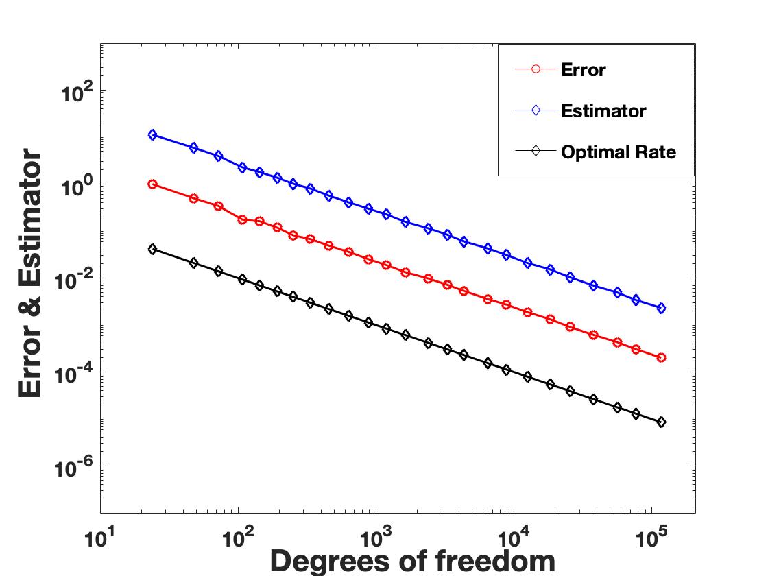
(a) SIPG

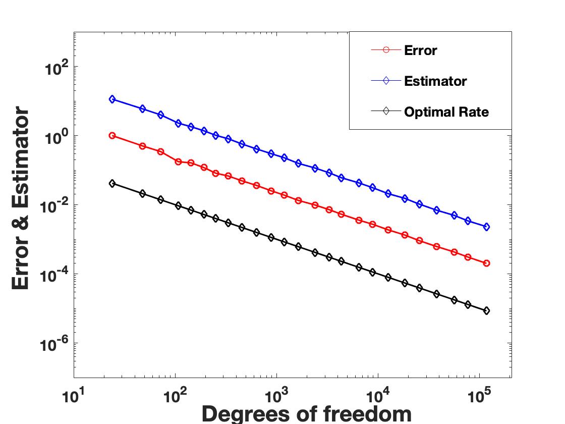
(b) NIPG

Figure 7.1. Convergence of error and estimator for SIPG and NIPG method for Model Problem 1.

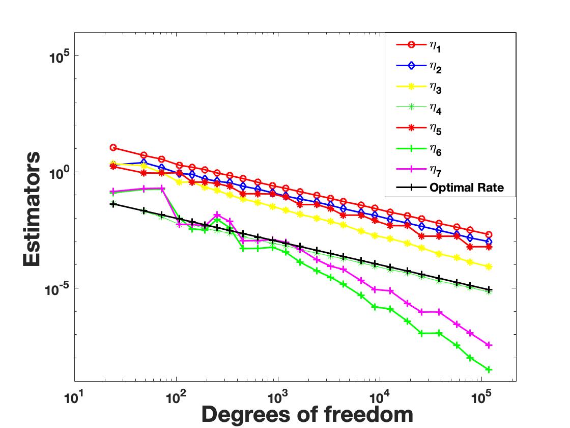
(a) SIPG

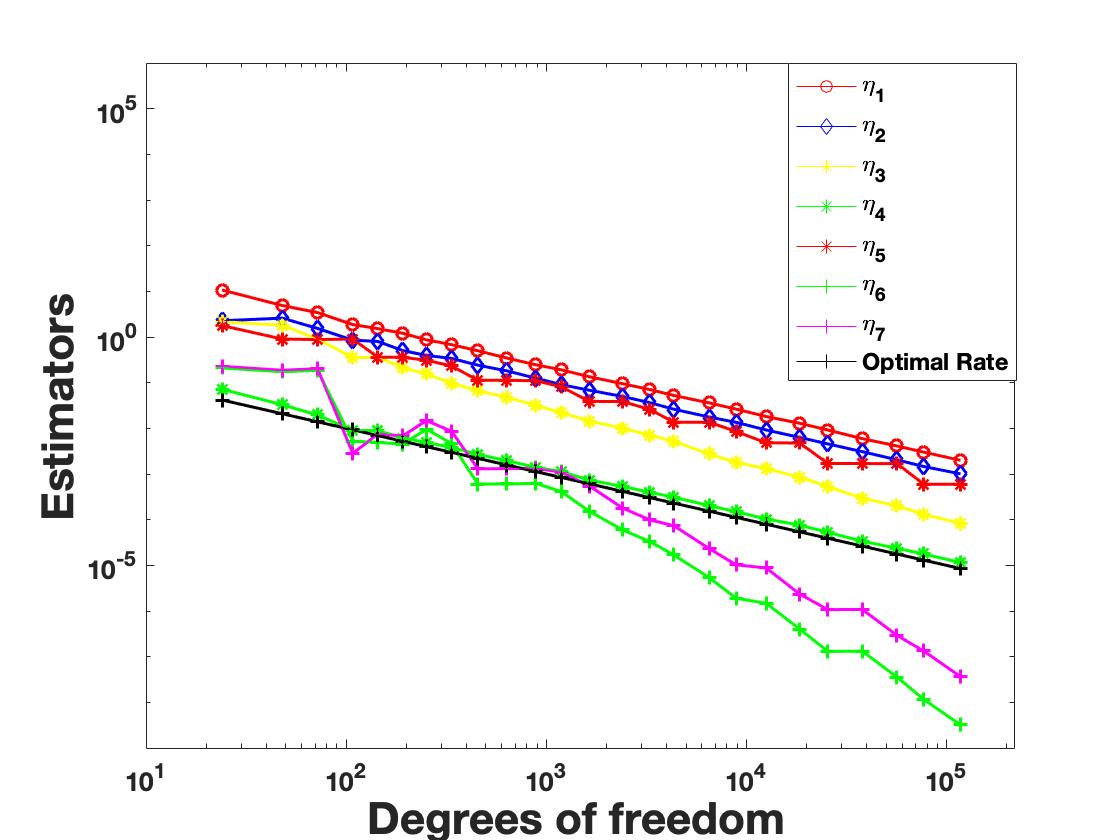
(b) NIPG

Figure 7.2. Error estimator contributions for SIPG and NIPG method for Model Problem 1.

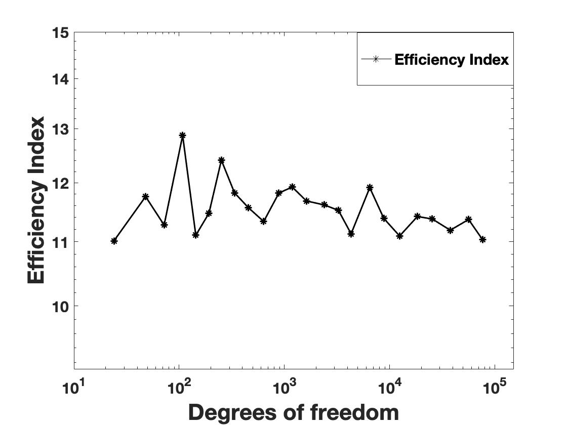
(a) SIPG

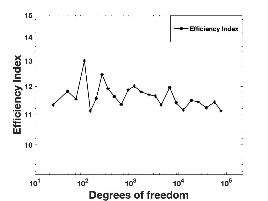
(b) NIPG

Figure 7.3. Plot of efficiency index for SIPG and NIPG method for Model Problem 1.

First, we conduct the numerical test on uniform refined meshes for SIPG and NIPG methods. The smoothness of the exact solution ensures the optimal order of convergence(1/NDof, NDof= Degrees of freedom). Table 7.1 demonstrates the convergence history of energy norm error for SIPG and NIPG methods, respectively on uniform refinement. Next, we conduct the test on adaptive mesh which operates in the following way:

• SOLVE: In this step we compute the solution $\boldsymbol{u_{h}}$ of discrete variational inequality (3.1).

• ESTIMATE: The error estimator $\eta_{h}$ is computed elementwise in this step.

• MARK: We use Dörlfer marking strategy [24] with the parameter $\theta=0.4$ to mark the triangles.

• REFINE: Finally, in this step, we refine the marked triangles using newest vertex bisection algorithm [50] and obtain a finer mesh.

In Figure 7.1, we plot the DG norm error and residual estimator $\eta_{h}$ on the adaptive mesh. Therein, we observe that the error and estimator are converging with the optimal rate with the increase in degrees of freedom, thus ensuring the reliability of the error estimators. Figure 7.2 illustrates the convergence of individual error estimators on the adaptive mesh. The efficiency index which is calculated as ratio of estimator and error is depicted in Figure 7.3. We can see that the graph of efficiency index is both bounded above and below by generic constant which ensures that the residual estimator $\eta_{h}$ is both reliable and efficient.

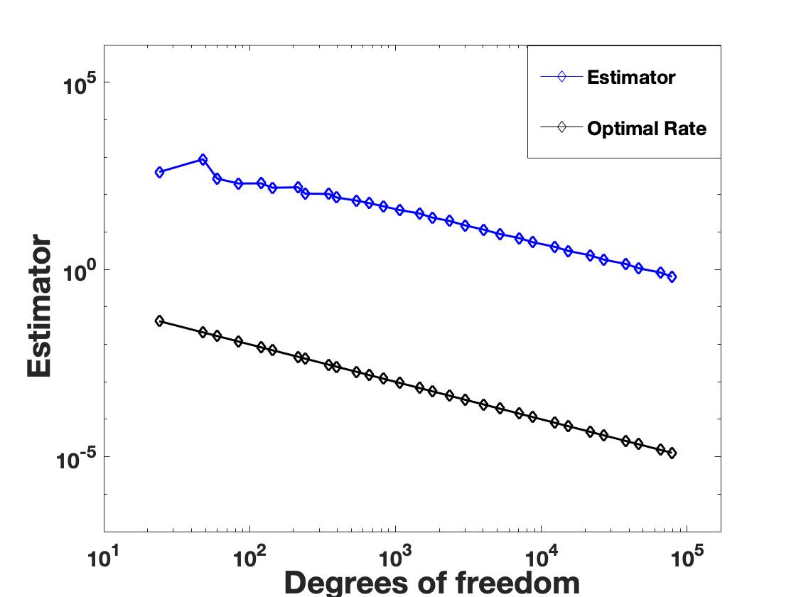
(a) SIPG

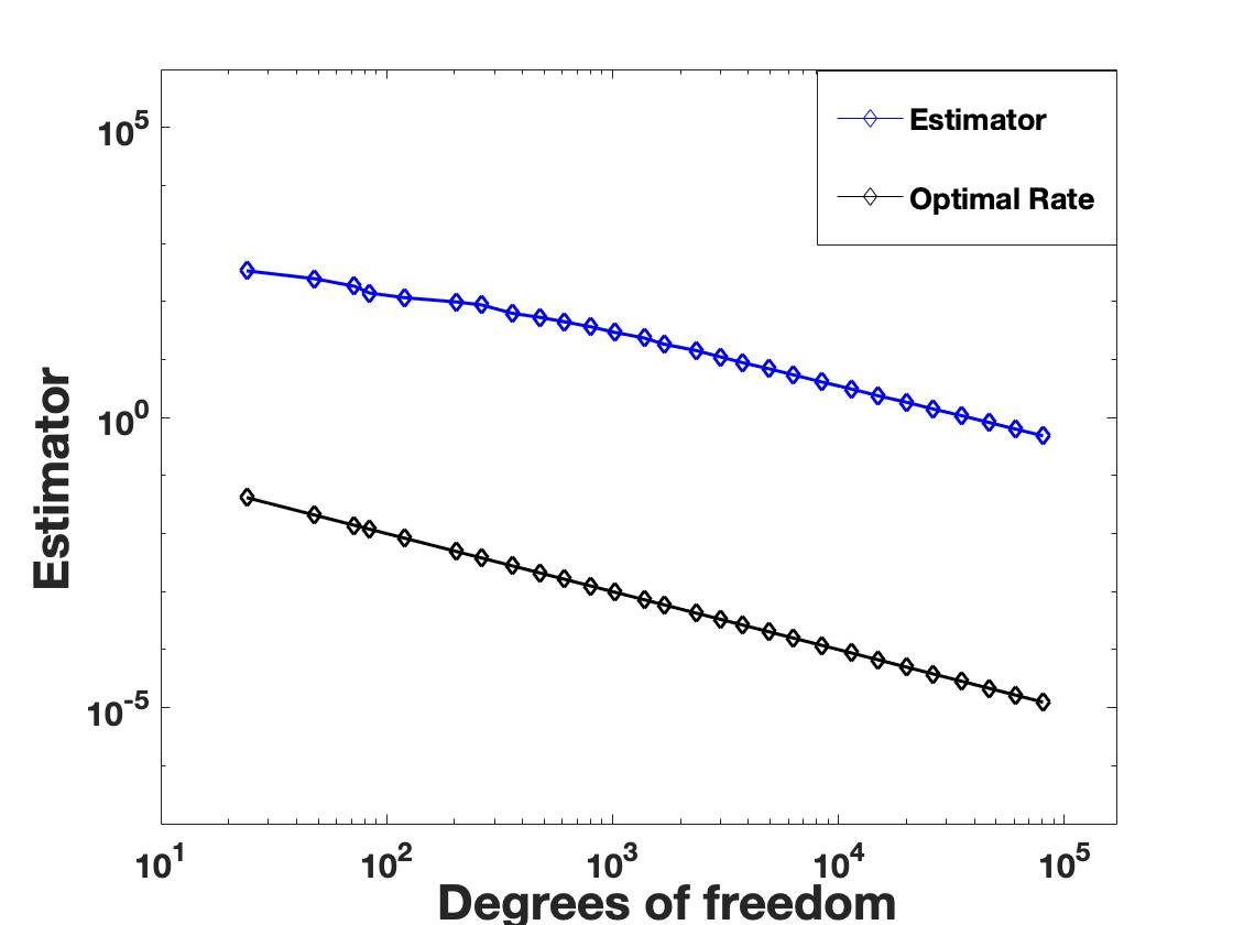
(b) NIPG

Figure 7.4. Convergence of estimator for SIPG and NIPG method for Model Problem 2.

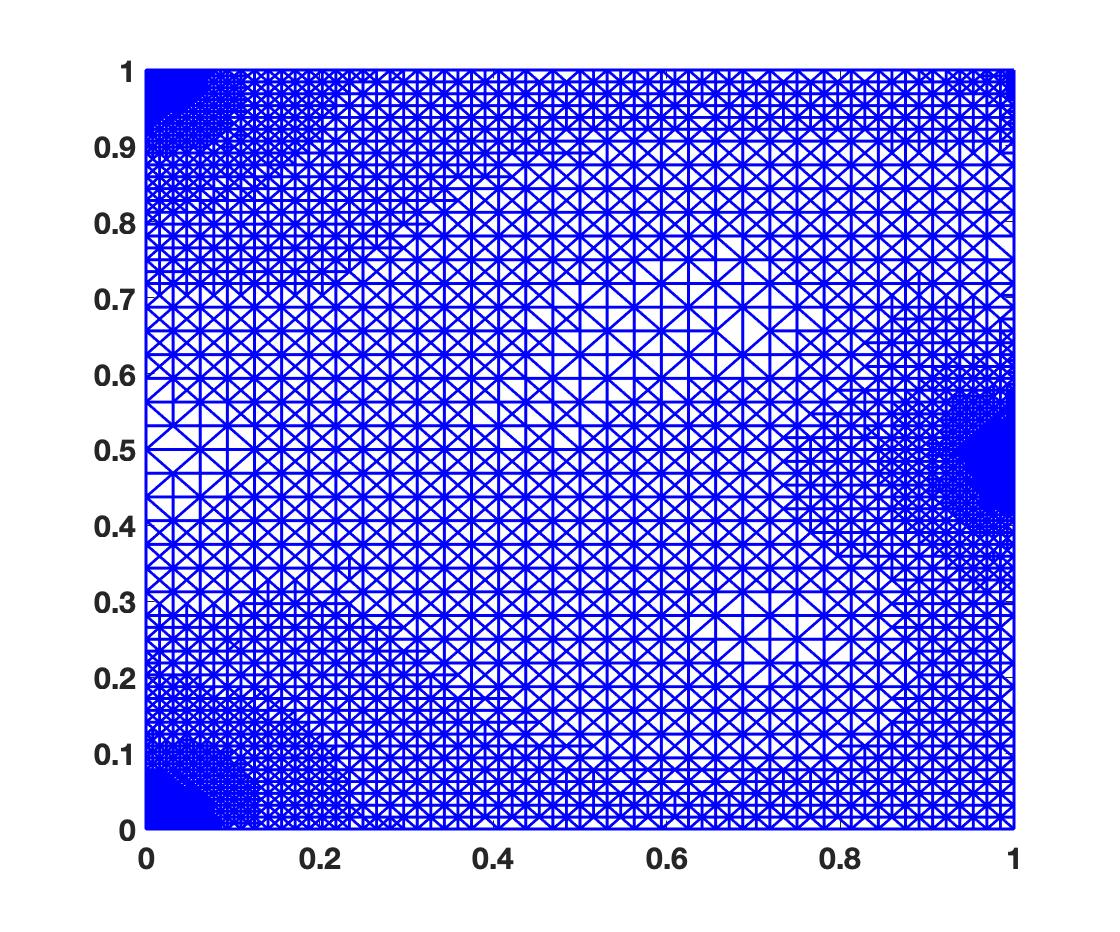
(a) SIPG

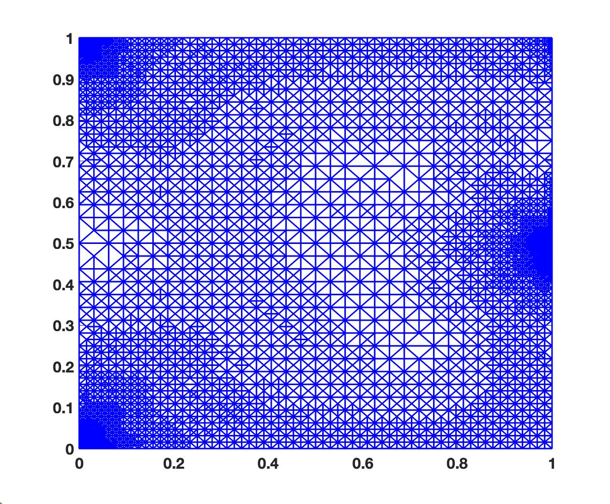
(b) NIPG

Figure 7.5. Adaptive mesh refinement for SIPG and NIPG method for Model Problem 2.

Model Problem 2: (Contact with a rigid wedge)

In the next model problem, the domain $\Omega=(0,1)\times(0,1)$ is the cross section of the linear elastic square which is pushed towards a non-zero obstacle $h(y)=-0.2+\rvert 0.5-y\lvert$ in the direction of potential contact boundary $\{1\}\times(0,1)$ . The Neumann boundary $\big{(}(0,1)\times\{0\}\big{)}\cup\big{(}(0,1)\times\{1\}\big{)}$ is traction free i.e. $\boldsymbol{g}\leavevmode\nobreak\ =\leavevmode\nobreak\ 0$. Next, we impose non-homogeneous Dirichlet boundary condition $\boldsymbol{u}=(-0.1,0)$ on $\{0\}\times(0,1)$. The load vector $\boldsymbol{f}$ is assumed to be zero. The Lam$\acute{e}$ parameters $\mu$ and $\lambda$ are computed by

$$\mu=\frac{E}{2(1+\nu)}\leavevmode\nobreak\ \leavevmode\nobreak\ \text{and}\leavevmode\nobreak\ \leavevmode\nobreak\ \lambda=\frac{E\nu}{(1+\nu)(1-2\nu)},$$

where, the Young’s modulus $E$ and the Poisson ratio $\nu$ are 500 and 0.3, respectively for the given model problem.

In contrast to Model Problem 1, we do not have exact solution for this problem, therefore we only plot the convergence of residual error estimator versus the degrees of freedom. The behaviour of residual error estimator for SIPG and NIPG methods is described in Figure 7.4. Therein, the figure depicts the optimal order of convergence of the estimators. Figure 7.5 illustrates the adaptively refined grid steered by the residual error estimator for both the DG methods. As expected, the mesh is strongly refined near the area where the tip of wedge is coming in the contact with the unit square, free boundary around the contact zone and the intersection of the Neumann and Dirichlet boundaries. Thus, the deformation of the body under the effect of traction is well captured. The decay of individual error estimator $\eta_{i},1\leq i\leq 7$ is plotted in Figure 7.6. It is evident that each estimator contribution is converging with the optimal rate.

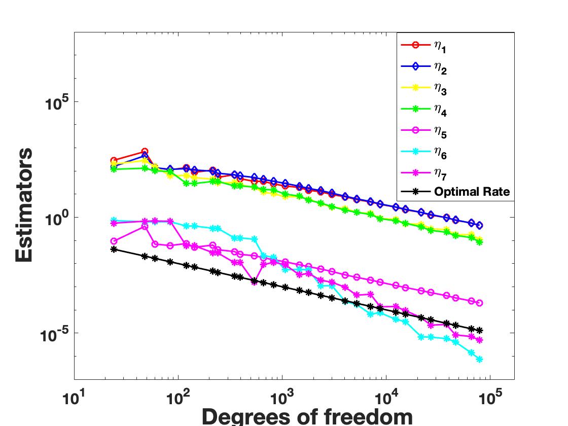
(a) SIPG

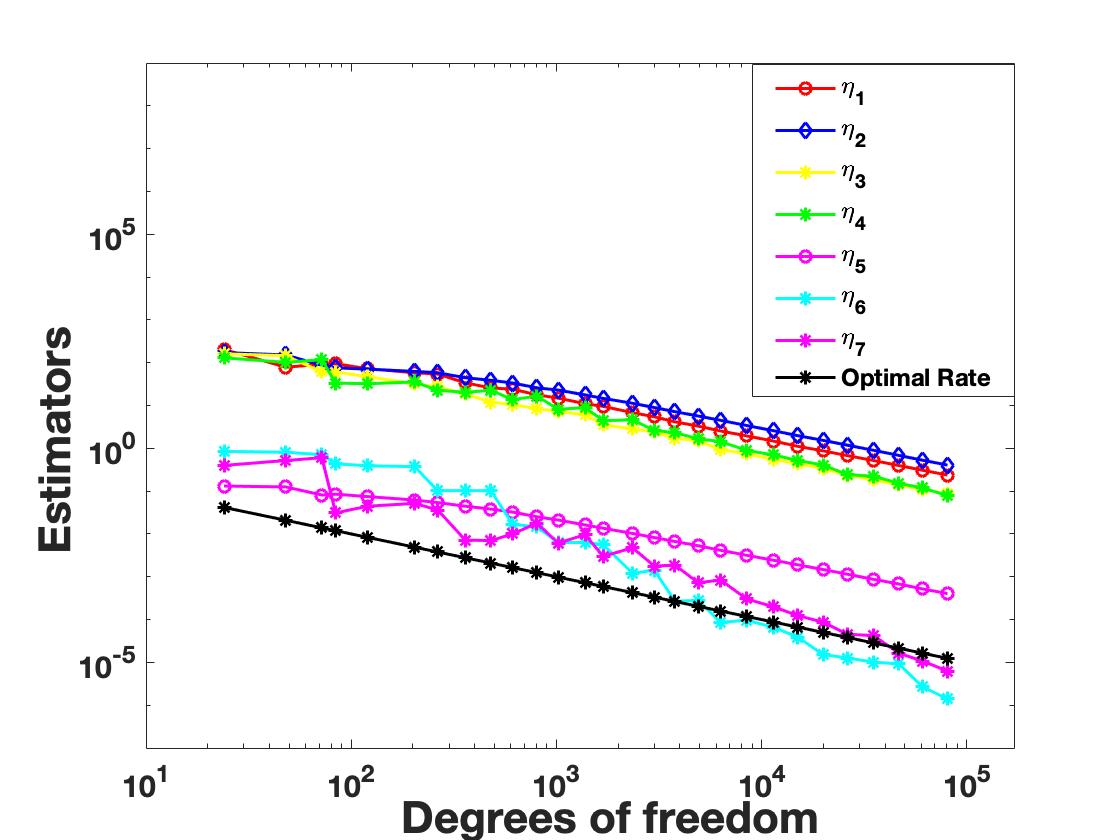
(b) NIPG

Figure 7.6. Residual error estimators contribution for SIPG and NIPG method for Model Problem 2.

References

- [1] M. Ainsworth and J. T. Oden. A posteriori error estimation in finite element analysis. Pure and Applied Mathematics (New York). Wiley-Interscience [John Wiley & Sons], New York, 2000.
- [2] D. N. Arnold. An interior penalty finite element method with discontinuous elements. SIAM J. Numer. Anal., 19:742–760, 1982.
- [3] D. N. Arnold, F. Brezzi, B. Cockburn and L. D. Marini. Unified analysis of discontinuous Galerkin methods for elliptic problems. SIAM J. Numer. Anal., 39:1749–1779, 2002.
- [4] K. Atkinson and W. Han. Theoretical Numerical Analysis. A functional analysis framework. Third edition, Springer, 2009.
- [5] L. Banz and E. P. Stephan. A posteriori error estimates of -adaptive IPDG-FEM for elliptic obstacle problems. Appl. Numer. Math., 76:76–92, 2014.
- [6] L. Banz and A. Schröder. Biorthogonal basis functions in -adaptive FEM for elliptic obstacle problems. Comput. Math. Appl., 70:1721-1742, 2015.
- [7] S. Bartels and C. Carstensen. Averaging techniques yield reliable a posteriori finite element error control for obstacle problems. Numer. Math., 99:225–249, 2004.
- [8] F. Bassi, S. Rebay, G. Mariotti, S. Pedinotti and M. Savini. A high-order accurate discontinuous finite element method for inviscid and viscous turbomachinery flows, in: R. Decuypere, G. Dibelius (Eds.), Proceedings of 2nd European Conference on Turbomachinery, Fluid Dynamics and Thermodynamics, Technologisch Instituut, Antwerpen, Belgium, 99–108, 1997.
- [9] Z. Belhachmi and F. B. Belgacam. Quadratic Finite Element Approximation of the Signorini problem. Math. Comp., 72:83-104, 2001.
- [10] R. E. Bird, W. M. Coombs and S. Giani. A posteriori discontinuous Galerkin error estimator for linear elasticity. Appl. Math. Comp., 344:78–96, 2019.
- [11] V. Bostan and W. Han. A posteriori error analysis for finite element solutions of a frictional contact problem. Comput. Methods Appl. Mech. Engrg., 195:1252–1274, 2006.
- [12] S. C. Brenner. Korn’s inequalities for piecewise vector fields. Math. Comp. 73:1067–1087, 2004.
- [13] S. C. Brenner. Ponicaré-Friedrichs inequalities for piecewise functions. SIAM J. Numer. Anal., 41:306–324, 2003.
- [14] S. C. Brenner, L. Y. Sung and Y. Zhangy. Finite element methods for the displacement obstacle problem of clamped plates. Math. Comp., 81:1247–1262, 2012.
- [15] S. C. Brenner and L. R. Scott. The Mathematical Theory of Finite Element Methods Third Edition. Springer-Verlag, New York, 2008.
- [16] F. Brezzi, W. W. Hager and P. A. Raviart. Error estimates for the finite element solution of variational inequalities, Part I. Primal theory. Numer. Math., 28:431–443, 1977.
- [17] F. Brezzi, G. Manzini, D. Marini, P. Pietra and A. Russo. Discontinuous Galerkin Approximations for elliptic problems. Numer. Met. PDE, 16:365–378, 2000.
- [18] B Rivire, M. F. Wheeler and V. Girault. A priori error estimates for finite element methods based on discontinuous approximation spaces for elliptic problems. SIAM J. Numer. Anal., 39:902-931, 2001.
- [19] R. Bustinza and F. J. Sayas. Error estimates for an LDG method applied to a Signorini type problems. J. Sci. Comput., 52:322–339, 2012.
- [20] P. Castillo, B. Cockburn, I. Perugia and D. Schötzau. An a priori error analysis of the local discontinuous Galerkin method for elliptic problems. SIAM J. Numer. Anal., 38:1676–1706, 2000.
- [21] Y. Chen, J. Huang, X. Huang and Y. Xu. On the local discontinuous Galerkin method for linear elasticity. Math. Probl. Eng., 19:242–256, 2010.
- [22] P. G. Ciarlet. The Finite Element Method for Elliptic Problems. North-Holland, Amsterdam, 1978.
- [23] B. Cockburn, G. E. Karniadakis, C.-W. (eds) Shu. Discontinuous Galerkin Methods. Theory, Computation and Applications, Lecture Notes in Computer Science engineering, Vol. 11, Springer, New York, 2000.
- [24] W. Dörlfer. A convergent adaptive algorithm for Poisson’s equation. SIAM J. Numer. Anal., 33:1106–1124, 1996.
- [25] G. Duvaut and J. L. Lions. Inequalities in Mechanics and Physics. Springer, Berlin, 1976.
- [26] R. S. Falk. Error estimates for the approximation of a class of variational inequalities. Math. Comp., 28:963–971, 1974.
- [27] G. Fichera. Problemi elastostatici con vincoli unilaterali:il problema di signorini con ambigue condizioni al contorno. Mem Accad Naz Lincei Ser, 8:91–140, 1964.
- [28] S. Gaddam and T. Gudi. Bubbles enriched quadratic finite element method for the 3D-elliptic obstacle problem. Comput. Methods Appl. Math., 18:223–236, 2018.
- [29] S. Gaddam, T. Gudi and K. Porwal. Two new approaches for solving elliptic obstacle problems using discontinuous Galerkin methods. BIT Numer. Math., 62:89–124, 2022.
- [30] R. Glowinski. Numerical Methods for Nonlinear Variational Problems. Springer-Verlag, Berlin, 2008.
- [31] T. Gudi and K. Porwal. A remark on the a posteriori error analysis of discontinuous Galerkin methods for obstacle problem. Comput. Meth. Appl. Math., 14:71–87, 2014.
- [32] T. Gudi and K. Porwal. An a posteriori error estimator for a class of discontinuous Galerkin methods for Signorini problem. J. Comp. Appl. Math., 292:257–278, 2016.
- [33] T. Gudi and K. Porwal. A posteriori error control of discontinuous Galerkin methods for elliptic obstacle problems. Math. Comput., 83:579–602, 2014.
- [34] T. Gudi and K. Porwal. A reliable residual based a posteriori error estimator for a quadratic finite element method for the elliptic obstacle problem. Comput. Meth. Appl. Math., 15:145-160, 2014.
- [35] J. S. Hesthaven and T. Warburton. Nodal discontinuous Galerkin methods: Algorithms, Analysis, and Applications, Springer, New York, 2007.
- [36] P. Hild and S. Nicaise. A posteriori error estimations of residual type for Signorini’s problem. Numer. Math., 101:523–549, 2005.
- [37] P. Hild and S. Nicaise. Residual a posteriori error estimators for contact problems in elasticity. ESAIM:M2AN, 41:897–923, 2007.
- [38] S. Hüeber, M. Mair and B. I. Wohlmuth. A priori error estimates and an inexact primal-dual active set strategy for linear and quadratic finite elements applied to multibody contact problems. App. Num. Math., 54:555–576, 2005.
- [39] R. Khandelwal, K. Porwal and T. Wadhawan. Adaptive quadratic finite element method for the unilateral contact problem (Submitted).
- [40] N. Kikuchi and J. T. Oden. Contact Problem in Elasticity. SIAM, Philadelphia, 1988.
- [41] D. Kinderlehrer and G. Stampacchia. An Introduction to Variational Inequalities and Their Applications. SIAM, Philadelphia, 2000.
- [42] R. Krause, A. Veeser and M. Walloth. An efficient and reliable residual-type a posteriori error estimator for the Signorini problem. Num. Math., 130:151–197, 2015.
- [43] R. Nochetto, T. V. Petersdorff and C. S. Zhang. A posteriori error analysis for a class of integral equations and variational inequalities. Numer. Math., 116:519–552, 2010.
- [44] D. Pietro, D. Antonio and A. Ern. Mathematical aspects of discontinuous Galerkin methods. Mathématiques and Appl., Springer, Berlin, 2012.
- [45] W. H. Reed and T. R. Hill. Triangular mesh methods for the neutron transport equation. Technical Report LA-UR-73-479, Los Alamos Scientific Laboratory, 1973.
- [46] B. Rivière. Discontinuous Galerkin Methods for Solving Elliptic and Parabolic Equations: Theory and Implementation, SIAM, Philadelphia, 2008.
- [47] A. Signorini. Questioni di elasticita non-linearizzata e semi-linearizzata. Rendiconti Di Matematica E Delle Sue Applicazioni, 18:95–39, 1959.
- [48] A. Veeser. Efficient and Reliable a posteriori error estimators for elliptic obstacle problems. SIAM J. Numer. Anal., 39:146–167, 2001.
- [49] R. Verfürth. A posteriori error estimation and adaptive mesh-refinement techniques. In Proceedings of the Fifth International Congress on Computational and Applied Mathematics (Leuven, 1992), 50: 67–83, 1994.
- [50] R. Verfürth. A Review of A Posteriori Error Estimation and Adaptive Mesh-Refinement Techniques. Wiley-Teubner, Chichester, 1995.
- [51] M. Walloth. A reliable, efficient and localized error estimator for a discontinuous Galerkin method for the Signorini problem. App. Num. Math., 135:276-296, 2019.
- [52] L. H. Wang. On the quadratic finite element approximation to the obstacle problem. Numer. Math., 92:771-778, 2002.
- [53] F. Wang, W. Han and X. Cheng. Discontinuous Galerkin methods for solving a quasi static contact problem. Numer. Math., 126:771–800, 2014.
- [54] F. Wang, W. Han and X. Cheng. Discontinuous Galerkin methods for solving elliptic variational inequalities. SIAM J. Numer. Anal., 48:708–733, 2010.
- [55] F. Wang, W. Han and X. Cheng. Discontinuous Galerkin methods for solving Signorini problem. IMA J. Numer. Anal., 31:1754–1772, 2011.
- [56] F. Wang, W. Han, J. Eichholz and X. Cheng. A posteriori error estimates for discontinuous Galerkin methods of obstacle problems. Nonlin. Anal. : Real World Appl., 22:664–679, 2015.
- [57] A. Weiss and B. I. Wohlmuth. A posteriori error estimator and error control for contact problems. Math. Comp., 78:1237-1267, 2009.