Radio Map-Based Spectrum Sharing for Joint Communication and Sensing
Abstract
The sixth-generation (6G) network is expected to provide both communication and sensing (C&S) services. However, spectrum scarcity poses a major challenge to the harmonious coexistence of C&S systems. Without effective cooperation, the interference resulting from spectrum sharing impairs the performance of both systems. This paper addresses C&S interference within a distributed network. Different from traditional schemes that require pilot-based high-frequency interactions between C&S systems, we introduce a third party named the radio map to provide the large-scale channel state information (CSI). With large-scale CSI, we optimize the transmit power of C&S systems to maximize the signal-to-interference-plus-noise ratio (SINR) for the radar detection, while meeting the ergodic rate requirement of the interfered user. Given the non-convexity of both the objective and constraint, we employ the techniques of auxiliary-function-based scaling and fraction programming for simplification. Subsequently, we propose an iterative algorithm to solve this problem. Simulation results collaborate our idea that the extrinsic information, i.e., positions and surroundings, is effective to decouple C&S interference.
Index Terms:
Joint communication and sensing (JCAS), large-scale channel state information (CSI), power allocation, radio map, spectrum sharing.I INTRODUCTION
The advent of the fifth-generation (5G) network has ushered in a myriad of applications, ranging from automatic driving and smart manufacturing to telemedicine. These applications not only demand high communication data rates but also require precise sensing. The vision of enabling joint communication and sensing in the sixth-generation (6G) network has become increasingly clear. Driven by the ever-lasting demands, both C&S systems are increasing their scale in the full swing. However, their progress faces a significant obstacle of spectrum scarcity. The interference caused by spectrum sharing impairs the functionalities of both C&S systems [1, 2]. To coexist C&S systems and further build an integrated C&S network, JCAS has become a heated topic in both academia and industry.
In the literature, investigations on JCAS can be classified into two categories [3]. The first is C&S coexistence. In this case, C&S signals are generated and processed by independent C&S hardware. The C&S signals operate in the same frequency band, leading to mutual interference. Related studies mainly focus on the interference management [4, 5]. The second is C&S integration, which aims to integrate C&S functions into a single platform [6, 7]. In C&S integration, corresponding schemes can be further classified into three categories. The first is radar-centric. Related studies take sensing as the primary function and use radars as the dual-function platform [8, 9, 10]. The second is communication-centric. Related studies mainly focus on the data transmission and take the communication transceiver as the dual-function platform [11, 12]. The third category is novel waveform design, which aims to provide flexible C&S services using a new dual-function platform. Studies in this category are actively exploring the fundamental limits of C&S performance in a single transmission. Many dual-function waveforms have been proposed for different scenarios.
Compared with C&S integration, which requires a long-term effort, the severe spectrum scarcity makes C&S coexistence a more urgent task at present. In the literature, many studies have delved into the interference mitigation between wireless communication and radar sensing. In the early stages, related studies were mainly unilateral, making adaptations either on the radar side or the communication side [13]–[22]. On the radar side, Bica et al. used mutual-information-based criteria to optimize the radar waveform [13]. Babaei et al. introduced a null-space precoder that confines radar signals within the null space of interference channels [14]. Shi et al. considered the imperfections of the channel state information (CSI) and proposed a power minimization scheme, with the C&S requirement serving as the constraints [15]. Kang et al. optimized the radar beampattern to manage its radiating energy in spatial directions and spectral frequency bands [16]. Alaee-Kerahroodi et al. proposed a cognitive radar waveform and validated its effectiveness using a custom-built prototype [17]. On the communication side, E. H. G. Yousif et al. devised a linear constraint variance minimization beamforming scheme to control the interference leakage from the base station (BS) to radars [18]. Liu et al. investigated the coexistence between a multi-input and multi-output (MIMO) radar and a multi-user MIMO communication system. They proposed a robust communication precoding scheme to maximize the detection probability while ensuring the minimal signal-to-interference-plus-noise ratio (SINR) of downlink users [19]. Moreover, the authors further paid attention to practical limitations in C&S cooperation [20]. They investigated the channel estimation and radar working mode judgment under different prior knowledge levels of the radar waveform. Wang et al. and Shtaiwi et al. introduced the reconfigurable intelligent surface (RIS) to the C&S network. Both of them investigated the joint BS and RIS precoding scheme to exploit the degrees of freedom (DoFs) of RIS for controlling C&S interference [21, 22].
Due to the limited DoFs, the unilateral schemes are sometimes insufficient to control interference to a required level. The joint C&S cooperation is accepted as a more effective means [23]–[30]. Wang et al. considered a single-antenna C&S network and proposed a joint power allocation scheme from both radar-centric and communication-centric perspectives [23]. Li et al. investigated the matrix-completion-based radars in the coexistence design. With additional DoFs of subsampling of this kind of radar, they established an optimization framework that maximized the radar SINR with the constraint of the communication rate [24]. Qian et al. jointly optimized the radar transmit waveform, receive filter, and code book of the communication system in a clutter environment. To ensure the estimation accuracy, the authors took the waveform similarity as a constraint in the optimization [25]. Given that the interference generated by pulse radars is not constant, Zheng et al. proposed a novel metric named the compound rate to measure the communication performance under varying interference [26]. He et al. proposed a robust coexistence scheme with the objective of minimizing C&S power. The probability that C&S SINRs are below a certain threshold was constrained within a small value [27]. In addition to optimizing the detection performance, Cheng et al. minimized the Cramér-Rao Bound of the angle estimation by optimizing the radar waveform and communication transmit vectors [28]. Grossi et al. maximized the energy efficiency of the communication system while ensuring the received SINR of radars [29]. Qian et al. jointly optimized the radar receiver and communication transmitter to maximize the mutual information between the probing signals and received echoes [30].
Although the studies mentioned above offered valuable insights into mitigating interference between C&S systems, a gap persists between the theoretical investigations and practical deployment. In many cases, practical conditions cannot support the perfect CSI assumption made in the literature. First, obtaining full CSI requires pilot-based channel estimation. It is nearly impossible for existing C&S systems to alter their hardware and software for receiving the counterpart signals. In addition, acquiring full CSI is costly. C&S systems have to send pilots, estimate CSI, and exchange CSI data during each channel coherence time, resulting in heavy signaling overhead. Moreover, C&S systems become less robust using the pilot-based cooperation. Any inaccuracies in CSI degrade cooperation efficiency, impacting the provisions of C&S services. Given these challenges, the pilot-based C&S cooperation may not be a practical choice in real-world applications.
Motivated by the above drawbacks, we propose a radio-map-based C&S cooperation framework. A third party named the radio map is introduced to exploit extrinsic environmental information to estimate the large-scale CSI. By doing so, the pilot-based high-frequency C&S interactions are bypassed. The main contributions of this paper are summarized as follows:
-
1.
We propose a radio-map-based C&S cooperation framework to mitigate C&S interference within a distributed network. Unlike traditional channel estimation relying on pilots, the radio map utilizes extrinsic environmental information to estimate the large-scale CSI. Leveraging this large-scale CSI, we propose a joint power allocation scheme that takes the radar SINR as the objective and the ergodic user rate as the constraint.
-
2.
The formulated problem includes both the non-convex objective and constraint. To tackle the absence of a closed-form expression of the ergodic rate, we construct auxiliary functions and employ the scaling technique. To handle the fractional expression of the radar SINR, we apply the quadratic transformation. Building upon these techniques, we propose an iterative algorithm to solve this problem in low complexity.
-
3.
We employ a learning-based method to construct the radio map and utilize its predicted large-scale CSI to implement the proposed power allocation scheme. Simulation results validate the effectiveness of incorporating extrinsic information to coexist C&S systems in a loose cooperation manner.
The remainder of this paper is organized as follows. In Section II, we introduce the system model and concrete the concept of the radio map. Section III presents the joint power allocation scheme and the iterative algorithm. Section IV introduces simulation results and Section V draws conclusions.
Throughout this paper, vectors and matrices are represented by lower and upper boldface symbols, respectively. represents the set of complex matrices and is the operation of the transpose conjugate. The complex Gaussian distribution of zero mean and variance is denoted as . is the expectation operation with respect to .
II SYSTEM MODEL

In Fig. 1, we illustrate the pilot-based C&S cooperation framework and the proposed radio-map-based C&S cooperation framework. As shown in Fig. 1 (a), the pilot-based C&S cooperation framework requires both signal-level and data-level C&S interactions. Within each channel coherence time, C&S systems exchange pilots, CSI data, and negotiate C&S requirements and allocation results. The two systems are tightly coupled by high-frequency and heavyweight interactions. In contrast, the radio-map-based framework only requires low-frequency and lightweight C&S interactions. Instead of transmitting pilots for CSI acquisition, C&S systems send original data to the radio map and get the large-scale CSI in return. With the radio-map-predicted large-scale CSI, C&S systems only need to negotiate their requirements and resource allocation results. Their negotiation frequency aligns with the varying frequency of the large-scale fading, which changes slowly. In this way, the burden of pilot-based online C&S interactions is alleviated through the offline interactions between the radio map and C&S systems, enabling C&S systems work in a loose cooperation manner.
Based on the proposed framework, we illustrate the specific system model of a radio-map-based distributed C&S network in Fig. 2. The communication system is composed of multiple distributed BSs and the number of BSs is denoted as . These BSs are connected to a common processing center. They serve users in a user centric manner. To avoid inter-user interference, different users are allocated with the orthogonal frequency band. The sensing system is composed of multiple distributed radars and the number of radars is denoted as . These radars operate in the same frequency band and use the orthogonally coded signals to tell from each other. Radars detect a common target. The detection results are sent to the fusion center to calculate the final judgment. In addition to C&S systems, a third party named the radio map is placed in the network. The radio map functions to exploit extrinsic environmental information to estimate the large-scale CSI. To facilitate the negotiation, optical fibers connect the communication processing center, radar fusion center and radio map. In this network, C&S systems share spectrum resources. We concentrate on one user whose allocated frequency band is overlapped with radars. The models and expressions can be extended to the case of multiple interfered users with few changes.
II-A RADIO MAP MODEL
To specify the working regime of the radio-map-based C&S cooperation framework, we detail the inner modules and data flows of these three parties in Fig. 3. As depicted by the yellow blocks, the radio map includes two key modules: data management and radio map estimator. The data management module is responsible for data collection, storage and updates. It collects training data through self-measurement and from C&S systems. In the offline stage, the self-measurement approaches include the ray-tracing-based numerical calculation and on-site measurements. Simultaneously, the historical CSI of C&S systems can be sent to the radio map. In the online stage, the radio map can place dedicated sensors for real-time measurements [31]. Additionally, signals from C&S systems and radar detection results are also valuable real-time data. In each large-scale channel coherence time, the data management module processes the newly collected data and hands over them to the radio map estimator. Leveraging these data, the radio map estimator constructs or updates the estimator. From a mathematical perspective, the estimator is a mapping function, which maps the position data, i.e., the transmitting and receiving (T&R) positions, into the large-scale CSI [32]. In C&S systems, the data management modules collect T&R positions. They send T&R positions to the radio map and get the corresponding large-scale CSI back. In the depicted block diagram, the C&S resource management module resides within the radar fusion center. Consequently, the communication system needs to send its T&R positions to the radar fusion center, enabling the latter to know the large-scale CSI of both systems. With the large-scale CSI, the C&S resource management module runs the built-in algorithm, calculating the resource allocation results. These results are communicated to respective resource management modules and being implemented. It is worth noting that the C&S resource management module can alternatively be positioned within the communication processing center, integrated into the radio map, or function as an independent party to provide interference mitigation services. The specific configuration can be flexibly adapted to practical situations.
To demonstrate the feasibility of the proposed framework, we present a case study of the radio map. A ray tracing software named Wireless Insite was introduced to calculate the large-scale CSI, which is regard as the ground truth data. In Fig. 4 (a), we illustrate the layout set in the software. It is a m m rectangular area, covering the range of . There are randomly distributed buildings and lawns. In this simulation, we equally divided the layout into grids and placed a virtual receiver at each grid point. The software was used to calculate the channel gain between the transmitters (BSs/radars) and virtual receivers. We thereby obtained data points for each BS/radar. Using the data points and the corresponding positions of the virtual receiver, we trained a multi-layer perceptron network for each BS/radar. The network has five hidden layers of dimensions. It takes the receiving position as the input and outputs the channel gain. In Fig. 4 (c), we present the large-scale CSI map estimated by the radio map estimator of BS, . For comparison, the large-scale CSI map generated by Wireless Insite and estimated by the curve fitting method are also presented. The curve fitting method is based on a generic channel model:
where represents the path loss, is the T&R distance, and is the carrier frequency. We applied the least squares method to calculate and using the same training data as the radio map.
Through comparisons, we can see that the radio map provides a more accurate approximation to the real large-scale CSI compared to the curve fitting method. This is because the radio map is environmental-aware. By incorporating T&R positions, the radio map accounts for the losses caused by specific geographical factors of this link. It thus delivers more accurate large-scale CSI than generic empirical models. In addition, the large-scale CSI is quasi-static and slow-varying. For slow-moving scenarios, it is empirically sufficient for the radio map to collect data at the meter-level in the spatial domain and update the estimator at the second-level in the time domain [33]. The C&S interactions are also at the second level. Of course, the specific precision of the radio map and C&S interaction frequency depend on practical situations. Striking a balance between overhead and accuracy is crucial for ensuring the practical viability and effectiveness of the radio-map-based framework.
II-B CHANNEL MODEL
In this subsection, we introduce the channel model. We assume that BSs and radars are equipped with a single antenna. This is because, in MIMO systems, the precoding scheme that exploits the multiplexing gain requires perfect and instantaneous CSI [34]. With only large-scale CSI available, multiple antennas are equivalent to a combined single antenna for both BSs and radars. The interfered user is assumed to have antennas, which is used to receive different signals from distributed BSs. On this basis, we denote the BS-user link and interference links, i.e., BS-radar link and radar-user link as , , and , respectively, where denotes the index number of radars. They are modeled by the composite channel model:
| (1) | ||||
where , , and denote the large-scale fading. and are diagonal matrices whose th diagonal elements are denoted as and . , , and denote the small-scale fading, whose elements are uniformly and independently conformed to the Gaussian distribution, i.e., . For the two-way links between the radars and target, i.e., , they are modeled by the determined channel model. This is because, in the case of surveillance radars, the detected target is more likely to be in the sky. The corresponding air-to-ground channel is dominated by the line-of-sight path with little random fading.
II-C SIGNAL MODEL
As for the sensing system, radars use orthogonally-coded signals and independently detect a mutual target. Assuming that the delay and Doppler shift are perfectly compensated, the received echo of radar is given by
| (2) |
where and denote the transmit signals of radars and BSs, and is the additive white Gaussian noise. To distinguish the echo of radar from that of others, the radar receiver is equipped with a matched filter (MF), i.e., :
| (3) |
where is the transmit power of radar . After going through the MF and being sampled by the analog-to-digital converter, the expression of the discrete echo is given by [23]
| (4) | ||||
where is the discrete time index and is the sampling number in a coherent processing interval (CPI). For the sake of convenient expression, we omit the index in the following expression. is the th element of , which is rightly the two-way link between radar and the target. is the transmit power matrix of BSs. Similarly, we denote the transmit power matrix of radars as . is the additive white Gaussian noise, which conforms to the distribution and is the MF output of communication signals, which conforms to the distribution. Based on (4), we calculate the received SINR of radar , which is a function of the transmit power of BSs and radars, i.e., :
| (5) | ||||
where denotes the interference-plus-noise suffered by radar . The radar uses the generalized likelihood ratio test to judge the presence of the target. The detection probability and false alarm probability, denoted as and , are calculated as follows [15],
| (6) |
where is the detection threshold determined by the false alarm probability. Given the requirement of the false alarm probability, is a function of the radar SINR. Therefore, we take the radar SINR as the sensing metric.
In terms of the communication system, the received signal of the interfered user is given by
| (7) |
where and are the transmit signals of BSs and radars, and is the white noise that conforms to the distribution. Given the large-scale CSI, the ergodic rate of the interfered user, denoted as , can be calculated:
| (8) |
where
| (9) |
which denotes the interference-plus-noise suffered by the user.
III LARGE-SCALE-CSI-BASED POWER ALLOCATION
III-A PROBLEM FORMULATION
Leveraging the large-scale CSI, we take the minimal received SINR of radars as the objective and the ergodic rate requirement of the interfered user as the constraint. Given the maximal transmit power of BSs and radars, denoted as and , and the power budgets of C&S systems, denoted as and , the joint power allocation problem is formulated as follows:
| (10a) | ||||
| (10b) | ||||
| (10c) | ||||
| (10d) | ||||
| (10e) | ||||
| (10f) | ||||
where (10b) is the ergodic rate requirement of the communication user, (10c) and (10d) are the maximal transmit power constraints of BSs and radars, and (10e) and (10f) are the sum-power constraints of C&S systems.
III-B ITERATIVE ALGORITHM
III-B1 CLOSED-FORM APPROXIMATION
(P1) is highly complex due to the non-convexity of the objective and constraint. The most challenging aspect is the ergodic rate expression (8), which is encapsulated within the expectation operation and lacks a closed-form representation. To address this challenge, we first introduce a determined approximation to [35]:
| (11) | |||
where is determined by the following fixed-point equation,
| (12) |
The aforementioned approximation is derived under the assumption that transmitters and receivers are equipped with an infinite number of antennas. In this limit, the random channel matrix tends to be deterministic. Leveraging the random matrix theory, we can extract the expectation operation and derive this approximation. Readers can refer to [35] for a detailed proof. On this basis, we transform (P1) into the following problem,
| (13a) | ||||
| (13b) | ||||
| (13c) | ||||
| (13d) | ||||
| (13e) | ||||
| (13f) | ||||
| (13g) | ||||
However, remains a complex expression. It includes a fixed point , which is determined by the nonlinear equality (13c). To address this challenge, we apply auxiliary functions and scaling techniques, as detailed in the next subsection.
III-B2 AUXILIARY-FUNCTION-BASED SCALING
We use the right side of (12) to replace the term in (11). This introduces an auxiliary function, denoted as :
| (14) | ||||
Obviously, when , has the following connection with the ergodic rate expression:
| (15) |
In addition, we propose the following Lemma.
Lemma:
On the condition of , the following equation holds:
| (16) |
proof 1:
See Appendix A.
Based on the lemma, the ergodic rate constraint (13b) can be converted into a less-than-max inequality and further scaled into
| (17) | ||||
On this basis, we rewrite (P2) as
| (18a) | ||||
| (18b) | ||||
| (18c) | ||||
| (18d) | ||||
| (18e) | ||||
| (18f) | ||||
| (18g) | ||||
| (18h) | ||||
Moving forward, we reorganize as
| (19) | ||||
Through observations, it is easy to find that the fraction term, i.e., , occurs twice in . Motivated by this, we introduce a group of variables, denoted as , to replace these fraction terms. Then, we transfer the auxiliary function into :
| (20) |
Correspondingly, we denote and is given by
| (21) |
Similar to (15), when and , we have
| (22) |
Since and are monotonically increasing with , it is easy to find that is an increasing function of and . Therefore, we have the following equation,
| (23) |
On this basis, the ergodic rate constraint can be further scaled into
| (24) | ||||
Based on (24), we rewrite (P3) into (P4)
| (25a) | ||||
| (25b) | ||||
| (25c) | ||||
| (25d) | ||||
| (25e) | ||||
| (25f) | ||||
| (25g) | ||||
| (25h) | ||||
| (25i) | ||||
To further simplify this problem, we rewrite the fixed-point equation (12) as follows:
| (26) |
Since is monotonically decreasing with , is equivalent to
| (27) |
which can be further simplified as
For , the logarithmic operation is applied to simplify this constraint,
| (28) | ||||
On this basis, we transform (P4) into (P5)
| (29a) | ||||
| (29b) | ||||
| (29c) | ||||
| (29d) | ||||
| (29e) | ||||
| (29f) | ||||
| (29g) | ||||
| (29h) | ||||
| (29i) | ||||
| (29j) | ||||
Moving forward, we address the non-convex objective. This max-min optimization can be equivalently rewritten as
| (30a) | ||||
| s.t. | (30b) | |||
where is an introduced auxiliary variable. Since is a ratio expression of and , (30b) can be tackled by the fraction programming scheme named quadratic transform [36],
| (31) |
where is an auxiliary variable. The solution to (31), denoted as , can be calculated by a closed-form expression,
| (32) |
| (33) |
| (34) | ||||
On this basis, we propose our iterative algorithm. Taking iteration as an example, we calculate according to (32) using the transmit power obtained in iteration , i.e., and . Then, we use it to replace in the iteration and (31) is simplified as
| (35) |
As for constraints (29b), (29c) and (29d), the Taylor expansion is used to linearize the non-convex terms therein. On this basis, (P5) is transformed into a series of iterative convex problems. The problem in iteration is given by
| (P6) | (36a) | |||
| (36b) | ||||
| (36c) | ||||
| (36d) | ||||
| (36e) | ||||
| (36f) | ||||
| (36g) | ||||
| (36h) | ||||
| (36i) | ||||
| (36j) | ||||
| (36k) | ||||
where and are the Taylor expansion expressions of and . Their expressions are given at the top of the this page. The detailed algorithm is summarized in Algorithm 1. The proof of convergence is given in Appendix B.
IV SIMULATION RESULTS AND DISCUSSIONS
In this section, we present simulation results and discussions. The simulation layout is the same as that we established in the case study of the radio map, as presented in Fig. 4 (a). The layout includes three BSs, i.e., , two radars, i.e., , one interfered user, and a red diamond-shaped target. They are located at (604 m, 629 m), (1289 m, 2022 m), (1986 m, 1316 m), (-1167 m, 3125 m), (2620 m, -779 m), (650 m, 1134 m), and (1360 m, 1000 m), respectively. BSs and the interfered user are equipped with half-wave dipole antennas. The antenna number of the user is equal to the number of BSs, i.e, . Radars are equipped with directional antennas. The maximum antenna gain is dBi and the half-power beam width, denoted as , is . The carrier frequency is GHz, which is the frequency band of the surveillance radar, and the noise variance is [32]. Power related parameters are set as W, W, kW and kW. This is because radars have much higher power than BSs [24]. The sampling number of radars is per CPI, the false alarm probability is , and thus, according to (6).
We first evaluate the impact of large-scale CSI accuracy on C&S performance. As shown in Fig. 5, the curve corresponding to the radio-map-predicted large-scale CSI closely aligns with the one using the real data, while the curve obtained through the curve-fitting method exhibits a noticeable gap. This discrepancy is expected, given that the radio map provides a more accurate estimation of the real data, as demonstrated in Fig. 4. In our case study, the average deviations of the large-scale CSI map generated by the radio map are below dB while the deviations associated with the curve-fitting method exceed dB. Such a substantial deviation leads to misinformed power allocation and, consequently, significant performance deterioration. Therefore, compared with the generic channel model, which is blind to the surrounding environment, the radio map verifies the importance of being environmental-aware. In addition, since the radio map does not require the pilot-based C&S interactions, it is cost-effective for practical applications.
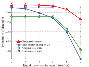
In Fig. 6, we compare the proposed scheme with the scheme proposed in [23] and the unilateral schemes of optimizing or only. Since the scheme proposed in [23] considered the power allocation between one BS and one radar, we used the equal power allocation among different BSs and radars for a fair comparison. The equal power allocation was also used on the not optimized side in the simulation of the unilateral schemes. The results demonstrate that, under the same ergodic rate requirement, the proposed scheme achieves the highest detection probability. Leveraging the large-scale CSI, the proposed scheme intelligently allocates more power to the BSs and radars with favorable serving channels and unfavorable interference channels. This amplifies the positive effects of power for their own systems while constraining the negative effects on the opposite system. As a result, the interference between C&S systems is significantly decoupled in the spatial domain. In contrast, the scheme proposed in [23] is blind to the large-scale CSI, treating all BSs and radars equally in the power allocation. This uniform allocation can not avoid signal collisions, especially when the transmitting equipment on one side and the receiving equipment on the other side are in close proximity. As for unilateral schemes, their efficacy is constrained by the limited DoFs. Only optimizing even failed to provide solutions when bits/s/Hz in the considered setting. The is because when the sensing system does not cooperate to control its power, the interfered user is exposed to a strong-interference environment. Under the given power constraints, the ergodic user rate is limited to below bits/s/Hz, regardless of how the communication power is allocated. In this sense, the joint power allocation is more effective to provide scalable C&S services.
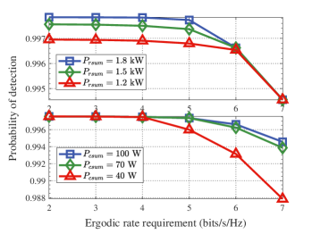
In Fig. 7, we show the impact of the power budgets, i.e., and , on C&S performance. It is evident that the detection performance improves with the availability of the power budgets. In addition, we find that the curves under different overlap when the ergodic rate requirement of the interfered user, i.e., , is low, and the curves under different overlap when is high. The reason is that, when is low, the communication side can meet the ergodic rate requirement without utilizing its full power. To maximize the radar SINR, the communication side conservatively reserves power and the sensing side operates at full capacity. Consequently, the curves under different overlap. In contrast, when is high, the sensing side has to control its power and the communication side works at full capacity. This leads to the curves of different overlapping in the high region. We further find that, in spectrum sharing scenarios where two systems are mutually restricted, the optimal solution lies at the boundary of the feasible set but not within it. In other words, one system must exhaust its resources in the optimal solution.
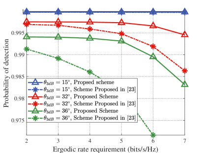
In Fig. 8, we show the impact of radar antenna directivity, depicted by the half-power beam width, i.e., , on the system performance. It can be seen that the detection probability experiences serve degradation as the half-power beam width increases. This is because the larger beam width leads to more power leakage to the communication user and also opens a larger hole to receive BS interference. In addition, the results show that the gap between the proposed scheme and the scheme proposed in [23] is more obvious when is large. The reason is that, when is small, the C&S signals are largely decoupled by directional beams. The improved space left for the proposed scheme is restricted [23]. In contrast, when is large, C&S signals are mutually coupled. The proposed scheme functions like directive beams to separate C&S signals into a comb-like pattern. Consequently, it significantly outperforms the scheme proposed in [23]. This reveals that the proposed large-scale-CSI-based scheme works in the spatial domain, essentially optimizing the spatial distribution of power to mitigate C&S interference.
V CONCLUSIONS
In this paper, we have addressed C&S interference within a distributed network. Given that the available C&S cooperation is limited in the real world, we have proposed a radio-map-based C&S cooperation framework. The radio map has been used to estimate the large-scale CSI so that the pilot-based C&S interactions are bypassed. With the large-scale CSI, we have devised a joint power allocation scheme to maximize the radar detection performance while ensuring the ergodic rate requirement. To handle the non-convex C&S metrics, we have employed the techniques of auxiliary-function-based scaling and fractional programming. The proposed problem has been effectively solved using an iterative algorithm. Simulation results have verified that the extrinsic information, i.e., positions and surroundings, is effective to coordinate conflicting signals in the spatial domain. The proposed scheme provides a viable solution for the coexistence of C&S systems in a loose cooperation manner.
Appendix A PROOF OF LEMMA
We calculate the derivative of ,
Therefore, under the condition of , is monotonically increasing with . Since we have when , it is obvious that the Lemma holds if is monotonically increasing with .
Appendix B PROOF OF CONVERGENCE OF THE ITERATIVE ALGORITHM
For the convenience of expression, we introduce a function to represent the left side of (31):
Therefore, the objective of the proposed iterative algorithm can be rewritten as
| (37) |
Define as the optimal solution obtained in iteration . Then, we have that
| (38) | ||||
In addition, since is the optimal solution to , we can derive the following inequalities:
| (39) | ||||
Combining (38) and (39), it is easy to conclude that the value of the objective is at least not decreasing in the iterative process:
| (40) | ||||
According to the monotonous boundary theorem, the proposed iterative algorithm is assured to be convergent.
References
- [1] Z. Feng, Z. Fang, Z. Wei, X. Chen, Z. Quan, and D. Ji, “Joint radar and communication: A survey,” China Commun., vol. 17, no. 1, pp. 1-27, Jan. 2020.
- [2] J. A. Zhang, F. Liu, C. Masouros et al., “An overview of signal processing techniques for joint communication and radar sensing,” IEEE J. Sel. Top. Signal Process., vol. 15, no. 6, pp. 1295-1315, Nov. 2021.
- [3] X. Fang, W. Feng, Y. Chen, N. Ge, and Y. Zhang, “Joint communication and sensing toward 6G: Models and potential of using MIMO,” IEEE Internet Things J., vol. 10, no. 5, pp. 4093-4116, Mar. 2023.
- [4] S. K. Agrawal, A. Samant, and S. K. Yadav, “Spectrum sensing in cognitive radio networks and metacognition for dynamic spectrum sharing between radar and communication system: A review,” Phys. Commun., vol. 52, Jun. 2022.
- [5] H. T. Hayvaci and B. Tavli, “Spectrum sharing in radar and wireless communication systems: A review,” in Proc. 2014 Int. Conf. Electron. Adv. Appl. (ICEAA), Palm Beach, Aruba, 2014, pp. 810-813.
- [6] F. Liu, Y. Cui, C. Mascouros, J. Xu et al., “Integrated sensing and communications: Toward dual-functional wireless networks for 6G and beyond,” IEEE J. Sel. Areas Commun., vol. 40, no. 6, pp. 1728-1767, Jun. 2022.
- [7] A. Liu, Z. Huang, M. Li et al., “A Survey on fundamental limits of integrated sensing and communication,” IEEE Commun. Surv. Tutorials, vol. 24, no. 2, pp. 994-1034, Q2nd 2022.
- [8] A. Hassanien, M. G. Amin, Y. D. Zhang, and F. Ahmad, “Dual-function radar-communications: Information embedding using sidelobe control and waveform diversity,” IEEE Trans. Signal Process., vol. 64, no. 8, pp. 2168-2181, Apr. 2016.
- [9] A. Hassanien, M. G. Amin, Y. D. Zhang, and F. Ahmad, “Signaling strategies for dual-function radar communications: An overview,” IEEE Aerosp. Electron. Syst. Mag., vol. 31, no. 10, pp. 36-45, Oct. 2016.
- [10] A. Hassanien, M. G. Amin, E. Aboutanios and B. Himed, “Dual-function radar communication systems: A solution to the spectrum congestion problem,” IEEE Signal Process. Mag., vol. 36, no. 5, pp. 115-126, Sep. 2019.
- [11] J. A. Zhang, Md. L. Rahman, K. Wu et al., “Enabling joint communication and radar sensing in mobile networks—A survey,” IEEE Commun. Surv. Tutorials, vol. 24, no. 1, pp. 306-345, Q1th 2022.
- [12] A. Zhang, M. L. Rahman, X. Huang, Y. J. Guo, S. Chen, and R. W. Heath, “Perceptive mobile networks: Cellular networks with radio vision via joint communication and radar sensing,” IEEE Veh. Technol. Mag., vol. 16, no. 2, pp. 20-30, Jun. 2021.
- [13] M. Bica, K. W. Huang, V. Koivunen, and U. Mitra, “Mutual information based radar waveform design for joint radar and cellular communication systems,” in Proc. IEEE Int. Conf. Acoust., Speech Signal Process.(ICASSP), Shanghai, China, Mar. 2016, pp. 3671-3675.
- [14] A. Babaei, W. H. Tranter, and T. Bose, “A nullspace-based precoder with subspace expansion for radar/communications coexistence,” in Proc. 2013 IEEE Global Commun. Conf. (GLOBECOM), Atlanta, GA, USA, 2013, pp. 3487-3492.
- [15] C. Shi, F. Wang, M. Sellathurai, J. Zhou, and S. Salous, “Power minimization-based robust OFDM radar waveform design for radar and communication systems in coexistence,” IEEE Trans. Signal Process., vol. 66, no. 5, pp. 1316-1330, Mar. 2018.
- [16] B. Kang, O. Aldayel, V. Monga, and M. Rangaswamy, “Spatio-spectral radar beampattern design for coexistence with wireless communication systems,” IEEE Trans. Aerosp. Electron. Syst., vol. 55, no. 2, pp. 644-657, Apr. 2019.
- [17] M. Alaee-Kerahroodi, E. Raei, S. Kumar, and B. S. M. R. R., “Cognitive radar waveform design and prototype for coexistence with communications,” IEEE Sens. J., vol. 22, no. 10, pp. 9787-9802, May 2022.
- [18] E. H. G. Yousif, M. C. Filippou, F. Khan, T. Ratnarajah, and M. Sellathurai, “A new LSA-based approach for spectral coexistence of MIMO radar and wireless communication systems,” in Proc. 2016 IEEE Intern. Conf. Commun. (ICC), Kuala Lumpur, Malaysia, 2016, pp. 1-6.
- [19] F. Liu, C. Masouros, A. Li, and T. Ratnarajah, “Robust MIMO beamforming for cellular and radar coexistence,” IEEE Wireless Commun. Lett., vol. 6, no. 3, pp. 374-377, Jun. 2017.
- [20] F. Liu, A. Garcia-Rodriguez, C. Masouros, and G. Geraci, “Interfering channel estimation in radar-cellular coexistence: How much information do we need?,” IEEE Trans. Wireless Commun., vol. 18, no. 9, pp. 4238-4253, Sep. 2019.
- [21] X. Wang, Z. Fei, J. Guo, Z. Zheng, and B. Li, “RIS-assisted spectrum sharing between MIMO radar and MU-MISO communication systems,” IEEE Wireless Commun. Lett., vol. 10, no. 3, pp. 594-598, Mar. 2021.
- [22] E. Shtaiwi, H. Zhang, A. Abdelhadi, and Z. Han, “Sum-rate maximization for RIS-assisted radar and communication coexistence system,” in Proc. 2021 IEEE Global Commun. Conf. (GLOBECOM), 2021, pp. 01-06.
- [23] F. Wang and H. Li, “Joint power allocation for radar and communication co-existence,” IEEE Signal Process. Lett., vol. 26, no. 11, pp. 1608-1612, Nov. 2019.
- [24] B. Li and A. P. Petropulu, “Joint transmit designs for coexistence of MIMO wireless communications and sparse sensing radars in clutter,” IEEE Trans. Aerosp. Electron. Syst., vol. 53, no. 6, pp. 2846-2864, Dec. 2017.
- [25] J. Qian, M. Lops, L. Zheng, X. Wang, and Z. He, “Joint system design for coexistence of MIMO radar and MIMO communication,” IEEE Trans. Signal Process., vol. 66, no. 13, pp. 3504-3519, Jul. 2018.
- [26] L. Zheng, M. Lops, X. Wang, and E. Grossi, “Joint design of overlaid communication systems and pulsed radars,” IEEE Trans. Signal Process., vol. 66, no. 1, pp. 139-154, Jan. 2018.
- [27] X. He and L. Huang, “Robust coexistence design of MIMO radar and MIMO communication under model uncertainty,” in Proc. 2020 IEEE 11th Sens. Array Multichannel Signal Process. Workshop (SAM), 2020, pp. 1-5.
- [28] Z. Cheng, B. Liao, S. Shi, Z. He, and J. Li, “Co-Design for overlaid MIMO radar and downlink MISO communication systems via Cramér-Rao bound minimization,” IEEE Trans. Signal Process., vol. 67, no. 24, pp. 6227-6240, Dec. 2019.
- [29] E. Grossi, M. Lops, and L. Venturino, “Energy efficiency optimization in radar-communication spectrum sharing,” IEEE Trans. Signal Process., vol. 69, pp. 3541-3554, 2021.
- [30] J. Qian, S. Wang, Z. Chen, G. Qian, and N. Fu, “Robust design for spectral sharing system based on MI maximization under direction mismatch,” IEEE Trans Veh. Technol., vol. 71, no. 6, pp. 6831-6836, Jun. 2022.
- [31] S. Bi, J. Lyu, Z. Ding, and R. Zhang, “Engineering radio maps for wireless resource management,” IEEE Wireless Commun., vol. 26, no. 2, pp. 133-141, Apr. 2019.
- [32] W. Feng et al., “Radio map-based cognitive satellite-UAV networks towards 6G on-demand coverage,” IEEE Trans. Cognit. Commun. Netw., Early Access, Dec. 2023.
- [33] Y. Zeng and X. Xu, “Toward environment-aware 6G communications via channel knowledge map,” IEEE Wireless Commun., vol. 28, no. 3, pp. 84-91, Jun. 2021.
- [34] D. P. Palomar, J. M. Cioffi, and M. A. Lagunas, “Joint Tx–Rx beamforming design for multicarrier MIMO channels: A unified framework for convex optimization,” IEEE Trans. Signal Process., vol. 51, no. 9, pp. 2381-2401, Sep. 2003.
- [35] W. Feng, Y. Wang, N. Ge, J. Lu, and J. Zhang, “Virtual MIMO in multi-cell distributed antenna systems: Coordinated transmissions with large-scale CSIT,” IEEE J. Sel. Areas Commun,, vol. 31, no. 10, pp. 2067-2081, Oct. 2013.
- [36] K. Shen and W. Yu, “Fractional programming for communication systems—part I: Power control and beamforming,” IEEE Trans. Signal Process., vol. 66, no. 10, pp. 2616-2630, May 2018.