Chebyshev Subdivision and Reduction Methods for Solving Multivariable Systems of Equations

Abstract.

We present a new algorithm for finding isolated zeros of a system of real-valued functions in a bounded interval $I$ in $\mathbb{R}^{n}$. It uses the Chebyshev proxy method combined with a mixture of subdivision, reduction methods, and elimination checks that leverage special properties of Chebyshev polynomials. We prove the method has R-quadratic convergence locally near simple zeros of the system. We also analyze the temporal complexity and the numerical stability of the algorithm and provide numerical evidence in dimensions up to three that the method is both fast and accurate on a wide range of problems. The algorithm should also work well in higher dimensions. Our tests show that the algorithm outperforms other standard methods on this problem of finding all real zeros in a bounded domain. Our Python implementation of the algorithm is publicly available at https://github.com/tylerjarvis/RootFinding.

1. Introduction

This paper presents a new algorithm for finding isolated zeros of a system of functions $f_{1},\dots,f_{n}$ in a compact interval $I$ of the form $I=[a_{1},b_{1}]\times\cdots\times[a_{n},b_{n}]\subset\mathbb{R}^{n}$. Assuming the functions $f_{1},\dots,f_{n}$ are sufficiently smooth, they can be closely approximated by Chebyshev polynomials $p_{1},\dots,p_{n}$, and this approximation can be done rapidly using the FFT.

Our particular implementation requires that the functions $f_{1},\dots,f_{n}$ are real-analytic on the interval $I$, which implies that the approximations converge geometrically. This allows us, with a little more numerical work, to construct a bound $\varepsilon_{k}$ on the maximum approximation error $\max_{{{{\mathbf{x}}}}\in I}|p_{k}({{{\mathbf{x}}}})-f_{k}({{{\mathbf{x}}}})|\leq\varepsilon_{k}$ over the interval $I$ for all $k\in\{1,\dots,n\}$. If the functions are not analytic, one could still construct an error approximation that accounts for the correspondingly slower rate of convergence

The approximations $p_{1},\dots,p_{n}$, and error bounds $\varepsilon_{1},\dots,\varepsilon_{n}$, transform the problem into that of finding small subintervals of $I$ where every polynomial $p_{k}$ is within $\varepsilon_{k}$ of zero. This is a variant of the Chebyshev proxy method of Boyd (see [1]), also used in the Chebfun package [2]. Our algorithm uses a mixture of subdivision, reduction methods, and elimination checks to quickly and accurately solve this problem for the approximating Chebyshev polynomials $p_{1},\dots,p_{n}$.

Specifically, for a given subinterval of $I$ (or for $I$ itself), the algorithm first applies elimination tests, which can often guarantee no zeros lie in the subinterval. If those tests fail to eliminate the interval, the next step is to apply a reduction method that uses the linear parts of the polynomial approximations in an algorithm similar to Newton’s Method to repeatedly shrink the interval in which all the zeros must lie. This reduction step has R-quadratic convergence in a neighborhood of a simple zero. If repeated applications of the reduction step do not shrink the interval sufficiently, the interval is subdivided into two or more subintervals, and the process is repeated, recursively, until the remaining subintervals are sufficiently small.

The main part of the algorithm, that is, finding approximate common zeros of the Chebyshev polynomials using subdivision, elimination, and reduction methods, could be thought of as a Chebyshev analogue of Mourrain and Pavone’s Bernstein polynomial zero finder described in [3]. However, the reduction and elimination methods used in their paper for Bernstein polynomials do not work for Chebyshev polynomials. Our reduction and elimination methods are new and rely heavily on special properties of Chebyshev polynomials.

When all the remaining subintervals are sufficiently small, the algorithm checks for possible duplicates occurring near the boundary of adjacent subintervals by combining any subintervals that touch each other and restarting on the resulting larger interval. When complete, it reutrns all the remaining subintervals. All real zeros in $I$ of the system $f_{1},\dots,f_{n}$ are guaranteed to lie in the union of these subintervals. We take the center of each final subinterval to be the approximate location of a candidate zero.

This method is computationally less expensive and numerically at least as accurate as other popular algorithms for solving this problem of finding real zeros in a bounded interval. Many other algorithms have the disadvantage for this problem that they search for all zeros in $\mathbb{C}^{n}$ instead of only real zeros in the bounded interval $I$; these include homotopy methods like Bertini [4], eigenvalue-based methods like those of Möller–Stetter [5] or [6], and resultant-based methods (as used in Chebfun2). Mourrain and Pavone’s algorithm does not suffer from this disadvantage, but only works for polynomials expressed in the Bernstein basis. As an alternative to our algorithm, it would be worth exploring the feasibility of using the Chebyshev proxy method and then converting from the Chebyshev basis to the Bernstein basis and applying the Mourrain–Pavone algorithm. This basis conversion is fairly well conditioned [7], so the conversion should not introduce a lot of additional error.

The outline of this paper is as follows: We detail our new algorithm in section 2 and give proof of its R-quadratic convergence in Section 3. Sections 4 and 5 discuss the computational complexity and stability of the algorithm, respectively. Finally, numerical results on various test suites and comparisons to other rootfinding solvers are presented in Section 6.

2. Detailed Description of the Algorithm

Our algorithm has two main steps. In the first step, it accepts a set of functions ${f}_{1},\dots,{f}_{n}$ from $\mathbb{R}^{n}$ to $\mathbb{R}$ that are smooth on a rectangular interval $[a_{i},b_{i}]^{n}$. After a change of variables to transform the interval to $[-1,1]^{n}$, it approximates each function $f_{i}$ as a polynomial

(1) $${p}_{i}({{{{\mathbf{x}}}}})=\sum_{\begin{subarray}{c}{{{\mathbf{k}}}}=(k_{1},\dots,k_{n})\\ k_{i}\geq 0\end{subarray}}{a}_{{{{\mathbf{k}}}}}T_{k_{1}}(x_{1})\dots T_{k_{n}}(x_{n}),$$

expressed in the Chebyshev basis, where each $T_{k}(x)$ is the Chebyshev polynomial defined recursively by $T_{0}(x)=1$, $T_{1}(x)=x$, and $T_{k+1}(x)=2xT_{k}(x)-T_{k-1}(x)$ for $k\geq 1$. Equivalently, the Chebyshev polynomials can be defined by the relation $T_{k}(\cos(t))=\cos(kt)$. We call the products of the form $T_{k_{1}}(x_{1})\cdots T_{k_{n}}(x_{n})$ the Chebyshev basis elements. In addition to approximating each $f_{i}$ with a polynomial expressed in the Chebyshev basis, the algorithm also computes an upper bound ${\varepsilon}_{i}$ on the approximation error, satisfying $|f_{i}({{{{\mathbf{x}}}}})-p_{i}({{{{\mathbf{x}}}}})|\leq{\varepsilon}_{i}$ for all ${{{{\mathbf{x}}}}}\in[-1,1]^{n}$.

The second step is a Chebyshev polynomial solver. Given polynomials ${p}_{i}$ expressed in the Chebyshev basis and approximation error bounds ${\varepsilon}_{i}$, it returns the common zeros of the ${p}_{i}$, along with bounding boxes within which any zeros of the functions ${f}_{i}$ must reside. If the error bounds ${\varepsilon}_{i}$ are large, the bounding boxes may contain multiple zeros of the system $\{{p}_{i}\}$ or no zeros, but any common zero of the ${f}_{i}$ will be contained in the bounding boxes.

We now describe these two steps in detail.

2.1. Chebyshev Proxy

Any smooth function on a compact interval $[a_{1},b_{1}]\times\cdots\times[a_{n},b_{n}]\subset\mathbb{R}^{n}$ can be well-approximated with Chebyshev approximations of sufficiently high degree; see [8]. After a linear change of coordinates to transform the interval into $I=[-1,1]^{n}$, there is a fast algorithm, based on the FFT, for finding the coefficients of the Chebyshev basis for the degree-$d$ polynomial approximation on $I$ by evaluating the function at the $(d+1)^{n}$ Chebyshev points, that is, the points with each coordinate of the form $\cos\left(\frac{j\pi}{d}\right)$ for some $j\in\{0,\dots,n\}$. This algorithm also works well with a different degree $d_{i}$ in each dimension, evaluating on the corresponding grid of $\prod_{i=1}^{n}d_{i}$ Chebyshev points.

We need two things when approximating a function ${f}$. These are, first, to determine what the degree $d_{i}$ in each coordinate should be for the polynomial approximation ${p}$ to give a sufficiently close approximation, and second, to determine a good upper bound ${\varepsilon}\geq\max_{{{{\mathbf{x}}}}\in I}|{f}({{{\mathbf{x}}}})-{p}|$ for the error of the approximation.

Our approach to finding the approximation degrees and an upper bound on the error is similar to that used by Boyd in one dimension [9]. Other methods for computing Chebyshev approximations like those used in Chebfun in two [10] or three dimensions [11], could also be used.

2.1.1. Approximation Degrees

We first compute the numerical degree $d_{i}$ of the function ${f}_{k}$, meaning the degree of the polynomial approximation ${p}_{k}$, in each coordinate, one coordinate at a time, starting with an initial guess of degree $8$ in the current coordinate $i$. Temporarily setting the degrees of approximation of all other coordinates to $5$ allows successive approximations to be quick, and numerical experiments seem to show that it gives a sufficient number of interpolation points. For these given choices of degree, use the fast approximation algorithm to get a possible approximation. If the last five terms of the approximation in coordinate $i$ are not all within a predetermined tolerance of zero, double the degree in coordinate $i$ and reapproximate, repeating until the last five terms of the approximation are all sufficiently small. This gives a candidate approximation degree $d$.

To ensure the resulting approximation is sufficiently accurate, compare this degree-$d$ approximation to the degree-$2d+1$ approximation and check that the average difference in coefficients is less than the desired tolerance. Note that while Boyd uses degree $2d$ for this check, we use degree $2d+1$ because it makes higher-degree coefficients less likely to alias to the same value.

The final degree $d_{i}$ in the current coordinate $i$ is then determined by taking the maximum absolute value of the coefficients of terms with degree at least $\frac{3d}{2}$ (which are assumed to have converged to machine epsilon), doubling it, and then choosing the degree $d_{i}$ to correspond to the last coefficient having magnitude greater than this. Repeating the process for each coordinate gives a list of approximation degrees $d_{1},\dots,d_{n}$, which are then used to obtain one final full approximation ${p}_{k}$. This is repeated for each function ${f}_{k}$.

2.1.2. Bounding Approximation Error

We also need to calculate a bound ${\varepsilon}_{k}$ for the error of the final approximation ${p}_{k}$ of ${f}_{k}$; that is, we seek a small ${\varepsilon}_{k}$ satisfying $\max_{{{{\mathbf{x}}}}\in I}|p_{k}({{{\mathbf{x}}}})-f_{k}({{{\mathbf{x}}}})|\leq{\varepsilon}_{k}$ We do this by using the fact that Chebyshev approximations converge geometrically (or better) for functions that are analytic on the interval $I$; see [8, Theorem 8.2]. First approximate the geometric convergence factor by comparing the largest coefficient and the coefficient corresponding to the final degree. Using this as a bound on the rate of convergence, compute the infinite sum of the bounding geometric terms corresponding to the coefficients left out of the approximation, and use that sum as an upper bound for the norm of the error of the approximation.

2.1.3. Functions with Large Dynamic Range

We add one extra step in our approximation algorithm in order to handle functions with a large dynamic range. For some functions a single Chebyshev approximation might not be sufficient to approximate it on the given interval. For example, to approximate ${f}(x)=e^{x}\sin{x}$ on $[0,500]$, the best approximation error we can hope for, using double precision floating point, is $\sim 10^{200}$ because the function attains a maximum magnitude of $10^{216}$ on the interval. This makes it impossible to find zeros accurately in the part of the interval where $x$ and the function values are small. To remedy this, we include a parameter minBoundingIntervalSize, which we give the default value of $10^{-5}$. After solving a system of polynomials, if any of the resulting intervals bounding a possible zero is larger than minBoundingIntervalSize in any dimension, we reapproximate the function on that interval and re-solve the system on that interval. Algorithm 1 gives this in pseudocode.

On the example of $e^{x}\sin{x}$ above, our code re-solves on $[0,471]$, $[0,443]$, and so on down to $[0,31]$, as well as on a few smaller intervals around individual zeros. Doing this, it still manages to find each of the $160$ zeros with an accuracy of $10^{-5}$. This accuracy could be improved in the future with a more sophisticated method of deciding when to re-solve.

1:procedure Cheb_Proxy_Solve(${{{\mathbf{f}}}},\mathcal{I}$) $\triangleright$ List of functions and interval

2:     $\mathbf{p},\boldsymbol{{\varepsilon}}\leftarrow\texttt{Cheb\_Approximate}({{{\mathbf{f}}}},\mathcal{I})$

3:     $\texttt{roots},\texttt{intervals}\leftarrow\texttt{Cheb\_Solve}(\mathbf{p},\boldsymbol{{\varepsilon}},\mathcal{I})$ $\triangleright$ Initial Solve

4:     for $r_{k},\mathcal{I}_{k}$ in (roots, intervals) do $\triangleright$ Loop over root/interval pairs

5:         if $\texttt{Size}(\mathcal{I}_{k})>\texttt{minIntervalSize}$ then $\triangleright$ Re-solve

6:              Remove $\mathcal{I}_{k}$ from intervals

7:              Remove $r_{k}$ from roots

8:              newRoots,newIntervals $\leftarrow\texttt{Cheb\_Proxy\_Solve}({{{\mathbf{f}}}},\mathcal{I}_{k})$

9:              $\texttt{roots}\leftarrow\texttt{Concat}(\texttt{newRoots},\texttt{roots})$

10:              $\texttt{intervals}\leftarrow\texttt{Concat}(\texttt{newIntervals},\texttt{intervals})$               

11:     return roots, intervals

Algorithm 1 Chebyshev Proxy Solver

2.2. Chebyshev Solver

The main part of our algorithm is the Chebyshev solver, which takes approximating polynomials ${p}_{1},\dots,{p}_{n}$, expressed in the Chebyshev basis, and corresponding approximation error bounds ${\varepsilon}_{1},\dots,{\varepsilon}_{n}$ and returns small subintervals of $I=[-1,1]^{n}$ in which any common real zeros in $I$ of the functions ${f}_{1},\dots,{f}_{n}$ must lie. Pseudocode for this solver is given in Algorithm 2. It consists of two main steps, applied recursively: First use some checks to see if we can discard the current search interval, and if not, shrink (reduce) the interval as much as possible. If we can neither discard nor shrink the interval further, subdivide the search interval in some or all of the dimensions. Second, apply a simple linear transformation to express the current polynomials on the new, smaller, search intervals as Chebyshev approximations on the standard interval $[-1,1]^{n}$ (instead of reapproximating the original functions ${f}_{1},\dots,{f}_{n}$ on the new intervals).

Recursively call the main function on the new intervals and polynomials. Once the resulting intervals are sufficiently small, return the interval and treat the center of the interval as an approximate zero.

Finally, when moving back up the recursion, combine bounding boxes that touch and re-solve the system on the resulting combined intervals. This handles roots whose true bounding boxes cross the boundaries of distinct search intervals.

2.2.1. Elimination Checks

Given a system of Chebyshev approximations ${p}_{1}\dots p_{n}$ and corresponding error bounds ${\varepsilon}_{1}\dots\varepsilon_{n}$ on the interval $[-1,1]^{n}$, we use some simple elimination checks to exclude the existence of common zeros of ${f}_{1}\dots f_{n}$ in the interval $[-1,1]^{n}$.

We assume that each polynomial ${p}({{{{\mathbf{x}}}}})$ is written as a sum of Chebyshev basis elements $T_{k_{1}}(x_{1})\cdots T_{k_{n}}(x_{n})$ with coefficients $a_{{{{\mathbf{k}}}}}$ as in (1). For any $x\in[-1,1]$ the term $T_{k}(x)$ can be written as a cosine, which implies that $\lvert T_{k_{1}}(x_{1})\cdots T_{k_{n}}(x_{n})\rvert\leq 1$ for all ${{{\mathbf{x}}}}=(x_{1},\dots,x_{n})\in[-1,1]^{n}$ and any ${{{\mathbf{k}}}}=(k_{1},\dots,k_{n})\in\mathbb{N}^{n}$ (here $\mathbb{N}$ denotes the natural numbers $\{0,1,\dots.\}$, including $0$). Thus any ${p}({{{{\mathbf{x}}}}})=\sum{a}_{{{{\mathbf{k}}}}}T_{k_{1}}(x_{1})\cdots T_{k_{n}}(x_{n})$, is bounded by

(2) $$\lvert{p}({{{{\mathbf{x}}}}})\rvert\leq\sum\lvert{a}_{{{{\mathbf{k}}}}}\rvert$$

for all ${{{{\mathbf{x}}}}}\in[-1,1]^{n}$. This last bound is extremely useful and comes up repeatedly, so we’ll use the following notation for it.

Definition 2.1.

For a polynomial $p$ written as $p=\sum_{{{{\mathbf{k}}}}}{a}_{{{{\mathbf{k}}}}}T_{k_{1}}(x_{1})\cdots T_{k_{n}}(x_{n})$ in the Chebyshev basis, we define

$$\texttt{CoeffBound}({p})=\sum_{{{{\mathbf{k}}}}}\lvert{a}_{{{{\mathbf{k}}}}}\rvert$$

and rewrite the bound (2) as

(3) $$\lvert{p}({{{{\mathbf{x}}}}})\rvert\leq\texttt{CoeffBound}({p}).$$

Both of our exclusion checks leverage the bound (3) to determine when one of the polynomials cannot vanish on the interval. They do this by splitting each approximation into ${p}_{i}({{{{\mathbf{x}}}}})=q_{i}({{{{\mathbf{x}}}}})+r_{i}({{{{\mathbf{x}}}}})$, where $q_{i}$ is low degree, and then showing that $\lvert q_{i}({{{{\mathbf{x}}}}})\rvert>\texttt{CoeffBound}(r_{i})+{\varepsilon}_{i}$ on the interval, implying that $\lvert{f}_{i}({{{{\mathbf{x}}}}})\rvert>0$. We first use a fast check where $q_{i}$ is just the constant term ${a}_{{{\mathbf{0}}}}$ of ${p}_{i}$, and then we follow that with a slower but more powerful check where $q_{i}$ is the “quadratic” part of ${p}_{i}$, meaning the sum of all terms ${a}_{{{{\mathbf{k}}}}}T_{k_{1}}(x_{1})\cdots T_{k_{n}}(x_{n})$ with $\|{{{\mathbf{k}}}}\|_{1}=k_{1}+\cdots+k_{n}\leq 2$, and $r_{i}$ is the sum of all terms with $\|{{{\mathbf{k}}}}\|_{1}>2$ . In our performance tests the obvious linear analogue of these checks has not provided enough benefit to be worth the (relatively minimal) computational cost, so we do not use it.

2.2.2. Interval Reduction

When the exclusion checks fail to eliminate an interval, either because there is a zero in the interval or because the checks aren’t sufficiently powerful, then we use a reduction method to shrink the interval and zoom in on the zero. If there is one isolated zero in the interval, then this method has R-quadratic convergence to that zero as shown in section 3.

We use the following notation when discussing the reduction method and throughout the rest of the paper.

Definition 2.2.

Notation for the reduction methods.

• ${A}$: ${n}\times{n}$ matrix where ${A}_{i,j}$ is the coefficient of the linear term in dimension $j$ of ${p}_{i}$. If ${{{\mathbf{e}}}}_{j}=(0,\dots,0,1,0\dots)$ is the index vector with $1$ in the $j$th position and zeros elsewhere, then ${A}_{i,j}={a}_{{{{\mathbf{e}}}}_{j}}$ in the expansion (1) of ${p}_{i}$.

• ${B}$: ${n}\times 1$ vector of constant terms. ${B}_{i}$ is the coefficient ${a}_{{{{\mathbf{0}}}}}$ of the constant term in the $i$th polynomial ${p}_{i}$.

• ${E}$: Bound on the total error of Chebyshev approximation and linear approximation. If we write $\lVert{{{\mathbf{k}}}}\rVert_{1}=\sum{k_{i}}$, then the $i$th entry of ${E}$ is ${E}_{i}\coloneqq{\varepsilon}_{i}+\sum_{\lVert{{{\mathbf{k}}}}\rVert_{1}\geq 2}\lvert{a}_{{{{\mathbf{k}}}}}\rvert$

The first reduction method iterates through every coordinate (indexed by $j$) and every polynomial ${p}_{i}({{{{\mathbf{x}}}}})$ (indexed by $i$) and splits each approximation into ${p}_{i}({{{{\mathbf{x}}}}})=q_{i}({{{{\mathbf{x}}}}})+r_{i}({{{{\mathbf{x}}}}})$ with $q_{i}({{{{\mathbf{x}}}}})={A}_{ij}x_{j}+B_{i}$ the constant plus only the linear term in $x_{j}$ of the Chebyshev expansion (1), while $r_{i}({{{\mathbf{x}}}})$ includes all the remaining terms (higher order terms and the linear terms in variables $x_{k}$ with $k\neq j$. At any zero $\bar{{{{{\mathbf{x}}}}}}=(\bar{x}_{1},\dots,\bar{x}_{n})$, we have the bound $\lvert q_{i}(\bar{{x}_{i}})\rvert\leq{\varepsilon}_{i}+\texttt{CoeffBound}(r_{i})$, which gives the bounds

$$\frac{-B_{i}-{\varepsilon}_{i}-\texttt{CoeffBound}(r_{i})}{\lvert{A}_{ij}\rvert}\leq\bar{{x}}_{j}\leq\frac{-B_{i}+{\varepsilon}_{i}+\texttt{CoeffBound}(r_{i})}{\lvert{A}_{ij}\rvert}.$$

The intersection over all $i,j$ of the resulting intervals (and intersecting with the standard interval $[-1,1]^{n}$ gives the first reduction.

The second reduction method splits ${p}_{i}({{{{\mathbf{x}}}}})$ with $q_{i}({{{{\mathbf{x}}}}})=\sum_{j=0}^{n}{A}_{i,j}x_{j}+{B}_{i}$ containing all of the linear terms (not just the term with one particular $x_{j}$). Any zero $\bar{{{{{\mathbf{x}}}}}}$ must satisfy $\bar{{{{\mathbf{x}}}}}={A}^{-1}({{{{\mathbf{y}}}}}-{B})$ for some ${{{\mathbf{y}}}}=(y_{1},\dots,y_{n})$ with $\lvert y_{i}\rvert\leq{\varepsilon}_{i}+\texttt{CoeffBound}(r_{i})={E}_{i}$. This defines a parallelepiped in $\mathbb{R}^{n}$ in which the zero $\bar{{{{\mathbf{x}}}}}$ must lie.

Rather than finding the smallest interval that contains this parallelepiped, we just bound each coordinate of the vertices of the parallelepiped as follows. Each vertex ${{{\mathbf{v}}}}$ can be written as ${{{\mathbf{v}}}}={A}^{-1}({{{{\mathbf{z}}}}}-{B})$ for some choice of ${{{\mathbf{z}}}}$ with the $i$th coordinate $z_{i}\in\{-E_{i},E_{i}\}$. So all zeros must lie in the subinterval centered at $-{A}^{-1}{B}$ with width $\sum_{k=1}^{n}(\lvert{A}^{-1}_{ik}\rvert{E})$ in coordinate $i$. This reduction method converges R-quadratically, as shown in Section 3.

In higher dimensions (say, $6$ and up) it is likely that the overall performance of our Chebyshev rootfinding method would be improved if the coordinatewise bounding method described above were replaced by an efficient method for finding the smallest interval of the form $[a_{1},b_{1}]\times\cdots\times[a_{n},b_{n}]$ containing the intersection of this parallelepiped with the interval $[-1,1]^{n}$ using. This could be done, for example, with a good implementation of the standard algorithm for enumerating all the vertices of a convex polytope defined by intersecting halfspaces.

2.2.3. Chebyshev Transformation Matrix

After any reduction or subdivision, the resulting new subinterval can be transformed to the standard interval $[-1,1]^{n}$ with a linear transformation, and the polynomial approximations ${p}_{1},\dots,{p}_{n}$ must be re-expressed in terms of the standard Chebyshev basis on the standard interval.

Over the course of solving a system, we often need thousands of such re-expressions. Generating an entirely new approximation of ${f}_{1},\dots,{f}_{n}$ on each new interval would be slow, as this requires a large number of function evaluations.

To avoid this, observe that rewriting a one-variable Chebyshev polynomial $T_{k}({\alpha}x+{\beta})$ in terms of $T_{0}(x),\dots,T_{k}(x)$ is a linear transformation and can be written in matrix form. Thus for any one-variable Chebyshev polynomial ${p}(x)=\sum_{k=0}^{d}{a}_{k}T_{k}(x)$, we can write ${p}({\alpha}x+{\beta})=\hat{{p}}(x)=\sum_{k=0}^{d}\hat{{a}}_{k}T_{k}(x)$, where $\hat{{a}}=C({\alpha},{\beta})a$ for some matrix $C({\alpha},{\beta})$, which we call the Chebyshev transformation matrix parameterized by ${\alpha}$ and ${\beta}$. For convenience, we refer to $C({\alpha},{\beta})$ as simply $C$ where the choice of ${\alpha},{\beta}$ is understood. Using the matrix $C$ allows us to transform any Chebyshev polynomial to a new interval using only matrix multiplication. In higher dimensions, we apply the transformation to each coordinate sequentially.

The entry $C_{ij}$ of the matrix $C$ is the coefficient of $T_{i}(x)$ when expanding $T_{j}({\alpha}x+{\beta})$. The recursive formula for Chebyshev polynomials allows us to construct $C$ iteratively as follows. Observe that $T_{0}({\alpha}x+{\beta})=1$, and $T_{1}({\alpha}x+{\beta})={\alpha}T_{1}(x)+{\beta}$, giving a base case of $C_{00}=1$, $C_{01}={\beta}$, and $C_{11}={\alpha}$. Using the recursion $T_{k+1}(x)=2xT_{k}(x)-T_{k-1}(x)$, gives

$$T_{k+1}({\alpha}x+{\beta})=2({\alpha}x+{\beta})\sum_{i=0}^{k}C_{ik}T_{i}(x)-\sum_{i=0}^{k-1}C_{i,k-1}T_{i}(x).$$

Because $C_{ij}=0$ for $i>j$, and $2xT_{k}(x)=T_{k+1}(x)+T_{|k-1|}(x)$, this becomes

$$T_{k+1}({\alpha}x+{\beta})=\sum_{i=0}^{k}2{\beta}C_{ik}T_{i}(x)-C_{i,k-1}T_{i}(x)+{\alpha}C_{ik}(T_{i+1}(x)+T_{\lvert i-1\rvert}(x)).$$

Lining up all the coefficients of $T_{i}(x)$ gives

(4) $$C_{i,k+1}=2{\beta}C_{ik}-C_{i,k-1}+{\alpha}(C_{i+1,k}+\eta_{i}C_{i-1,k}),$$

where

$$\eta_{i}=\begin{cases}0&i=0\\ 2&i=1\\ 1&\text{otherwise.}\end{cases}$$

Thus column $k+1$ of $C$ can be computed given just columns $k$ and $k-1$. So in practice we never compute and store all of $C$ simultaneously. Instead, each column is recursively computed from the two columns preceding it, and each column is applied to the transformation before the next column is computed. So each column may be discarded once it has been used to compute the two subsequent columns.

Using the Chebyshev transformation matrix $C$ for the reapproximations in this way is both fast and numerically well-behaved, as shown in Section 5. We expect that this transformation should be computable for degree-$d$ polynomials in $d\log{d}$ time, which should speed up our solver considerably for systems of large degree $d$.

2.2.4. Subdivision

As previously outlined, our Chebyshev solver executes checks to eliminate intervals and reduction methods to shrink intervals, it then subdivides the search interval when it cannot shrink further.

Some naturally occurring systems of functions on an interval, especially systems designed by humans, may have zeros in special locations, including along the hyperplanes dividing the initial interval exactly in half. In order to avoid the possibility of subdividing along a hyperplane that contains a zero, the first time we subdivide the original interval we split slightly off half, using a predetermined random number. Subsequent subdivisions split exactly in half for numerical benefits (multiplication and division by $2$ are especially well behaved in floating point arithmetic).

2.2.5. Recursion

After subdivision, our algorithm then recursively calls itself on each of the resulting subintervals, repeating this process until it has found each zero within the original interval.

The recursion needs a base case to determine when it has zoomed in sufficiently on a zero and should stop splitting or reducing the interval. Recall that in the second reduction method, $r_{i}$ represents the terms of ${p}_{i}$ of degree at least $2$. If the reduction methods fail to shrink the search interval because $\texttt{CoeffBound}(r_{i})$ is large, we should continue subdividing the interval, since transforming the approximation to a smaller interval will shrink the terms in $r_{i}(x)$ faster than the linear terms (as explained in Section 3). If, however, the reduction methods fail to shrink the search interval because ${\varepsilon}_{i}$ is large, we should stop subdividing, since transforming the approximation to smaller subintervals will cause the linear terms to shrink while ${\varepsilon}_{i}$ remains unchanged.

To determine which of these cases holds, we set $r_{i}=0$ and rerun the reduction methods. If the size of the resulting interval is not at least $2.5^{n}$ times smaller than the current interval, we stop subdividing. The threshold $2.5^{n}$ is chosen based on Theorem 3.11, and it seems to give good performance in our numerical testing.

When the algorithm reaches the base case, it has found an interval in which a zero may lie. To find a final point to return as the approximate zero, set $\boldsymbol{{\varepsilon}}={{{\mathbf{0}}}}$ and continue to zoom in on the root as before until the interval converges to a point. This convergence occurs quickly, as the convergence is quadratic.

During this final step of assuming $0$ error, if the algorithm eliminates the entire interval by an exclusion check, this indicates that ${p}({{{{\mathbf{x}}}}})$ gets within ${\varepsilon}$ of $0$, so whether or not ${f}({{{{\mathbf{x}}}}})=0$ is inconclusive. We still return the value as a potential zero, but also raise a warning that it may be spurious. Similarly, if multiple roots are found in this final step, this indicates that there may be a double (or higher degree) zero in the system. We return all roots found and similarly raise a warning about possible duplicate zeros.

As the algorithm returns from the recursion, it checks whether any of the returned bounding boxes share a boundary. If so, it takes the smallest interval that contains the touching boxes, and re-solves on that interval to determine if the touching intervals correspond to the same zero or different zeros. If this interval is all of $[-1,1]^{n}$, then it just combines all the intervals together, marking extras as potential duplicates.

In summary, the whole algorithm is as follows: for each interval we run the exclusion checks to see if we can throw it out. If not, we run the reduction methods to see if we can zoom in on a zero. If so, we reapproximate and solve on the new interval. If not, we check the base case to see if we should stop and return a zero. If we haven’t hit the base case, we split the interval into subintervals, and then solve each of those recursively, combining and resolving on resulting intervals that touch. The full algorithm is given in pseudocode in Algorithm 2.

1:procedure Cheb_Solve($\mathbf{p},\boldsymbol{{\varepsilon}},\mathcal{I}$) $\triangleright$ Polynomials, Errors, and Interval

2:     for Check in ExclusionChecks do $\triangleright$ Run the Exclusion Checks

3:         if $\texttt{Check}(\mathbf{p},\boldsymbol{{\varepsilon}}$) then

4:              return [ ], [ ] $\triangleright$ Throw out interval               

5:     changed $\leftarrow$ True

6:     while changed do $\triangleright$ Run the reduction method while it works

7:         $\mathcal{\hat{I}},\texttt{hitBaseCase}\leftarrow\texttt{ReductionMethod}(\mathbf{p},\boldsymbol{{\varepsilon}})$

8:         changed $\leftarrow$ $\texttt{size}(\mathcal{\hat{I}})\leq 0.99*\texttt{size}(\mathcal{I})$ $\triangleright$ Non-trivial change

9:         if hitBaseCase then

10:              $\texttt{root}\leftarrow\texttt{SolveFinalRoot}(\mathcal{I})$ $\triangleright$ Get final root

11:              return [[root],[$\mathcal{I}$]] $\triangleright$ Return root and interval

12:         else if changed then $\triangleright$ Reapproximate

13:              $\mathbf{p},\boldsymbol{{\varepsilon}}\leftarrow(\texttt{Transform}(p_{1},{\varepsilon}_{1},\mathcal{\hat{I}}),\ldots,\texttt{Transform}(p_{n},{\varepsilon}_{n},\mathcal{\hat{I}}))$

14:              $\mathcal{I}\leftarrow\mathcal{\hat{I}}$               

15:     allIntervals = EmptyList

16:     allRoots = EmptyList

17:     for $\mathcal{I}_{k}$ in SplitInterval($\mathcal{I}$) do $\triangleright$ Subdivide

18:         $\mathbf{\hat{p}},\boldsymbol{\hat{{\varepsilon}}}\leftarrow(\texttt{Transform}(p_{1},{\varepsilon}_{1},\mathcal{\hat{I}}),\ldots,\texttt{Transform}(p_{n},{\varepsilon}_{n},\mathcal{\hat{I}}))$

19:         $\texttt{roots},\texttt{intervals}\leftarrow\texttt{Cheb\_Solve}(\hat{p},\boldsymbol{\hat{{\varepsilon}}},\mathcal{I}_{k})$ $\triangleright$ Solve subinterval

20:         $\texttt{allRoots}\leftarrow\texttt{Concat}(\texttt{allRoots},\texttt{roots})$

21:         $\texttt{allIntervals}\leftarrow\texttt{Concat}(\texttt{allIntervals},\texttt{intervals})$      

22:     $\texttt{CombineIntervals}(\texttt{allRoots},\texttt{allIntervals})$

23:     return allRoots, allIntervals

Algorithm 2 Chebyshev Solver

3. Convergence

In this section we prove the R-quadratic convergence of the reduction method using all of the linear terms previously described in Section 2.2.2.

Definition 3.1.

A sequence $x_{n}$ converges R-quadratically to a point $\hat{x}$ if there exists a sequence $(\epsilon_{k})_{k=0}^{\infty}$ that converges quadratically to $0$ and such that $\lvert x_{n}-\hat{x}\rvert\leq\epsilon_{n}$ for all $n\in\mathbb{N}$.

The convergence of our reduction method is R-quadratic because the size of the reduced interval at each step is bounded by a sequence that converges quadratically to $0$.

The idea behind this proof is similar to that of the convergence of Newton’s method. We first show that the coefficients of a Chebyshev polynomial are related to the derivatives of the polynomial, and then use the fact that, as we zoom in on a zero, the higher order derivatives shrink faster than the first order ones. Similar to Newton’s method, this check requires the Jacobian to be invertible in some neighborhood of the zero, and the higher-order derivatives to be sufficiently small relative to the first-order derivatives.

3.1. Relationship between Chebyshev coefficients and derivatives

We begin by proving a relation between Chebyshev coefficients and their derivatives. This proof uses the fact that Chebyshev polynomials are orthogonal with respect to the weight function $(1-x^{2})^{-\frac{1}{2}}$. While we only need the result for Chebyshev polynomials, the proof holds for a wide range of orthogonal polynomials.

Theorem 3.2.

Let ${p}(x)=\sum_{k=0}^{d}{a}_{k}P_{k}(x)$, where the degree of each $P_{k}$ is $k$ and $\{P_{i}\}$ is a basis of polynomials on $[r,s]$ that are orthogonal with respect to some nonnegative weight function $W(x)$ that is zero on at most a set of measure zero; that is, $\int_{r}^{s}P_{k}(x)P_{m}(x)W(x)dx=0$ when $k\neq m$. Also let $B_{k}$ be the coefficient of $x^{k}$ in $P_{k}$. There exists $c\in[r,s]$ such that ${a}_{k}=\frac{1}{k!B_{k}}{p}^{(k)}(c)$ for all $k\in\{0,\dots,d\}$.

Proof.

The $k$th derivative of ${a}_{k}P_{k}(x)$ is ${a}_{k}k!B_{k}$. Thus we need only show the $k$th derivative of the sum of terms of degree $k+1$ and higher is zero at some point; that is, we must show that for any $g(x)=\sum_{i=k+1}^{n}{a}_{i}P_{i}(x)$ there exists $c\in[r,s]$ such that $g^{(k)}(c)=0$.

Assume for the sake of contradiction that $g^{(k)}(c)\neq 0$ for all $c\in[r,s]$. Without loss of generality let $g^{(k)}(x)>0$ on $[r,s]$. Any polynomial $h(x)$ of degree at most $k$ can be written in the $\{P_{i}\}$ basis as $h(x)=\sum_{i=0}^{k}b_{i}P_{i}(x)$, and orthogonality of the $P_{i}$ guarantees that $\int_{r}^{s}g(x)h(x)W(x)dx=0$.

Because $g^{(k)}(x)\neq 0$ for all $x\in[r,s]$, the polynomial $g$ can have at most $k$ roots on the interval. So let $h(x)$ be a polynomial of degree at most $k$ that has the same roots as $g$ and the same sign as $g$ on each part of the interval. This implies that $g(x)h(x)\geq 0$ for all $x\in[r,s]$. But $W(x)\geq 0$ and $W,g,m$ are nonzero almost everywhere, which implies that $\int_{r}^{s}g(x)h(x)W(x)dx>0$, a contradiction. ∎

Corollary 3.3.

Let ${p}(x)=\sum_{k=0}^{d}{a}_{k}T_{k}(x)$. There exist $c_{0},\dots,c_{d}\in[-1,1]$ such that $a_{0}={p}(c_{0})$, $a_{1}={p}^{\prime}(c_{1})$, and ${a}_{k}=\frac{1}{k!2^{k-1}}{p}^{(k)}(c_{k})$ for all $k\geq 2$.

We can extend the proof to $n$-dimensional systems by induction.

Theorem 3.4.

Let ${p}({{{{\mathbf{x}}}}})$ be a polynomial of the form ${p}({{{{\mathbf{x}}}}})=\sum{a}_{{{\mathbf{k}}}}P_{k_{1}}(x_{1})\dots P_{k_{n}}(x_{n})$ for $\{P_{k}\}$ an orthogonal basis of polynomials with the same conditions as described in Theorem 3.2, and let $B_{k}$ be the coefficient of the monomial $x^{k}$ in each $P_{k}$. For each multi-index ${{{\mathbf{k}}}}\in\mathbb{N}^{n}$, there exists ${{{\mathbf{c}}}}\in[r,s]^{n}$ such that ${a}_{{{\mathbf{k}}}}=\left(\prod_{i=1}^{n}\frac{1}{k_{i}!B_{k_{i}}}\right)\frac{\partial^{k_{1}}}{\partial x_{1}^{k_{1}}}\dots\frac{\partial^{k_{n}}}{\partial x_{n}^{k_{n}}}{p}(\mathbf{c})$.

Proof.

We denote any monomial $P_{\nu_{1}}\dots P_{\nu_{n}}$ as $P_{\boldsymbol{\nu}}$. We write $\boldsymbol{\nu}\not\geq{{{\mathbf{k}}}}$ if $\nu_{i}<k_{i}$ for any $i$; we write $\boldsymbol{\nu}={{{\mathbf{k}}}}$ if $\nu_{i}=k_{i}$ for all $i$; and we write $\boldsymbol{\nu}>{{{\mathbf{k}}}}$ otherwise. If $\boldsymbol{\nu}\not\geq{{{\mathbf{k}}}}$, then $\frac{\partial^{k_{1}}}{\partial x_{1}^{k_{1}}}\dots\frac{\partial^{k_{n}}}{\partial x_{n}^{k_{n}}}P_{\boldsymbol{\nu}}=0$, and $\frac{\partial^{k_{1}}}{\partial x_{1}^{k_{1}}}\dots\frac{\partial^{k_{n}}}{\partial x_{n}^{k_{n}}}P_{{{\mathbf{k}}}}=\prod_{i=1}^{n}k_{i}!B_{k_{i}}.$ So we need only show that if $g({{{{\mathbf{x}}}}})=\sum a_{\boldsymbol{\nu}}P_{\boldsymbol{\nu}}$, where $\boldsymbol{\nu}>{{{\mathbf{k}}}}$ for all $P$ in the sum, then there exists some $\mathbf{c}\in[r,s]^{n}$ such that $\frac{\partial^{k_{1}}}{\partial x_{1}^{k_{1}}}\dots\frac{\partial^{k_{n}}}{\partial x_{n}^{k_{n}}}g(\mathbf{c})=0$. We prove this by induction on the number $n$ of dimensions. The base case for dimension $n=1$ is given in Theorem 3.2.

In dimension $n>1$, split $g({{{{\mathbf{x}}}}})=g_{1}({{{{\mathbf{x}}}}})+g_{2}({{{{\mathbf{x}}}}})$ where $g_{1}({{{{\mathbf{x}}}}})$ contains the $P_{\boldsymbol{\nu}}$ where $\nu_{1}=k_{1}$, and $g_{2}({{{{\mathbf{x}}}}})$ contains everything else. The derivative $\frac{\partial^{k_{1}}}{\partial x_{1}^{k_{1}}}g_{1}$ is constant with respect to $x_{1}$, and so is a polynomial in $n-1$ variables that satisfies the criterion of the inductive step. Thus there exist $c_{2},\dots,c_{n}\in[r,s]$ such that $\frac{\partial^{k_{1}}}{\partial x_{1}^{k_{1}}}\frac{\partial^{k_{2}}}{\partial x_{2}^{k_{2}}}\dots\frac{\partial^{k_{n}}}{\partial x_{n}^{k_{n}}}g_{1}(x,c_{2},\dots,c_{n})=0$ for all $x\in[r,s]$.

Given these $c_{2},\dots,c_{n}$, if $h$ is a one-dimensional polynomial of degree at most $k_{1}$, then $\int_{a}^{b}g_{2}(x,c_{2},\dots,c_{n})h(x)W(x)dx=0$ by orthogonality. By the same argument as in Theorem 3.2, there exists $c_{1}\in[a,b]$ such that $\frac{\partial^{k_{1}}}{\partial x_{1}^{k_{1}}}g_{2}(c_{1},\dots,c_{n})=0$. Thus at ${{{\mathbf{c}}}}=(c_{1},c_{2},\dots,c_{n})$, we have $\frac{\partial^{k_{1}}}{\partial x_{1}^{k_{1}}}\dots\frac{\partial^{k_{n}}}{\partial x_{n}^{k_{n}}}g(\mathbf{c})=0$, as required. ∎

Corollary 3.5.

Let ${p}({{{{\mathbf{x}}}}})=\sum{a}_{{{\mathbf{k}}}}T_{k_{1}}(x_{1})\dots T_{k_{n}}(x_{n})$. Let $\mathbf{e}_{i}=(0,\dots,1,\dots,0)$ be the index vector with a $1$ only in the $i$th position and zeros elsewhere. There exist points $\mathbf{q},\mathbf{r}_{i},\mathbf{s_{k}}\in[-1,1]^{n}$ such that the coefficients of ${p}$ are related to partial derivatives evaluated at these points as follows: ${a}_{{{{\mathbf{0}}}}}={p}(\mathbf{q})$, ${a}_{\mathbf{e}_{i}}=\frac{\partial{p}}{\partial x_{i}}(\mathbf{r}_{i})$, and ${a}_{{{\mathbf{k}}}}=(\prod_{i=1}^{n}\frac{1}{k_{i}!B_{k_{i}}})\frac{\partial^{k_{1}}}{\partial x_{1}^{k_{1}}}\dots\frac{\partial^{k_{n}}}{\partial x_{n}^{k_{n}}}{p}(\mathbf{s_{k}})$, where, since these are Chebyshev polynomials, $B_{k_{i}}=2^{k_{i}-1}$ unless $k_{i}=0$, in which case $B_{0}=1$.

Definition 3.6.

For each Chebyshev polynomial approximation ${p}_{j}$ of the system $\{{f}_{i}\}_{i=1}^{n}$ of functions we want to find zeros of, and for each multi-index ${{{\mathbf{k}}}}\in\mathbb{N}^{k}$ let

$${\Delta}_{j,{{{\mathbf{k}}}}}=\underset{{{{{\mathbf{x}}}}}\in[-1,1]^{n}}{\max}\prod_{i=1}^{n}\left(\frac{1}{k_{i}!B_{k_{i}}}\right)\frac{\partial^{k_{1}}}{\partial x_{1}^{k_{1}}}\dots\frac{\partial^{k_{n}}}{\partial x_{n}^{k_{n}}}{p}_{j}({{{{\mathbf{x}}}}}).$$

Using this notation, we now have a bound on the coefficient of ${p}_{j}$

$$\lvert{a}_{{{{\mathbf{k}}}}}\rvert\leq{\Delta}_{j,{{{\mathbf{k}}}}}.$$

3.2. R-quadratic convergence

With these results in hand, we can examine how the size of intervals shrink at each step. To start, we define some notation, which we use in continuation with that from earlier in Definition 2.2.

Definition 3.7.

• ${\alpha}_{i,m}$ : Let the width of the interval at the start of iteration $i$ in coordinate $m$ be $\gamma_{i,m}$, and define ${\alpha}_{i,m}=\frac{\gamma_{i+1,m}}{\gamma_{i,m}}$, that is, the factor the interval shrinks by in iteration $i$ and coordinate $m$.

• ${\sigma}_{i}$ : Let ${\sigma}_{i,m}=\prod_{\ell\leq i}{\alpha}_{\ell,m}$. At iteration $i$, this is the total shrinkage in coordinate $m$. Let ${\sigma}_{i}$ = $\max_{m}{\sigma}_{i,m}$.

• ${\omega}$: Let ${\omega}=\min_{{D}\in{\mathscr{D}}}\lvert\det{({D})}\rvert$ where $\mathscr{D}$ is the set of all ${n}\times{n}$ matrices $D$ whose $jm$ entry satisfies ${D}_{jm}=\frac{\partial{p}_{j}}{\partial x_{m}}(c_{jm})$ for some $c_{jm}$ in the current interval. Corollary 3.5 shows that the matrix $A$ of linear Chebyshev coefficients (see Definition 2.2) lies in $\mathscr{D}$, and thus ${\omega}$ is a lower bound on $\lvert\det{{A}}\rvert$.

• ${\Lambda}_{m}$: Let ${\Lambda}_{m}=\max_{j,{{{{\mathbf{x}}}}}}\lvert\frac{\partial}{\partial x_{m}}{p}_{j}({{{{\mathbf{x}}}}})\rvert$. This is the max magnitude of the derivative in coordinate $m$ on the interval over any of the polynomial approximations.

• ${\psi}$: Let ${\psi}_{m}=({n}-1)!\frac{\prod_{\ell\neq m}{\Lambda}_{\ell}}{{\omega}}\sum_{j=1}^{n}\sum_{\lVert{{{\mathbf{k}}}}\rVert>1}{\Delta}_{j,{{{\mathbf{k}}}}}$, and let ${\psi}=\max_{m}{\psi}_{m}$. This is the convergence factor for polynomial with no approximation error.

• ${\hat{\epsilon}}$: Let ${\hat{\epsilon}}_{m}=({n}-1)!\frac{\prod_{\ell\neq m}{\Lambda}_{\ell}}{{\omega}}\sum_{j=1}^{n}{\varepsilon}_{j}$, and let ${\hat{\epsilon}}=\max_{m}{\hat{\epsilon}}_{m}$. This is the contribution to the convergence factor of the approximation errors.

We can now bound how much the interval will shrink at a given iteration.

Lemma 3.8.

${\alpha}_{1,m}\leq{\psi}_{m}+{\hat{\epsilon}}_{m}$

Proof.

The algorithm gives ${\alpha}_{1,m}=\sum_{j=1}^{n}\lvert{A}^{-1}_{m,j}\rvert{E}_{j}$. Cramer’s rule gives ${\alpha}_{1,m}=\sum_{j=1}^{n}\lvert\frac{\operatorname{adj}({A})_{m,j}}{\det{{A}}}\rvert{E}_{j}$. Corollary 3.5 implies that the magnitude of each element of column $m$ of ${A}$ is bounded by ${\Lambda}_{m}$, so by cofactor expansion, $\operatorname{adj}(A)_{m,j}\leq(n-1)!\prod_{\ell\neq m}{\Lambda}_{\ell}$. Thus ${\alpha}_{1,m}\leq\sum_{j=1}^{n}(n-1)!\frac{\prod_{\ell\neq m}{\Lambda}_{\ell}}{{\omega}}{E}_{j}\leq{\psi}_{m}+{\hat{\epsilon}}_{m}$, using $E_{j}={\varepsilon}_{j}+\sum_{\lVert{{{\mathbf{k}}}}\rVert>1}{\Delta}_{j,{{{\mathbf{k}}}}}$. ∎

This can be used to bound how much an interval shrinks after $i$ iterations.

Lemma 3.9.

${\alpha}_{i+1,m}\leq\frac{{\psi}_{m}{\sigma}_{i}^{2}+{\hat{\epsilon}}_{m}}{{\sigma}_{i,m}}$.

Proof.

After zooming in by ${\sigma}_{i,m}$ in each coordinate, the $n$th derivative in coordinate $m$ will be scaled by ${\sigma}_{i,m}^{n}$ by the chain rule. Thus ${\omega}$ will be scaled by $\prod_{m=1}^{n}{\sigma}_{i,m}$, the derivative bound ${\Lambda}_{m}$ will be scaled by ${\sigma}_{i,m}$, and $\sum_{\lVert{{{\mathbf{k}}}}\rVert_{1}>1}{\Delta}_{j,k}$ will be scaled by at least ${\sigma}_{i}^{2}$. Thus we get

$${\alpha}_{i+1,m}\leq(n-1)!\frac{\prod_{\ell\neq m}{\sigma}_{i,\ell}{\Lambda}_{\ell}}{{\omega}\prod_{\ell=1}^{n}{\sigma}_{i,\ell}}\sum_{j=1}^{n}\left(\sum_{\lVert{{{\mathbf{k}}}}\rVert_{1}>1}{\Delta}_{j,m}{\sigma}_{i}^{2}+{\hat{\epsilon}}_{m}\right)=\frac{{\psi}_{m}{\sigma}_{i}^{2}+{\hat{\epsilon}}_{m}}{{\sigma}_{i,m}}.$$

∎

We can now easily get the total size of the interval after any number of steps.

Corollary 3.10.

We have ${\sigma}_{i+1,m}\leq{\psi}_{m}{\sigma}_{i}^{2}+{\hat{\epsilon}}_{m}$ and ${\sigma}_{i+1}\leq{\psi}{\sigma}_{i}^{2}+{\hat{\epsilon}}$.

This shows that the interval converges R-quadratically to $0$ when ${\hat{\epsilon}}=0$ (meaning the approximation errors ${\varepsilon}_{j}$ are $0$). For ${\hat{\epsilon}}>0$, it has quadratic-like behavior as long as ${\hat{\epsilon}}\ll{\psi}$. Because we generally have ${\hat{\epsilon}}>0$, we need to know when we should stop zooming in. The following theorem motivates our choice of the base case (see Section 2.2.5).

Theorem 3.11.

The limit ${\sigma}=\lim_{i\to\infty}{\sigma}_{i}$ exists and

$${\sigma}\leq{\hat{\epsilon}}\sum_{n=0}^{\infty}\frac{({\psi}{\hat{\epsilon}})^{n}}{n+1}\binom{2n}{n}<2.5{\hat{\epsilon}}.$$

Proof.

${\sigma}_{i}$ is a monotonically decreasing sequence bounded below by $0$, so it must converge to some ${\sigma}$. Corollary 3.10 shows that the maximum possible value of ${\sigma}$ will satisfy

$${\sigma}={\psi}{\sigma}^{2}+{\hat{\epsilon}},$$

otherwise the algorithm would keep shrinking. This is a quadratic map with fixed points $\frac{1\pm\sqrt{1-4{\psi}{\hat{\epsilon}}}}{2{\psi}}$. The map is decreasing between the fixed points and increasing outside of them, so the bound will be at the smaller point $\frac{1-\sqrt{1-4{\psi}{\hat{\epsilon}}}}{2{\psi}}$, if this point is real.

Assuming we are converging, we have

(5) $${\psi}+{\hat{\epsilon}}\leq{\alpha}_{1}<1,$$

and thus ${\psi}^{2}+2{\psi}{\hat{\epsilon}}+{\hat{\epsilon}}^{2}<1$. Moreover, we have $(\psi-{\hat{\epsilon}})^{2}\geq 0$ so ${\psi}^{2}-2{\psi}{\hat{\epsilon}}+{\hat{\epsilon}}^{2}\geq 0$. Combining these gives $4{\psi}{\hat{\epsilon}}<1$. Thus the fixed points are indeed real.

By the generalized binomial theorem, the Taylor series of $\sqrt{1+x}$ is

(6) $$\sum_{n=0}^{\infty}\binom{\frac{1}{2}}{n}x^{n}=1+\sum_{n=1}^{\infty}\frac{(-1)^{n-1}x^{n}}{n2^{2n-1}}\binom{2n-2}{n-1},$$

which converges when $\lvert x\rvert<1$. Plugging $x=-4{\psi}\bar{\epsilon}$ into (6) gives

$$\frac{1-\sqrt{1-4{\psi}{\hat{\epsilon}}}}{2{\psi}}=\frac{1}{2{\psi}}\sum_{n=1}^{\infty}\frac{(4{\psi}{\hat{\epsilon}})^{n}}{n2^{2n-1}}\binom{2n-2}{n-1}={\hat{\epsilon}}\sum_{n=0}^{\infty}\frac{({\psi}{\hat{\epsilon}})^{n}}{n+1}\binom{2n}{n}.$$

We know that ${\psi}{\hat{\epsilon}}<\frac{1}{4}$, and an extension of Sterling’s Approximation [12] for $n>0$ gives ${\sqrt{2\pi n}}\left({\frac{n}{e}}\right)^{n}e^{\frac{1}{12n+1}}<n!<{\sqrt{2\pi n}}\left({\frac{n}{e}}\right)^{n}e^{\frac{1}{12n}}$. Thus we get

$${\hat{\epsilon}}\sum_{n=0}^{\infty}\frac{({\psi}{\hat{\epsilon}})^{n}}{n+1}\binom{2n}{n}\leq{\hat{\epsilon}}(1+\sum_{n=1}^{\infty}\frac{\sqrt{4\pi n}(\frac{2n}{e})^{2n}e^{\frac{1}{24n}}}{4^{n}(n+1)(\sqrt{2\pi n}(\frac{n}{e})^{n}e^{\frac{1}{12n+1}})^{2}})\leq({\hat{\epsilon}}+\sum_{n=1}^{\infty}\frac{{\hat{\epsilon}}}{n^{\frac{3}{2}}\sqrt{\pi}})$$

Hence ${\sigma}\leq{\hat{\epsilon}}(1+\frac{\zeta(1.5)}{\sqrt{\pi}})\approx 2.474{\hat{\epsilon}}$, where $\zeta$ is the Riemann zeta function. ∎

When checking the base case, after setting all the nonlinear coefficients to $0$, if the interval scaling ${\alpha}_{1}$ is greater than $\frac{1}{2.5}=0.4$, we stop because, in that case, the upper bound (5) could allow for ${\hat{\epsilon}}>0.4$, which could permit ${\sigma}>1$.

As long as we haven’t reached the base case, if we can’t start zooming in, subdivision will decrease the term ${\psi}_{m}$ until we can. The main condition for that is we need ${\omega}>0$, which must hold in a sufficiently small neighborhood of a simple zero.

It should be noted that the proofs in this section can easily be extended to other orthogonal bases of polynomials and to the usual basis of monomials, as the arguments really just rely on the connection between the coefficients and the derivatives given in Theorem 3.4.

4. Temporal Complexity

The temporal complexity of the Chebyshev approximator is dominated by either the function evaluations or the final FFT, so is $O(n(d^{n}\log(d))+Fd^{n})$ where $F$ is the cost of a single function evaluation. In the rest of this section, we analyze the temporal complexity of just the Chebyshev polynomial solver.

4.1. Tau

One of the main questions in analyzing the complexity of the algorithm is how the degree of a Chebyshev polynomial changes after subdivision. The subdivision happens one coordinate at a time so we consider this question in one dimension: for a given ${\alpha}$, ${\beta}$, what is the numerical degree of $T_{n}({\alpha}x+{\beta})=\sum_{k=0}^{n}{a}_{k}T_{k}(x)$? For the following analysis we assume $0<{\alpha}<1$ and $0\leq{\beta}\leq 1-{\alpha}$. We can ignore ${\beta}<0$ because, by symmetry, $T_{n}({\alpha}x+{\beta})$ has the same degree as $T_{n}({\alpha}x-{\beta})$. Following the notation in [13], we use $\tau$ to denote the rate at which the degree drops when subdividing.

Definition 4.1.

Fix ${\alpha},{\beta}$. Let $\gamma>0$. Define $g(\gamma,n)$ as the $\lceil n\gamma\rceil$th coefficient of the Chebyshev expansion of $T_{n}({\alpha}x+{\beta})$. Define $\tau_{{\alpha},{\beta}}=\min\{\gamma|\lim_{n\to\infty}g(\gamma,n)=0\}$, and $\tau_{{\alpha}}=\sup_{{\beta}}(\tau_{{\alpha},{\beta}})$.

Intuitively, for large $n$, the function $T_{n}({\alpha}x+{\beta})$ will be of degree $\tau({\alpha},{\beta})n$, and scaling an interval by a factor of ${\alpha}$ will scale the degree by $\tau_{\alpha}$ or smaller. We now prove some bounds on values of $\tau$. This analysis heavily involves Bernstein ellipses.

Definition 4.2.

For $p>1$, the Bernstein ellipse $E_{p}$ is the ellipse with foci at $\pm 1$ with major axis length $\frac{1}{2}(p+p^{-1})$ and minor axis length $\frac{1}{2}(p-p^{-1})$. We use the notation ${\alpha}E_{p}+{\beta}$ to mean the new ellipse obtained by scaling every point in $E_{p}$ by the transformation $z\rightarrow{\alpha}z+{\beta}$.

Lemma 4.3.

Let $p\geq q>1$ and assume that ${\alpha}E_{p}+{\beta}$ lies within the ellipse $E_{q}$. If $T_{n}({\alpha}z+{\beta})=\sum_{k=0}^{n}{a}_{k}T_{k}(z)$, then ${a}_{k}\leq\frac{q^{n}+q^{-n}}{p^{k}}$.

Proof.

It is known [14] that if $\lvert f(z)\rvert\leq M(p)$ for $z\in E_{p}$, then ${a}_{k}\leq\frac{2M(p)}{p^{k}}$. The Joukouwski transformation is defined as $J(z)=\frac{z+z^{-1}}{2}$. If $w=e^{iz}$, then the following equality holds:

(7) $$T_{n}(J(w))=T_{n}(\cos(z))=\cos(nz)=\frac{w^{n}+w^{-n}}{2}.$$

As $T_{n}$ is holomorphic, the equality (7) must hold for all $w\in\mathbb{C}$. If $C_{q}$ is the circle of radius $q$ centered at the origin, then $J(C_{q})=E_{q}$, and thus $T_{n}(E_{q})=\frac{C_{p}^{n}+C_{q}^{-n}}{2}$. This implies that for all $z$ contained within the ellipse $E_{q}$, there exists a real $w$ such that $z=J(re^{iw})$ for some $r\leq q$, and thus we have

$$\lvert T_{n}(z)\rvert=\left\lvert\frac{(re^{iw})^{n}+(re^{iw})^{-n}}{2}\right\rvert\leq\left\lvert\frac{(re^{iw})^{n}}{2}\right\rvert+\left\lvert\frac{(re^{iw})^{-n}}{2}\right\rvert\leq\frac{q^{n}+q^{-n}}{2}.$$

By hypothesis, for any $z\in E_{p}$, the transform ${\alpha}z+{\beta}$ lies inside $E_{q}$, and this gives

$$\lvert T_{n}({\alpha}z+{\beta})\rvert\leq\frac{1}{2}(q^{n}+q^{-n}).$$

Thus we may use the bound $M(p)=\frac{q^{n}+q^{-n}}{2}$, which gives ${a}_{k}\leq\frac{q^{n}+q^{-n}}{p^{k}}$. ∎

Lemma 4.4.

Let $E_{q}$ be the smallest Bernstein Ellipse that contains ${\alpha}E_{p}+{\beta}$. If ${\beta}=0$, then $q-q^{-1}={\alpha}(p-p^{-1})$. If ${\beta}=1-{\alpha}$, then $q+q^{-1}={\alpha}(p+p^{-1})+2{\beta}$.

This is equivalent to saying that $E_{q}$ intersects ${\alpha}E_{p}+{\beta}$ on the $y$-axis if ${\beta}=0$ and on the $x$-axis if ${\beta}=1-{\alpha}$. A full proof is given in A.1.

Lemma 4.5.

If $E_{q}$ be the smallest Bernstein Ellipse that contains ${\alpha}E_{p}+{\beta}$, then $\tau_{{\alpha},{\beta}}\leq\inf_{p>1}\frac{\log{(q})}{\log{(p)}}$.

Proof.

Lemma 4.3 implies that ${a}_{\lceil n\gamma\rceil}\leq\frac{q^{n}+q^{-n}}{p^{\lceil n\gamma\rceil}}$. This goes to $0$ if and only if $p^{\gamma}>q$. The result follows. ∎

Theorem 4.6.

$\tau_{{\alpha},0}\leq{\alpha}$ and $\tau_{{\alpha},1-{\alpha}}\leq\sqrt{{\alpha}}$.

This follows from applying the result of Lemma 4.4 to the infimum from Lemma 4.5. Full details are given in A.2.

Corollary 4.7.

$\tau_{{\alpha}}\leq\sqrt{{\alpha}}$.

Proof.

For fixed ${\alpha}$, as ${\beta}$ increases, $q$ and, therefore, $\tau_{{\alpha},{\beta}}$ increases. Thus $\tau({\alpha},{\beta})$ is maximized at ${\beta}=1-{\alpha}$, so $\tau_{{\alpha}}\leq\sqrt{{\alpha}}$. ∎

It is currently unknown how to find an explicit value of $q$ in general, and so a general solution for $\tau_{{\alpha},{\beta}}$ is unknown.

4.2. Tau numerical testing

We can estimate the value of $\tau$ numerically by computing the numerical degree of $T_{n}({\alpha}x+{\beta})$. If $C_{i,j}({\alpha},{\beta})$ is the Chebyshev transformation matrix, the new degree is $D=\max_{i}:\lvert C_{i,n}({\alpha},{\beta})\rvert>\varepsilon_{machine}$. For large $n$, we can then approximate $\tau_{{\alpha},{\beta}}\approx\frac{D}{n}$. The results of doing this for $\alpha=0.5$ are plotted in Figure 1. These computations and others motivate the following conjecture for the value of $\tau_{{\alpha},{\beta}}$.

Conjecture 4.8.

$$\tau_{{\alpha},{\beta}}=\frac{1}{(\frac{1}{{\alpha}}-\frac{1}{\sqrt{{\alpha}}})\sqrt{1-(\frac{{\beta}}{1-{\alpha}})^{2}}+\frac{1}{\sqrt{{\alpha}}}}$$

Note that $\frac{1}{\tau_{{\alpha},{\beta}}}$ is conjectured to be an ellipse.

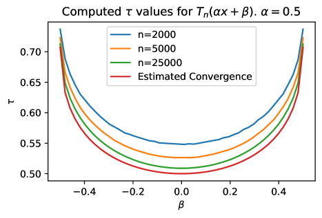
Figure 1. The computed values of $\tau_{0.5,{\beta}}$ for large degree $n$ along with the values from Conjecture 4.8, which the approximations seem to converge to.

4.3. Temporal Complexity

Now that we have results about how the degree changes as we subdivide, we can talk about the temporal complexity of the algorithm as a whole. At each step of the problem, we have $n$ polynomials where in coordinate $i$ each polynomial is degree at most $d_{i}$. Let $D=\prod_{i=1}^{n}(d_{i}+1)$ be the maximum number of coefficients in an approximation. The algorithm has two parts, the linear reduction method and the subdivision. We will ignore the elimination checks, as we assume those only speed things up.

The linear reduction method requires summing all the terms in the coefficients and solving an $n\times n$ system, with a complexity of $O(nD+n^{3})=O(nD)$.

The cost of reapproximating a system in coordinate $j$ is $O(n(d_{j}+1)D)$. So the subdivision cost dominates the temporal complexity for large degree. For simplicity, we approximate this subdivision cost as $(\sum_{i=1}^{n}d_{i})(\prod_{i=1}^{n}d_{i})$ or $nd^{n+1}$, if the degrees are all the same $d_{i}=d$.

After the first subdivision step the algorithm always splits the interval exactly in half, so we use $\tau$ to mean $\tau_{0.5}$. The cost of the next step is $n2^{n}(\tau d)^{n+1}$. The ratio of the cost of each step to the cost of the previous step is then $\frac{n2^{n}(\tau d)^{n+1}}{nd^{n+1}}=2^{n}\tau^{n+1}\leq\sqrt{2}^{n-1}$, by Corollary 4.7. The number of steps required will be roughly $2\log_{2}{d}$. For $n=1$, each step has the same cost so the total complexity is $O(d^{2}\log{d})$. For $n>1$, the complexity is dominated by the final step, so is $nd^{n+1}(\sqrt{2}^{n-1})^{2\log_{2}{d}}=nd^{2n}$. So for $n>1$ we have complexity $O(nd^{2n})$.

4.4. Temporal Complexity Numerical Results

In general the complexity will be better than that shown above because $\tau$ is often less than $\frac{\sqrt{2}}{2}$. Intervals on the interior have significantly lower degree than those on the edge. This is shown in Table 1, where we show the degree of $T_{10000}(x)$ on four rounds of subdivision (with $\alpha=0.5$). Note that the intervals near $0$ scale by roughly ${\alpha}$, as would be expected from Theorem 4.6.

7173
2730				5104
1375		1469		1738		3633
718	728	750	791	853	964	1194	2589

Table 1. The $i$th row of this table gives the degree when approximating $T_{10000}$ on the $2^{i-1}$ evenly spaced intervals on $[0,1]$. The leftmost columns are the intervals closest to $0$, the rightmost those closest to $1$. The degrees on $[-1,0]$ are the same (in reversed order to make them symmetrical about $0$). The degree of the approximations near $0$ (the left side of this table) scale approximately like $\alpha=\frac{1}{2}$, as would be expected from Theorem 4.6. The degree on the intervals nearest $1$ scale more like our worst-case bound of $\sqrt{\alpha}$.

Dim	Step 2	Step 3	Step 4	Step 5	Step 6
1	1.	0.63246763	0.36532202	0.20318345	0.11092983
2	1.41421356	0.9580105	0.56098545	0.31115873	0.16892276
3	2.	1.45111635	0.86144459	0.47651401	0.25723376
4	2.82842712	2.19803297	1.32282715	0.72974201	0.39171281

Table 2. The relative complexities of the first steps of solver relative to the first step.

Because of this, the complexity should actually be much better than our estimate $O(nd^{2n})$ above. Assuming the degrees actually drop as predicted by Conjecture 4.8, we get the following conjecture, which is supported by Table 2.

Conjecture 4.9.

For any dimension $n$, and sufficiently large degree $d$, for a system of $n$ degree-$d$ Chebyshev polynomials in $n$ variables, the cost of subdivision will be greatest on the second step, which will be $\sqrt{2}^{n-1}$ times the complexity of the first step.

The complexity will then decrease with each step at an increasing rate, becoming $50\%$ cheaper at each step in the limit. Thus the temporal complexity of the entire algorithm should be the temporal complexity of the second step, which is $O(nd^{n+1}\sqrt{2}^{n})$.

This means that in one dimension our solver has complexity $O(d^{2})$. A common alternative method for solving a single one-dimensional Chebyshev polynomial is to find the eigenvalues of the colleague matrix, which has complexity $O(d^{3})$. Recently eigenvalue-based solvers have been developed in one dimension that are $O(d^{2})$ [15]. In higher dimensions, the eigenvalue-based methods use the Macaulay matrix, and, as shown in [16] these methods have a temporal complexity that is at best $O(d^{3n})$.

5. Stability Analysis

We do not present a rigorous treatment of the stability of this algorithm, but we can give reasoning and numerical evidence that the suggest that this algorithm can find roots with an extremely high degree of accuracy.

There are two principle steps in the algorithm at which we have to worry about error being introduced: first, transforming polynomials to new intervals and, second, zooming in to new intervals. Both of these are very well behaved in numerical tests, as discussed below.

5.1. Error of polynomial transformation

Transforming the polynomials to a new interval only requires a tensor multiplication of the Chebyshev transformation matrix by the polynomial tensor. Assume that $C_{n,m}({\alpha},{\beta})$ can be computed with maximum (entrywise) error of at most $\varepsilon_{C}$, each coefficient of our polynomials is bounded in magnitude by $N$, and the dimension we are transforming in has degree $D$. In this case the error introduced in the transformation is at most $\varepsilon_{C}ND$ for each coefficient. So if we know what $\varepsilon_{C}$ is, we can bound this error and add it to the tracked approximation error at each step.

5.1.1. Stability of recurrence relation

While we can not currently prove any useful bounds on the error involved in creating the Chebyshev transformation matrix, there are a few reasons (listed below) to believe it should be well behaved numerically. Additionally, the results of numerical experiments seem to show that it is well behaved.

First, the following theorem shows the terms in the matrix are bounded in magnitude by $2$. Therefore, it seems like the recurrence relation in (4) is most likely stable and any errors that are introduced won’t grow.

Theorem 5.1.

If $\lvert{\alpha}\rvert+\lvert{\beta}\rvert\leq 1$, then $\lvert{C}_{n,m}({\alpha},{\beta})\rvert\leq\begin{cases}1&n=0\\ 2&\text{otherwise}\end{cases}$

Proof.

From theorem 3.1 in [8] we have that

$$\int_{-1}^{1}\frac{f(x)T_{k}(x)}{\sqrt{1-x^{2}}}dx=a_{k}{\kappa}_{k}\text{ where }{\kappa}_{k}=\begin{cases}\pi&k=0\\ \frac{\pi}{2}&\text{otherwise}\end{cases}$$

Substituting $x=cos(\theta)$ gives

(8) $$a_{k}=\int_{0}^{\pi}\frac{f(\cos(\theta))T_{k}(\cos(\theta))\sin(\theta)}{\gamma_{k}\sqrt{1-\cos^{2}(\theta)}}d\theta=\int_{0}^{\pi}\frac{f(\cos(\theta))\cos(k\theta)}{\gamma_{k}}d\theta$$

Thus we have

$${C}_{n,m}({\alpha},{\beta})=\int_{0}^{\pi}\frac{T_{m}({\alpha}\cos(\theta)+{\beta})\cos(n\theta)}{\gamma_{n}}d\theta$$

If $\lvert{\alpha}\rvert+\lvert{\beta}\rvert\leq 1$ the numerator is bounded in magnitude by 1, so

$$\lvert{C}_{n,m}({\alpha},{\beta})\rvert\leq\frac{\pi}{{\kappa}_{n}}=\begin{cases}1&n=0\\ 2&\text{otherwise.}\end{cases}$$

∎

Also, it is easy to verify from (4) that if $M_{k}$ is the sum of the entries in column $k$, that $M_{k+1}=2({\alpha}+{\beta})M_{k}-M_{k-1}$. This has the characteristic equation $\lambda^{2}-2({\alpha}+{\beta})\lambda+1=0$, with eigenvalues $\lambda={\alpha}+{\beta}\pm\sqrt{({\alpha}+{\beta})^{2}-1}$. For ${\alpha}+{\beta}\leq 1$, $\lvert\lambda\rvert=1$. So if errors are introduced the sums of the errors in the columns will stay small. This doesn’t guarantee the magnitude of the individual entries will stay small, but that seems likely. Finally, similarity can be seen between the recurrence relation and Clenshaw’s algorithm, which is known to be stable [17]. We expect an analysis similar to that of Clenshaw’s algorithm could be used to prove stability of the matrix creation.

We can also estimate the error of creating the Chebyshev transformation matrix by creating it with extra digits of precision and comparing to the floating point result. Randomly choosing $1000$ values of $\alpha$ from $\operatorname{Uniform}(0,1)$ and $\beta$ from $\operatorname{Uniform}(0,\alpha)$, the maximum error observed in any entry of any matrix up to column $100$ is $3.82\text{\times}{10}^{-15}$. And for $C(\frac{1}{2},\frac{1}{2})$ which is the matrix used for splitting intervals, the error is $0$ until column 58.

5.2. Error of zooming in on intervals

The stability of this part of the algorithm depends on three main ideas. First, that the matrix ${A}$ we invert has similar conditioning to the Jacobian matrix $J$. Next, the accuracy of our algorithm only depends on not erroneously throwing out intervals, so we can avoid mistakes by not excluding any intervals when the condition number of ${A}$ is large. Finally, the error as we zoom in to smaller intervals scales, so that the relative error stays about the same. Each of these ideas is discussed in more detail in this section, but we do not give formal proofs of stability results here.

Inverting the matrix ${A}$ is necessary for determining the width of the interval for the next iteration. We should be wary of this inversion, especially because we expect the entries of ${A}$ to approach $0$ as we get closer to a root. One reason why this is not a serious problem in practice is that the terms of ${A}$ are the derivative of our functions at some point in the interval, so as we get closer to the root ${A}$ should be close to the Jacobian matrix $J$. So we can reasonably expect ${A}$ to be well-conditioned when $J$ is, which is approximately determined by the conditioning of the root-finding problem itself. (See Section 3 for details on why ${A}$ behaves as it does.)

One flaw in this reasoning is that when we scale the interval by ${\alpha}$ it will scale the $i$-th column of $J$ by ${\alpha}_{i}$. This means we could scale different dimensions by different amounts and potentially create an ill-conditioned matrix. This, however, is easily remedied by preconditioning ${A}$ with column scaling. In our implementation we scale by an appropriate power of $2$ to ensure that the maximum value in every column of $A$ is in the interval $[\frac{1}{2},1)$.

The accuracy of our algorithm from one iteration to the next is guaranteed as long as it returns any subinterval that contains the root. Since the transformation matrix is well-behaved, we can proceed confidently on this new subinterval. Thus, it isn’t vital that we exactly determine the optimal subinterval.

In order to guarantee that we don’t erroneously shrink an interval too much, we check the conditioning of ${A}$ as we solve, and when it’s poorly conditioned do not shrink further. We continue instead by subdividing and applying the exclusion checks to the subintervals.

Finally, consider the propagation of a small absolute error from the initial approximation or trimming nearly-zero coefficients. Although this small error is initially insignificant, it could grow as we zoom in and the values of ${A}$ shrink. But if at one iteration we scale our interval by ${\alpha}$, we expect the entries of ${A}$ to also scale by ${\alpha}$, and the relative error increases by $\frac{1}{{\alpha}}$ an interval of size ${\alpha}$. This means that the total contribution of this scaled error to the problem on the whole interval remains relatively constant.

Finally, we observe that the algorithm converges quadratically and so will only have a few steps at which it can add any error at all.

6. Numerical Tests

6.1. Chebyshev Polynomial Solver

In this subsection we present timing and accuracy results of the Chebyshev polynomial solver part of our method, without the approximator. To do this we must start with polynomials already expressed in the Chebyshev basis.

6.1.1. Accuracy

The Python implementation of our solver is more accurate than some of the built-in (standard library) functions in Python, and often gives results that are the best possible in double precision (the precision in which we have implemented this), meaning that that the zeros found by our algorithm are the closest possible floating point number to the true zero.

As an example to illustrate this, consider finding the zeros of $T_{1000}(x)$. This is an easy problem analytically because we know the zeros are at $x=\cos{(\frac{k+0.5}{1000}\pi)}$ for $k=0,1,\dots,999$. However, the numerical error of computing these cosine values of $x$ in Python (using the default double precision) is only accurate to within $4\text{\times}{10}^{-16}$. This may seem insignificant, but our algorithm computes all the zeros to within $6\text{\times}{10}^{-17}$, and $943$ of them are the closest floating point value to the actual zero. So naïvely comparing our solutions to the numerically computed values of $x=\cos{(\frac{k+0.5}{1000}\pi)}$ does not adequately reflect the accuracy of our results.

The best way we have found of examining the accuracy of the zeros found with our solver is to Newton polish the zeros using $50$ digits of precision in Python’s mpmath library. We then can report the distance from the found zeros to the high precision polished zero. But, when doing this, it is useful to remember that the best possible error solution is given by the floating point number closest to the true zero, which has an error not more than $2^{-54}$ ($5.55\text{\times}{10}^{-17}$) for numbers between $0$ and $1$. For example, in Figure 6.1.1 we plot (in blue) a histogram for the errors of the zeros found by our algorithm for every Chebyshev monomial $T_{d}(x)$ of degree $d=1$ to $d=1000$. On the $x$-axis is the size of the error, and on the $y$-axis is the density of found zeros with that error. On the same plot, we plot (in black) the density of errors of the closest floating point numbers, that is, the distance from the true zero to the closest floating point number. These are very similar, and indeed $92.9\%$ of the zeros found by our algorithm were the closest floating point number to the true zero—that is, our computed zeros were the best possible numerical solution. The worst error for any of our computed zeros is $1.5\text{\times}{10}^{-16}$.

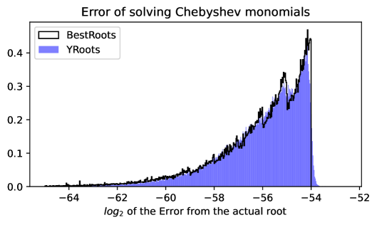
Figure 2. Histogram (in blue) of the errors (distance to the true value) for all of the zeros computed by our algorithm for the first $1000$ Chebyshev monomials $T_{d}(x)$. The $x$-axis is the size of the error, and the $y$-axis is the density of the zeros with that error. Plotted in black is the density of the errors of the best-possible numerical solutions (the nearest floating-point number to the true zero).

In higher dimensions our implementation of the polynomial solver (without the approximator) also has good accuracy finding the zeros of random Chebyshev polynomials; numerical results are plotted in Figure 3.

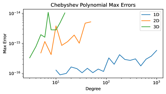
Figure 3. Maximum error on all the zeros computed by our algorithm compared to the true zeros of systems of polynomials of varying total degree with coefficients drawn form the standard normal distribution.

6.1.2. Timing

Timing results of numerical tests of polynomial systems of increasing degree ${d}$ in dimensions $1$, $2$, and $3$, appears to be better even than the conjectured temporal complexity of $O(nd^{n+1}\sqrt{2}^{n})$, as shown in Figure 4.

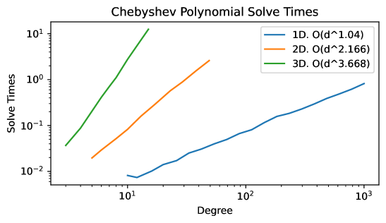
Figure 4. Average time to solve 10 systems of varying total degree ${d}$ with coefficients drawn form the standard normal distribution in dimensions $1$, $2$, and $3$. As functions of ${d}$ these are appear to be better even than the conjectured temporal complexity of $O(nd^{n+1}\sqrt{2}^{n})$.

6.2. Full YRoots Solver: Comparison to Other Methods

On a range of tests, which we describe below, we compared the speed and accuracy of the Python implementation of our algorithm, which we call YRoots, with the following solvers: Bertini [4], which uses a homotopy method; the eigenvalue-based solver of Telen et al. [6], implemented in Julia; Chebfun2 (in two dimensions only), which uses Chebyshev proxy and subdivision, as we do, but then uses Bezout resultants to solve the systems on subintervals, and is implemented in MATLAB; and Mathematica’s Reduce and NSolveValues. All tests were run on the same machine (a PowerEdge R640 with Intel Xeon Gold 6248 CPU server, 80 cores, and 768GiB RAM).

Our main test collections were the Chebfun Test Suite [18] in two dimensions only; a collection of several systems of transcendental functions in $3$ and $4$ dimensions that we constructed, somewhat arbitrarily; and a collection of randomly generated polynomials in each dimension of varying degrees.

6.2.1. Random Polynomial Times

In each dimension we generated $300$ polynomials for the random polynomial tests by drawing coefficients for the power-basis (standard monomials of the form $x_{1}^{k_{1}}\cdots x_{n}^{k_{n}}$) from the standard normal distribution, but setting the constant term to $0$ to ensure that there would be at least one zero in the standard interval $[-1,1]^{n}$.

The timing results on the random polynomials are summarized in Figures 5 and 6. For higher degrees (more than degree $10$ in $2$ dimensions and more than degree $5$ in $3$ dimensions) our YRoots solver is substantially faster than all the other solvers. We expect that implementing YRoots in a faster language like Julia or C would make it much faster and competitive with Telen’s solver (written in Julia) in those low-degree cases.

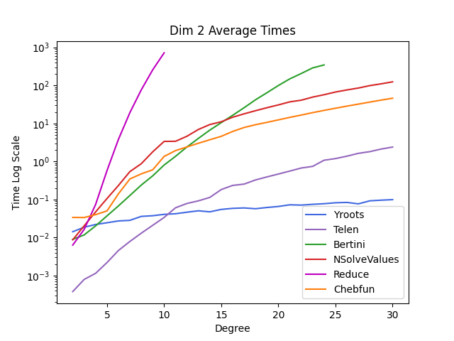
Figure 5. The results of running the random-polynomial tests in 2-dimensions from degree 2–30, with degree on the $x$-axis and the timing in log scale on the $y$-axis, and each of the different methods plotted as a different colored line. We expect that implementing YRoots in a faster language like Julia or C would make it competitive with Telen in degree less than 10.

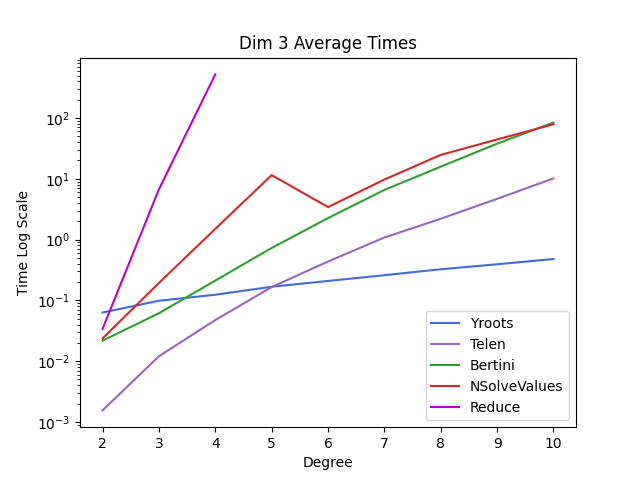
Figure 6. The results of running the random-polynomial tests in 3-dimensions and degrees 2–9, with degree on the $x$-axis and the timing in log scale on the $y$-axis, and each of the different methods plotted as a different colored line. Note that Chebfun is not included because it is not yet implemented in more than 2 dimensions. Again, we expect that a Julia implementation of YRoots instead of its current Python implementation would be competitive with Telen in low degrees.

6.2.2. Avoids Undesired Zeros

One reason our YRoots solver is faster than Bertini and the Telen solver is that YRoots only solves for real zeros inside a given bounded interval (in these tests that is the standard interval $[-1,1]^{n}$, while both of those other methods attempt to find all the zeros in $\mathbb{C}^{n}$. Chebfun2 uses subdivision to reduce the degree of the Chebyshev approximation on each interval, which may allow it to avoid searching for some of the unwanted zeros of the original system, but it also uses resultants to find the zeros of the approximation on each subinterval, and resultants also often finds additional nonreal zeros (which are then discarded by Chebfun2).

For the purposes of our testing, we ran NSolveValues and Reduce restricted to the standard interval, but they do have the capability to find zeros globally as well.

The fact that Telen and Bertini (and, to some extent Chebfun2), find more zeros than is needed probably contributes significantly to their completion time, especially in higher-dimensions and higher degree. We consider it an advantage that our algorithm only finds real zeros on the interval of interest rather than spending resources finding unwanted zeros.

6.2.3. Random Polynomial Accuracy

To evaluate the accuracy of the the computed zeros in the random polynomial tests, we use residuals, which are the values of the functions at the computed zeros. If a computed zero is perfectly correct, then the residual should be zero.

The maximum (worst) residuals for each solver in each degree in the polynomial tests in dimensions 2 and 3 are plotted in Figures 7 and 8. Most of the solvers, including YRoots, have consistently good results, but Telen’s solver is consistently worse than most of the others by a factor of about 100 and NSolveValues has terrible performance in low degrees, but much better once the degree is large enough. We don’t know why this happens.

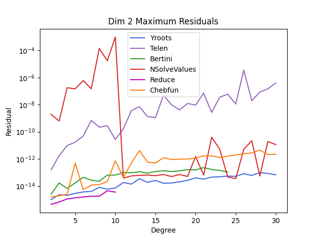
Figure 7. The maximum (worst) residuals of for the different solvers in on the 2-dimensional random-polynomial tests, with degree on the $x$-axis and the residual in log scale on the $y$-axis, and each of the different methods plotted as a different colored line. Reduce is only plotted to degree 10, because in higher degrees it took too long to finish. We don’t know how to explain the very poor performance of NSolveValues in low degree and yet good performance in higher degrees.

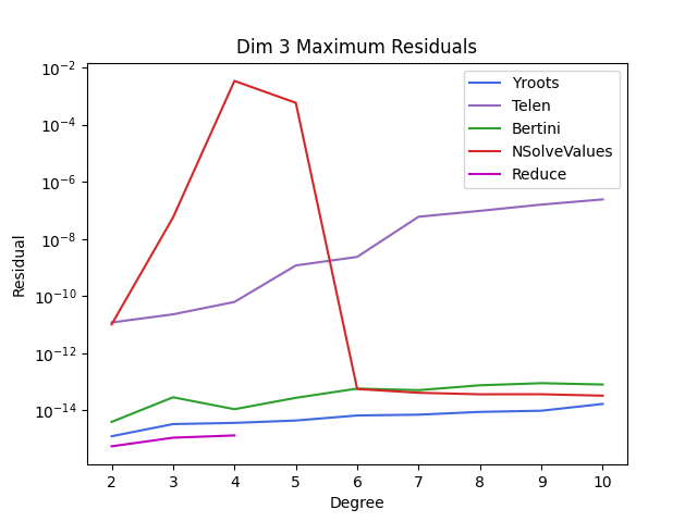
Figure 8. The maximum (worst) residuals of for the different solvers in on the 3-dimensional random-polynomial tests, with degree on the $x$-axis and the residual in log scale on the $y$-axis, and each of the different methods plotted as a different colored line. Reduce is only plotted to degree 4, because in higher degrees it took too long to finish. Again, we observe, but cannot explain, the very bad performance of NSolveValues in low degree.

6.2.4. Chebfun Test Suite and 3-Dimensional Transcendental Tests

We ran timing and residual tests for the various solvers on the Chebfun test suite, which is purely 2-dimensional, and the 3- and 4-dimensional transcendental tests.

Although some of the Chebfun Test Suite involves systems of power-basis polynomials, others involve non-polynomial functions. Bertini and Telen’s solver are not included in these results because they only work on polynomials expressed in the power basis.

Timing results are plotted in Figures 9, 10, and 11.

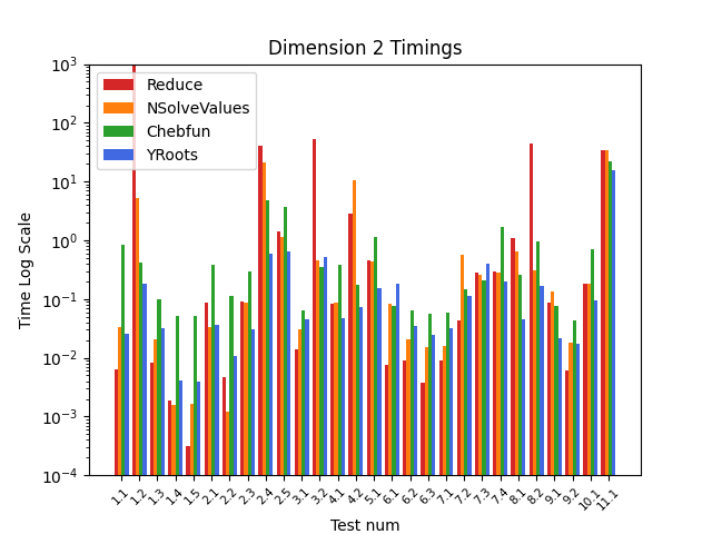
Figure 9. Time to solve each of the Chebfun Test Suite tests, using each of the solvers that work with non-polynomial functions. Reduce failed to solve Test 1.2 at all, resulting in a time of $\infty$.

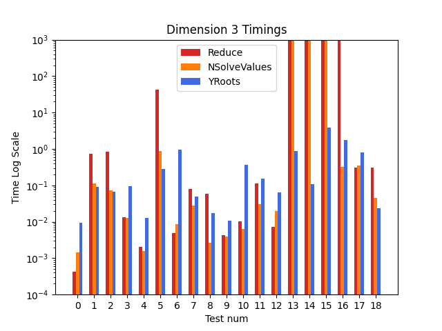
Figure 10. Time to solve each of our 3-dimensional transcendental tests, using each of the solvers that work with non-polynomial functions. Bars that run off the top of the chart chart indicate that the corresponding solver failed to solve the problem at all.

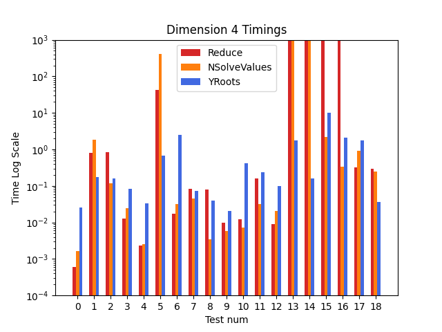
Figure 11. Time to solve each of our 4-dimensional transcendental tests, using each of the solvers that work with non-polynomial functions. Bars that run off the top of the chart chart indicate that the corresponding solver failed to solve the problem at all.

Accuracy (residual) results are plotted in Figures 12, 13, and 14.

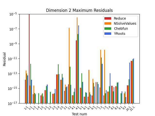
Figure 12. Residuals on each of the Chebfun Test Suite tests, using each of the solvers that work with non-polynomial functions. Note that Reduce failed to solve Test 1.2 entirely, so its residual is plotted as infinite.

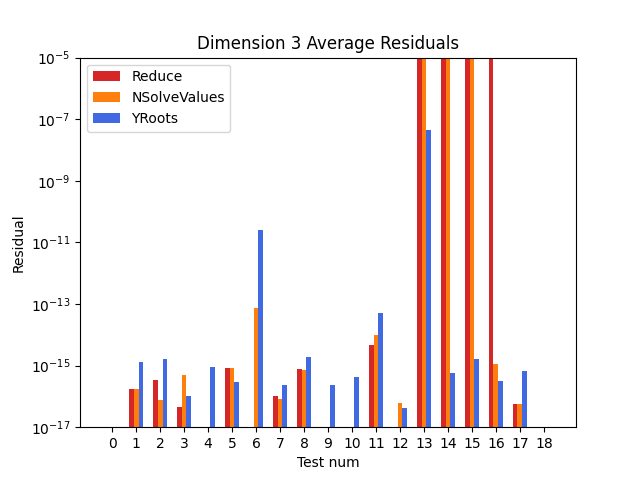
Figure 13. Residuals for each of our 3-dimensional transcendental tests, using each of the solvers that work with non-polynomial functions. Bars that run off the top of the chart chart indicate that the corresponding solver failed to solve the problem at all.

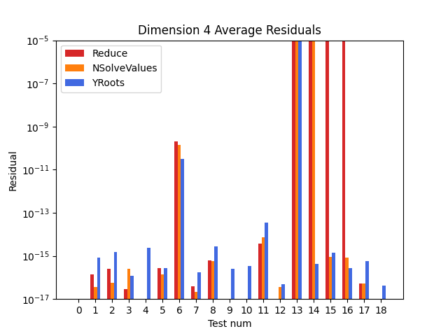
Figure 14. Maximum residuals on each of our 4-dimensional transcendental tests, using each of the solvers that work with non-polynomial functions. Bars that run off the top of the chart indicate that the corresponding solver failed to solve the problem at all.

7. Conclusion

Our novel Chebyshev polynomial solver is able to find common zeros with extreme accuracy, with comparable or better speed then existing methods. It works especially well through dimension 3. We are still testing its performance in higher dimensions. When combined with existing Chebyshev approximation methods, it can find common zeros of almost any sufficiently smooth system of equations.

There are many potential improvements that could be made to further improve the algorithm. Better elimination checks or reduction methods could speed up the solver. Using the low rank approximation methods of Chebfun might speed up solve time in higher dimensions. Finding a way to do fast multiplication by the Chebyshev transformation matrix would also significantly increase the speed of the algorithm.

Appendix A Proofs of Lemmas

A.1. Proof of Lemma 4.4

Proof.

For the ${\beta}=0$ case, we use the ellipse definition $\frac{x^{2}}{a^{2}}+\frac{y^{2}}{b^{2}}=1$ where $2a$ and $2b$ are the width and height of the ellipse. Thus $y=\pm b\sqrt{1-\frac{x^{2}}{a^{2}}}$, $\frac{dy}{dx}=\frac{-b\frac{2x}{a}}{\sqrt{a^{2}-x^{2}}}$. So if we have two ellipses centered at $0$ with the same height, the one with the greater width will decrease slower, and thus fully contain the other one. So if $2b=q-q^{-1}={\alpha}(p-p^{-1})$, then $E_{q}$ is contained in ${\alpha}E_{p}$, and it intersects it so is the smallest such $q$.

For the ${\beta}=1-{\alpha}$ case, note the if $q+q^{-1}={\alpha}(p+p^{-1})+2{\beta}$, then $E_{q}$ and ${\alpha}E_{p}+{\beta}$ both have a foci of $1$. Call this foci $F$. Let the other foci of $E_{q}$ by $F_{1}$, and the other foci of ${\alpha}E_{p}+{\beta}$ $F_{2}$. Let the intersection of the ellipses on the x axis be $P$. The sum of the distances from the foci to any point on the ellipse is constant for an ellipse. So for any point $Q$, $\lvert F_{1}Q\rvert+\lvert FQ\rvert=\lvert F_{1}P\rvert+\lvert FP\rvert$ and $\lvert F_{2}Q\rvert+\lvert FQ\rvert=\lvert F_{2}P\rvert+\lvert FP\rvert$. So $\lvert F_{1}Q\rvert-\lvert F_{2}Q\rvert=\lvert F_{1}P\rvert-\lvert F_{2}P\rvert$. As $F_{1}$, $F_{2}$ and $P$ are co-linear, $\lvert F_{1}Q\rvert=\lvert F_{1}F_{2}\rvert+\lvert F_{2}Q\rvert$. So we get $\lvert F_{1}F_{2}\rvert=\lvert F_{1}F_{2}\rvert+\lvert F_{2}Q\rvert$. By the triangle inequality this will only be true on the $x$-axis, and everywhere else $E_{q}$ will be outside of ${\alpha}E_{p}+{\beta}$. ∎

A.2. Proof of Theorem 4.6

Proof.

Lemma 4.5 gives $\tau_{{\alpha},{\beta}}\leq\inf_{p>1}\frac{\log{(q})}{\log{(p)}}$. And Lemma 4.4 implies that if ${\beta}=0$, then $t=\frac{1}{2}(q-q^{-1})=\frac{{\alpha}}{2}(p-p^{-1})$ for $t>0$. Thus $q=t+\sqrt{t^{2}+1}$. $p=\frac{t}{{\alpha}}+\sqrt{(\frac{t}{{\alpha}})^{2}+1}$. $\tau_{{\alpha},0}\leq\inf_{t>0}\frac{\log{(t+\sqrt{t^{2}+1})}}{\log{(\frac{t}{{\alpha}}+\sqrt{(\frac{t}{{\alpha}})^{2}+1})}}\leq\lim_{t\to 0}\frac{\log{(t+\sqrt{t^{2}+1})}}{\log{(\frac{t}{{\alpha}}+\sqrt{(\frac{t}{{\alpha}})^{2}+1})}}=\lim_{t\to 0}\frac{\log{(t+1+\frac{t^{2}}{2})}}{\log{(\frac{t}{{\alpha}}+1+\frac{t^{2}}{2{\alpha}^{2}})}}=\lim_{t\to 0}\frac{\log{(1+t)}}{\log{(1+\frac{t}{{\alpha}})}}=\lim_{t\to 0}\frac{t}{\frac{t}{{\alpha}}}={\alpha}$.

Lemma 4.4 implies that if ${\beta}=1-{\alpha}$, then $t=\frac{1}{2}(q+q^{-1})=\frac{{\alpha}}{2}(p+p^{-1})+{\beta}$ for $t>1$. So $q=t+\sqrt{t^{2}-1}$. $p=\frac{t-{\beta}}{{\alpha}}+\sqrt{(\frac{t-{\beta}}{{\alpha}})^{2}-1}$. $\tau_{{\alpha},1-{\alpha}}\leq\inf_{t>1}\frac{\log{(t+\sqrt{t^{2}-1})}}{\log{(\frac{t-{\beta}}{{\alpha}}+\sqrt{(\frac{t-{\beta}}{{\alpha}})^{2}-1})}}$. Letting $t=1+\varepsilon$, gives $\tau_{{\alpha},1-{\alpha}}\leq\lim_{\varepsilon\to 0}\frac{\log{(1+\varepsilon+\sqrt{2\varepsilon+\varepsilon^{2}})}}{\log{(1+\frac{\varepsilon}{{\alpha}}+\sqrt{2\frac{\varepsilon}{{\alpha}}+(\frac{\varepsilon}{{\alpha}})^{2}})}}=\lim_{\varepsilon\to 0}\frac{\log{(1+\varepsilon+\sqrt{2\varepsilon})}}{\log{(1+\frac{\varepsilon}{{\alpha}}+\sqrt{2\frac{\varepsilon}{{\alpha}}})}}=\lim_{\varepsilon\to 0}\frac{\varepsilon+\sqrt{2\varepsilon}}{\frac{\varepsilon}{{\alpha}}+\sqrt{2\frac{\varepsilon}{{\alpha}}}}=\sqrt{{\alpha}}$. ∎

References

-
[1]
J. P. Boyd, Solving
transcendental equations, Society for Industrial and Applied Mathematics,
Philadelphia, PA, 2014, the Chebyshev polynomial proxy and other numerical
rootfinders, perturbation series, and oracles.
doi:10.1137/1.9781611973525.
URL https://doi.org/10.1137/1.9781611973525 -
[2]
A. Townsend, Chebfun2:
Rootfinding and optimisation, in: N. H. T. A. Driscoll, L. N. Trefethen
(Eds.), Chebfun Guide, Pafnuty Publications, 2014.
URL https://www.chebfun.org/docs/guide/guide14.html -
[3]
B. Mourrain, J. Pavone,
Subdivision
methods for solving polynomial equations, Journal of Symbolic Computation
44 (3) (2009) 292–306, polynomial System Solving in honor of Daniel Lazard.
doi:https://doi.org/10.1016/j.jsc.2008.04.016.
URL https://www.sciencedirect.com/science/article/pii/S0747717108001168 - [4] D. J. Bates, J. D. Hauenstein, C. W. Sommese, Andrew J.and Wampler, Bertini: Software for numerical algebraic geometry, http://dx.doi.org/10.7274/R0H41PB5.
- [5] H. J. Stetter, Numerical polynomial algebra, Vol. 85, Siam, 2004.
-
[6]
B. Mourrain, S. Telen, M. Van Barel,
Truncated normal forms for
solving polynomial systems: generalized and efficient algorithms, J.
Symbolic Comput. 102 (2021) 63–85.
doi:10.1016/j.jsc.2019.10.009.
URL https://doi.org/10.1016/j.jsc.2019.10.009 -
[7]
A. Rababah, Transformation of
Chebyshev-Bernstein polynomial basis, Comput. Methods Appl. Math. 3 (4)
(2003) 608–622.
doi:10.2478/cmam-2003-0038.
URL https://doi.org/10.2478/cmam-2003-0038 - [8] L. N. Trefethen, Approximation Theory and Approximation Practice, Extended Edition, SIAM-Society for Industrial and Applied Mathematics, Philadelphia, PA, USA, 2019.
-
[9]
J. P. Boyd,
Finding
the zeros of a univariate equation: proxy rootfinders, chebyshev
interpolation, and the companion matrix., SIAM Review 55 (2) (2013) 375.
URL https://www.lib.byu.edu/cgi-bin/remoteauth.pl?url=http://search.ebscohost.com/login.aspx?direct=true&db=msn&AN=MR3049926&site=ehost-live&scope=site -
[10]
A. Townsend, L. N. Trefethen, An
extension of chebfun to two dimensions, SIAM Journal on Scientific Computing
35 (6) (2013) C495–C518.
arXiv:https://doi.org/10.1137/130908002, doi:10.1137/130908002.
URL https://doi.org/10.1137/130908002 -
[11]
B. Hashemi, L. N. Trefethen, Chebfun
in three dimensions, SIAM Journal on Scientific Computing 39 (5) (2017)
C341–C363.
arXiv:https://doi.org/10.1137/16M1083803, doi:10.1137/16M1083803.
URL https://doi.org/10.1137/16M1083803 -
[12]
H. Robbins, A remark on stirling’s
formula, The American Mathematical Monthly 62 (1) (1955) 26–29.
URL http://www.jstor.org/stable/2308012 -
[13]
Y. Nakatsukasa, V. Noferini, A. Townsend,
Computing the common zeros
of two bivariate functions via bézout resultants, Numerische Mathematik
129 (1) (2015) 181–209.
doi:10.1007/s00211-014-0635-z.
URL https://doi.org/10.1007/s00211-014-0635-z - [14] S. Bernstein, Sur l’ordre de la meilleure approximation des fonctions continues par des polynomes de degrè donnè, Academie Royale de Belgique Memoires 4 (1912) 1–104.
- [15] K. Serkh, V. Rokhlin, A provably componentwise backward stable qr algorithm for the diagonalization of colleague matrices (2021). arXiv:2102.12186.
- [16] S. Parkinson, H. Ringer, K. Wall, E. Parkinson, L. Erekson, D. Christensen, T. J. Jarvis, Analysis of normal-form algorithms for solving systems of polynomial equations (2021). arXiv:2104.03526.
-
[17]
A. Smoktunowicz, Backward
stability of clenshaw’s algorithm, BIT 42 (3) (2002) 600–610.
doi:10.1023/A:1022001931526.
URL https://doi.org/10.1023/A:1022001931526 -
[18]
A. Townsend,
Chebfun2
rootfinding test suite, in: N. H. T. A. Driscoll, L. N. Trefethen (Eds.),
Chebfun Github Repository, Github, 2015.
URL https://github.com/chebfun/chebfun/tree/master/tests/chebfun2v