Spatiotemporal Monitoring of Epidemics via Solution of a Coefficient Inverse Problem

Abstract

Let S,I and R be susceptible, infected and recovered populations in a city affected by an epidemic. The SIR model of Lee, Liu, Tembine, Li and Osher, SIAM J. Appl. Math., 81, 190–207, 2021 of the spatiotemoral spread of epidemics is considered. This model consists of a system of three nonlinear coupled parabolic Partial Differential Equations with respect to the space and time dependent functions S,I and R. For the first time, a Coefficient Inverse Problem (CIP) for this system is posed. The so-called “convexification” numerical method for this inverse problem is constructed. The presence of the Carleman Weight Function (CWF) in the resulting regularization functional ensures the global convergence of the gradient descent method of the minimization of this functional to the true solution of the CIP, as long as the noise level tends to zero. The CWF is the function, which is used as the weight in the Carleman estimate for the corresponding Partial Differential Operator. Numerical studies demonstrate an accurate reconstruction of unknown coefficients as well as S,I,R functions inside of that city. As a by-product, uniqueness theorem for this CIP is proven. Since the minimal measured input data are required, then the proposed methodology has a potential of a significant decrease of the cost of monitoring of epidemics.

Key Words: monitoring epidemics, SIR model, coefficient inverse problem, Carleman estimate, convexification, global convergence, numerical studies

2020 Mathematics Subject Classification: 92D30, 35R30, 65M32.

1 Introduction

The experience of the COVD-19 pandemic demonstrates, in particular, the importance of the mathematical modeling of the spread of epidemics. The commonly used model is the model of Kermack and McKendrick, which was proposed in 1927 [13]. However, since this model is based on a system of three coupled Ordinary Differential Equations, then it describes only the total number of susceptible (S), infected (I) and recovered (R) populations, the so-called “SIR model”. On the other hand, recently Lee, Liu, Tembine, Li and Osher [26] have extended the SIR model of [13] to the case of a system of three nonlinear coupled parabolic Partial Differential Equations (PDEs), which we call again “SIR model”. The advantage of [26] over [13] is that the model of [26] governs both spatial and time dependencies of SIR populations. Thus, it makes sense to use this model for monitoring of both pointwise and timewise distributions of SIR populations. To decrease the cost, it is desirable to decrease the number of measurements. Results of the current paper indicate that it is possible to achieve this goal.

Let $\mathbf{x}=\left(x,y\right)\in\mathbb{R}^{2}$ be the vector of spatial variables and $t>0$ be time. The system of PDEs of [26] contains some parameters, which are actually unknown functions. These parameters are the infection rate $\beta\left(\mathbf{x},t\right),$ the recovery rate $\gamma\left(\mathbf{x},t\right)$ and three 2D vector functions $q_{S}\left(\mathbf{x},t\right),q_{I}\left(\mathbf{x},t\right)$ and $q_{R}\left(\mathbf{x},t\right),$ which are velocities of propagations of S, I and R populations respectively. Therefore, these functions are subjects to the solutions of certain Coefficient Inverse Problems (CIPs). This is the first work concerning a CIP for the SIR system of [26]. Hence, as in any first work about an applied problem, it is natural to introduce some simplifications. More precisely, we assume that the unknown coefficients $\beta$ and $\gamma$ depend only on $\mathbf{x}$, i.e. $\beta=\beta\left(\mathbf{x}\right)$ and $\gamma=\gamma\left(\mathbf{x}\right).$ In addition, we assume that the 2D vector functions $q_{S}\left(\mathbf{x}\right),q_{I}\left(\mathbf{x}\right)$,$q_{R}\left(\mathbf{x}\right)$ of velocities are known and depend only on $\mathbf{x}$. More complicated cases can be considered later. We assume that

$$\beta\left(\mathbf{x}\right),\gamma\left(\mathbf{x}\right)\in C\left(\overline{\Omega}\right);\text{ }q_{S}\left(\mathbf{x}\right),q_{I}\left(\mathbf{x}\right),q_{R}\left(\mathbf{x}\right)\in C^{1}\left(\overline{\Omega}\right),$$ (1.1)

where $\Omega\subset\mathbb{R}^{2}$ is a bounded domain occupied by a city affected by an epidemic. Below $\partial\Omega$ is the piecewise smooth boundary of $\Omega.$ Thus, the CIP of this paper targets the simultaneous reconstruction of all components of the 5D vector function $\Phi\left(\mathbf{x},t\right),$

$$\Phi\left(\mathbf{x},t\right)=\left(\beta\left(\mathbf{x}\right),\gamma\left(\mathbf{x}\right),S\left(\mathbf{x},t\right),I\left(\mathbf{x},t\right),R\left(\mathbf{x},t\right)\right).$$ (1.2)

The input data are the minimal ones. This is a single measurement of the 3D vector function $\Psi\left(\mathbf{x}\right)=\left(S\left(\mathbf{x},t_{0}\right),I\left(\mathbf{x},t_{0}\right),R\left(\mathbf{x},t_{0}\right)\right)$ inside of that city at a single fixed moment of time $\left\{t=t_{0}>0\right\}$ as well as boundary measurements at $\partial\Omega$ of functions $S\left(\mathbf{x},t\right),I\left(\mathbf{x},t\right),R\left(\mathbf{x},t\right)$ and their normal derivatives. Normal derivatives are fluxes of SIR populations through the boundary of that city. In particular, fluxes can be assumed to be zeros, as in [26]. We do not impose this assumption in our theory, although we use it in computations. It is hardly practical to measure the S,I,R functions at $\left\{t=0\right\}.$ Indeed, the epidemic process is yet immature at small times, and the authorities do not even know about the existence of an epidemic at $t\approx 0.$

Currently measurements of SIR populations are carried out at many locations inside of a city affected by an epidemic, and at all times $t\in\left(t_{1},T\right),$ where $t_{1}>0$ is a certain moment of time when authorities start to fight that epidemic, and $T>t_{1}$ is also a certain moment of time. On the other hand, our technique provides an accurate reconstruction of the vector function $\Phi$ in (1.2) inside of the city for all times of interest by requiring measurements inside of that city only at a single moment of time $t_{0}\in\left(t_{1},T\right)$ and conducting the rest of the measurements only at the city’s boundary. Hence, our technique has a potential of a significant decrease of the cost of monitoring of epidemics.

All CIPs for PDEs are both ill-posed and nonlinear ones. The conventional approach to numerical solutions of CIPs is based on the optimization of a least squares mismatch functional, see, e.g. [1, 2, 7, 8, 10, 11, 12]. However, phenomena of the ill-posedness and the nonlinearity of CIPs cause the non-convexity of those functionals. In turn, this can lead to the presence of multiple local minima and ravines, posing a risk of these optimization-based methods becoming stuck, see, e.g. [32] for a good numerical example of multiple local minima. Consequently, to effectively compute numerical solutions with these conventional techniques, good initial guesses are necessary. However, this requirement is not often met in practical situations.

In this work we develop the so-called “convexification” numerical method for our CIP. The convexification is the concept for CIPs, which is based on Carleman estimates. This concept was originally designed in [17, 15] to avoid multiple local minima and ravines of conventional least squares mismatch functionals. Each new CIP requires its own version of the convexification. While the originating works [17, 15] where purely theoretical ones, more recently this research team has published a number of works, in which the analytical studies of several versions of the convexification are combined with numerical results for a variety of CIPs, see, e.g. [19]-[22]. In addition, the second generation of the convexification was developed, see, e.g. [5, 6, 4, 28, 27].

The convexification consists of two steps:

1. Step 1: This step involves the elimination of unknown coefficients from the governing systems, resulting in a boundary value problem for a system of nonlinear PDEs. In the case of time dependent data, Volterra-like integrals with respect to $t$ are also involved in this system.

2. Step 2: This step focuses on the numerical solution of the problem formulated in Step 1. The solution of this problem provides the solution for the original CIP.  To solve that problem, a least squares weighted Tikhonov-like functional is constructed. The key element of this functional is the presence in it of the Carleman Weight Function (CWF) in it, which is not the case of the classical Tikhonov regularization functional [33]. The CWF is the function, which is used as the weight in the Carleman estimate for the corresponding PDE operator. Furthermore, it is demonstrated numerically in many of our publications, such as, e.g. [20, 21] as well as in Test 1 in section 8 of this paper that the absence of the CWF significantly deteriorates the solution. The key result of the convergence analysis of any version of the convexification method is a theorem, which claims that, for a proper choice of parameters, that functional is strongly convex on a convex set of an arbitrary but fixed diameter $d>0$. Next, it is derived from this result that the gradient descent method of the minimization of that functional converges to the true solution of the CIP starting from an arbitrary point of that set, as long as the level of noise in the data tends to zero. Since smallness conditions are not imposed on $d$, then we call this property “global convergence”.

As a by-product, we obtain uniqueness theorem for our CIP. Uniqueness for similar CIPs for one parabolic PDE was previously proven in [14, 16], [BK, Theorem 1.10.7], [19, Theorem 3.4.3]. We also refer to the Lipschitz stability estimate of [35], which implies uniqueness. All these works use the framework of the paper [9], in which the tool of Carleman estimates was introduced in the theory of CIPs for the first time. The convexification method is a numerical development of the idea of [9], which was originally formulated for a purely theoretical purpose.

Remark 1.1. Since the CIP, which we consider, is a quite complicated one, then we simplify the presentation via assuming that our domain of interest $\Omega$ is a rectangle and all functions we work with are sufficiently smooth. It is well known that smoothness assumptions are not of a significant concern in the theory of CIPs, see, e.g. [29, 30], [31, Theorem 4.1].

All functions considered below are real valued ones. In section 2 we pose both forward and inverse problems. In section 3 we carry out the above Step 1. In section 4 we formulate the Carleman estimate we work with. In  section 5 we carry out the above Step 2: we construct that functional and formulate theorems of its global convergence analysis. We prove those theorems in sections 6 and 7. In section 8 we present our numerical experiments. Summary of results is given in section 9.

2 Statements of Forward and Inverse Problems

Let $N>1$ be an integer and $B$ be a Banach space with its norm $\left\|\cdot\right\|_{B}$. Denote

$$\left.\begin{array}[]{c}B_{N}=B\times B\times...\times B,\text{ }N\text{ times,}\\ \left\|u\right\|_{B_{N}}=\left(\sum\limits_{k=1}^{N}\left\|u_{k}\right\|_{B}^{2}\right)^{1/2},\text{ }\forall u=\left(u_{1},...,u_{N}\right)\in B_{N}.\end{array}\right.$$

Let $a,b,A>0$ be some numbers. Let the number $\eta\in\left(0,1\right).$ We set the domain $\Omega\subset\mathbb{R}^{2}$ as a rectangle,

$$\left.\begin{array}[]{c}\Omega=\left\{\mathbf{x}=\left(x,y\right):a<x<b,\left|y\right|<A\right\},\mbox{ }\\ \Gamma=\partial\Omega\cap\left\{x=b\right\},\\ Q_{T}=\Omega\times\left(0,T\right),\mbox{ }S_{T}=\partial\Omega\times\left(0,T\right),\mbox{ }\Gamma_{T}=\Gamma\times\left(0,T\right),\\ Q_{\eta T}=\Omega\times\left(\left(1-\eta\right)T/2,\left(1+\eta\right)T/2\right)\subset Q_{T}.\end{array}\right.$$ (2.1)

We now follow notations of [26]. Shifting time as $t^{\prime}=t-t_{1}$ and still keeping the same notation for time, we assume that $t\in\left(0,T\right).$ Let $\rho_{S}\left(\mathbf{x},t\right),\rho_{I}\left(\mathbf{x},t\right)$ and $\rho_{R}\left(\mathbf{x},t\right)$ are S,I and R populations respectively. Recall that the 2D vector functions $q_{S}\left(\mathbf{x}\right),q_{I}\left(\mathbf{x}\right)$,$q_{R}\left(\mathbf{x}\right)$ are velocities of movements of these populations. Let $\beta\left(\mathbf{x}\right)$ and $\gamma\left(\mathbf{x}\right)$ be the infection and recovery rates respectively. The initial boundary value problem for the spatial SIR model has the form [26, formulas (2.1)]:

$$\partial_{t}\rho_{S}-\frac{\eta_{S}^{2}}{2}\Delta\rho_{S}+\text{div}\left(\rho_{S}q_{S}\right)+\beta\left(\mathbf{x}\right)\rho_{S}\rho_{I}=0,\text{ }\left(\mathbf{x},t\right)\in Q_{T},$$ (2.2)

$$\partial_{t}\rho_{I}-\frac{\eta_{I}^{2}}{2}\Delta\rho_{I}+\text{div}\left(\rho_{I}q_{I}\right)-\beta\left(\mathbf{x}\right)\rho_{S}\rho_{I}=0,\text{ }\left(\mathbf{x},t\right)\in Q_{T},$$ (2.3)

$$\partial_{t}\rho_{R}-\frac{\eta_{R}^{2}}{2}\Delta\rho_{R}+\text{div}\left(\rho_{R}q_{R}\right)-\gamma\left(\mathbf{x}\right)\rho_{I}=0,\text{ }\left(\mathbf{x},t\right)\in Q_{T},$$ (2.4)

$$\partial_{n}\rho_{S}\mathbf{\mid}_{S_{T}}=g_{1}\left(\mathbf{x},t\right),\text{ }\partial_{n}\rho_{I}\mathbf{\mid}_{S_{T}}=g_{2}\left(\mathbf{x},t\right),\text{ }\partial_{n}\rho_{R}\mathbf{\mid}_{S_{T}}=g_{3}\left(\mathbf{x},t\right).$$ (2.5)

$$\rho_{S}\left(\mathbf{x},0\right)=\rho_{S}^{0}\left(\mathbf{x}\right),\text{ }\rho_{I}\left(\mathbf{x},0\right)=\rho_{I}^{0}\left(\mathbf{x}\right),\text{ }\rho_{R}\left(\mathbf{x},0\right)=\rho_{R}^{0}\left(\mathbf{x}\right),$$ (2.6)

where $\partial_{n}$ is the normal derivative. This is our forward problem. Functions $g_{1},g_{2},g_{3}$ are fluxes of those populations through the boundary, and they are set to zero in [26]. However, our theory can consider a more general case of non-zero fluxes. Here, $\eta_{S}^{2},\eta_{R}^{2},\eta_{R}^{2}>0$ are constant viscosity terms, which are added in [26] to regularize the system. To simplify the presentation, we assume below without any loss of generality that

$$\frac{\eta_{S}^{2}}{2}=\frac{\eta_{I}^{2}}{2}=\frac{\eta_{R}^{2}}{2}=c>0,$$ (2.7)

where $c$ is a number, although our theory can be easily extended to the case when condition (2.7) is not imposed. Suppose for a moment that the boundary $\partial\Omega$ is sufficiently smooth, so as functions $\beta\left(\mathbf{x}\right),\gamma\left(\mathbf{x}\right),q_{S}\left(\mathbf{x}\right),q_{I}\left(\mathbf{x}\right)$,$q_{R}\left(\mathbf{x}\right)$. Also, assume for a moment that Neumann boundary conditions (2.5) are replaced with the Dirichlet boundary conditions. Then Theorem 7.1 of Chapter 7 of [24] as well as some other techniques developed in this book apply that, under some additional conditions, including an upper bound on $T$ (because of the nonlinearity of this system), the so changed initial boundary value problem has unique solution $\left(\rho_{S},\rho_{I},\rho_{R}\right)\left(\mathbf{x}\text{,}t\right),$ which is sufficiently smooth in $\overline{Q}_{T}.$ We, however, assume below that the forward problem (2.2)-(2.6) has unique solution

$$\rho_{S}\left(\mathbf{x},t\right),\rho_{I}\left(\mathbf{x},t\right),\rho_{R}\left(\mathbf{x},t\right)\in C^{6,3}\left(\overline{Q}_{T}\right),$$ (2.8)

see Remark 1.1.

We now pose our Coefficient Inverse Problem. Without a loss of generality, it is convenient to assume that measurements of spatial distributions of SIR populations inside of the affected city are conducted at the moment of time $t_{0}=T/2.$

Coefficient Inverse Problem (CIP). Let

$$\rho_{S}\left(\mathbf{x},\frac{T}{2}\right)=p_{1}\left(\mathbf{x}\right),\text{ }\rho_{I}\left(\mathbf{x},\frac{T}{2}\right)=p_{2}\left(\mathbf{x}\right),\text{ }\rho_{R}\left(\mathbf{x},\frac{T}{2}\right)=p_{3}\left(\mathbf{x}\right),$$ (2.9)

$$\rho_{S}\mid_{\Gamma_{T}}=f_{1}\left(y,t\right),\rho_{I}\mid_{\Gamma_{T}}=f_{2}\left(y,t\right),\rho_{S}\mid_{\Gamma_{T}}=f_{1}\left(y,t\right),\left(y,t\right)\in\Gamma_{T}.$$ (2.10)

Assume that functions in the right hand sides of (2.9) and (2.10) are known. However, let initial conditions (2.6) be unknown. Assuming the smoothness conditions (1.1) and (2.8), find the vector function $\Phi\left(\mathbf{x},t\right)$ in (1.2), which is rewritten now as:

$$\Phi\left(\mathbf{x},t\right)=\left(\beta\left(\mathbf{x}\right),\gamma\left(\mathbf{x}\right),\rho_{S}\left(\mathbf{x},t\right),\rho_{I}\left(\mathbf{x},t\right),\rho_{R}\left(\mathbf{x},t\right)\right),\text{ }\left(\mathbf{x},t\right)\in Q_{T}.$$ (2.11)

Thus, conditions (2.5) and (2.10) mean that we measure fluxes of SIR populations at the entire boundary of the city, whereas the numbers of these populations are measured only at the part $\Gamma\subset\partial\Omega$ of the boundary, see (2.1). Hence, (2.5) and (2.10) are incomplete lateral Cauchy data. Conditions (2.9) mean that we measure spatial distributions of SIR populations inside that city at a single moment of time $t=T/2.$

3 Transformation

Following the first step mentioned in section 1, we now transform our CIP in a boundary value problem for a system of four coupled nonlinear integral differential equations containing Volterra integrals with respect to $t$. But this system should not contain unknown coefficients $\beta\left(\mathbf{x}\right)$ and $\gamma\left(\mathbf{x}\right).$Assume that in (2.9)

$$\left|p_{1}\left(\mathbf{x}\right)\right|,\left|p_{2}\left(\mathbf{x}\right)\right|\geq\kappa,\text{ }\mathbf{x}\in\overline{\Omega},$$ (3.1)

where $\kappa>0$ is a number. Setting in (2.2) and (2.4) $t=T/2$ and using (2.7), (2.9) and (3.1), we obtain

$$\beta\left(\mathbf{x}\right)=-\frac{1}{\left(p_{1}p_{2}\right)\left(\mathbf{x}\right)}\partial_{t}\rho_{S}\left(\mathbf{x},\frac{T}{2}\right)+\frac{1}{\left(p_{1}p_{2}\right)\left(\mathbf{x}\right)}\left[c\Delta p_{1}\left(\mathbf{x}\right)-\text{div}\left(p_{1}q_{S}\right)\left(\mathbf{x}\right)\right],$$ (3.2)

$$\gamma\left(\mathbf{x}\right)=\frac{1}{p_{2}\left(\mathbf{x}\right)}\partial_{t}\rho_{R}\left(\mathbf{x},\frac{T}{2}\right)-\frac{1}{p_{2}\left(\mathbf{x}\right)}\left[c\Delta p_{3}\left(\mathbf{x}\right)-\text{div}\left(p_{3}q_{R}\right)\left(\mathbf{x}\right)\right].$$ (3.3)

Introduce new functions $v_{i}\left(\mathbf{x,}t\right),$ $i=1,2,3,$

$$\left.\begin{array}[]{c}v_{1}\left(\mathbf{x,}t\right)=\partial_{t}\rho_{S}\left(\mathbf{x,}t\right),v_{2}\left(\mathbf{x,}t\right)=\partial_{t}\rho_{I}\left(\mathbf{x,}t\right),v_{3}\left(\mathbf{x,}t\right)=\partial_{t}\rho_{R}\left(\mathbf{x,}t\right),\\ V_{1}\left(\mathbf{x,}t\right)=\left(v_{1},v_{2},v_{3}\right)^{T}\left(\mathbf{x,}t\right).\end{array}\right.$$ (3.4)

Then by (2.9)

$$\left.\begin{array}[]{c}\rho_{S}\left(\mathbf{x,}t\right)=\int\limits_{T/2}^{t}v_{1}\left(\mathbf{x,}\tau\right)d\tau+p_{1}\left(\mathbf{x}\right),\text{ }\left(\mathbf{x,}t\right)\in Q_{T},\\ \rho_{I}\left(\mathbf{x,}t\right)=\int\limits_{T/2}^{t}v_{2}\left(\mathbf{x,}\tau\right)d\tau+p_{2}\left(\mathbf{x}\right),\text{ }\left(\mathbf{x,}t\right)\in Q_{T},\\ \rho_{R}\left(\mathbf{x,}t\right)=\int\limits_{T/2}^{t}v_{2}\left(\mathbf{x,}\tau\right)d\tau+p_{3}\left(\mathbf{x}\right),\text{ }\left(\mathbf{x,}t\right)\in Q_{T}.\end{array}\right.$$ (3.5)

Since by (3.4)

$$\left.\begin{array}[]{c}\partial_{t}\rho_{S}\left(\mathbf{x,}T/2\right)=v_{1}\left(\mathbf{x,}T/2\right)=v_{1}\left(\mathbf{x,}t\right)-\int\limits_{T/2}^{t}\partial_{t}v_{1}\left(\mathbf{x,}\tau\right)d\tau,\\ \partial_{t}\rho_{R}\left(\mathbf{x,}T/2\right)=v_{3}\left(\mathbf{x,}T/2\right)=v_{3}\left(\mathbf{x,}t\right)-\int\limits_{T/2}^{t}\partial_{t}v_{3}\left(\mathbf{x,}\tau\right)d\tau,\end{array}\right.$$

then formulas (3.2) and (3.3) become:

$$\left.\begin{array}[]{c}\beta\left(\mathbf{x}\right)=\left(v_{1}\left(\mathbf{x,}t\right)-\int\limits_{T/2}^{t}\partial_{t}v_{1}\left(\mathbf{x,}\tau\right)d\tau\right)r_{1}\left(\mathbf{x}\right)+r_{2}\left(\mathbf{x}\right),\\ \gamma\left(\mathbf{x}\right)=\left(v_{3}\left(\mathbf{x,}t\right)-\int\limits_{T/2}^{t}\partial_{t}v_{3}\left(\mathbf{x,}\tau\right)d\tau\right)r_{3}\left(\mathbf{x}\right)+r_{4}\left(\mathbf{x}\right),\\ r_{1}\left(\mathbf{x}\right)=-\left[\left(p_{1}p_{2}\right)\left(\mathbf{x}\right)\right]^{-1},\\ r_{2}\left(\mathbf{x}\right)=-r_{1}\left(\mathbf{x}\right)\left[c\Delta p_{1}\left(\mathbf{x}\right)-\text{div}\left(p_{1}q_{S}\right)\left(\mathbf{x}\right)\right],\\ r_{3}\left(\mathbf{x}\right)=1/p_{2}\left(\mathbf{x}\right),\text{ }\\ r_{4}\left(\mathbf{x}\right)=-r_{3}\left(\mathbf{x}\right)\left[c\Delta p_{3}\left(\mathbf{x}\right)-\text{div}\left(p_{3}q_{R}\right)\left(\mathbf{x}\right)\right].\end{array}\right.$$ (3.6)

Differentiate (2.2)-(2.5) and (2.10) with respect to $t$ and use (3.4)-(3.6). We obtain the following system of three nonlinear integral differential equations with incomplete lateral Cauchy data:

$$\left.\begin{array}[]{c}\partial_{t}V_{1}-c\Delta V_{1}-P_{1}\left(V_{1},\nabla V_{1},\int\limits_{T/2}^{t}V_{1}\left(\mathbf{x},\tau\right)d\tau,\int\limits_{T/2}^{t}\partial_{t}V_{1}\left(\mathbf{x},\tau\right)d\tau,\mathbf{x}\right)=0\text{ in }Q_{T},\\ \partial_{n}V_{1}\mid_{S_{T}}=\left(\partial_{t}g_{1},\partial_{t}g_{2},\partial_{t}g_{3}\right)^{T}\left(\mathbf{x},t\right),\text{ }V_{1}\mid_{\Gamma_{T}}=\left(\partial_{t}f_{1},\partial_{t}f_{2},\partial_{t}f_{3}\right)^{T}\left(y,t\right),\end{array}\right.$$ (3.7)

where the 3D vector function $P_{1}$ is infinitely many times differentiable with respect to all of its variables, except of $\mathbf{x}$ and it is continuous with respect to $\mathbf{x}$.

In terms of Carleman estimates, an inconvenient feature of system (3.7) is the presence of the integral containing the time derivative $\partial_{t}V_{1}$. Indeed, since the term $\partial_{t}V_{1}$ is involved in the principal part $\partial_{t}-c\Delta$ of the operator in (3.7), then it is unclear how to absorb this term using the Carleman estimate of section 4.

Therefore, we differentiate (3.7) with respect to $t$ and denote

$$V_{2}\left(\mathbf{x},t\right)=\partial_{t}V_{1}\left(\mathbf{x},t\right)=\left(w_{1},w_{2},w_{3}\right)^{T}\left(\mathbf{x},t\right).$$ (3.8)

We obtain

$$\left.\begin{array}[]{c}\partial_{t}V_{2}-c\Delta V_{2}-\\ -P_{2}\left(V_{1},\nabla V_{1},V_{2},\nabla V_{2}\int\limits_{T/2}^{t}V_{1}\left(\mathbf{x},\tau\right)d\tau,\int\limits_{T/2}^{t}V_{2}\left(\mathbf{x},\tau\right)d\tau,\mathbf{x}\right)=0\text{ in }Q_{T},\\ \partial_{n}V_{2}\mid_{S_{T}}=\left(\partial_{t}^{2}g_{1},\partial_{t}^{2}g_{2},\partial_{t}^{2}g_{3}\right)^{T}\left(\mathbf{x},t\right),\text{ }V_{2}\mid_{\Gamma_{T}}=\left(\partial_{t}^{2}f_{1},\partial_{t}^{2}f_{2},\partial_{t}^{2}f_{3}\right)^{T}\left(\mathbf{x},t\right),\end{array}\right.$$ (3.9)

where the 3D vector function $P_{2}$ has the same smoothness properties as the ones of $P_{1}$. Using (3.4) and (3.7)-(3.9), consider now the 6D vector functions

$$\left.\begin{array}[]{c}W\left(\mathbf{x},t\right)=\left(v_{1},v_{2},v_{3},w_{1},w_{2},w_{3}\right)^{T}\left(\mathbf{x,}t\right)\in C_{6}^{2,1}\left(\overline{Q}_{T}\right),\text{ }\\ G\left(\mathbf{x,}t\right)=\left(\partial_{t}g_{1},\partial_{t}g_{2},\partial_{t}g_{3},\partial_{t}^{2}g_{1},\partial_{t}^{2}g_{2},\partial_{t}^{2}g_{3}\right),\text{ }\left(\mathbf{x,}t\right)\in S_{T},\\ F\left(\mathbf{x,}t\right)=\left(\partial_{t}f_{1},\partial_{t}f_{2},\partial_{t}f_{3},\partial_{t}^{2}f_{1},\partial_{t}^{2}f_{2},\partial_{t}^{2}f_{3}\right),\text{ }\left(\mathbf{x,}t\right)\in\Gamma_{T}.\end{array}\right.$$ (3.10)

Using (3.7)-(3.10), we obtain the following boundary value problem with incomplete lateral Cauchy data for the $6\times 6$ system of coupled nonlinear integral differential equations:

$$\left.\begin{array}[]{c}L\left(W\right)=W_{t}-c\Delta W-P\left(W,\nabla W,\int\limits_{T/2}^{t}W\left(\mathbf{x},\tau\right)d\tau,\mathbf{x}\right)=0\text{ in }Q_{T},\\ \partial_{n}W\mid_{S_{T}}=G\left(\mathbf{x},t\right),\text{ }W\mid_{\Gamma_{T}}=F\left(\mathbf{x},t\right),\end{array}\right.$$ (3.11)

where the 6D vector function $P$ is infinitely many times differentiable with respect to all of its variables, except of $\mathbf{x,}$ and it is continuous with respect to $\mathbf{x}\in\overline{\Omega}$.

Suppose that the solution $W\left(\mathbf{x},t\right)\in C_{6}^{2,1}\left(\overline{Q}_{T}\right)$ of problem (3.11) is computed. Then the first line of (3.10) implies that the unknown infection and recovery rates $\beta\left(\mathbf{x}\right)$ and $\gamma\left(\mathbf{x}\right)$ are found immediately via (3.6). Finally, our main target, the spatiotemporal distributions of S,I and R populations, are found immediately via (3.5). Therefore, we focus below on the numerical solution of problem (3.11).

One might also raise the question about stable computations of first and second $t-$derivatives of boundary data, since these data are usually noisy. This research group is experienced in the regularization of the numerical computations of both first [23] and second [22] derivatives of noisy data via cubic spline interpolation, also, see section 8.

4 Carleman Estimate

There are several CWFs, which can be used for Carleman estimates for parabolic operators, see, e.g. [19, Theorem 2.3.1], [25, Chapter 4, §1], [35]. Those CWFs depend on two large parameters. However, since they changes too rapidly, then this is inconvenient for the convexification, in which a CWF is involved in the numerical scheme. Hence, we use a CWF, which depends only on a single large parameter.  More precisely, our CWF is

$$\varphi_{\lambda}\left(\mathbf{x},t\right)=\exp\left[2\lambda\left(x^{2}-\left(t-T/2\right)^{2}\right)\right],$$ (4.1)

where $\lambda\geq 1$ is a large parameter. It follows from (2.1) and (4.1) that

$$\varphi_{\lambda}\left(\mathbf{x},t\right)\leq\exp\left[2\lambda\left(b^{2}-\left(t-T/2\right)^{2}\right)\right]\text{ in }Q_{T},$$ (4.2)

$$\varphi_{\lambda}\left(\mathbf{x},t\right)\geq\exp\left[-2\lambda\left(t-T/2\right)^{2}\right]\text{ in }Q_{T}.$$ (4.3)

Introduce the subspace $H_{0}^{2,1}\left(Q_{T}\right)$ of the space $H^{2,1}\left(Q_{T}\right)$ as:

$$H_{0}^{2,1}\left(Q_{T}\right)=\left\{u\in H^{2,1}\left(Q_{T}\right):\partial_{n}u\mid_{S_{T}}=0,\text{ }u\mid_{\Gamma_{T}}=0\right\}.$$ (4.4)

Theorem 4.1 (Carleman estimate for the operator $\partial_{t}-c\Delta$ [23]). Temporary denote $\mathbf{x}=\left(x,y\right)=\left(x_{1},x_{2}\right).$ Let $c>0$ be the number in (2.7). There exists a sufficiently large number $\lambda_{0}=\lambda_{0}\left(c,Q_{T}\right)\geq 1$ and a number $C=C\left(c,Q_{T}\right)>0,$ both depending only on listed parameters, such that the following Carleman estimate holds:

$$\int\limits_{Q_{T}}\left(u_{t}-c\Delta u\right)^{2}\varphi_{\lambda}d\mathbf{x}dt\geq\frac{C}{\lambda}\int\limits_{Q_{T}}u_{t}^{2}\varphi_{\lambda}d\mathbf{x}dt+\frac{C}{\lambda}\sum\limits_{i,j=1}^{2}\int\limits_{Q_{T}}u_{x_{i}x_{j}}^{2}\varphi_{\lambda}d\mathbf{x}dt+$$

$$+C\int\limits_{Q_{T}}\left(\lambda\left(\nabla u\right)^{2}+\lambda^{3}u^{2}\right)\varphi_{\lambda}d\mathbf{x}dt-$$

$$-C\left(\left\|u\left(\mathbf{x},T\right)\right\|_{H^{1}\left(\Omega\right)}^{2}+\left\|u\left(\mathbf{x},0\right)\right\|_{H^{1}\left(\Omega\right)}^{2}\right)\lambda^{2}\exp\left(-2\lambda\left(\frac{T^{2}}{4}-b^{2}\right)\right),$$

$$\forall u\in H_{0}^{2,1}\left(Q_{T}\right),\text{ }\forall\lambda\geq\lambda_{0}.$$

This Carleman estimate is proven in [23] for the case when boundary conditions (4.4) are replaced with $u\mid_{S_{T}}=0,$ $u_{x}\mid_{\Gamma_{T}}=0.$ However, it easily follows from that proof that the same result is valid for boundary conditions (4.4): we refer to formulas (9.4) and (9.7) of [23].

We also need an estimate of the Volterra integral, in which the CWF (4.1) is involved.

Lemma 4.1 ([16], [19, Lemma 3.1.1]). The following estimate is valid:

$$\int\limits_{Q_{T}}\left(\int\limits_{T/2}^{t}f\left(\mathbf{x},\tau\right)d\tau\right)^{2}\varphi_{\lambda}\left(\mathbf{x},t\right)d\mathbf{x}dt\leq\frac{C}{\lambda}\int\limits_{Q_{T}}f^{2}\left(\mathbf{x},t\right)\varphi_{\lambda}\left(\mathbf{x},t\right)d\mathbf{x}dt,\text{ }\forall\lambda>0,\forall f\in L_{2}\left(Q_{T}\right),$$

where the number $C=C\left(Q_{T}\right)>0$ depends only on the domain $Q_{T}.$

5 The Convexification Functional

5.1 The functional

For our construction we need that the solution of problem (3.11) $W\in C_{6}^{2,1}\left(\overline{Q}_{T}\right).$ To apply the Sobolev embedding theorem, we require a little bit more: that $W\in C_{6}^{2}\left(\overline{Q}_{T}\right).$ Since $Q_{T}\subset\mathbb{R}^{3},$ then Sobolev embedding theorem implies that

$$H^{4}\left(Q_{T}\right)\subset C^{2}\left(\overline{Q}_{T}\right),\text{ }\left\|u\right\|_{C^{2}\left(\overline{Q}_{T}\right)}\leq C\left\|u\right\|_{H^{4}\left(Q_{T}\right)},\text{ }\forall u\in H^{4}\left(Q_{T}\right)$$ (5.1)

with a certain constant $C=C\left(Q_{T}\right)>0$ depending only on the domain $Q_{T}.$

Let $R>0$ be an arbitrary number. Keeping in mind the lateral Cauchy data in (3.11), define the sets $B\left(R\right),B_{0}\left(R\right)$ of 6D vector functions as:

$$B\left(R\right)=\left\{U\in H_{6}^{4}\left(Q_{T}\right):\partial_{n}U\mid_{S_{T}}=G\left(\mathbf{x},t\right),\text{ }U\mid_{\Gamma_{T}}=F\left(y,t\right),\text{ }\left\|U\right\|_{H_{6}^{4}\left(Q_{T}\right)}<R\right\}.$$ (5.2)

By (5.1) and (5.2)

$$B\left(R\right)\subset C_{6}^{2}\left(\overline{Q}_{T}\right),\text{ }\left\|U\right\|_{C_{6}^{2}\left(\overline{Q}_{T}\right)}\leq CR,\text{ }\forall U\in\overline{B\left(R\right)}.$$ (5.3)

Let $\xi\in\left(0,1\right)$ be the regularization parameter and $L\left(W\right)$ be the nonlinear integral differential operator in (3.11). We define our regularization convexification functional $J_{\lambda,\xi}:\overline{B\left(R\right)}\rightarrow\mathbb{R}$ as:

$$J_{\lambda,\xi}\left(W\right)=e^{-2\lambda b^{2}}\int\limits_{Q_{T}}\left(L\left(W\right)\right)^{2}\varphi_{\lambda}d\mathbf{x}dt+\xi\left\|W\right\|_{H_{6}^{4}\left(Q_{T}\right)}^{2}.$$ (5.4)

The multiplier $e^{-2\lambda b^{2}}$ in (5.4) is the balancing factor between two terms in the right hand side of (5.4), see (4.2). To find the desired approximate solution of problem (3.11), we consider below the following problem:

Minimization Problem. Minimize the functional $J_{\lambda,\xi}\left(W\right)$ on the set $\overline{B\left(R\right)}.$

5.2 Strong convexity of the functional $J_{\lambda,\xi}\left(W\right)$ on the set $\overline{B\left(R\right)}$

Define the subspace $H_{6,0}^{4}\left(Q_{T}\right)$ of the space $H_{6}^{4}\left(Q_{T}\right)$ as:

$$H_{6,0}^{4}\left(Q_{T}\right)=\left\{U\in H_{6}^{4}\left(Q_{T}\right):\partial_{n}U\mid_{S_{T}}=0,\text{ }U\mid_{\Gamma_{T}}=0\right\}.$$ (5.5)

Theorem 5.1 (strong convexity of $J_{\lambda,\beta}\left(W\right)$). Assume that inequalities (3.1) hold. The following statements are true:

1. The functional $J_{\lambda,\beta}\left(W\right)$ has the Fréchet derivative $J_{\lambda,\xi}^{\prime}\left(W\right)\in H_{6,0}^{4}\left(Q_{T}\right)$ at every point $W\in\overline{B\left(R\right)}$ and for every pair of numbers $\lambda>0,\xi>0.$ This derivative is Lipschitz continuous in $\overline{B\left(R\right)}.$ The latter means that there exists a number $D=D\left(\kappa,\lambda,c,\xi,R,Q_{T}\right)$ such that the following inequality holds:

$$\left\|J_{\lambda,\xi}^{\prime}\left(W_{1}\right)-J_{\lambda,\xi}^{\prime}\left(W_{2}\right)\right\|_{H_{6}^{4}\left(Q_{T}\right)}\leq D\left\|W_{1}-W_{2}\right\|_{H_{6}^{4}\left(Q_{T}\right)},\text{ }\forall W_{1},W_{2}\in\overline{B\left(R\right)}.$$ (5.6)

2. Temporary denote again $\mathbf{x}=\left(x,y\right)=\left(x_{1},x_{2}\right).$ Let $\lambda_{0}\geq\lambda_{0}\left(c,Q_{T}\right)\geq 1$ be the number of Theorem 4.1. There exists a sufficiently large number $\lambda_{1}=\lambda_{1}\left(\kappa,c,R,Q_{T}\right)\geq\lambda_{0}$ and a number $C_{1}=C_{1}\left(\kappa,c,R,Q_{T}\right)>0$,  both depending only on listed parameters, such that if $\lambda\geq\lambda_{1}$ and if the regularization parameter $\xi$ is such that

$$\frac{\xi}{2}\in\left[\exp\left(-\lambda\frac{T^{2}}{4}\right),\frac{1}{2}\right),$$ (5.7)

then the functional $J_{\lambda,\xi}\left(W\right)$ is strongly convex on $\overline{B\left(R\right)}.$ More precisely, the following inequality holds:

$$J_{\lambda,\xi}\left(W_{2}\right)-J_{\lambda,\xi}\left(W_{1}\right)-J_{\lambda,\xi}^{\prime}\left(W_{1}\right)\left(W_{2}-W_{1}\right)\geq$$

$$\geq\frac{C_{1}}{\lambda}\exp\left(-\lambda\frac{T^{2}}{2}\right)\left\|\partial_{t}\left(W_{2}-W_{1}\right)\right\|_{L_{2}\left(Q_{T}\right)}^{2}+$$

$$+\frac{C_{1}}{\lambda}\exp\left(-\lambda\frac{T^{2}}{2}\right)\sum\limits_{i,j=1}^{2}\left\|\left(W_{2}-W_{1}\right)_{x_{i}x_{j}}\right\|_{L_{2}\left(Q_{T}\right)}^{2}+$$ (5.8)

$$+C_{1}\exp\left(-\lambda\frac{T^{2}}{2}\right)\left(\lambda\left\|\nabla\left(W_{2}-W_{1}\right)\right\|_{L_{2}\left(Q_{T}\right)}^{2}+\lambda^{3}\left\|\nabla\left(W_{2}-W_{1}\right)\right\|_{L_{2}\left(Q_{T}\right)}^{2}\right)+$$

$$+\frac{\xi}{2}\left\|W_{2}-W_{1}\right\|_{H^{4}\left(Q_{T}\right)}^{2},$$

$$\text{ }\forall W_{1},W_{2}\in\overline{B\left(R\right)},\text{ }\forall\lambda\geq\lambda_{1}.$$

3. For any pair of numbers $\left(\lambda,\xi\right)$ of item 2 there exists unique minimizer $W_{\min,\lambda,\xi}\in\overline{B\left(R\right)}$ of the functional $J_{\lambda,\xi}\left(W\right)$ on the set $\overline{B\left(R\right)}$. Furthermore, the following inequality holds:

$$J_{\lambda,\xi}^{\prime}\left(W_{\min,\lambda,\xi}\right)\left(W-W_{\min,\lambda,\xi}\right)\geq 0,\text{ }\forall W\in\overline{B\left(R\right)}.$$ (5.9)

Remarks 5.1:

1. Even though sufficiently large values of $\lambda$ are required in this theorem, our past computational experience of, e.g. [19]-[22] for several versions of the convexification as well as of this paper (section 8) demonstrates that $\lambda\in\left[1,5\right]$  is sufficient. In fact, this is similar with any asymptotic theory. Such a theory usually states that if a certain parameter $X_{1}$ is sufficiently large, then a certain formula $X_{2}$ is valid with a good accuracy. However, in practical computations with specific ranges of parameters of specific mathematical models only computational experience can tell one which exactly values of $X_{1}$ provide a good accuracy for the formula $X_{2}$.

2. The minimizer $W_{\min,\lambda,\xi}$ of the functional $J_{\lambda,\xi}\left(W\right)$ is called in the regularization theory [33] the “regularized solution” of the CIP (2.9), (2.10). It is always important in this theory to estimate the accuracy of the regularized solution, and this is done in subsection 5.3.

3. Below $C_{1}=C_{1}\left(\kappa,c,R,Q_{T}\right)>0$ denotes different numbers depending only on listed parameters.

5.3 The accuracy of the minimizer

We now estimate the accuracy of the minimizer of a slightly modified functional (5.4) with respect to the noise level $\delta\in\left(0,1\right)$ in the vector function of the input data $\left(p_{1}\left(\mathbf{x}\right),p_{2}\left(\mathbf{x}\right),p_{3}\left(\mathbf{x}\right),G\left(\mathbf{x},t\right),F\left(y,t\right)\right)$ in (2.9) and (3.11). We assume that $\delta$ is sufficiently small. In accordance with the concept of Tikhonov for ill-posed problems [33], we assume the existence of the exact vector function $\Phi^{\ast}\left(\mathbf{x},t\right)$ in (2.11)

$$\Phi^{\ast}\left(\mathbf{x},t\right)=\left(\beta^{\ast}\left(\mathbf{\ x}\right),\gamma^{\ast}\left(\mathbf{x}\right),\rho_{S}^{\ast}\left(\mathbf{x},t\right),\rho_{I}^{\ast}\left(\mathbf{x},t\right),\rho_{R}^{\ast}\left(\mathbf{x},t\right)\right),\text{ }\left(\mathbf{x},t\right)\in Q_{T}$$

with the noiseless data in (2.5), (2.9) and (2.10),

$$\left.\begin{array}[]{c}\rho_{S}^{\ast}\left(\mathbf{x},T/2\right)=p_{1}^{\ast}\left(\mathbf{x}\right),\text{ }\rho_{I}^{\ast}\left(\mathbf{x},T/2\right)=p_{2}^{\ast}\left(\mathbf{x}\right),\text{ }\rho_{R}^{\ast}\left(\mathbf{x},T/2\right)=p_{3}^{\ast}\left(\mathbf{x}\right),\\ \partial_{n}\rho_{S}^{\ast}\mathbf{\mid}_{S_{T}}=g_{1}^{\ast}\left(\mathbf{x},t\right),\text{ }\partial_{n}\rho_{I}^{\ast}\mathbf{\mid}_{S_{T}}=g_{2}^{\ast}\left(\mathbf{x},t\right),\text{ }\partial_{n}\rho_{R}^{\ast}\mathbf{\mid}_{S_{T}}=g_{3}^{\ast}\left(\mathbf{x},t\right),\\ \rho_{S}^{\ast}\mid_{\Gamma_{T}}=f_{1}^{\ast}\left(y,t\right),\text{ }\rho_{I}^{\ast}\mid_{\Gamma_{T}}=f_{2}^{\ast}\left(y,t\right),\text{ }\rho_{S}^{\ast}\mid_{\Gamma_{T}}=f_{1}^{\ast}\left(y,t\right),\left(y,t\right)\in\Gamma_{T}.\end{array}\right.$$ (5.10)

Hence, obvious direct analogs of formulas (3.6) are valid for functions $\beta^{\ast}\left(\mathbf{x}\right)$ and $\gamma^{\ast}\left(\mathbf{x}\right).$ Furthermore, we obtain the direct analog $W^{\ast}\left(\mathbf{x},t\right)$ of the vector function $W\left(\mathbf{x},t\right)$ as well as the direct analog of (3.11):

$$\left.\begin{array}[]{c}\widetilde{L}\left(W^{\ast}\right)=W_{t}^{\ast}-c\Delta W^{\ast}-P^{\ast}\left(W^{\ast},\nabla W^{\ast},\int\limits_{T/2}^{t}W^{\ast}\left(\mathbf{x},\tau\right)d\tau,\mathbf{x}\right)\\ =0\text{ in }Q_{T},\text{ \hskip 147.95424pt}\\ \partial_{n}W^{\ast}\mid_{S_{T}}=G^{\ast}\left(\mathbf{x},t\right),W^{\ast}\mid_{\Gamma_{T}}=F^{\ast}\left(y,t\right).\text{ \hskip 56.9055pt}\end{array}\right.$$ (5.11)

The difference between operators $P$ and $P^{\ast}$ in (3.11) and (5.11) is that functions $p_{1},p_{2},p_{3}$ in $P$ are replaced in $P^{\ast}$ with functions $p_{1}^{\ast},p_{2}^{\ast},p_{3}^{\ast},$ which are defined in the first line of (5.10).

We assume that

$$W^{\ast}\in B^{\ast}\left(R\right)=\left\{\begin{array}[]{c}U\in H_{6}^{4}\left(Q_{T}\right):\partial_{n}U\mid_{S_{T}}=G^{\ast}\left(\mathbf{x},t\right),\\ U^{\ast}\mid_{\Gamma_{T}}=F^{\ast}\left(y,t\right),\text{ }\left\|U\right\|_{H_{6}^{4}\left(Q_{T}\right)}<R\end{array}\right\}.$$ (5.12)

By (2.9), (5.1), (5.10) and (5.12) functions $p_{i},p_{i}^{\ast}\in C^{2}\left(\overline{\Omega}\right),i=1,2,3.$ Hence, we assume that

$$\left\|p_{i}-p_{i}^{\ast}\right\|_{C^{2}\left(\overline{\Omega}\right)}<\delta,\text{ }i=1,2,3.$$ (5.13)

Hence, by (3.1) we can assume that

$$\left|p_{1}^{\ast}\left(\mathbf{x}\right)\right|,\left|p_{2}^{\ast}\left(\mathbf{x}\right)\right|\geq\kappa,\text{ }\mathbf{x}\in\Omega.$$ (5.14)

We also assume that there exist 6D vector functions $Y\left(\mathbf{x},t\right)$ and $Y^{\ast}\left(\mathbf{x},t\right)$ such that

$$\left.\begin{array}[]{c}Y,Y^{\ast}\in H^{4}\left(Q_{T}\right),\text{ }\left\|Y\right\|_{H_{6}^{4}\left(Q_{T}\right)}<R,\text{ }\left\|Y^{\ast}\right\|_{H_{6}^{4}\left(Q_{T}\right)}<R,\\ \partial_{n}Y\mid_{S_{T}}=G\left(\mathbf{x},t\right),\text{ }Y\mid_{\Gamma_{T}}=F\left(y,t\right),\\ \partial_{n}Y^{\ast}\mid_{S_{T}}=G^{\ast}\left(\mathbf{x},t\right),\text{ }Y^{\ast}\mid_{\Gamma_{T}}=F^{\ast}\left(y,t\right).\end{array}\right.$$ (5.15)

In addition, we assume that

$$\left\|Y-Y^{\ast}\right\|_{C^{2,1}\left(\overline{Q}_{T}\right)}<\delta.$$ (5.16)

Similarly with (5.2), we define the set $B_{0}\left(R\right)$ as

$$B_{0}\left(R\right)=\left\{U\in H_{6}^{4}\left(Q_{T}\right):\partial_{n}U\mid_{S_{T}}=0,\text{ }U\mid_{\Gamma_{T}}=0,\text{ }\left\|U\right\|_{H_{6}^{4}\left(Q_{T}\right)}<R\right\}.$$ (5.17)

For every vector function $W\in B\left(R\right)$ as well as for the exact solution $W^{\ast}\in B^{\ast}\left(R\right)$ we define vector functions $\widetilde{W}$ and $\widetilde{W^{\ast}}$ as:

$$\widetilde{W}=W-Y,\text{ }\widetilde{W^{\ast}}=W^{\ast}-Y^{\ast}.$$ (5.18)

Then triangle inequality, (5.2), (5.12), the first line of (5.15), (5.17) and (5.18) imply

$$\left.\begin{array}[]{c}\widetilde{W},\text{ }\widetilde{W^{\ast}}\in B_{0}\left(2R\right),\\ X+Y\in B\left(3R\right),\text{ }\forall X\in B_{0}\left(2R\right).\end{array}\right.$$ (5.19)

Consider another functional $I_{\lambda,\xi},$

$$I_{\lambda,\xi}:B_{0}\left(2R\right)\rightarrow\mathbb{R},\text{ }I_{\lambda,\xi}\left(X\right)=J_{\lambda,\xi}\left(X+Y\right).$$ (5.20)

It follows from (5.17), (5.19) and (5.20) that a direct analog of Theorem 5.1 is valid for the functional $I_{\lambda,\xi}\left(X\right)$. In this case $B\left(R\right)$ should be replaced with $B_{0}\left(2R\right)$ and the number $\lambda_{1}=\lambda_{1}\left(\kappa,c,R,Q_{T}\right)$ should be replaced with the number $\lambda_{2},$ where

$$\lambda_{2}=\lambda_{1}\left(\kappa,c,3R,Q_{T}\right)\geq\lambda_{1}.$$ (5.21)

Theorem 5.2 (the accuracy of the minimizer). Suppose that conditions (3.1), (5.12)-(5.21) hold. For any $\lambda\geq\lambda_{2}$ let the regularization parameter

$$\xi=2\exp\left(-\lambda\frac{T^{2}}{4}\right),$$ (5.22)

 (see (5.7)) and let $X_{\min,\lambda,\xi}\in\overline{B_{0}\left(2R\right)}$ be the unique minimizer of the functional $I_{\lambda,\xi}\left(X\right)$ on the set $\overline{B_{0}\left(2R\right)},$ the existence of which is guaranteed by Theorem 5.1. Let $\mu_{1},\mu_{2}\in\left(0,1\right)$ be two arbitrary numbers such that $\mu_{2}\in\left(0,\mu_{1}\right).$ There exists a sufficiently small number $\delta_{0}=\delta_{0}\left(\kappa,c,R,\mu_{2},Q_{T}\right)\in\left(0,1\right)$ depending only on listed parameters such that if

$$\left.\begin{array}[]{c}\ln\left(\delta_{0}^{-8/T^{2}}\right)>\lambda_{2},\text{ }\\ \lambda=\lambda\left(\delta\right)=\ln\left(\delta^{-8/T^{2}}\right),\text{ }\delta\in\left(0,\delta_{0}\right)\text{,}\end{array}\right.$$ (5.23)

$$\eta^{2}=\frac{\mu_{1}-\mu_{2}}{2},$$ (5.24)

then

$$\left.\begin{array}[]{c}\left\|\left(X_{\min,\lambda,\xi}+Y\right)-W^{\ast}\right\|_{H^{2,1}\left(Q_{\eta T}\right)}\leq C_{1}\delta^{1-\mu_{1}},\\ \left\|\rho_{S,\min,\lambda,\xi}-\rho_{S}^{\ast}\right\|_{H^{2,1}\left(Q_{\eta T}\right)}+\left\|\rho_{I,\min,\lambda,\xi}-\rho_{S}^{\ast}\right\|_{H^{2,1}\left(Q_{\eta T}\right)}+\\ +\left\|\rho_{R,\min,\lambda,\xi}-\rho_{S}^{\ast}\right\|_{H^{2,1}\left(Q_{\eta T}\right)}\leq C_{1}\delta^{1-\mu_{1}},\\ \left\|\beta_{\min,\lambda,\xi}-\beta^{\ast}\right\|_{L_{2}\left(\Omega\right)}+\left\|\gamma_{\min,\lambda,\xi}-\gamma^{\ast}\right\|_{L_{2}\left(\Omega\right)}\leq C_{1}\delta^{1-\mu_{1}},\end{array}\right.$$ (5.25)

where the functions $\rho_{S,\min,\lambda,\xi},\rho_{I,\min,\lambda,\xi},\rho_{R,\min,\lambda,\xi}$ are found using obvious analogs of (3.5) and (3.10), in which $W$ is replaced with $\left(X_{\min,\lambda,\xi}+Y\right)\left(\mathbf{x},t\right)$ and coefficients $\beta_{\min,\lambda,\xi}\left(\mathbf{x}\right)$ and $\gamma_{\min,\lambda,\xi}\left(\mathbf{x}\right)$ are found via formulas (3.2) and (3.3), in which $\rho_{S}$ and $\rho_{R}$ are replaced with $\rho_{S,\min,\lambda,\xi}$ and $\rho_{R,\min,\lambda,\xi}$ respectively.

Theorem 5.3 (uniqueness). Suppose that conditions (3.1) hold. Then there exists at most one 5D vector function $\Phi\in C_{2}\left(\overline{\Omega}\right)\times C_{3}^{6,3}\left(\overline{Q}_{T}\right)$ in (2.11) satisfying conditions (2.2)-(2.5), (2.9) and (2.10).

Proof of Theorem 5.3. It is convenient to prove this theorem, assuming that Theorem 5.2 is proven already. Assume that there exist two vector functions $\Phi_{1},\Phi_{2}$ with the same data in (2.5) and (2.10). Let $\overline{\Phi}=\Phi_{1}-\Phi_{2}.$ Setting $\delta=0$ in Theorem 5.2 and using (5.25), we obtain $\overline{\Phi}\left(\mathbf{x},t\right)=0$ in $Q_{\eta T}.$ To prove that $\overline{\Phi}\left(x,t\right)=0$ in $Q_{T},$ we refer to the well known uniqueness result for parabolic equations with incomplete lateral Cauchy data [19, Theorem 2.6.2], [25, Theorem 2 in §1 of Chapter 4 ]. $\square$

5.4 Global convergence of the gradient descent method

Assume that conditions of Theorem 5.2 hold. Suppose that

$$W^{\ast}\in B^{\ast}\left(\frac{R}{3}\right),$$ (5.26)

where the set $B^{\ast}\left(R\right)$ is defined in (5.12). Denote

$$W_{\min,\lambda,\xi}=X_{\min,\lambda,\xi}+Y.$$ (5.27)

It follows from (5.2), (5.25) and (5.26) that it is reasonable to assume that

$$W_{\min,\lambda,\xi}\in B\left(\frac{R}{3}\right).$$ (5.28)

Consider an arbitrary point

$$W_{0}\in B\left(\frac{R}{3}\right).$$ (5.29)

Let $\sigma>0$ be a number. Consider the gradient descent method of the minimization of the functional $J_{\lambda,\xi}\left(W\right),$

$$W_{n}=W_{n-1}-\sigma J_{\lambda,\xi}^{\prime}\left(W_{n-1}\right),\text{ }n=1,2,...$$ (5.30)

Note that since by Theorem 5.1 $J_{\lambda,\xi}^{\prime}\left(W\right)\in H_{6,0}^{4}\left(Q_{T}\right),$ then (5.5) and (5.30) imply that all vector functions $W_{n}$ have the same boundary conditions as ones in (3.11).

Theorem 5.4. Assume that conditions of Theorem 5.2 as well as conditions (5.28)-(5.30) hold. Then there exists a number $\sigma_{0}\in\left(0,1\right)$ such that for any $\sigma\in\left(0,\sigma_{0}\right)$ there exists a number $\theta\left(\sigma\right)\in\left(0,1\right)$ such that for all $n\geq 1$

$$W_{n}\in B\left(R\right)$$ (5.31)

and the following convergence estimates hold:

$$\left\|W_{n}-W^{\ast}\right\|_{H^{2,1}\left(Q_{\gamma T}\right)}+\left\|\rho_{S,n}-\rho_{S}^{\ast}\right\|_{H^{2,1}\left(Q_{\gamma T}\right)}+\left\|\rho_{I,n}-\rho_{I}^{\ast}\right\|_{H^{2,1}\left(Q_{\gamma T}\right)}+$$

$$+\left\|\rho_{R,n}-\rho_{R}^{\ast}\right\|_{H^{2,1}\left(Q_{\gamma T}\right)}+\left\|\beta_{n}-\beta^{\ast}\right\|_{L_{2}\left(\Omega\right)}+\left\|\gamma_{n}-\gamma^{\ast}\right\|_{L_{2}\left(\Omega\right)}\leq$$ (5.32)

$$\leq C_{1}\delta^{1-\mu_{1}}+C_{1}\theta^{n}\left\|W_{\min,\lambda,\xi}-W_{0}\right\|_{H_{6}^{4}\left(Q_{T}\right)},$$

where functions $\rho_{S,n},\rho_{I,n},\rho_{R,n}$ and $\beta_{n},\gamma_{n}$ are obtained from $W_{n}$ by the obvious analogs of the procedures described in the formulation of Theorem 5.2.

Proof of Theorem 5.4. Suppose that Theorem 5.2 is proven. Relation (5.31) as well as estimates

$$\left\|W_{\min,\lambda,\xi}-W_{n}\right\|_{H^{4}\left(Q_{T}\right)}\leq C_{1}\theta^{n}\left\|W_{\min,\lambda,\xi}-W_{0}\right\|_{H^{4}\left(Q_{T}\right)},\text{ }n=1,2,...$$ (5.33)

follow immediately from (5.28)-(5.30) and [18, Theorem 6]. Next, since (5.33) holds, then (5.25) and (5.27) lead to the target estimate (5.32). $\square$

Remark 5.1. Since a smallness assumption is not imposed on the number $R$ and since the starting point $W_{0}$ of iterations (5.30) is an arbitrary point of the set $B\left(R/3\right),$ then Theorem 5.4 establishes the global convergence of sequence (5.30) to the true solution, as long as the noise level in the input data $\delta\rightarrow 0,$ see the last sentence of Step 2 in section 1.

6 Proof of Theorem 5.1

Consider two arbitrary 6D vector functions $W_{1},W_{2}\in B\left(R\right)$ and denote

$$h=W_{2}-W_{1}.$$ (6.1)

Then $W_{2}=W_{1}+h$. Also, (5.2), (5.3), (5.5) and triangle inequality imply:

$$\left.\begin{array}[]{c}h\in H_{6,0}^{4}\left(Q_{T}\right)\cap C_{6}^{2}\left(\overline{Q}_{T}\right),\\ \left\|h\right\|_{H_{6}^{4}\left(Q_{T}\right)}<2R,\text{ }\left\|h\right\|_{C_{6}^{2}\left(\overline{Q}_{T}\right)}\leq 2CR.\end{array}\right.$$ (6.2)

Let $L\left(W\right)$ be the operator defined in (3.11). Using the multidimensional analog of Taylor’s formula [34, Theorem 4.8 of §4 of Chapter 1], (6.1) and (6.2), we obtain

$$L\left(W_{2}\right)=L\left(W_{1}+h\right)=L\left(W_{1}\right)+h_{t}-c\Delta h+A_{1,\text{lin}}\left(h,\mathbf{x,}t\right)$$

$$\hskip 28.45274pt+A_{2,\text{lin}}\left(\nabla h,\mathbf{x,}t\right)+A_{3,\text{lin}}\left(\int\limits_{T/2}^{t}h\left(\mathbf{x},\tau\right)d\tau,\mathbf{x,}t\right)$$ (6.3)

$$\hskip 14.22636pt+A_{\text{nonlin}}\left(h,\nabla h,\int\limits_{T/2}^{t}h\left(\mathbf{x},\tau\right)d\tau,\mathbf{x,}t\right),\text{ }\left(\mathbf{x,}t\right)\in Q_{T},$$

where the following estimates hold:

$$\left|A_{1,\text{lin}}\left(h,\mathbf{x,}t\right)\right|,\left|A_{2,\text{lin}}\left(\nabla h,\mathbf{x,}t\right)\right|,\left|A_{3,\text{lin}}\left(\int\limits_{T/2}^{t}h\left(\mathbf{x},\tau\right)d\tau,\mathbf{x,}t\right)\right|\leq$$

$$\leq C_{1}\left(\left|h\right|\left(\mathbf{x,}t\right)+\left|\nabla h\right|\left(\mathbf{x,}t\right)+\left|\int\limits_{T/2}^{t}h\left(\mathbf{x},\tau\right)d\tau\right|\right),\text{ }\left(\mathbf{x,}t\right)\in Q_{T},$$ (6.4)

$$\left|A_{\text{nonlin}}\left(h,\nabla h,\int\limits_{T/2}^{t}h\left(\mathbf{x},\tau\right)d\tau,\mathbf{x,}t\right)\right|\leq$$

$$\leq C_{1}\left[h^{2}\left(\mathbf{x,}t\right)+\left|\nabla h\right|^{2}\left(\mathbf{x,}t\right)+\left(\int\limits_{T/2}^{t}h\left(\mathbf{x},\tau\right)d\tau\right)^{2}\right],\text{ }\left(\mathbf{x,}t\right)\in Q_{T}.$$ (6.5)

In (6.3)-(6.5) $A_{1,\text{lin}},A_{2,\text{lin}}$,$A_{3,\text{ lin}}$ and $A_{\text{nonlin}}$ are linear and nonlinear operators respectively with respect to $h$. Denote

$$A_{\text{lin}}=A_{1,\text{lin}}\left(h,\mathbf{x,}t\right)+A_{2,\text{lin}}\left(\nabla h,\mathbf{x,}t\right)+A_{3,\text{lin}}\left(\int\limits_{T/2}^{t}h\left(\mathbf{x},\tau\right)d\tau,\mathbf{x,}t\right),$$ (6.6)

$$A_{\text{nonlin}}=A_{\text{nonlin}}\left(h,\nabla h,\int\limits_{T/2}^{t}h\left(\mathbf{x},\tau\right)d\tau,\mathbf{x,}t\right).$$ (6.7)

Using (6.3)-(6.7), we obtain

$$\left[L\left(W_{1}+h\right)\right]^{2}=\left[L\left(W_{1}\right)\right]^{2}+2\left(h_{t}-c\Delta h+A_{\text{lin}}\right)L\left(W_{1}\right)$$

$$\hskip 14.22636pt+2A_{\text{nonlin}}\cdot L\left(W_{1}\right)+\left(h_{t}-c\Delta h+A_{\text{lin}}+A_{\text{nonlin}}\right)^{2}.$$ (6.8)

Let $\left[,\right]$ be the scalar product in $H_{6}^{4}\left(Q_{T}\right).$ It follows from (5.4) and (6.8) that

$$J_{\lambda,\xi}\left(W_{1}+h\right)-J_{\lambda,\xi}\left(W_{1}\right)=$$

$$=e^{-2\lambda b^{2}}\int\limits_{Q_{T}}2\left(h_{t}-c\Delta h+A_{\text{lin}}\right)L\left(W_{1}\right)\varphi_{\lambda}d\mathbf{x}dt+2\xi\left[W_{1},h\right]+$$

$$+e^{-2\lambda b^{2}}\int\limits_{Q_{T}}\left[\left(h_{t}-c\Delta h+A_{\text{lin}}+A_{\text{nonlin}}\right)^{2}+A_{\text{nonlin}}\cdot L\left(W_{1}\right)\right]\varphi_{\lambda}d\mathbf{x}dt$$ (6.9)

$$\hskip 56.9055pt+\xi\left\|h\right\|_{H_{6}^{4}\left(Q_{T}\right)}^{2}.$$

Consider the functional $\widetilde{J}_{\lambda,\xi,W_{1}}\left(h\right)$,

$$\widetilde{J}_{\lambda,\xi,W_{1}}\left(h\right)=e^{-2\lambda b^{2}}\int\limits_{Q_{T}}2\left(h_{t}-c\Delta h+A_{\text{lin}}\right)L\left(W_{1}\right)\varphi_{\lambda}d\mathbf{x}dt+2\xi\left[W_{1},h\right].$$ (6.10)

By (6.2) we can consider this functional as $\widetilde{J}_{\lambda,\xi}:H_{6,0}^{4}\left(Q_{T}\right)\rightarrow\mathbb{R}.$ Since $\widetilde{J}_{\lambda,\xi}$ is a bounded linear functional, then Riesz theorem implies that there exists a point $J_{\lambda,\xi,W_{1}}\in H_{6,0}^{4}\left(Q_{T}\right)$ such that

$$\widetilde{J}_{\lambda,\xi}\left(h\right)=\left[J_{\lambda,\xi,W_{1}},h\right],\text{ }\forall h\in H_{6,0}^{4}\left(Q_{T}\right).$$ (6.11)

It follows from (6.4)-(6.11) that

$$\lim_{\left\|h\right\|_{H_{6}^{4}\left(Q_{T}\right)}\rightarrow 0}\frac{J_{\lambda,\xi}\left(W_{1}+h\right)-J_{\lambda,\xi}\left(W_{1}\right)-\left[J_{\lambda,\xi,W_{1}},h\right]}{\left\|h\right\|_{H_{6}^{4}\left(Q_{T}\right)}}=0.$$

Hence, $J_{\lambda,\xi,W_{1}}$ is the Fréchet derivative of the functional $J_{\lambda,\xi}\left(W\right)$ at the point $W_{1},$ i.e. $J_{\lambda,\xi,W_{1}}=J_{\lambda,\xi}^{\prime}\left(W_{1}\right)\in H_{6,0}^{4}\left(Q_{T}\right)$. Hence (6.9) implies:

$$J_{\lambda,\xi}\left(W_{1}+h\right)-J_{\lambda,\xi}\left(W_{1}\right)-J_{\lambda,\xi}^{\prime}\left(W_{1}\right)\left(h\right)=$$

$$=e^{-2\lambda b^{2}}\int\limits_{Q_{T}}\left[\left(h_{t}-c\Delta h+A_{\text{lin}}+A_{\text{nonlin}}\right)^{2}+2A_{\text{nonlin}}\cdot L\left(W_{1}\right)\right]\varphi_{\lambda}d\mathbf{x}dt+$$ (6.12)

$$+\xi\left\|h\right\|_{H_{6}^{4}\left(Q_{T}\right)}^{2}.$$

We omit the proof of the Lipschitz stability properly (5.6) of the functional $J_{\lambda,\xi}^{\prime}\left(W\right)$ since it is similar with the proof of Theorem 3.1 of [3].

We now prove the key inequality (5.8). Since $W_{1}\in B\left(R\right),$ then the first line of (3.11) and (5.1)-(5.3) lead to $\left|L\left(W_{1}\right)\left(\mathbf{x},t\right)\right|\leq C_{1}$ in $Q_{T}.$ Hence, using (6.4)-(6.7) and Cauchy-Schwarz inequality, we obtain the following estimate from the below for the first term of the product in the integrand in the second line of (6.12):

$$\left(h_{t}-c\Delta h+A_{\text{lin}}+A_{\text{nonlin}}\right)^{2}\left(\mathbf{x,}t\right)+2A_{\text{nonlin}}\left(\mathbf{x,}t\right)\cdot L\left(W_{1}\right)\left(\mathbf{x,}t\right)\geq$$

$$\geq\frac{1}{2}\left(h_{t}-c\Delta h\right)^{2}\left(\mathbf{x,}t\right)-C_{1}\left[h^{2}\left(\mathbf{x,}t\right)+\left|\nabla h\right|^{2}\left(\mathbf{x,}t\right)+\left(\int\limits_{T/2}^{t}h\left(\mathbf{x},\tau\right)d\tau\right)^{2}\right].$$

Substitute this in (6.12) and use the Carleman estimate of Theorem 4.1. We obtain

$$J_{\lambda,\xi}\left(W_{1}+h\right)-J_{\lambda,\xi}\left(W_{1}\right)-J_{\lambda,\xi}^{\prime}\left(W_{1}\right)\left(h\right)\geq$$

$$\geq\frac{C}{\lambda}e^{-2\lambda b^{2}}\int\limits_{Q_{T}}h_{t}^{2}\varphi_{\lambda}d\mathbf{x}dt+\frac{C}{\lambda}e^{-2\lambda b^{2}}\sum\limits_{i,j=1}^{2}\int\limits_{Q_{T}}h_{x_{i}x_{j}}^{2}\varphi_{\lambda}d\mathbf{x}dt+$$

$$+Ce^{-2\lambda b^{2}}\int\limits_{Q_{T}}\left(\lambda\left(\nabla h\right)^{2}+\lambda^{3}h^{2}\right)\varphi_{\lambda}d\mathbf{x}dt-$$

$$-C_{1}e^{-2\lambda b^{2}}\int\limits_{Q_{T}}\left[h^{2}\left(\mathbf{x,}t\right)+\left|\nabla h\right|^{2}\left(\mathbf{x,}t\right)+\left(\int\limits_{T/2}^{t}h\left(\mathbf{x},\tau\right)d\tau\right)^{2}\right]\varphi_{\lambda}d\mathbf{x}dt+\xi\left\|h\right\|_{H_{6}^{4}\left(Q_{T}\right)}^{2}-$$

$$-C\left(\left\|h\left(\mathbf{x},T\right)\right\|_{H^{1}\left(\Omega\right)}^{2}+\left\|h\left(\mathbf{x},0\right)\right\|_{H^{1}\left(\Omega\right)}^{2}\right)\lambda^{2}\exp\left(-\lambda\frac{T^{2}}{2}\right),\text{ }\lambda\geq\lambda_{0}.$$

Hence, using Lemma 4.1, we obtain that there exists a sufficiently large number $\lambda_{1}=\lambda_{1}\left(\kappa,c,R,Q_{T}\right)\geq\lambda_{0}$ such that

$$J_{\lambda,\xi}\left(W_{1}+h\right)-J_{\lambda,\xi}\left(W_{1}\right)-J_{\lambda,\xi}^{\prime}\left(W_{1}\right)\left(h\right)\geq$$

$$\geq\frac{C_{1}}{\lambda}e^{-2\lambda b^{2}}\int\limits_{Q_{T}}h_{t}^{2}\varphi_{\lambda}d\mathbf{x}dt+\frac{C_{1}}{\lambda}e^{-2\lambda b^{2}}\sum\limits_{i,j=1}^{2}\int\limits_{Q_{T}}h_{x_{i}x_{j}}^{2}\varphi_{\lambda}d\mathbf{x}dt+$$ (6.13)

$$+C_{1}e^{-2\lambda b^{2}}\int\limits_{Q_{T}}\left(\lambda\left(\nabla h\right)^{2}+\lambda^{3}h^{2}\right)\varphi_{\lambda}d\mathbf{x}dt+$$

$$+\xi\left\|h\right\|_{H_{6}^{4}\left(Q_{T}\right)}^{2}-C_{1}\left(\left\|h\left(\mathbf{x},T\right)\right\|_{H^{1}\left(\Omega\right)}^{2}+\left\|h\left(\mathbf{x},0\right)\right\|_{H^{1}\left(\Omega\right)}^{2}\right)\lambda^{2}\exp\left(-\lambda\frac{T^{2}}{2}\right),\text{ }\forall\lambda\geq\lambda_{1}.$$

By trace theorem and (5.7)

$$\frac{\xi}{2}\left\|h\right\|_{H_{6}^{4}\left(Q_{T}\right)}^{2}-C_{1}\left(\left\|h\left(\mathbf{x},T\right)\right\|_{H^{1}\left(\Omega\right)}^{2}+\left\|h\left(\mathbf{x},0\right)\right\|_{H^{1}\left(\Omega\right)}^{2}\right)\lambda^{2}\exp\left(-\lambda\frac{T^{2}}{2}\right)\geq 0,$$ (6.14)

for all $\lambda\geq\lambda_{1}.$ The target estimate (5.8) follows immediately from (4.3), (6.1), (6.13) and (6.14).

The existence and uniqueness of the minimizer $W_{\min,\lambda,\xi}$ of the functional $J_{\lambda,\xi}\left(W\right)$ on the set $\overline{B\left(R\right)}$ as well as inequality (5.9) follow from a combination of Lemma 2.1 with Theorem 2.1 of [3] as well as from a combination of Lemma 5.2.1 with Theorem 5.2.1 of [19].  $\square$

7 Proof of Theorem 5.2

Recall that we work in this theorem with $\lambda\geq\lambda_{2},$ where $\lambda_{2}$ is defined in (5.21), and the regularization parameter $\xi$ is chosen now as in (5.22). Also, recall that the direct analog of Theorem 5.1 is valid for the functional $I_{\lambda,\xi}\left(X\right)=J_{\lambda,\xi}\left(X+Y\right)$ on the set $\overline{B_{0}\left(2R\right)}.$ This functional is defined in (5.20), and the set $B_{0}\left(R\right)$ is defined in (5.17). Finally, we recall that $X_{\min,\lambda,\xi}\in\overline{B_{0}\left(2R\right)}$ is the unique minimizer of the functional $I_{\lambda,\xi}\left(X\right)$ on the set $\overline{B_{0}\left(2R\right)}.$

Using (5.18) and the obvious analog of estimate (5.8), we obtain

$$\left.\begin{array}[]{c}I_{\lambda,\xi}\left(\widetilde{W^{\ast}}\right)-I_{\lambda,\xi}\left(X_{\min,\lambda,\xi}\right)-I_{\lambda,\xi}\left(X_{\min,\lambda,\xi}\right)\left(\widetilde{W^{\ast}}-X_{\min,\lambda,\xi}\right)\geq\\ \geq\left(C_{1}/\lambda\right)\exp\left(-\lambda\eta^{2}T^{2}/2\right)\left\|\widetilde{W^{\ast}}-X_{\min,\lambda,\xi}\right\|_{H^{2,1}\left(Q_{\eta T}\right)}^{2},\text{ }\forall\lambda\geq\lambda_{2}.\end{array}\right.$$ (7.1)

Since $I_{\lambda,\xi}\left(X_{\min,\lambda,\xi}\right)\geq 0,$ then (5.9) implies:

$$-I_{\lambda,\xi}\left(X_{\min,\lambda,\xi}\right)-I_{\lambda,\xi}\left(X_{\min,\lambda,\xi}\right)\left(\widetilde{W^{\ast}}-X_{\min,\lambda,\xi}\right)\leq 0.$$

Hence, by (7.1)

$$\left\|\widetilde{W^{\ast}}-X_{\min,\lambda,\xi}\right\|_{H^{2,1}\left(Q_{\eta T}\right)}^{2}\leq C_{1}\lambda\exp\left(\lambda\frac{\eta^{2}T^{2}}{2}\right)I_{\lambda,\xi}\left(\widetilde{W^{\ast}}\right).$$ (7.2)

Using (5.4), (5.18), (5.20) and (5.22), we obtain

$$\left.\begin{array}[]{c}I_{\lambda,\xi}\left(\widetilde{W^{\ast}}\right)=e^{-2\lambda b^{2}}\int\limits_{Q_{T}}\left(L\left(W^{\ast}-Y^{\ast}+Y\right)\right)^{2}\varphi_{\lambda}d\mathbf{x}dt+\\ +2\exp\left(-\lambda T^{2}/4\right)\left\|W^{\ast}-Y^{\ast}+Y\right\|_{H_{6}^{4}\left(Q_{T}\right)}^{2}.\end{array}\right.$$ (7.3)

By (5.11)

$$\widetilde{L}\left(W^{\ast}\right)=0.$$ (7.4)

The operator $\widetilde{L}$ is obtained from the operator $L$ via replacing in (3.6) the vector function $\left(p_{1},p_{2},p_{3}\right)\left(\mathbf{x}\right)$ with the vector function $\left(p_{1}^{\ast},p_{2}^{\ast},p_{3}^{\ast}\right)\left(\mathbf{x}\right).$ Hence, using (5.13), (5.16) and (7.4), we obtain

$$\left.\begin{array}[]{c}\left(L\left(W^{\ast}-Y^{\ast}+Y\right)\right)^{2}=\left[\widetilde{L}\left(W^{\ast}\right)+\left(L\left(W^{\ast}-Y^{\ast}+Y\right)-\widetilde{L}\left(W^{\ast}\right)\right)\right]^{2}=\\ =\left(L\left(W^{\ast}-Y^{\ast}+Y\right)-\widetilde{L}\left(W^{\ast}\right)\right)^{2}\leq C_{1}\delta^{2}.\end{array}\right.$$

Hence, by (4.2), (5.22) and (7.3)

$$I_{\lambda,\xi}\left(\widetilde{W^{\ast}}\right)\leq C_{1}\delta^{2}+C_{1}\exp\left(-\lambda\frac{T^{2}}{4}\right).$$

Hence, (7.2) implies

$$\left\|\widetilde{W^{\ast}}-X_{\min,\lambda,\xi}\right\|_{H^{2,1}\left(Q_{\eta T}\right)}\leq C_{1}\left(\sqrt{\lambda}\delta+\exp\left(-\lambda T^{2}/8\right)\right)\exp\left(\lambda\frac{\eta^{2}T^{2}}{4}\right).$$ (7.5)

Choose $\lambda=\lambda\left(\delta\right)$ such that $\exp\left(-\lambda\left(\delta\right)T^{2}/8\right)=\delta.$ Hence, (5.23) should be in place. Hence, using (7.5), we obtain

$$\left\|\widetilde{W^{\ast}}-X_{\min,\lambda,\xi}\right\|_{H^{2,1}\left(Q_{\eta T}\right)}\leq C_{1}\sqrt{\lambda\left(\delta\right)}\exp\left(\lambda\left(\delta\right)\frac{\eta^{2}T^{2}}{4}\right)\delta=C_{1}\sqrt{\lambda\left(\delta\right)}\delta^{1-2\eta^{2}}.$$ (7.6)

Choose $\eta^{2}$ as in (5.24). Then in (7.6) $\sqrt{\lambda\left(\delta\right)}\delta^{1-2\eta^{2}}=\sqrt{\lambda\left(\delta\right)}\delta^{1-\mu_{1}+\mu_{2}}.$ We can choose $\delta_{0}$ in (5.23) so small that $\sqrt{\lambda\left(\delta\right)}\delta^{1-\mu_{1}+\mu_{2}}<\delta^{1-\mu_{1}}$ for all $\delta\in\left(0,\delta_{0}\right).$

Hence, (5.16), (5.18), (7.6) and triangle inequality imply

$$\left.\begin{array}[]{c}C_{1}\delta^{1-\mu_{1}}\geq\left\|\widetilde{W^{\ast}}-X_{\min,\lambda,\xi}\right\|_{H^{2,1}\left(Q_{\gamma T}\right)}\\ =\left\|W^{\ast}-\left(X_{\min,\lambda,\xi}+Y\right)-\left(Y^{\ast}-Y\right)\right\|_{H^{2,1}\left(Q_{\gamma T}\right)}\geq\\ \geq\left\|\left(X_{\min,\lambda,\xi}+Y\right)-W^{\ast}\right\|_{H^{2,1}\left(Q_{\gamma T}\right)}-\delta.\end{array}\right.$$

Hence,

$$\left\|\left(X_{\min,\lambda,\xi}+Y\right)-W^{\ast}\right\|_{H^{2,1}\left(Q_{\gamma T}\right)}\leq C_{1}\delta^{1-\mu_{1}}+\delta.$$ (7.7)

Since $\delta<\delta^{1-\mu_{1}},$ then (7.7) implies the estimate in the first line of (5.25). The other two estimates of (5.25) follow. $\ \ \square$

8 Numerical Studies

In this section we describe our numerical studies. We specify the domain $\Omega$ in (2.1) and the number $T$ as

$$\Omega=\left\{\mathbf{x}=\left(x,y\right):a<x<b,\left|y\right|<A\right\},\ a=0.1,b=1.1,A=0.5,\ T=1.$$ (8.1)

We took $\eta_{S}=\eta_{I}=\eta_{R}=0.01$ in (2.7). The velocities of movements of the populations were chosen as:

$$q_{S}\left(\mathbf{x}\right)=q_{I}\left(\mathbf{x}\right)=q_{R}\left(\mathbf{x}\right)=\begin{pmatrix}0.2\\ 0.2\end{pmatrix}.$$ (8.2)

We have assigned zero fluxes of the populations through the boundary in (2.5),

$$g_{1}(\mathbf{x},t)=g_{2}(\mathbf{x},t)=g_{3}(\mathbf{x},t)=0.$$ (8.3)

The initial conditions in (2.6) were chosen as:

$$\rho_{S}^{0}(\mathbf{x})=0.6\exp\left(-10\left((x-0.6)^{2}+y^{2}\right)\right),$$ (8.4)

$$\rho_{I}^{0}(\mathbf{x})=0.6\exp\left(-35\left((x-0.7)^{2}+(y-0.1)^{2}\right)\right),$$ (8.5)

$$\rho_{R}^{0}(\mathbf{x})=0.$$ (8.6)

Remark 8.1. To better demonstrate the effectiveness of our numerical method, we choose letter-like shapes of abnormalities to be imaged. Indeed, letters have non-convex shapes with voids. We want to rather accurately image both shapes of abnormalities and values of unknown coefficients $\beta(\mathbf{x})$ and $\gamma(\mathbf{x})$  inside and outside of them. However, we are not particularly concerned with accurate imaging of sharp edges of abnormalities.

The infection rate $\beta(\mathbf{x})$ was chosen as:

$$\beta(\mathbf{x})=\left\{\begin{array}[]{cc}c_{\beta}=const.>0,&\mbox{inside the tested inclusion,}\\ 0.1,&\mbox{outside the tested inclusion.}\end{array}\right.$$ (8.7)

In the numerical tests below, we take $c_{\beta}=0.6,0.4$, and the inclusions with the shapes of the letters ‘$A$’ and ‘$B$’. The recovery rate was chosen as:

$$\gamma(\mathbf{x})=\left\{\begin{array}[]{cc}c_{\gamma}=const.>0,&\mbox{inside the tested inclusion,}\\ 0.1,&\mbox{outside the tested inclusion.}\end{array}\right.$$ (8.8)

In the numerical tests below, we take $c_{\gamma}=0.4,0.6$, and the inclusions with the shapes of the letters ‘$\Omega$’ and ‘$D$’. Hence, inclusion/background contrasts for both unknown coefficients are 6:1 and 4:1.

We used the classic implicit scheme with the spatial mesh sizes $1/80\times 1/80$ and the temporal mesh step size $1/320$ to solve the forward problem (2.2)-(2.6) for data generation. In the computations of the Minimization Problem, the spatial mesh sizes were $1/20\times 1/20$ and the temporal mesh step size was $1/10$. The integral and differential operators in the Minimization Problem (5.4) are been approximated by the trapezoidal formula and the finite differences respectively with respect to the values of 6D vector function $W$ at the grid points. The minimization was performed with respect to the values of this vector function at grid points.

To guarantee that the solution of the problem of the minimization of the functional $J_{\lambda,\xi}(W)$ in (5.4) satisfies the boundary conditions in (3.11), we adopt the Matlab’s built-in optimization toolbox fmincon to minimize the discretized form of the functional $J_{\lambda,\xi}(W)$. The regularization parameter $\xi=0.01$ in (5.4) was chosen by the trial and error procedure. The iterations of fmincon stop when the following condition is met:

$$|\nabla J_{\lambda,\xi}(W)|<10^{-2}.$$ (8.9)

The Neumann boundary conditions in (3.11) were approximated by the finite difference method on the boundary in the iterations of fmincon. Denote the discrete points

$$\begin{split}&\mathbf{x}_{i,j}=(x_{i},y_{j})=(a+ih_{x},-A+jh_{y}),\ i=0,1,\cdots,N_{x},\ j=0,1,\cdots,N_{y},\\ &\hskip 56.9055ptN_{x}=(b-a)/h_{x},\ N_{y}=2A/h_{y},\ h_{x}=h_{y}=1/20.\end{split}$$ (8.10)

Then the iterations of fmincon have the following constraint conditions:

$$4W(x,y_{1},t)-W(x,y_{0},t)-3W(x,y_{2},t)=2h_{y}G(x,-A,t),$$ (8.11)

$$-4W(x,y_{N_{y}-1},t)+W(x,y_{N_{y}-2},t)+3W(x,y_{N_{y}},t)=2h_{y}G(x,A,t),$$ (8.12)

$$4W(x_{1},y,t)-W(x_{0},y,t)-3W(x_{2},y,t)=2h_{x}G(a,y,t),$$ (8.13)

$$-4W(x_{N_{x}-1},y,t)+W(x_{N_{x}-2},y,t)=2h_{x}G(b,y,t)-3F(b,y,t).$$ (8.14)

The formula (8.14) also contains the Dirichlet boundary conditions in (3.11) as

$$W(\mathbf{x},t)\mid_{\Gamma_{T}}=F(\mathbf{x},t).$$ (8.15)

Using the Dirichlet boundary conditions in (3.11), we use the linear interpolation inside the domain $Q_{T}$ in the $x-$direction to calculate the starting point $W^{0}$ of our iterations as:

$$W^{0}(\mathbf{x},t)=\frac{x-a}{b-a}F(\mathbf{x},t).$$ (8.16)

In other words, we use linear interpolation inside the domain $Q_{T}$ of the Dirichlet boundary conditions (3.11). Although it follows from (8.16) that the starting point $W^{0}(\mathbf{x},t)$ satisfies only Dirichlet boundary conditions in (3.11) and does not satisfy Neumann boundary conditions in (3.11), still (8.11)-(8.15) imply that boundary conditions in (3.11) are satisfied on all other iterations of fmincon.

When we consider the noisy pollution in the observation data in (2.9) and (2.10), the random noisy is given as

$$p_{i,\zeta}(\mathbf{x})=p_{i}(\mathbf{x})(1+\zeta_{p_{i}}),\ f_{i,\zeta}(y,t)=f_{i}(y,t)(1+\sigma\zeta_{f_{i},y,t}),\ i=1,2,3,$$

where $\zeta_{p_{i}},i=1,2,3$ are the uniformly distributed random variables in the interval $[-1,1]$ depending on the point $\mathbf{x}\in\Omega$, $\zeta_{f_{i},y,t},i=1,2,3$ are the uniformly distributed random variables in the interval $[-1,1]$ depending on the point $y\in\left[-0.5,0.5\right]$ and time $t\in[0,T]$, and $\sigma=0.01,0.02,0.03,0.05$ are the noisy level, which correspond to $1\%,2\%,3\%$ and $5\%$ noise levels respectively. To numerically calculate the first and second derivatives of noisy functions $p_{i,\zeta}$ and $f_{i,\zeta}$, $i=1,2,3$, we use the natural cubic splines to approximate the noisy observation data, and then use the derivatives of those splines to approximate the derivatives of corresponding noisy observation data. With the spatial mesh sizes $1/20\times 1/20$ and the temporal mesh step size $1/10$, we generate the cubic splines $s_{p,i},s_{f,i}$ of functions $p_{i,\zeta}$, $f_{i,\zeta}$, and then calculate the first and second derivatives of $s_{p,i},s_{f,i}$ to approximate the first and second derivatives respect to $x,y,t$ of $p_{i,\zeta}$, $f_{i,\zeta}$, $i=1,2,3$.

Test 1. We test the case when the inclusion of $\beta(\mathbf{x})$ in (8.7) has the shape of the letter ‘$A$’ with $c_{\beta}=0.6$ and the inclusion of $\gamma(\mathbf{x})$ in (8.8) has the shape of the letter ‘$\Omega$’ with $c_{\gamma}=0.4$. First, we work on the reference case to figure out an optimal value of the parameter $\lambda$ of the Carleman Weight Function $\varphi_{\lambda}\left(\mathbf{x},t\right)$ in (4.1). The results with different values of $\lambda$ are displayed on Figure 1 and Figure 2. One can observe that the images have a low quality with too small or too large $\lambda$. The low quality at $\lambda=0$ means that the  CWF should be present indeed in the functional $J_{\lambda,\xi}\left(W\right).$ Thus, we choose $\lambda=3$ as the optimal value of this parameter.

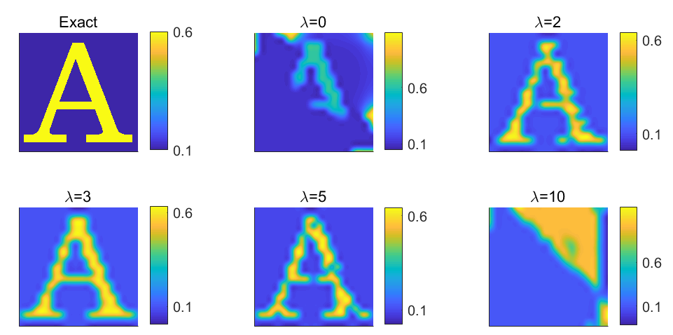
Figure 1: Test 1. The reconstructed results of function $\beta(\mathbf{x})$ with different $\lambda$ in (5.4). The function $\beta(\mathbf{x})$ is given in (8.7) with $c_{\beta}=0.6$ inside of the letter ‘A’ and the function $\gamma(\mathbf{x})$ is given in (8.8) with $c_{\gamma}=0.4$ inside of the letter ‘$\Omega$’.

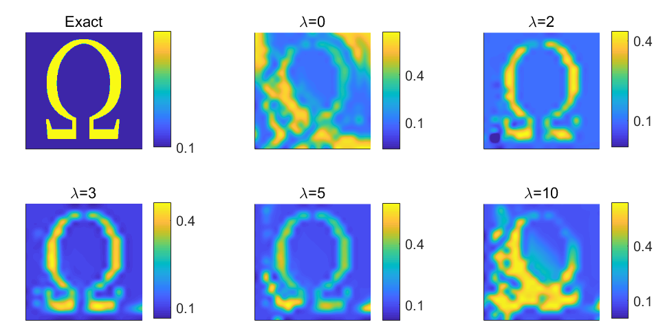
Figure 2: Test 1. The reconstructed results of function $\gamma(\mathbf{x})$ with different $\lambda$ in (5.4). The function $\beta(\mathbf{x})$ is given in (8.7) with $c_{\beta}=0.6$ inside of the letter ‘A’ and the function $\gamma(\mathbf{x})$ is given in (8.8) with $c_{\gamma}=0.4$ inside of the letter ‘$\Omega$’. Thus, it is clear from Figure 1 and Figure 2 that the presence of the CWF in the functional $J_{\lambda,\xi}\left(W\right)$ is necessary since the images for $\lambda=0$ are poor. It is also clear that $\lambda=3$ is the optimal value of the parameter $\lambda$.

Using the solution of the Minimization Problem, we can reconstruct the functions $\rho_{S},\rho_{I},\rho_{R}$ via (3.5). At $t=0.75$, the solutions of the forward problem (2.2)-(2.6) with known coefficient functions $\beta(\mathbf{x})$ and $\gamma(\mathbf{x})$ are indicated by ‘Exact’, and the reconstructed functions $\rho_{S},\rho_{I},\rho_{R}$ by (3.5) are indicated by ‘Reconstructed’ in Figure 3. The reconstructed functions $\rho_{S},\rho_{I},\rho_{R}$ are almost as same as the solutions of the forward problem. In other words, solving our Coefficient Inverse Problem (2.9), (2.10) we can accurately calculate the values of functions $\rho_{S}\left(\mathbf{x},t\right),\rho_{I}\left(\mathbf{x},t\right)$ and $\rho_{R}\left(\mathbf{x},t\right)$ for $\left(\mathbf{x},t\right)\in Q_{T}.$

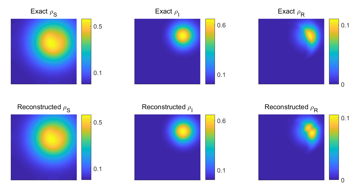
Figure 3: Test 1. The exact (top line) and reconstructed (bottom line) functions $\rho_{S}$ (left column), $\rho_{I}$ (middle line) and $\rho_{R}$ (right line) at $t=0.75$, where the function $\beta(\mathbf{x})$ is given in (8.7) with $c_{\beta}=0.6$ inside of the letter ‘A’ and the function $\gamma(\mathbf{x})$ is given in (8.8) with $c_{\gamma}=0.4$ inside of the letter ‘$\Omega$’.

Test 2. We test the case when the inclusion of $\beta(\mathbf{x})$ in (8.7) has the shape of the letter ‘$B$’ with $c_{\beta}=0.4$ and the inclusion of $\gamma(\mathbf{x})$ in (8.8) has the shape of the letter ‘$D$’ with $c_{\gamma}=0.6$. The result is displayed in Figure 4.

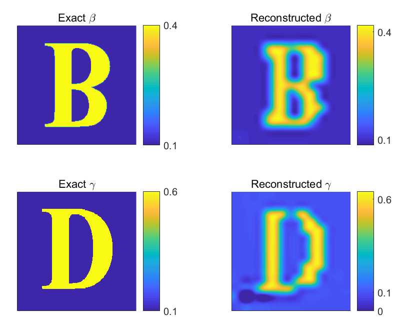
Figure 4: Test 2. The exact (left) and reconstructed (right) functions $\beta(\mathbf{x})$ (top line) and $\gamma(\mathbf{x})$ (bottom line), where the function $\beta(\mathbf{x})$ is given in (8.7) with $c_{\beta}=0.4$ inside of the letter ‘B’ and the function $\gamma(\mathbf{x})$ is given in (8.8) with $c_{\gamma}=0.6$ inside of the letter ‘D’.

Test 3. Following Test 1, the noisy data is considered. The result is displayed in Figure 5.

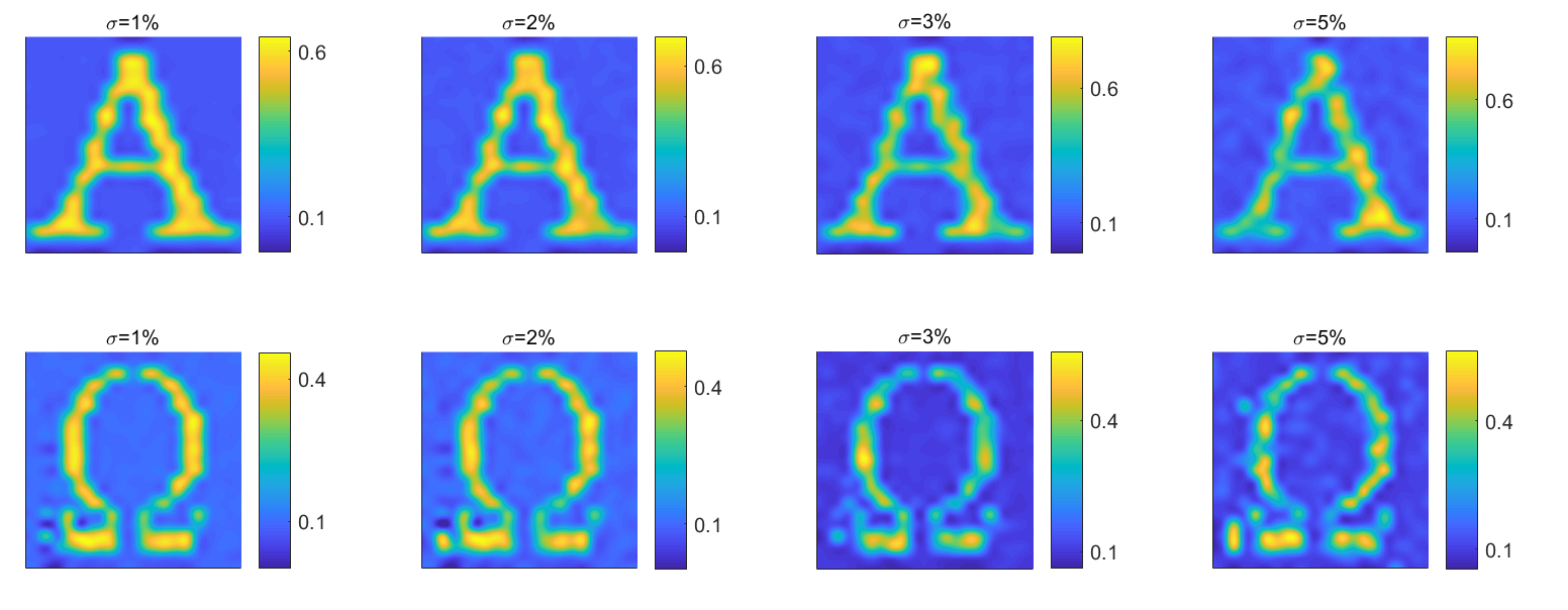
Figure 5: Test 3. The reconstructed functions $\beta(\mathbf{x})$ (top line) and $\gamma(\mathbf{x})$ (bottom line) with $\sigma=0.01$ (1st column), $\sigma=0.02$ (2ed column), $\sigma=0.03$ (3rd column) and $\sigma=0.05$ (4th column).

9 Summary

This is the first work,  in which a Coefficient Inverse Problem for the spatiotemporal SIR model of [26] is considered. We have constructed a new version of the convexification method for this CIP. The main conclusion of our convergence analysis is the global convergence of this method. In other words, its convergence to the true solution is guaranteed regardless on the availability of a good initial guess. The key to the global convergence property is the presence of the Carleman Weight Function in the resulting Tikhonov-like regularization functional, and this is clearly confirmed in the numerical Test 1, see Figure 1 and Figure 2. As a by-product, uniqueness theorem for our CIP is proven.

Results of our numerical studies demonstrate an accurate performance of our method for rather complicated shapes of abnormalities. Since the minimal amount of measured data are required in our CIP, then results of this paper indicate a possibility of a significant decrease of the cost of the spatiotemporal monitoring of the spread of epidemics in affected cities.

References

• [1] M. Asadzadeh and L. Beilina, Stability and convergence analysis of a domain decomposition FE/FD method for Maxwell’s equations in the time domain, Algorithms 15 (2022), 337.
• [2] M. Asadzadeh and L. Beilina, A stabilized P1 domain decomposition finite element method for time harmonic Maxwell’s equations, Math. Comput. Simul 204 (2023), 556–574.
• [3] A. B. Bakushinskii, M. V. Klibanov, and N. A. Koshev, Carleman weight functions for a globally convergent numerical method for ill-posed Cauchy problems for some quasilinear PDEs, Nonlinear Analysis: Real World Applications 34 (2017), 201–224.
• [4] L. Baudouin, M. de Buhan, E. Crépeau, and J. Valein, Carleman-based reconstruction algorithm on a wave network, HAL (Le Centre pour la Communication Scientifique Directe), available online, https://hal.science/hal-04361363 (2023).
• [5] L. Baudouin, M. de Buhan, and S. Ervedoza, Convergent algorithm based on Carleman estimates for the recovery of a potential in the wave equation, SIAM J. Numer. Anal. 55 (2017), 1578–1613.
• [6] L. Baudouin, M. de Buhan, S. Ervedoza, and A. Osses, Carleman-based reconstruction algorithm for the waves, SIAM J. Numer. Anal. 59 (2021), 998–1039.
• [7] L. Beilina, M. G. Aram, and E. M. Karchevskii, An adaptive finite element method for solving 3D electromagnetic volume integral equation with applications in microwave thermometry, J. Comput. Phys. 459 (2022), 111122.
• [8] L. Beilina and V. Ruas, On the Maxwell-wave equation coupling problem and its explicit finite-element solution, Appl. Math. 68 (2022), 75–98.
• [9] A. L. Bukhgeim and M. V. Klibanov, Uniqueness in the large of a class of multidimensional inverse problems, Soviet Math. Doklady 17 (1981), 244–247.
• [10] G. Chavent, Nonlinear least squares for inverse problems: Theoretical foundations and step-by-step guide for applications, Springer Science & Business Media, New York, 2009.
• [11] A. V. Goncharsky and S. Y. Romanov, Iterative methods for solving coefficient inverse problems of wave tomography in models with attenuation, Inverse Probl. 33 (2017), 025003.
• [12] A. V. Goncharsky and S. Y. Romanov, A method of solving the coefficient inverse problems of wave tomography, Comput. Math. Appl. 77 (2019), 967–980.
• [13] W. O. Kermack and A. G. McKendrick, A contribution to the mathematical theory of epidemics, Proc. Roy. Soc. London Ser. A 115 (1927), no. 772, 700–721.
• [14] M. V. Klibanov, Inverse problems and Carleman estimates, Inverse Probl. 8 (1992), 575–596.
• [15] M. V. Klibanov, Global convexity in a three-dimensional inverse acoustic problem, SIAM J. Math. Anal. 28 (1997), 1371–1388.
• [16] M. V. Klibanov, Carleman estimates for global uniqueness, stability and numerical methods for coefficient inverse problems, J. Inverse Ill-Posed Probl. 21 (2013), 477–510.
• [17] M. V. Klibanov and O. V. Ioussoupova, Uniform strict convexity of a cost functional for three-dimensional inverse scattering problem, SIAM J. Math. Anal. 26 (1995), 147–179.
• [18] M. V. Klibanov, V. A. Khoa, A. V. Smirnov, L. H. Nguyen, G. W. Bidney, L. Nguyen, A. Sullivan, and V. N. Astratov, Convexification inversion method for nonlinear SAR imaging with experimentally collected data, J. Appl. Ind. Math. 15 (2021), 413–436.
• [19] M. V. Klibanov and J. Li, Inverse problems and Carleman estimates: Global uniqueness, global convergence and experimental data, De Gruyter, Berlin, 2021.
• [20] M. V. Klibanov, J. Li, L. Nguyen, and Z. Yang, Convexification numerical method for a coefficient inverse problem for the radiative transport equation, SIAM J. Imag. Sci. 16 (2023), no. 1, 35–63.
• [21] M. V. Klibanov, J. Li, L. H. Nguyen, V. G. Romanov, and Z. Yang, Convexification numerical method for a coefficient inverse problem for the Riemannian radiative transfer equation, SIAM J. Imag. Sci. 16 (2023), 1762–1790.
• [22] M. V. Klibanov, J. Li, and Z. Yang, Convexification for a coefficient inverse problem of mean field games, arXiv:2310.08878 (2023).
• [23] M.V. Klibanov, J. Li, and W. Zhang, Convexification for an inverse parabolic problem, Inverse Probl. 36 (2020), 085008.
• [24] O. A. Ladyzhenskaya, V. A. Solonnikov, and N. N. Uralceva, Linear and quasilinear equations of parabolic type, vol. 23, AMS, Providence, R.I., 1968.
• [25] M. M. Lavrentiev, V. G. Romanov, and S. P. Shishatskii, Ill-Posed Problems of Mathematical Physics and Analysis, AMS, Providence, R. I., 1986.
• [26] W. Lee, S. Liu, H. Tembine, W. Li, and S. Osher, Controlling propagation of epidemics via mean-field control, SIAM J. Appl. Math. 81 (2021), no. 1, 190–207.
• [27] L. H. Nguyen, The Carleman contraction mapping method for quasilinear elliptic equations with over-determined boundary data, Acta Mathematica Vietnamica 48 (2023), no. 3, 401–422.
• [28] L. H. Nguyen and M. V. Klibanov, Carleman estimates and the contraction principle for an inverse source problem for nonlinear hyperbolic equations, Inverse Probl. 38 (2022), no. 3, 035009.
• [29] R. G. Novikov, The inverse scattering problem on a fixed energy level for the two-dimensional Schrödinger operator, J. Funct. Anal. 103 (1992), no. 2, 409–463.
• [30] R. G. Novikov, The $\bar{\partial}-$approach to approximate inverse scattering at fixed energy in three dimensions, International Math. Research Peports 6 (2005), 287–349.
• [31] V. G. Romanov, Inverse problems of mathematical physics, VNU Press, Utrecht, The Netherlands, 1986.
• [32] J. A. Scales, M. L. Smith, and T. L. Fischer, Global optimization methods for multimodal inverse problems, J. Comp. Phys. 103 (1992), 258–268.
• [33] A. N. Tikhonov, A. V. Goncharsky, V. V. Stepanov, and A. G. Yagola, Numerical methods for the solution of Ill-posed problems, Kluwer, London, 1995.
• [34] M. M. Vajnberg, Variational method and method of monotone operators in the theory of nonlinear equations, Israel Program for Scientific Translations, Jerusalem-London, 1973.
• [35] M. Yamamoto, Carleman estimates for parabolic equations, Topical Review. Inverse Probl. 25 (2009), 123013.