Intersection Numbers, Polynomial Division and Relative Cohomology

Abstract

We present a simplification of the recursive algorithm for the evaluation of intersection numbers for differential $n$-forms, by combining the advantages emerging from the choice of delta-forms as generators of relative twisted cohomology groups and the polynomial division technique, recently proposed in the literature. We show that delta-forms capture the leading behaviour of the intersection numbers in presence of evanescent analytic regulators, whose use is, therefore, bypassed. This simplified algorithm is applied to derive the complete decomposition of two-loop planar and non-planar Feynman integrals in terms of a master integral basis. More generally, it can be applied to derive relations among twisted period integrals, relevant for physics and mathematical studies.

1 Introduction

The intersection number between differential $n$-forms matsumoto1994 ; matsumoto1998 ; OST2003 ; doi:10.1142/S0129167X13500948 ; goto2015 ; goto2015b ; Yoshiaki-GOTO2015203 ; Mizera:2017rqa ; matsubaraheo2019algorithm ; Ohara98intersectionnumbers ; https://doi.org/10.48550/arxiv.2006.07848 ; https://doi.org/10.48550/arxiv.2008.03176 ; https://doi.org/10.48550/arxiv.2104.12584 is an elementary quantity that rules the vector space properties of regulated (twisted period) integrals. The respective integrands are defined through the product of the twist, a regulating multivalued function that vanishes at the boundary of the integration domain, and a differential $n$-form. Acting as an inner product, the intersection number yields the decomposition of the differential forms into a basis of forms that generate the twisted de Rham cohomology group, a vector space defined as the quotient space of the closed forms modulo the exact forms Mastrolia:2018uzb ; Frellesvig:2019kgj ; Frellesvig:2019uqt ; Frellesvig:2020qot . Linear and quadratic relations among the elements of the vector space, as well as differential and difference equations for them, can be derived using intersection numbers. The translation of these identities to their respective integral formulations is then straightforward.

The algebraic properties of Feynman integrals, central objects of study in perturbative classical and quantum field theory, motivated us to develop the intersection theory framework. In that framework the linear relations derived by intersection numbers are equivalent to the well-known integration-by-parts identities (IBPs) Tkachov:1981wb ; Chetyrkin:1981qh , used to derive the integrals decomposition in terms of an independent set of master integrals (MIs), as well as for the differential and difference equations obeyed by them. The same formalism can be applied to a wider class of functions, such as Aomoto-Gelfand and Euler-Mellin integrals, as well as Gelfand-Kapranov-Zelevinsky hypergeometric systems GKZ-1989 ; GKZ-Euler-1990 ; Chestnov:2022alh which embed Feynman integrals as special restrictions Chestnov:2023kww (see also Agostini:2022cgv ; Matsubara-Heo:2023ylc ). Beyond IBP reductions, twisted co-homology finds applications in many other relevant areas of Physics and Mathematics: the formalism has been applied in the construction of the canonical bases for Feynman integrals Chen:2020uyk ; Chen:2022lzr ; Chen:2023kgw ; Giroux:2022wav (in presence of generalised polylogarithms as well as of elliptic functions), correlator functions in quantum field theory and lattice gauge theory Weinzierl:2020gda ; Weinzierl:2020nhw ; Cacciatori:2022mbi ; Gasparotto:2022mmp ; Gasparotto:2023roh (in perturbative and non-perturbative approaches), orthogonal polynomials, quantum mechanical matrix elements, Witten-Kontsevich tau-functions Cacciatori:2022mbi , cosmological correlators De:2023xue , representation of Feynman integrals as single-valued hypergeometric functions Duhr:2023bku , to name a few.

There exist several methods for the calculation of intersection numbers using the twisted version of Stokes’ theorem cho1995 . In the special case of logarithmic $n$-forms they can be computed via the algorithms proposed in matsumoto1998 ; Mizera:2017rqa ; Mizera:2019vvs ; Matsubara-Heo:2021dtm . In the more general situation of meromorphic $n$-forms, the calculation of the intersection number can proceed according to the so-called recursive approach, as proposed in Mizera:2019gea ; Frellesvig:2019uqt ; Frellesvig:2020qot , elaborating on Ohara98intersectionnumbers , which, exploiting the concept of fibration, maps the (evaluation of) intersection numbers for $n$-forms, into an ordered sequence of (evaluations of) intersection numbers for 1-forms, that are computed by considering one (integration) variable at a time. This method can be simplified by exploiting the invariance of the representative of the cohomology classes and by avoiding the use of algebraic extensions Weinzierl:2020xyy , and its application range can be extended Caron-Huot:2021xqj ; Caron-Huot:2021iev also to the case of the relative twisted cohomology matsumoto2018relative , that deals with singularities of the integrand not regulated by the twist. An interesting improvement of the evaluation procedure, that makes use of the idea of avoiding polynomial factorisation and algebraic extensions, has been recently proposed in Fontana:2023amt , by introducing the polynomial series expansion technique, and an efficient treatment of the analytic regulators, combined with the advantages of modular arithmetic over the finite fields Peraro:2016wsq ; Peraro:2019svx .

Also, we have recently proposed a new algorithm for computing the intersection number of twisted $n$-forms, based on a multivariate version of Stokes’ theorem, which requires the solution of a higher-order partial differential equation and the evaluation of multivariate residues Chestnov:2022xsy , which is a natural generalization of the original algorithm cho1995 ; matsumoto1998 that avoids the fibration procedure.

Let us finally mention that an alternative method for evaluation of intersection numbers, which is based on the solution of the secondary equation built from the Pfaffian system of differential equations for the generators of the cohomology group Matsubara-Heo-Takayama-2020b ; matsubaraheo2019algorithm , in combination with an efficient algorithm for construction of such systems by means of the Macaulay matrix has recently been proposed in Chestnov:2022alh .

The previous activities show that the development of the optimal algorithms for evaluating intersection numbers for meromorphic twisted $n$-forms is an open problem of common interest for mathematicians and physicists.

The classification of dimensionally regulated Feynman integrals as twisted period integrals becomes manifest when, instead of the canonical momentum-space representation, parametric representations of the integrals are adopted Lee:2013hzt ; Mastrolia:2018uzb . Additional analytic regularisation Speer:1969sjv ; Speer1971 is often required to regulate the behaviour of inverse powers of the integration variables that arise upon the change of variables, from the loop momenta to the new set of $n$ integration variables. Accordingly, auxiliary non-integer regulating exponents, hereby dubbed ${\it regulators}$, are introduced in the definition of the twist Frellesvig:2017aai , which are later set to zero at the end of the calculation of the coefficients of the MIs decomposition. Therefore, intersection numbers acquire a dependence on the evanescent regulators, beside the expected dependence on external kinematic invariants, masses, and the continuous space-time dimensions $d$. For that reason the regulators affect the load of the evaluation algorithm, which would be much lighter if they were absent.

In the case of Euler-Mellin integrals and GKZ hypergeometric functions, non-integer exponents are considered ab-initio in the integral representation, and, in these cases, the intersection numbers depend on them, as well as on the multiplicative factors of the monomials (product of integration variables) that appear in the twist - which can be considered as external variables.

In this work, we investigate the analytic behaviour of the intersection numbers of 1-forms on one evanescent regulator, and show that the coefficients of the MIs decomposition can be computed just using the leading term (LT) of the Laurent series expansion of the intersection numbers, as it was remarkably observed, by other means, in Fontana:2023amt . Moreover, we show that the expression of the LT of the expansion is equivalent to the result of the intersection number computed within the relative twisted cohomology theory matsumoto2018relative , obtained by means of the delta-forms introduced in Caron-Huot:2021xqj ; Caron-Huot:2021iev . Although derived in the case of 1-form, the result of our analysis allows us to present an simplification of the recursive algorithm for the evaluation of intersection numbers of twisted $n$-forms, and to apply it to the complete decomposition of a few non-trivial representative types of Feynman integrals at one and two loops, with planar and non-planar configurations, in terms of bases of MIs. On the one hand, we adapt the polynomial expansion technique introduced in Fontana:2023amt , by proposing a novel choice of the polynomial-ideal generator in the intermediate layers of the recursive approach. On the other hand, we eliminate the need for the analytic regulators, by applying the relative twisted cohomology theory matsumoto2018relative ; Caron-Huot:2021xqj ; Caron-Huot:2021iev , and present a systematic algorithm for choosing multivariate delta-forms as elements of the dual cohomology bases, to significantly simplify the computation of the intersection numbers.

The chosen examples of Feynman integrals involve differential $n$-forms with $n$ up to nine. The intersection-theory based decomposition is performed on cuts, along the lines of Frellesvig:2019kgj ; Frellesvig:2020qot , so that the determination of the coefficients of the integral decomposition require intersection numbers of $n$-forms, with $n$ up to six, only. In particular, we describe in detail the decomposition via intersection numbers of integrals related to the one-loop box diagram contributing to Bhabha scattering, as well as the planar and non-planar massless double-box diagrams. Computational details for the latter two cases can be found in the ancillary files Dbox_massless.m and Dbox_massless_nonplanar.m, respectively. For the decomposition of the integrals related to the planar and non-planar double-box diagrams with one massive external leg, in the text we provide just the bases of $n$-forms and give the computational details, respectively, in the ancillary files Dbox_1m.m, and Dbox_1m_nonplanar.m. The decomposition formulas are found to be equivalent to the results of an IBP decomposition. These results demonstrate that, using intersection numbers it is possible to obtain the direct and complete decomposition of non-trivial integrals in terms of MIs, just like any generic element of a vector space can be projected onto a set of generators.

This work is organized as follows: In Section 2 a review of the twisted de Rham cohomology and intersection numbers is given. Section 3 contains a discussion of the application of polynomial division and global residues for the efficient computation of intersection numbers. Section 4 describes the computation of intersection numbers within the relative twisted cohomology theory using delta-forms, as well as their derivation as limits of cases with analytic regulators within the regular twisted cohomology theory. Applications to the decomposition of one- and two-loop Feynman integrals are presented in Section 5 to showcase the novel techniques introduced in this work. We provide concluding remarks in Section 6.

The manuscript contains two appendices: Appendix A contains a description of the extended euclidean algorithm and Appendix B contains an example of our algorithm for building the bases for the (relative) twisted cohomology groups.

For our research, the following software has been used: LiteRed Lee:2012cn ; Lee:2013mka , Fire Smirnov:2019qkx , FiniteFlow Peraro:2019svx , Fermat Fermat , Fermatica Fermatica , Mathematica, HomotopyContinuation HomotopyContinuation.jl , Singular DGPS and its Mathematica interface Singular.m SingularInterface , and Jaxodraw Binosi:2008ig ; Axodraw:1994 .

2 Integrals and Twisted Cohomology Groups

In this section we review some basic properties of twisted cohomology and intersection theory, focusing on the evaluation of intersection numbers for $1$- and $n$-forms.

The frameworks of twisted homology and cohomology are concerned with twisted period integrals of the form

$$I =\int_{\mathcal{C}_{R}}\!u\ \varphi_{L}:=\langle\varphi_{L}|\mathcal{C}_{R}]\>,$$ (1)

where $\varphi_{L}$ is a rational/meromorphic $n$-form: $\varphi_{L}={\widehat{\varphi}}_{L}(z)\,\mathrm{d}\mathbf{z}\equiv{\widehat{\varphi}}_{L}(z)\,\mathrm{d}z_{1}\wedge\ldots\wedge\mathrm{d}z_{n}$, and $u$ is a multivalued function

$$u=\prod_{i}B_{i}^{\gamma_{i}}\>,$$ (2)

called the twist, with generic (polynomial) factors $B_{i}=B_{i}(z)$ and generic exponents $\gamma_{i}\>$. The generiticity condition on the $\gamma_{i}$ is required to ensure that all poles of $\varphi_{L}$ are regulated by $u$. Moreover, the integration domain ${\cal C}$ is chosen such that $B_{i}(\partial{\cal C})=0$. The latter condition ensures that twisted period integrals obey integration-by-part identities (IBPs)

$$\int_{\mathcal{C}_{R}}\!\mathrm{d}(u\,\phi_{L})=0\>,$$ (3)

corresponding to the vanishing integrals

$$\int_{\mathcal{C}_{R}}\!u\,\nabla_{\omega}\,\phi_{L}=\langle\nabla_{\omega}\,\phi_{L}|\mathcal{C}_{R}]=0\>,$$ (4)

where we introduced the covariant derivative $\nabla_{\omega}\>$, defined as,

$$\nabla_{\omega}:=\mathrm{d}+\omega\>,\qquad\text{with}\;\;\qquad\omega:=\mathrm{d}\log(u)=\sum_{i=1}^{n}\widehat{\omega}_{i}\,\mathrm{d}z_{i}\>,\qquad\text{and}\;\;\qquad\widehat{\omega}_{i}:=\partial_{z_{i}}\log(u)\>.$$ (5)

Within twisted de Rham theory, any $n$-form $\varphi_{L}$ is a member (equivalence class representative) of the vector space of closed modulo exact $n$-forms, called the $n$^th twisted cohomology group $\mathrm{H}^{n}_{\omega}\>$. The equivalence relation reads $\langle\varphi_{L}|\sim\langle\varphi_{L}+\nabla_{\omega}\phi_{L}|$, where $\phi_{L}$ is a generic $(n{-}1)$-form. $\mathrm{H}^{n}_{\omega}$ identifies integrands that give the same $I$, upon integration over ${\cal C}_{R}\>$. The number $\nu:=\mathrm{dim}\left(\mathrm{H}_{\omega}^{n}\right)$ of independent equivalence classes is the dimensionality of the cohomology group.

We may also introduce the dual integrals:

$$I^{\vee} =\int_{\mathcal{C}_{L}}\!u^{-1}\ \varphi_{R}:=[\mathcal{C}_{L}|\varphi_{R}\rangle\>,$$ (6)

whose integrands contains the multivalued function $u^{-1}$ and the dual $n$-form $\varphi_{R}\>$. Similarly to the previous case, $|\varphi_{R}\rangle\sim|\varphi_{R}+\nabla_{-\omega}\phi_{R}\rangle$ with $\phi_{R}$ being an $(n{-}1)$-form. Thus $\varphi_{R}$ is a member of another vector space of closed modulo exact $n$-forms, called the $n$^th dual twisted cohomology group $\mathrm{H}^{n}_{-\omega}\>$. Elements of this group identify integrands that give the same $I^{\vee}$, upon integration over ${\cal C}_{L}\>$.

Stokes’ theorem motivates the examination of the equivalence classes of integration domains ${\cal C}_{L,R}$ (called the $n$^th twisted chains), which form the other two vector spaces $\mathrm{H}_{n}^{\pm\omega}$ referred to as the (dual) twisted $n$^th homology groups. In turn, de Rham’s theorem ensures that the four vector spaces $\mathrm{H}^{n}_{\pm\omega}$ and $\mathrm{H}_{n}^{\pm\omega}$ are isomorphic, which implies that $\mathrm{dim}\left(\mathrm{H}_{\omega}^{n}\right)=\mathrm{dim}\left(\mathrm{H}_{-\omega}^{n}\right)=$ $\mathrm{dim}\left(\mathrm{H}^{\omega}_{n}\right)=\mathrm{dim}\left(\mathrm{H}^{-\omega}_{n}\right)$.

In the case of Feynman integrals, the dimension of the twisted cohomology group corresponds to the number of master integrals:

$$\nu =\mathrm{dim}\left(\mathrm{H}^{n}_{\pm\omega}\right)=\mathrm{dim}\left(\mathrm{H}_{n}^{\pm\omega}\right)$$

$$=\text{number of zeros of $\omega$}\>,$$ (7)

which is determined by the number of critical points of the Morse height function $\log(|u|)$ Lee:2013hzt .

Let us consider the bases $\{\langle e_{i}|\}_{i=1,\cdots,\nu}$ belonging to $\mathrm{H}^{n}_{\omega}$ and the dual bases $\{|h_{i}\rangle\}_{i=1,\cdots,\nu}$ belonging to $\mathrm{H}^{n}_{-\omega}$. Then any arbitrary cocycle ($\langle\varphi_{L}|$) can be decomposed in terms of these bases following the master decomposition formula Mastrolia:2018uzb ; Frellesvig:2019kgj . This relation expresses a given cocycle $\langle\varphi_{L}|$ in terms of a given basis $\langle{e}_{i}|$:

$$\langle\varphi_{L}|=\sum_{i=1}^{\nu}c_{i}\langle{e}_{i}|\>,\qquad\quad\text{with}\qquad\quad c_{i}=\langle{\varphi_{L}}\,|\,{h}_{j}\rangle({\bf C}^{-1})_{ji}\>,$$ (8)

where the square matrix of all possible intersection numbers between the left- and right-bases

$${\bf C}_{ij}:=\langle{e}_{i}\,|\,{h}_{j}\rangle$$ (9)

is called the metric or simply the ${\bf C}$-matrix.

Following the master decomposition formula Mastrolia:2018uzb ; Frellesvig:2019kgj , any Feynman integral $I$ can be decomposed in terms of the master integrals $J_{i}$ as

$$I=\langle\varphi_{L}|\mathcal{C}]\ =\sum_{i=1}^{\nu}c_{i}\langle e_{i}|\mathcal{C}]=\sum_{i=1}^{\nu}c_{i}\,J_{i}\,,$$ (10)

where the coefficients of the decomposition $c_{i}$ are given by eq. (8) and $J_{i}=\langle e_{i}|\mathcal{C}\big{]}$ . Let us observe that $c_{i}$ is independent of the choice of the dual bases $|h_{j}\rangle$ Frellesvig:2019kgj , and that, this degree of freedom can be exploited to simplify the computing algorithm - as it soon will be made clear.

2.1 Intersection numbers for $1$-forms

The intersection number is an integral of the product between the left and right forms. To define it consistently, one of the forms has to be regulated by expressing it as a specific representative of its cohomology class:

$$\langle\varphi_{L}\,|\,\varphi_{R}\rangle:=\frac{1}{2\pi i}\int_{\mathcal{X}}\!\iota(\varphi_{L})\wedge\varphi_{R}=-\frac{1}{2\pi i}\int_{\mathcal{X}}\!\varphi_{L}\wedge\iota(\varphi_{R})\>,$$ (11)

where the $\iota$-operator denotes the regularization procedure defined in the univariate case as:

$$\iota(\varphi_{L}):=\varphi_{L}-\nabla_{\!\omega}(h\psi_{L})\>,\qquad\iota(\varphi_{R}):=\varphi_{R}-\nabla_{\!-\omega}(h\psi_{R})\>,$$ (12)

with the Heaviside functions

$$h:=\sum_{i\in\mathcal{P}_{\omega}}(1-\theta_{z,i})\>,\qquad\theta_{z,i}:=\theta(|z{-}z_{i}|-\epsilon)\>,\qquad\mathcal{P}_{\omega}:=\bigl{\{}\text{poles of $\omega$}\bigr{\}}\>.$$ (13)

The domain of integration in eq. (11) is defined as $\mathcal{X}:=\mathbb{C}\mathrm{P}\setminus\mathcal{P}_{\omega}\>$, and the set of singularities $\mathcal{P}_{\omega}$ includes also $z=\infty$. The functions $\psi_{L}$ and $\psi_{R}$ are the solutions to the differential equations:

$$\nabla_{\!\omega}\psi_{L}=\varphi_{L}\>,\qquad\nabla_{\!-\omega}\psi_{R}=\varphi_{R}\>.$$ (14)

To compute intersection numbers eq. (14) must be solved around each pole $p\in\mathcal{P}_{\omega}\>$. Considering the pole at $z=p$, the solution around this pole formally reads matsumoto1998 ; matsumoto2018relative ,

$$\psi_{L,p}(z) =\frac{1}{(\eta_{+}-1)\,u(z)}\int_{C_{p}(z)}\!\!u(t)\,\varphi_{L}(t)\>,$$ (15)

$$\psi_{R,p}(z) =\frac{u(z)}{(\eta_{-}-1)}\int_{C_{p}(z)}\!\!\frac{\varphi_{R}(t)}{u(t)}\>.$$

Here $C_{p}(z)$ is the contour given in Figure 1 and $\eta_{\pm}=e^{\pm 2\pi i\alpha_{p}}$, with $\alpha_{p}$ being the non-integer exponent of $u$ at $z=p$ (and thus $-\alpha_{p}$ the exponent of $u^{-1}$).

Figure 1: The integration contour $C_{p}(z)$ used in eq. (15).

Following Mastrolia:2018uzb ; Frellesvig:2019kgj we may then derive the expression for the univariate intersection number as

$$\langle\varphi_{L}\,|\,\varphi_{R}\rangle=\sum_{p\in\mathcal{P}_{\omega}}{\rm Res}_{z=p}(\psi_{L,p}\,\varphi_{R})=-\sum_{p\in\mathcal{P}_{\omega}}{\rm Res}_{z=p}(\psi_{R,p}\,\varphi_{L})\>.$$ (16)

2.2 Intersection numbers for $n$-forms

The intersection number for $n$-forms can be computed by adopting more than one computational strategy. In this work, we will use the fibration-based approach discussed in Frellesvig:2019uqt ; Frellesvig:2020qot , which can be applied to generic meromorphic forms. This method treats the integration variables one at a time, so, without loss of generality, we may order them as $z_{n},\ldots,z_{1}$, listed from the outer to the innermost integration. Each layer of the fibration has its own (internal) basis of master forms, whose size can be counted using eq. (7), and can be efficiently chosen following the algorithm explained in Section 4.4 and Appendix B. We denote such bases of forms and their duals on the $m^{\text{th}}$ layer by $e^{(\mathbf{m})}_{i}$ and $h^{(\mathbf{m})}_{i}$ respectively, and their dimension by $\nu_{m}$.

This approach allows us to compute multivariate intersection numbers recursively: Assuming all the $(m-1)$-variate building blocks are known, the $m$-variable intersection numbers can be evaluated using

$$\langle\varphi^{{(\mathbf{m})}}_{L}\,|\,\varphi^{{(\mathbf{m})}}_{R}\rangle=\sum_{p\in\mathcal{P}^{(m)}}\!\!{\rm Res}_{z_{m}=p}\left(\psi_{L,i}^{(m)}{\bf C}^{(m-1)}_{ij}{\varphi_{R,j}^{(m)}}\right)=\sum_{p\in\mathcal{P}^{(m)}}\!\!{\rm Res}_{z_{m}=p}\left(\psi_{L,i}^{(m)}\langle e^{(\mathbf{m-1})}_{i}\,|\,\varphi^{{(\mathbf{m})}}_{R}\rangle\right)\>,$$ (17)

where the ${\bf C}$-matrix and the projections are given by

$${\bf C}^{(m)}_{ij} :=\langle e^{(\mathbf{m})}_{i}\,|\,h^{(\mathbf{m})}_{j}\rangle\>,$$ (18)

$$\varphi^{(m)}_{L,i} =\sum_{j=1}^{\nu_{m-1}}\langle\varphi^{{(\mathbf{m})}}_{L}\,|\,h^{(\mathbf{m-1})}_{j}\rangle\,({\bf C}_{(m-1)}^{-1})_{ji}\>,$$ (19)

$$\varphi^{(m)}_{R,i} =\sum_{j=1}^{\nu_{m-1}}({\bf C}_{(m-1)}^{-1})_{ij}\,\langle e^{(\mathbf{m-1})}_{j}\,|\,\varphi^{{(\mathbf{m})}}_{R}\rangle\>.$$ (20)

The key formula (17) relies on the solution to the system of differential equations:

$$\Bigl{[}\delta_{ij}\partial_{z_{m}}+\Omega^{(m)}_{ji}\Bigr{]}\,\psi_{L,j}^{(m)}=\varphi_{L,i}^{(m)}\>,\quad\;\;\text{where}\quad\;\;\Omega^{(m)}_{ij}=\langle(\partial_{z_{m}}{+}\omega_{m})e^{(\mathbf{m-1})}_{i}\,|\,h^{(\mathbf{m-1})}_{k}\rangle\,\bigl{(}{\bf C}_{(m-1)}^{-1}\bigr{)}_{kj}\,.$$ (21)

The $\Omega^{(m)}$ matrix also known as the connection matrix defines the set of singularities $\mathcal{P}^{(m)}$ appearing in eq. (17) as

$$\mathcal{P}^{(m)}:=\bigl{\{}\text{poles of $\Omega^{(m)}$}\bigr{\}}\>,$$ (22)

which also includes $z=\infty$. In complete analogy to the univariate case of Section 2.1, we may write the dual representation of eq. (17) as

$$\langle\varphi^{{(\mathbf{m})}}_{L}\,|\,\varphi^{{(\mathbf{m})}}_{R}\rangle=-\sum_{p\in\mathcal{P}^{(m)}}\!\!{\rm Res}_{z_{m}=p}\Bigl{(}{\varphi_{L,i}^{(m)}}{\bf C}^{(m-1)}_{ij}\psi_{R,j}^{(m)}\Bigr{)}=-\sum_{p\in\mathcal{P}^{(m)}}\!\!{\rm Res}_{z_{m}=p}\Bigl{(}\langle\varphi^{{(\mathbf{m})}}_{L}|h^{(\mathbf{m-1})}_{i}\rangle\,\psi_{R,i}^{(m)}\Bigr{)}\,,$$ (23)

which makes use of the solution $\psi_{R}$ to the dual differential equation and the dual connection $\Omega^{\vee(m)}$ given by

$$\Bigl{[}\delta_{ij}\partial_{z_{m}}+\Omega^{\vee(m)}_{ij}\Bigr{]}\,\psi_{R,j}^{(m)}=\varphi_{R,i}^{(m)}\>,\quad\text{where}\quad\;\Omega^{\vee(m)}_{ij}=\bigl{(}{\bf C}_{(m-1)}^{-1}\bigr{)}_{ik}\,\langle e^{(\mathbf{m-1})}_{k}\,|\,(\partial_{z_{m}}{-}\omega_{m})h^{(\mathbf{m-1})}_{j}\rangle\>.$$ (24)

3 Intersection Numbers and Polynomial Division

In general, the evaluation of intersection numbers in eqs. (11, 17) requires the solution of the differential equations (14, 21), and a residue operation. In the univariate case, these operations are performed locally around each pole of the function $\omega$ defined in eq. (5), and likewise with the poles of $\Omega$ in the multivariate case. Individual contributions to the intersection number from each pole may contain irrational terms, which only cancel upon considering their sum. In this section we recall the idea proposed in Fontana:2023amt to show how intersection numbers can be computed bypassing the precise identification of singularities of $\omega$, thus avoiding algebraic extensions: polynomial division and global residues can be used to derive the solution of the differential equation, and to extract the sum over local residues directly from the remainders of iterated polynomial divisions. In the application of these techniques, within the recursive algorithm for the evaluation of intersection numbers, we propose the use of a novel polynomial, built as the least common multiple of the denominators appearing in the connection matrix.

3.1 Polynomial decomposition and global residue

Univariate polynomials

The decomposition of a univariate polynomial $p(z)$ in terms of another degree $\kappa$ polynomial $B(z)$ may be written as

$$p(z) = \sum_{i=0}^{max}p_{i}(z)\,B(z)^{i}\>,\quad\text{where}\quad p_{i}(z)=\sum_{j=0}^{\kappa-1}p_{ij}\,z^{j}\quad\text{and}\quad\kappa\>:=\>\deg(B)\>.$$ (25)

We observe that $p_{i}(z)$ correspond to the remainders of a sequential polynomial divisions of $p(z)$ and of the successive quotients w.r.t. $B(z)$ Fontana:2023amt . By following the latter reference, this operation can be efficiently obtained in one step by introducing a shift parameter $\beta$ and a new divisor $\mathcal{B}=\mathcal{B}(z,\beta)$, defined as

$$\mathcal{B}:=B(z)-\beta\>,$$ (26)

The remainder of a single division of $p(z)$ modulo $\mathcal{B}$ belongs to the quotient space ${\mathbb{C}}[z]/\langle\mathcal{B}\rangle$ (where ${\mathbb{C}}[z]$ is the space of polynomials in the variable $z$, with complex coefficients, and $\langle\mathcal{B}\rangle$ is the ideal generated by $\mathcal{B}(z,\beta)$), is given by

$$\lfloor p(z)\rfloor_{\mathcal{B}}\ =\sum_{i=0}^{max}\sum_{j=0}^{\kappa-1}p_{ij}\,z^{j}\,\beta^{i}\>.$$ (27)

We thus recover eq. (25) upon identifying $\beta=B(z)$.

Univariate rational functions

Let us now consider a rational function $f(z)$, defined as the ratio of two polynomials $n(z)$ and $d(z)$:

$$f(z) = \frac{n(z)}{d(z)}\>,$$ (28)

whose Laurent series expansion around $B(z)=0$ takes the form

$$f(z) = \sum_{i=min}^{max}f_{i}(z)\,B(z)^{i}+\ \mathcal{O}\big{(}B(z)^{max+1}\big{)}\>,\quad{\rm with}\quad f_{i}(z):=\sum_{j=0}^{\kappa-1}f_{ij}\,z^{j}\>.$$ (29)

Also in this case the polynomials $f_{i}(z)$ can be built as remainder of the polynomial divisions of $f(z)$ modulo $\mathcal{B}$, namely

$$\lfloor f(z)\rfloor_{\mathcal{B}} = \sum_{i=min}^{max}\sum_{j=0}^{\kappa-1}f_{ij}\,z^{j}\,\beta^{i}\;+\;\mathcal{O}(\beta^{max+1})\>,$$ (30)

and by identifying $\beta=B(z)$. The rational function $f(z)$ is equivalent to the product of two polynomials $n(z)$ and ${\tilde{d}}(z)$:

$$\lfloor f(z)\rfloor_{\mathcal{B}}\ =\ \biggl{\lfloor}\frac{n(z)}{d(z)}\biggr{\rfloor}_{\mathcal{B}}\ =\ \lfloor n(z)\,\tilde{d}(z)\rfloor_{\mathcal{B}}\>.$$ (31)

Here, $\tilde{d}(z)$ is the multiplicative inverse of the denominator $d(z)$ modulo $\mathcal{B}$, defined as

$$\tilde{d}(z)\,d(z)\ =\ 1\ \ mod\ \ \mathcal{B}\>,$$ (32)

which can be determined either by ansatz, or, equivalently, by using the Extended Euclidean Algorithm (see Appendix A for details).

Global residue

Let us consider again the function $f(z)$ as in eq. (28). To compute the global residue of $f(z)$ over some polynomial $B(z)$, which is the sum of the local residues evaluated at the zeroes of $B(z)$, we may expand the function $f(z)$ around $\mathcal{B}$ as in eq. (30), and then use the global residue theorem (see cattani for review) to obtain:

$$\sum_{p\in\mathcal{P}_{B}}\!{\rm Res}_{z=p}(f(z))\;=:\;{\rm Res}_{\langle B\rangle}(f(z))\ =\frac{f_{-1,\kappa-1}}{\ell_{c}}\>,$$ (33)

where $\mathcal{P}_{B}\>$, $\ell_{c}\>$, and $\kappa$ are the set of zeroes, the leading coefficient, and the degree of $B(z)$ respectively.

3.2 Intersection numbers for $1$-forms and polynomial division

The polynomial decomposition technique introduced in the previous section can be applied to the computation of intersection numbers. We consider first the univariate case. To compute the global residue we choose the degree $\kappa$ polynomial ideal generator

$$B(z):=\mathrm{LCM}\bigl{(}\mathcal{P}_{\omega,\mathrm{fin}}\bigr{)}$$ (34)

constructed via the least common multiple $\mathrm{LCM}$ of the finite poles of $\omega$ introduced in eq. (13). The sum over the contributions to the intersection number (16) stemming from the finite poles can be obtained as the global residue over the zeroes of $B$, namely

$$\langle\varphi_{L}|\varphi_{R}\rangle=-{\rm Res}_{\langle B\rangle}\bigl{(}g\bigr{)}\>-\>{\rm Res}_{z=\infty}\bigl{(}g\bigr{)}\>,$$ (35)

where $\psi_{R}$ satisfies (14), and $g$ is defined as:

$$g\ =\ \psi_{R}\ \varphi_{L}\>.$$ (36)

The global residue can be computed via the polynomial division in the following way:

1. Compute the series expansions of $\varphi_{L}\>$, $\varphi_{R}\>$, and $\omega$ around $B(z)=0$, given by $\lfloor\varphi_{L}\rfloor_{\mathcal{B}}\>$, $\lfloor\varphi_{R}\rfloor_{\mathcal{B}}\>$, and $\lfloor\omega\rfloor_{\mathcal{B}}\>$ respectively, each having the form shown in eq. (30).

2. Build the ansatz

   $$\psi_{R}=\sum_{i=min}^{max}\sum_{j=0}^{\kappa-1}\psi_{R,ij}\,z^{j}\,\beta^{i}\>,$$ (37)

   with unknown coefficients $\psi_{R,ij}\>$, and compute $\lfloor g\rfloor_{\mathcal{B}}$ to extract $g_{-1,\kappa-1}$ which depends on $\psi_{R,ij}\>$.

3. Build the system of equations formed by the differential equation (14) (using the composite derivative rule) together with the global residue (33):

   $$\biggl{\lfloor}\partial_{z}\psi_{R}(z,\beta)\ +\ \partial_{\beta}\psi_{R}(z,\beta)\,\partial_{z}B(z)-\omega\,\psi_{R}(z,\beta)-\varphi_{R}\ \biggr{\rfloor}_{\mathcal{B}} = \ 0\>,$$ (38)

   $${\rm Res}_{\langle B\rangle}(g) = \frac{g_{-1,\kappa-1}}{\ell_{c}}\>,$$ (39)

   and solve it for ${\rm Res}_{\langle B\rangle}(g)$ only, obtaining the global residue directly from the linear system.

Let us finally remark, that at all stages of the calculations $\beta$ can be treated as a parameter (the actual substitutions $\beta\to B(z)$ is never needed), which reduces the computational load of the problem.

3.3 Intersection numbers for $n$-forms and polynomial division

The same technique can be applied in the multivariate case, following the fibration approach described in Section 2.2. Let us first rewrite eq. (23) as:

$$\langle\varphi^{(\mathbf{m})}_{L}|\varphi^{(\mathbf{m})}_{R}\rangle = -\!\!\sum_{p\in\mathcal{P}^{(m)}_{\mathrm{fin}}\!}\!\!{\rm Res}_{z_{m}=p}\bigl{(}g^{(m)}\bigr{)}\>-\>{\rm Res}_{z_{m}=\infty}\bigl{(}g^{(m)}\bigr{)}\>,$$ (40)

where $\mathcal{P}^{(m)}_{\mathrm{fin}}$ are the finite poles of $\Omega^{\vee(m)}$ (cf. eq. (22)). The function $g^{(m)}$ is defined as:

$$g^{(m)}:=\langle\varphi_{L}|h_{i}^{(\mathbf{m}-1)}\rangle\,\psi_{R,i}^{(m)}\>,$$ (41)

and $\psi_{R,i}^{(m)}$ satisfies eq. (24). Similarly to the univariate case (34), to apply the polynomial division algorithm at the $m$^th level of iteration we use the polynomial ideal generator

$$B^{(m)}(z_{m}):=\mathrm{LCM}\bigl{(}\mathcal{P}^{(m)}_{\mathrm{fin}}\bigr{)}$$ (42)

built out of the least common multiple of the finite poles of $\Omega^{\vee(m)}$ (namely out of the product of the denominators of its entries, accounting for their highest multiplicity). The regularised polynomial (26) is then defined as $\mathcal{B}^{(m)}:=B^{(m)}(z_{m})-\beta\>$, which allows us to rewrite the sum appearing in eq. (40) as a global residue:

$$\langle\varphi^{(\mathbf{m})}_{L}|\varphi^{(\mathbf{m})}_{R}\rangle = -{\rm Res}_{\langle B^{(m)}\rangle}\bigl{(}g^{(m)}\bigr{)}\>-\>{\rm Res}_{z_{m}=\infty}\bigl{(}g^{(m)}\bigr{)}\>.$$ (43)

The computation of the global residue can be carried out using polynomial division modulo the ideal $\langle\mathcal{B}^{(m)}\rangle$, in full analogy with the univariate case, where, according to eq. (33), the global residue is given by:

$${\rm Res}_{\langle B^{(m)}\rangle}(g^{(m)})=\frac{g^{(m)}_{-1,\kappa-1}}{\ell_{c}}\>,$$ (44)

with

$$\lfloor g^{(m)}\rfloor_{\mathcal{B}^{(m)}} = \sum_{i=min}^{max}\sum_{j=0}^{\kappa-1}g^{(m)}_{ij}\,z_{m}^{j}\,\beta^{i}\ +\ \mathcal{O}(\beta^{max+1})\>,$$ (45)

where $\kappa$ and $\ell_{c}$ are the degree and the leading coefficient of $B^{(m)}$ respectively.

Hence, intersection numbers for $n$-forms can be computed within the recursive algorithm, using polynomial division and global residue at each step of the sequence, by avoiding the calculation of the residue (and the solution of a differential equation) around each pole, and keeping all the intermediate calculations strictly rational, therefore allowing the use of finite fields methods Peraro:2016wsq ; Peraro:2019svx ; Fontana:2023amt .

4 Relative Twisted Cohomology

In this section, we extend our framework to relative twisted cohomology matsumoto2018relative . We recall the definition of delta-forms introduced in Caron-Huot:2021iev ; Caron-Huot:2021xqj and show how, at least in the case of 1-forms, they emerge naturally when considering the series expansion of intersection numbers in limit of evanescent regulator parameter.

4.1 Relative twisted cohomology and univariate delta-forms

We might consider what happens if we relax the criterion of eq. (1), requiring that all poles of $\varphi_{L}$ and $\varphi_{R}$ are regulated by $u$. In such a case, if the point $z=p$ is non regulated, a local holomorphic solution $\psi_{p,L}$ of the differential equation (14) may not exist, therefore invalidating the algorithm of Sections 2 and 3 for computing the intersection numbers. Relative twisted cohomology matsumoto2018relative offers the proper mathematical framework to address such cases, where the contribution of the non-regulated poles to the intersection numbers is efficiently evaluated through the use of $n$-forms built with Dirac delta functions matsumoto2018relative ; Caron-Huot:2021xqj ; Caron-Huot:2021iev . These forms play an essential role when used in the evaluation of the decomposition coefficients eq. (8) where they are chosen as elements of the dual bases. We will refer to them as delta-forms in the rest of this work.

Let us first discuss the univariate case. If $z$ is unregulated at point $z=0$ (which we pick without loss of generality), the corresponding delta-form is defined as

$$\delta_{z}:=\frac{u(z)}{u(0)}\,\mathrm{d}\theta_{z,0}\>,$$ (46)

where $\theta_{z,0}$ is defined in eq. (13). That this is a valid right-form can be shown by the fact that it is closed:

$$\nabla_{-\omega}\delta_{z}\>=\>\frac{\mathrm{d}u}{u(0)}\>\mathrm{d}\theta_{z,0}+\frac{u}{u(0)}\>\mathrm{d}^{2}\theta_{z,0}-\frac{\mathrm{d}u}{u}\,\frac{u}{u(0)}\>\mathrm{d}\theta_{z,0}\>=\>0\>.$$ (47)

For delta-forms, the $\iota$-regulation of eq. (11) is not needed and the intersection pairing can be defined directly. In the univariate, case we may derive

$$\langle\varphi_{L}\>|\>\delta_{z}\rangle:=\frac{-1}{2\pi i}\int_{\mathcal{X}}\!\varphi_{L}\wedge\delta_{z}={\rm Res}_{z=0}\left(\frac{u(z)}{u(0)}\varphi_{L}\right)\>,$$ (48)

in agreement with matsumoto2018relative ; Caron-Huot:2021xqj ; Caron-Huot:2021iev . We will discuss the multivariate analogue in Section 4.3.

4.2 From cohomology to relative cohomology

By focusing our analysis to the case of 1-forms, we show that the formula of the intersection number in ordinary twisted cohomology, when expressed as Laurent series for a vanishing regulator, contains the intersection numbers for relative twisted cohomology. This relation allow us to establish, an explicit, direct link between the results of Frellesvig:2019kgj ; Frellesvig:2019uqt and matsumoto2018relative ; Caron-Huot:2021xqj ; Caron-Huot:2021iev , on the one hand, and Fontana:2023amt , on the other one.

$\psi$ in the vanishing regulator limit

Let us consider the intersection number between two forms $\left\langle\varphi_{L}\>\middle|\>\varphi_{R}\right\rangle$ with a twist $u$, where $u$ does not have a branch point at $z=0$. If there exists the possibility that $\varphi_{L}$ or $\varphi_{R}$ have a pole at $z=0$ then, following Frellesvig:2019kgj ; Frellesvig:2019uqt , a generic analytic regulator $\rho$ must be introduced, modifying the twist to $u_{\rho}(z)=z^{\rho}\,u(z)$, such that $u_{\rho}$ is regulated around $z=0$. Using eq. (15) the solution for $\psi$ at $z=0$ formally reads

$$\psi_{0}(z)=\frac{z^{\rho}\,u(z)}{(e^{-2\pi i\rho}-1)}\int_{C_{0}(z)}t^{-\rho}\,\frac{\varphi_{R}(t)}{u(t)}\>.$$ (49)

Let us now consider this solution in the limit $\rho\to 0$. By series expanding around $\rho=0$ we obtain

$$\frac{z^{\rho}\,u(z)}{(e^{-2\pi i\rho}-1)} =-{1\over 2\pi i}\bigg{(}{1\over\rho}+\log(z)+i\pi+\mathcal{O}(\rho)\bigg{)}u(z)$$ (50)

$$t^{-\rho}\,\frac{\varphi_{R}(t)}{u(t)} =\left(1-\log(t)\rho+\mathcal{O}(\rho^{2})\right)\frac{\varphi_{R}(t)}{u(t)}\>.$$

Combining these two expansions gives

$$\psi_{0}(z) =-\frac{u(z)}{2\pi i\rho}\int_{C_{0}(z)}\!\!\frac{\varphi_{R}(t)}{u(t)}\;+\;\mathcal{O}(\rho^{0})\>,$$ (51)

$$=-\frac{u(z)}{2\pi i\rho}\oint_{\epsilon}\,\frac{\varphi_{R}(t)}{u(t)}\;+\;\mathcal{O}(\rho^{0})\>,$$

where in the second line we used the fact that the leading order term of the integrand is single valued, so the integration contour $C_{0}(z)$ reduces to a small circle of radius $\epsilon$ encircling the origin, see Figure 2. The function $\psi_{0}$ diverges in the limit $\rho\to 0$ for generic $\varphi_{L/R}$ and has at most a simple pole in $\rho$.

Figure 2: The integration contour $C_{0}(z)$ used in eq. (49) on the left and its leading contribution in the $\rho\to 0$ limit appearing in eq. (51) on the right.

Intersection numbers in the vanishing regulator limit

For a regulated twist of the form $u_{\rho}=z^{\rho}\,u(z)$ we have concluded that at most $\psi_{0}\sim 1/\rho$ for small $\rho$. By using an analogue of eq. (51) for any $p\neq 0\in\mathcal{P}_{\varphi}\>$, it is not difficult to show that $\psi_{p}$ cannot have a term of the form $\sim 1/\rho$. Using eq. (16) we conclude that

$$\langle\varphi_{L}\>|\>\varphi_{R}\rangle =\frac{1}{2\pi i\rho}{\rm Res}_{z=0}\left(u(z)\,\varphi_{L}(z)\oint_{\epsilon}\,\frac{\varphi_{R}(t)}{u(t)}\right)\;+\;\mathcal{O}(\rho^{0})$$ (52)

$$=\frac{1}{\rho}{\rm Res}_{z=0}\bigl{(}u(z)\,\varphi_{L}(z)\bigr{)}\times{\rm Res}_{z=0}\bigl{(}\varphi_{R}(z)/u(z)\bigr{)}\;+\;\mathcal{O}(\rho^{0})\>.$$

The term $\mathcal{O}(\rho^{0})$ includes both higher term contributions in $\rho$ coming from $\psi_{0}$ and all terms from the potentials $\psi_{p}$ with $p\neq 0$. It is important to note that if $\varphi_{L}$ or $\varphi_{R}$ do not have any pole at $z=0$, then the intersection number is finite in the $\rho\to 0$ limit (because at least one of the two residues vanishes).

Given any two forms $\varphi_{L}$ and $\varphi_{R}$, such that $\varphi_{R}$ behaves as $\varphi_{R}\sim z^{\tau}$ around $z=0$, we define the leading term (LT) of the intersection number as

$$\langle\varphi_{L}\>|\>\varphi_{R}\rangle_{\rm LT} := \left\{\begin{array}[]{c l}\left.\langle\varphi_{L}\>|\>\varphi_{R}\rangle\right\rvert_{\rho=0}\>,&\quad{\rm for}\quad\tau\geq 0\>,\\[5.69046pt] {\rm Res}_{z=0}\bigl{(}u(z)\,\varphi_{L}(z)\bigr{)}\times{\rm Res}_{z=0}\bigl{(}\varphi_{R}(z)/u(z)\bigr{)}\>,&\quad{\rm for}\quad\tau<0\>.\end{array}\right.$$ (55)

In the above formula, $\left.\langle\varphi_{L}\>|\>\varphi_{R}\rangle\right\rvert_{\rho=0}$ is equivalent to the intersection number $\langle\varphi_{L}\>|\>\varphi_{R}\rangle$ evaluated using $u$ as twist, instead of $u_{\rho}$.

Equivalence to delta-forms

For the cases $\tau<0,$ the definition of the leading term in eq. (55) can be related to the action of the delta-forms introduced in Section 4.1. In particular, for a generic $\varphi_{L}\>$, and $\varphi_{R}=1/z$, we observe that the LT of intersection number in (ordinary) twisted cohomology reads as,

$$\left\langle\varphi_{L}\>\middle|\>\frac{1}{z}\right\rangle_{\mathrm{LT}} ={\rm Res}_{z=0}\bigg{(}\frac{u(z)}{u(0)}\,\varphi_{L}(z)\bigg{)}\>=\langle\varphi_{L}\>|\>\delta_{z}\rangle\ ,$$ (56)

where, on the rightmost side, we consider the result of eq. (48), computed within relative twisted cohomology. For cases where $\varphi_{R}$ has a pole of order $k$ this formula generalises to

$$\left\langle\varphi_{L}\>\middle|\>\frac{1}{z^{k}}\right\rangle_{\mathrm{LT}}={\rm Res}_{z=0}\left(\frac{\partial_{z}^{(k-1)}u(z)}{(k-1)!\,u(0)}\varphi_{L}(z)\right)\,.$$ (57)

In the language of delta-forms this is would be equivalent to considering dual basis elements as

$$\delta_{z}^{(k)}\sim\frac{\partial_{k}^{(k-1)}u(z)}{u(0)}\,\mathrm{d}\theta\,.$$ (58)

Integral decompositions in the vanishing regulator limit

According to the master decomposition formula (8), in presence of a regulator, the coefficients $c_{i}$ can be computed from intersection numbers, as:

$$c_{i}=\lim_{\rho\to 0}\>\sum_{j=1}^{\nu}\left\langle\varphi_{L}\>\middle|\>h_{j}\right\rangle\,{\bf C}^{-1}_{ji}\>.$$ (59)

with ${\bf C}_{ij}:=\langle e_{i}\>|\>h_{j}\rangle$. We can exploit the independence of $c_{i}$ on the dual bases $|h_{j}\rangle$ to simplify the above result. While computing the intersection numbers $\langle\eta\>|\>h_{j}\rangle$, with $\eta\in\{\varphi_{L},e_{i}\}$, if an element of the dual basis $|h_{j}\rangle$ behaves as $h_{j}\sim z^{\tau}$ with $\tau<0$, around $z=0$, then it can be replaced by $|h_{j}^{\prime}\rangle:=$ $|\rho\,h_{j}\rangle=\rho\,|h_{j}\rangle$, without altering the final result of $c_{i}$. Upon this substitution, according to eqs. (52, 55), the singular behaviour in $\rho$ is eliminated:

$$\langle\eta\>|\>h_{j}\rangle\simeq{\langle\eta\>|\>h_{j}\rangle_{\rm LT}\over\rho}\to\langle\eta\>|\>h_{j}^{\prime}\rangle\simeq\langle\eta\>|\>h_{j}\rangle_{\rm LT}\>=\langle\eta\,|\,\delta_{z}^{(-\tau)}\rangle\ .$$ (60)

Then, only the leading terms of the intersection numbers become relevant, so that $c_{i}$ reduces to

$$c_{i}=\sum_{j=1}^{\nu}\left\langle\varphi_{L}\>\middle|\>h_{j}\right\rangle_{\mathrm{LT}}\,({\bf C}_{\mathrm{LT}}^{-1})_{ji}\>,$$ (61)

where $({\bf C}_{\mathrm{LT}})_{ij}:=\langle e_{i}\>|\>h_{j}\rangle_{\mathrm{LT}}\>$. This formula necessarily requires that ${\bf C}_{\mathrm{LT}}$ be invertible: this condition is satisfied for bases chosen according to the algorithm described in Section 4.4 below.

Two observations are in order: for the evaluation of $\langle\eta\>|\>h_{j}^{\prime}\rangle$, we use eqs. (56,57), without needing to solve the differential equation (14) around the pole $z=0$; moreover, the idea of substituting $|h_{j}\rangle\to\rho|h_{j}\rangle$, borrowed from Fontana:2023amt , is used here just formally in the derivation of eq. (61), and it plays no explicit role in the actual evaluation algorithm.

Alternatively, as originally prescribed in Fontana:2023amt , the simplified formula (61), can be efficiently evaluated by extracting the leading term of the intersection numbers while solving the (rightmost) differential equation (14) around the non regulated pole, with the prescription $|\varphi_{R}\rangle\to\rho\,|\varphi_{R}\rangle\>$. Then, the solution $\psi$ of the differential equation, to be used in (16), is computed by ansatz, in the $\rho\to 0$ limit, holding the leading coefficients in $\rho$ only.

We consider our derivation of eq. (61) within ordinary twisted cohomology one of the main results of this work, since it establishes a simple, clean link to relative cohomology Caron-Huot:2021xqj ; Caron-Huot:2021iev , and it provides a sound theoretical framework to the prescription of the choice of the dual bases suggested in Fontana:2023amt .

4.3 Intersection numbers for $n$-forms in relative twisted cohomology

To avoid the use of regulators in the case of $n$-forms, we extend the outcome of the discussion on the 1-forms, and make use of multivariate delta-forms Caron-Huot:2021iev ; Caron-Huot:2021xqj . If the variables $\{z_{1},\ldots,z_{m}\}$ (out of a total of $n$) are non-regulated at the point $z_{i}=0$, the corresponding delta-form is defined as

$$\delta_{z_{1},\ldots,z_{m}}:=\frac{u}{u(0)}\bigwedge_{i=1}^{m}\mathrm{d}\theta_{z_{i},0}\>,$$ (62)

where we use the shorthand notation $u(0):=u|_{z_{1}\rightarrow 0,\ldots,z_{m}\rightarrow 0}\>$.

In this case, the intersection pairing becomes

$$\langle\varphi_{L}|\delta_{z_{1},\ldots,z_{m}}\phi\rangle:=\frac{(-1)^{n}}{(2\pi i)^{n}}\int_{\mathcal{X}_{n}}\!\!\varphi_{L}\wedge\iota(\delta_{z_{1},\ldots,z_{m}}\phi)\>,$$ (63)

where the $\iota$-operator only regulates the integrations over the variables which are regulated by $u$, i.e. $z_{m+1},\ldots,z_{n}\>$, and $\phi=\widehat{\phi}\>\mathrm{d}z_{m+1}\wedge\ldots\wedge\mathrm{d}z_{n}\>$. From this we may derive

$$\langle\varphi_{L}|\delta_{z_{1},\ldots,z_{m}}\phi\rangle = \frac{(-1)^{n-m}}{(2\pi i)^{n-m}}\int_{\mathcal{X}_{m+1\ldots n}}{\rm Res}_{z_{1}=0,\ldots,z_{m}=0}\Bigl{(}\tfrac{u}{u(0)}\varphi_{L}\Bigr{)}\wedge\iota(\phi)$$ (64)

$$= \big{\langle}\ {\rm Res}_{z_{1}=0,\ldots,z_{m}=0}\Bigl{(}\tfrac{u}{u(0)}\varphi_{L}\Bigr{)}\>\big{|}\>\phi\big{\rangle}\>,$$ (65)

where the $(n{-}m)$-variate intersection number on the RHS should be computed as in the ordinary (non-relative) by using eq. (17). Let us remark that the ratio $u/u(0)$ in (65) (resp. in eq. (48), for the univariate case) is understood to be evaluated as a series expansion around $z_{i}=0$ for $i=1,\ldots,m$ (resp. around $z=0$, for the univariate case). Therefore, if $\varphi_{L}$ has simple poles only, the $u/u(0)$-factor has no effect in the evaluation of the residue, namely ${\rm Res}_{z=0}\big{(}(u/u(0))\,\varphi_{L}\big{)}={\rm Res}_{z=0}(\varphi_{L})$. For this reason, within our algorithm, when $\varphi_{L}$ has an higher order pole in the non-regulated variables, we replace it by an equivalent element within the same cohomology group having just a simple pole, easily obtained by integration-by-parts (see Section 5.1 for an example).

4.4 Choice of Basis Elements

In this section, we discuss an algorithm for the determination of the elements of the basis and dual basis. First, we address the problem of providing a valid basis of MIs for a given integral family. In other words, we are interested in determining a basis, denoted by $e$, for the twisted cohomology group.

Let us consider for concreteness a problem depending on $\mathbf{z}=\{z_{1},\dots,z_{n}\}$ variables (within Baikov representation, the number of integration variables amounts to the number of denominators and ISPs).
We identify a sector, denoted by $\mathcal{S}$, as a subset of the integration variables, say for concreteness $\mathcal{S}=\{z_{1},\dots,z_{s}\}\subset\mathbf{z}$. A subsector is identified, in a natural way, as a subset of $\mathcal{S}$.
Given $\mathcal{S}$, we can consider the corresponding regulated twist, say $u_{\mathcal{S}}$ and the associated $\omega_{\mathcal{S}}\>$, defined as

$$u_{\mathcal{S}}=\prod_{z_{i}\in\mathcal{S}}z_{i}^{\rho_{i}}\cdot u\>,\qquad\omega_{\mathcal{S}}=\mathrm{d}\log u_{\mathcal{S}}\>.$$ (66)

The number of zeros of $\omega_{\mathcal{S}}\>$, denoted by $\nu_{\mathcal{S}}$ (cf. eq. (7)), corresponds to the number of MIs in the sector $\mathcal{S}$, including all its possible subsectors. Equivalently, it amounts to the number of elements in the basis admitting at most $\{z_{1},\dots,z_{s}\}$ in the denominator (but not other $z_{i}\>$, with $z_{i}\notin\mathcal{S}$).

Then, a possible strategy for the determination of the basis elements can be outlined as follows:
We order all the possible sectors, according to the number of their elements, from the smallest to the largest and we create a list containing all the elements in the basis. Clearly, in the input stage the list is empty; it is updated according to the following steps

• Consider a certain sector $\mathcal{S}$ and count the number of zeros of the corresponding $\omega_{\mathcal{S}}$ (cf. eq. (7)).

• Update the list of basis elements, without over-counting the elements already considered in all the possible subsectors (if any).

• Iterate to the next sector in the list.

Once the list of all possible sectors is processed, the updated list will contain all the basis elements. In the context of relative cohomology, a dual basis$-$denoted by $h-$may be obtained by replacing inverse power of the variables by the corresponding delta-form, i.e.:

$$h=e|_{(z_{i}z_{j}\cdots)^{-1}\,\rightarrow\ \delta_{z_{i}z_{j}\cdots}}\>.$$ (67)

An important comment is in order. While analyzing a certain sector, we may encounter the situation in which more than one basis element has to be added to the list. If this is the case, we are free to choose the new elements in different ways (e.g. introducing ISPs or denominators raised to higher powers) but we cannot guarantee that the new elements are independent. We may verify the validity of our choice a posteriori, by checking that the corresponding ${\bf C}$-matrix is invertible, i.e. $\det{\bf C}\neq 0$.
 
The strategy described above can also be applied in order to obtain a list of basis elements for each layer in the fibration procedure. At any given layer, the full set of variables is just a subset of the full set $\mathbf{z}$, and the notion of sector has to be considered as a mathematical definition with no clear physical analogue.
For an example of the use of this algorithm, see Appendix B.

5 Applications

In this section the usage of the polynomial division algorithm (Section 3), and the relative twisted cohomology framework (Section 4), are applied to efficiently decompose some specific Feynman integrals. All examples are done using the bottom-up decomposition Frellesvig:2020qot in which the reduction is performed on a spanning set of cuts, defined as the minimal set of cuts (each corresponding to a maximal cut of a sector) for which each master integral appears at least once. On a given cut, integrals depend on fewer integration variables and each cut is associated to a different twist. Using this procedure, the reduction of the full integral (out of cuts) may be obtained by combining the results from the individual cuts.

We anticipate, that all the decomposition formulas obtained within the intersection-theory based approach, are verified to be equivalent to those obtained by means of IBPs.

5.1 One-loop box for Bhabha scattering

As a warm-up example exhibiting the computational technology introduced above, let us consider the one-loop box integral family contributing to Bhabha scattering shown in Figure 3.

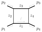
Figure 3: The one-loop box integral family contributing to Bhabha scattering.

The denominators are chosen as

$$z_{1}=\ell^{2}-m^{2},\quad z_{2}=(\ell-p_{1})^{2},\quad z_{3}=(\ell-p_{1}-p_{2})^{2}-m^{2},\quad z_{4}=(\ell-p_{1}-p_{2}-p_{3})^{2},$$ (68)

while the kinematics is specified by

$$p_{i}^{2}\ =\ m^{2}\ ,\qquad s\ =\ (p_{1}+p_{2})^{2}\ ,\qquad t\ =\ (p_{2}+p_{3})^{2}\ ,\qquad s+t+u\ =\ 4m^{2}\>.$$ (69)

There are $16$ possible sectors, and $7$ MIs depicted in Figure 4

Figure 4: The $7$ master integrals for the one-loop box integral family contributing to Bhabha scattering, before imposing symmetry relations.

For illustration purposes we consider here the Cut 24, associated to $z_{2}=z_{4}=0$. On this cut just four MIs contribute and we focus for concreteness on the decomposition of the target integral:

$$I\ =\ \int\ \mathrm{d}z_{1}\mathrm{d}z_{3}\ u(z_{1},z_{3})\frac{1}{z_{1}z_{3}^{2}}$$ (70)

in terms of master integrals

$$I\ =\ \sum_{i=1}^{4}c_{i}\ J_{i}\>,$$ (71)

depicted as

$$\vbox{\hbox{\parbox[c]{31.0761pt}{\includegraphics[scale={.6}]{figures/boxdotcut}}}}=c_{1}\vbox{\hbox{\includegraphics[scale={.6}]{figures/bubble1cut}}}+c_{2}\vbox{\hbox{\includegraphics[scale={.6}]{figures/tri1cut}}}+c_{3}\vbox{\hbox{\includegraphics[scale={.6}]{figures/tri2cut}}}+c_{4}\vbox{\hbox{\includegraphics[scale={.6}]{figures/boxcut}}}\>.$$ (72)

The twist is given by

$$u=B^{\gamma}\ ,\qquad\text{where}\qquad\gamma=\frac{d-5}{2}\>,$$ (73)

with:

$$B=-4m^{2}\left(st+(z_{1}-z_{3})^{2}\right)+s^{2}t-2s(t(z_{1}+z_{3})+2z_{1}z_{3})+t(z_{1}-z_{3})^{2}.$$ (74)

We may compute the connection as $\omega=\widehat{\omega}_{1}\>\mathrm{d}z_{1}+\widehat{\omega}_{3}\>\mathrm{d}z_{3}$ with

$$\widehat{\omega}_{1} = \frac{(d-5)\left(s(t+2z_{3})+(4m^{2}-t)(z_{1}-z_{3})\right)}{4m^{2}\left(st+(z_{1}-z_{3})^{2}\right)-s^{2}t+2st(z_{1}+z_{3})+4sz_{1}z_{3}-t(z_{1}-z_{3})^{2}}\>,$$ (75)

$$\widehat{\omega}_{3} = \frac{(d-5)\left(s(t+2z_{1})-(4m^{2}-t)(z_{1}-z_{3})\right)}{4m^{2}\left(st+(z_{1}-z_{3})^{2}\right)-s^{2}t+2st(z_{1}+z_{3})+4sz_{1}z_{3}-t(z_{1}-z_{3})^{2}}\>.$$ (76)

Choosing the variable order $\{z_{1},z_{3}\}$ and then following the procedure of Appendix B, we get as the dimension of the inner and outer bases

$$\nu^{(3)}\ =\ 2\>,\qquad\nu^{(13)}\ =\ 4\>.$$ (77)

The bases are

$$\begin{split}e^{(3)}=\left\{1\,,\;\frac{1}{z_{3}}\right\},\qquad e=e^{(13)}=\left\{1\,,\;\frac{1}{z_{1}}\,,\;\frac{1}{z_{3}}\,,\;\frac{1}{z_{1}z_{3}}\right\}\>,\end{split}$$ (78)

while the dual bases are chosen as

$$\begin{split}h^{(3)}=\{1,\delta_{3}\},\qquad h=h^{(13)}=\{1,\delta_{1},\delta_{3},\delta_{13}\}\>.\end{split}$$ (79)

The target left form associated to the integral on the LHS of eq. (72) is $\varphi_{L}=\tfrac{1}{z_{1}z_{3}^{2}}\>$.

Computation

Inner layer $z_{3}$:

We first have to compute the ${\bf C}$-matrix for the inner layer.

In order to do so we first find the $\mathcal{B}\ =\ B^{(3)}-\beta$ function for the internal layer, which is needed to compute the sum over finite poles using the polynomial residue algorithm explained in Section 3. $B^{(3)}$ is the denominator of $\Omega^{\vee(3)}=-\omega_{3}\>$, which in this case corresponds to the Baikov polynomial, given by:

$$B^{(3)}\ =\ 4m^{2}\left(st+(z_{1}-z_{3})^{2}\right)-s^{2}t+2st(z_{1}+z_{3})+4sz_{1}z_{3}-t(z_{1}-z_{3})^{2}\>.$$ (80)

We notice that $z_{3}=0$ is not a zero of $B^{(3)}$, since it is an unregulated pole. The intersection numbers between cocycles which do not contain any delta-forms are evaluated as in eq. (16)

$$\langle e_{i}^{(3)}|h_{1}^{(3)}\rangle = -\text{Res}_{\langle B^{(3)}\rangle}(e_{i}^{(3)}\psi_{R}^{(3)})\ -\ \text{Res}_{z=\infty}(e_{i}^{(3)}\psi_{R}^{(3)})\>,$$ (81)

while intersections with delta-forms read

$$\langle e_{i}^{(3)}|h_{2}^{(3)}\rangle = \langle e_{i}^{(3)}|\delta_{3}\rangle\ =\ \text{Res}_{z_{3}=0}(e_{i}^{(3)})\>.$$ (82)

Performing the computations one gets the internal ${\bf C}$-matrix, which is then given by:

$${\bf C}^{(3)} = \left(\begin{array}[]{cc}\frac{-4(d-5)s\left(4m^{2}-s-t\right)\left(m^{2}t+z(t+z)\right)}{(d-6)(d-4)\left(4m^{2}-t\right)^{2}}&0\\ \frac{z\left(4m^{2}-2s-t\right)-st}{(d-6)\left(4m^{2}-t\right)}&1\end{array}\right)\>.$$ (85)

Outer layer $z_{1}$:

The $\Omega^{\vee(1)}$ matrix for the outer layer is given as in eq. (24):

$$\Omega^{\vee(1)}\ =\ \left(\begin{array}[]{cc}\frac{(d-6)(t+2z_{1})}{2\left(m^{2}t+z_{1}(t+z_{1})\right)}&0\\ \frac{t\left(2m^{2}-s+z_{1}\right)}{2\left(m^{2}t+z_{1}(t+z_{1})\right)}&\;\frac{(d-5)\left(4m^{2}z_{1}+st-tz_{1}\right)}{4m^{2}\left(st+z_{1}^{2}\right)-t(s-z_{1})^{2}}\\ \end{array}\right)\>.$$ (88)

In order to use the polynomial division algorithm in the outer layer, one has to find the corresponding ideal generator $\mathcal{B}^{(1)}_{\beta}\ =\ B^{(1)}-\beta$ needed to compute the sum over finite poles. According to eq. (42), it is given in terms of

$$B^{(1)} = \mathrm{LCM}(\mathcal{P}^{(1)}_{\mathrm{fin}})\ =\ 2\left(m^{2}t+z_{1}(t+z_{1})\right)\left(4m^{2}\left(st+z_{1}^{2}\right)-t(s-z_{1})^{2}\right)\>.$$ (89)

The ${\bf C}$-matrix for the outer layer reads:

$${\bf C}^{(1)}\ =\ \left(\begin{array}[]{cccc}\frac{st^{2}\left(4m^{2}-s-t\right)}{4(d-7)(d-3)}&0&0&0\\ \frac{st^{2}\left((8d-44)m^{2}-(d-6)t\right)\left(4m^{2}-s-t\right)}{2(d-7)(d-6)(d-4)\left(4m^{2}-t\right)^{2}}&-\frac{4(d-5)m^{2}st\left(4m^{2}-s-t\right)}{(d-6)(d-4)\left(4m^{2}-t\right)^{2}}&0&0\\ \frac{st^{2}\left((8d-44)m^{2}-(d-6)t\right)\left(4m^{2}-s-t\right)}{2(d-7)(d-6)(d-4)\left(4m^{2}-t\right)^{2}}&0&-\frac{4(d-5)m^{2}st\left(4m^{2}-s-t\right)}{(d-6)(d-4)\left(4m^{2}-t\right)^{2}}&0\\ \frac{st^{2}}{(d-7)(d-6)\left(4m^{2}-t\right)}&\frac{-st}{(d-6)\left(4m^{2}-t\right)}&\frac{-st}{(d-6)\left(4m^{2}-t\right)}&1\\ \end{array}\right)\>.$$ (90)

When computing the intersection numbers of ${\varphi}$ in the outer basis, we remove the higher order pole as:

$${\varphi} = \frac{1}{z_{1}z_{3}^{2}}\ \sim\ \frac{\partial_{z_{3}}(u)}{u}\frac{1}{z_{1}z_{3}}\ =\ \frac{\omega_{3}}{z_{1}z_{3}}\ ,$$ (91)

where the $\sim$ means that the forms belong to the same cohomology class. Then we get:

$$\langle{\varphi}|h_{j}^{(13)}\rangle = \left(\begin{array}[]{cccc}\frac{(d-5)st}{(d-7)(d-6)\left(4m^{2}-t\right)}\ ,&\frac{d-5}{6-d}\ ,&\ \ \frac{(d-5)\left(4m^{2}-2s-t\right)}{(d-6)\left(4m^{2}-t\right)}\ ,&\ \ \frac{d-5}{4m^{2}-s}\\ \end{array}\right)\>.$$ (93)

Combining this result with the metric ${\bf C}^{(1)}$ via the master decomposition formula eq. (8) we get the coefficients of the reduction:

$$\langle{\varphi}|\mathcal{C}] = c_{1}\langle e_{1}|\mathcal{C}]\ +\ c_{2}\langle e_{2}|\mathcal{C}]\ +\ c_{3}\langle e_{3}|\mathcal{C}]\ +\ c_{4}\langle e_{4}|\mathcal{C}]\ ,$$ (94)

which are given by:

$$c_{1}\ =\ -\frac{d-3}{m^{2}t\left(4m^{2}-s\right)}\ ,\qquad\qquad\ c_{2}\ =\ \frac{(d-4)\left(4m^{2}-t\right)}{st\left(4m^{2}-s\right)}\ ,$$

$$c_{3}\ =\ -\frac{(d-4)\left(2m^{2}-s\right)\left(4m^{2}-t\right)}{2m^{2}st\left(4m^{2}-s\right)}\ ,\qquad\ c_{4}\ =\ \frac{d-5}{4m^{2}-s}\ ,$$ (95)

and are in agreement with FIRE.

More generally, the full decomposition can be achieved by combining the decompositions on different cuts, and in the following we will see it in some two-loop examples.

5.2 Planar double-box

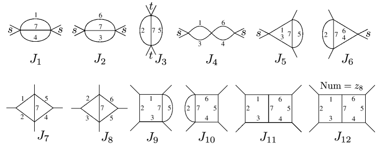
Figure 5: The 12 master integrals for the planar double box integral family, before imposing symmetry relations. The index $i$, next to the propagators, indicates the corresponding $z_{i}$ variable; $\mathrm{Num}$ stands for the numerator factor; $s,t,$ and $u$ channels are indicated, to distinguish among graphs with identical shape, but corresponding to different integrals.

The integral family of the planar double-box is given in terms of

$$z_{1} =k_{1}^{2}\>, z_{2} =(k_{1}{-}p_{1})^{2}, z_{3} =(k_{1}{-}p_{1}{-}p_{2})^{2}, z_{4} =(k_{2}{-}p_{1}{-}p_{2})^{2}, z_{5} =(k_{2}{+}p_{4})^{2},$$

$$z_{6} =k_{2}^{2}\>, z_{7} =(k_{1}{-}k_{2})^{2}, z_{8} =(k_{1}{+}p_{4})^{2}, z_{9} =(k_{2}{-}p_{1})^{2},$$ (96)

where $z_{8}$ and $z_{9}$ are irreducible scalar products, hence they may only appear in the numerator. The kinematics is such that:

$$p_{i}^{2}\ =\ 0\;,\qquad s\ =\ (p_{1}{+}p_{2})^{2}\;,\qquad t\ =\ (p_{1}{+}p_{4})^{2}\;,\qquad s+t+u\ =\ 0\;.$$ (97)

This integral family has (before application of the symmetry relations) 12 master integrals, which we may pick as depicted in Figure 5. We are interested in decomposing the target integral:

$$I\ =\ \int\ \mathrm{d}\mathbf{z}\ u(\mathbf{z})\frac{z_{8}^{2}}{z_{1}z_{2}z_{3}z_{4}z_{5}z_{6}z_{7}}$$ (98)

in terms of master integrals via a complete set of spanning cuts, as:

$$I\ =\ \sum_{i=1}^{12}c_{i}\ J_{i}\>.$$ (99)

The explicit expressions for the twist $u(\mathbf{z})$ as well as the master integrals $J_{i}$ can be found in the ancillary file Dbox_massless.m.

The set of spanning cuts is given by the maximal cuts of the first six master integrals $\{J_{1},\ldots,J_{6}\}$, and we will now go through them one by one.

Cut 147, maximal cut of $J_{1}$

Setting $z_{1}\ =\ z_{4}\ =\ z_{7}\ =\ 0$, and choosing as order of variables, from outer to inner:

$$\{z_{3},\ z_{8},\ z_{2},\ z_{6},\ z_{5},\ z_{9}\}$$ (100)

we get as dimensions for the various layers:

$$\nu^{(9)}\ =\ 1\>,\quad\nu^{(59)}\ =\ 2\>,\quad\nu^{(659)}\ =\ 2\>,\quad\nu^{(2659)}\ =\ 4\>,\quad\nu^{(82659)}\ =\ 5\>,\quad\nu^{(382659)}\ =\ 4\>.$$ (101)

We pick as bases:

$$\qquad\qquad\begin{aligned} e^{(9)}&=\left\{1\right\}\>,&e^{(59)}&=\left\{1,\tfrac{1}{z_{5}}\right\}\>,&e^{(659)}&=\left\{1,\tfrac{1}{z_{5}z_{6}}\right\}\>,\end{aligned}$$

$$\begin{aligned} e^{(2659)}&=\left\{1,\tfrac{1}{z_{2}},\tfrac{1}{z_{5}z_{6}},\tfrac{1}{z_{2}z_{5}z_{6}}\right\}\>,&e^{(82659)}&=\left\{1,\tfrac{1}{z_{5}},\tfrac{1}{z_{2}z_{5}},\tfrac{1}{z_{2}z_{5}z_{6}},\tfrac{z_{8}}{z_{2}z_{5}z_{6}},\right\}\>.\end{aligned}$$

$$\qquad\qquad\qquad\begin{aligned} e&=e^{(382659)}=\left\{1,\tfrac{1}{z_{2}z_{5}},\tfrac{1}{z_{2}z_{3}z_{5}z_{6}},\tfrac{z_{8}}{z_{2}z_{3}z_{5}z_{6}}\right\}\>.\end{aligned}$$ (102)

and as corresponding dual ones:

$$\qquad\qquad\begin{aligned} h^{(9)}&=\left\{1\right\}\>,&h^{(59)}&=\left\{1,\delta_{5}\right\}\>,&h^{(659)}&=\left\{1,\delta_{56}\right\}\>,\end{aligned}$$

$$\begin{aligned} h^{(2659)}&=\left\{1,\delta_{2},\delta_{56},\delta_{256}\right\}\>,&h^{(82659)}&=\left\{1,\delta_{5},\delta_{25},\delta_{256},z_{8}\delta_{256}\right\}\>,\end{aligned}$$

$$\qquad\qquad\,\,\begin{aligned} h&=h^{(382659)}=\left\{1,\delta_{25},\delta_{2356},z_{8}\delta_{2356}\right\}\>.\end{aligned}$$ (103)

We can then decompose the target left form: $\varphi\ =\ \frac{z_{8}^{2}}{z_{2}z_{3}z_{5}z_{6}}$ in terms of the outer basis, where we omit the superscripts for simplicity, obtaining:

$$\langle\varphi|\mathcal{C}]\ =\ c_{1}\langle e_{1}|\mathcal{C}]\ +\ c_{7}\langle e_{2}|\mathcal{C}]\ +\ c_{11}\langle e_{3}|\mathcal{C}]\ +\ c_{12}\langle e_{4}|\mathcal{C}]\>.$$ (104)

Cut 367, maximal cut of $J_{2}$

Setting $z_{3}\ =\ z_{6}\ =\ z_{7}\ =\ 0$, and choosing as order of variables, from outer to inner:

$$\{z_{1},\ z_{8},\ z_{2},\ z_{5},\ z_{4},\ z_{9}\}$$ (105)

we get as dimensions for the various layers:

$$\nu^{(9)}\ =\ 1\>,\quad\nu^{(49)}\ =\ 2\>,\quad\nu^{(549)}\ =\ 2\>,\quad\nu^{(2549)}\ =\ 4\>,\quad\nu^{(82549)}\ =\ 5\>,\quad\nu^{(182549)}\ =\ 4\>.$$ (106)

We pick as bases:

$$\qquad\qquad\qquad\begin{aligned} e^{(9)}&=\left\{1\right\}\>,&e^{(49)}&=\left\{1,\tfrac{1}{z_{4}}\right\}\>,&e^{(549)}&=\left\{1,\tfrac{1}{z_{4}z_{5}}\right\}\>,\end{aligned}$$

$$\begin{aligned} e^{(2549)}&=\left\{1,\tfrac{1}{z_{2}},\tfrac{1}{z_{4}z_{5}},\tfrac{1}{z_{2}z_{4}z_{5}}\right\}\>,&e^{(82549)}&=\left\{1,\tfrac{1}{z_{5}},\tfrac{1}{z_{2}z_{5}},\tfrac{1}{z_{2}z_{4}z_{5}},\tfrac{z_{8}}{z_{2}z_{4}z_{5}}\right\}\>,\end{aligned}$$

$$\qquad\qquad\qquad\,\,\begin{aligned} e&=e^{(182549)}=\left\{1,\tfrac{1}{z_{2}z_{5}},\tfrac{1}{z_{1}z_{2}z_{4}z_{5}},\tfrac{z_{8}}{z_{1}z_{2}z_{4}z_{5}}\right\}\>.\end{aligned}$$ (107)

and as corresponding dual ones:

$$\qquad\qquad\begin{aligned} h^{(9)}&=\left\{1\right\}\>,&h^{(49)}&=\left\{1,\delta_{4}\right\}\>,&h^{(549)}&=\left\{1,\delta_{45}\right\}\>,\end{aligned}$$

$$\begin{aligned} h^{(2549)}&=\left\{1,\delta_{2},\delta_{45},\delta_{245}\right\}\>,&h^{(82549)}&=\left\{1,\delta_{5},\delta_{25},\delta_{245},z_{8}\delta_{245}\right\}\>,\end{aligned}$$

$$\qquad\qquad\,\,\begin{aligned} h&=h^{(182549)}=\left\{1,\delta_{25},\delta_{1245},z_{8}\delta_{1245}\right\}\>.\end{aligned}$$ (108)

We can then decompose the target left form: $\varphi\ =\ \frac{z_{8}^{2}}{z_{1}z_{2}z_{4}z_{5}}$ in terms of the outer basis, where we omit the superscripts for simplicity, obtaining:

$$\langle\varphi|\mathcal{C}]\ =\ c_{2}\langle e_{1}|\mathcal{C}]\ +\ c_{8}\langle e_{2}|\mathcal{C}]\ +\ c_{11}\langle e_{3}|\mathcal{C}]\ +\ c_{12}\langle e_{4}|\mathcal{C}]\>.$$ (109)

Cut 257, maximal cut of $J_{3}$

Setting $z_{2}\ =\ z_{5}\ =\ z_{7}\ =\ 0$, and choosing as order of variables, from outer to inner:

$$\{z_{1},\ z_{8},\ z_{3},\ z_{6},\ z_{4},\ z_{9}\}$$ (110)

we get as dimensions for the various layers:

$$\nu^{(9)}\ =\ 1\>,\quad\nu^{(49)}\ =\ 2\>,\quad\nu^{(649)}\ =\ 2\>,\quad\nu^{(3649)}\ =\ 6\>,\quad\nu^{(83649)}\ =\ 10\>,\quad\nu^{(183649)}\ =\ 7\>.$$ (111)

We pick as bases:

$$\qquad\qquad\begin{aligned} e^{(9)}&=\left\{1\right\}\>,&e^{(49)}&=\left\{1,\tfrac{1}{z_{4}}\right\}\>,&e^{(649)}&=\left\{1,\tfrac{1}{z_{4}z_{6}}\right\}\>,\end{aligned}$$

$$\qquad\qquad\qquad\,\,\,\,\,\begin{aligned} e^{(3649)}&=\left\{1,\tfrac{1}{z_{3}},\tfrac{1}{z_{4}},\tfrac{1}{z_{4}z_{6}},\tfrac{z_{9}}{z_{4}z_{6}},\tfrac{1}{z_{3}z_{4}z_{6}}\right\}\>,\end{aligned}$$

$$\qquad\,\,\begin{aligned} e^{(83649)}&=\left\{1,\tfrac{1}{z_{3}},\tfrac{1}{z_{4}},\tfrac{z_{8}}{z_{4}},\tfrac{1}{z_{6}},\tfrac{1}{z_{3}z_{6}},\tfrac{1}{z_{4}z_{6}},\tfrac{z_{8}}{z_{4}z_{6}},\tfrac{1}{z_{3}z_{4}z_{6}},\tfrac{z_{8}}{z_{3}z_{4}z_{6}}\right\}\>,\end{aligned}$$

$$\qquad\,\,\begin{aligned} e&=e^{(183649)}=\left\{1,\tfrac{1}{z_{1}z_{4}},\tfrac{1}{z_{3}z_{6}},\tfrac{1}{z_{1}z_{3}},\tfrac{1}{z_{4}z_{6}},\tfrac{1}{z_{1}z_{3}z_{4}z_{6}},\tfrac{z_{8}}{z_{1}z_{3}z_{4}z_{6}}\right\}\>.\end{aligned}$$ (112)

and as corresponding dual ones:

$$\qquad\qquad\begin{aligned} h^{(9)}&=\left\{1\right\}\>,&h^{(49)}&=\left\{1,\delta_{4}\right\}\>,&h^{(649)}&=\left\{1,\delta_{46}\right\}\>,\end{aligned}$$

$$\qquad\qquad\qquad\begin{aligned} h^{(3649)}&=\left\{1,\delta_{3},\delta_{4},\delta_{46},z_{9}\delta_{46},\delta_{346}\right\}\>,\end{aligned}$$

$$\qquad\,\,\,\begin{aligned} h^{(83649)}&=\left\{1,\delta_{3},\delta_{4},z_{8}\delta_{4},\delta_{6},\delta_{36},\delta_{46},z_{8}\delta_{46},\delta_{346},z_{8}\delta_{346}\right\}\>,\end{aligned}$$

$$\qquad\,\,\,\begin{aligned} h&=h^{(183649)}=\left\{1,\delta_{14},\delta_{36},\delta_{13},\delta_{46},\delta_{1346},z_{8}\delta_{1346}\right\}\>.\end{aligned}$$ (113)

We can then decompose the target left form: $\varphi\ =\ \frac{z_{8}^{2}}{z_{1}z_{3}z_{4}z_{6}}$ in terms of the outer basis, where we omit the superscripts for simplicity, obtaining:

$$\langle\varphi|\mathcal{C}]\ =\ c_{3}\langle e_{1}|\mathcal{C}]\ +\ c_{7}\langle e_{2}|\mathcal{C}]\ +\ c_{8}\langle e_{3}|\mathcal{C}]\ +\ c_{9}\langle e_{4}|\mathcal{C}]\ +\ c_{10}\langle e_{5}|\mathcal{C}]\ +\ c_{11}\langle e_{6}|\mathcal{C}]\ +\ c_{12}\langle e_{7}|\mathcal{C}]\>.$$ (114)

Cut 1346, maximal cut of $J_{4}$

Setting $z_{1}\ =\ z_{3}\ =\ z_{4}\ =\ z_{6}\ =\ 0$, and choosing as order of variables, from outer to inner:

$$\{z_{8},\ z_{2},\ z_{5},\ z_{7},\ z_{9}\}$$ (115)

we get as dimensions for the various layers:

$$\nu^{(9)}\ =\ 1\>,\quad\nu^{(79)}\ =\ 2\>,\quad\nu^{(579)}\ =\ 2\>,\quad\nu^{(2579)}\ =\ 4\>,\quad\nu^{(82579)}\ =\ 3\>.$$ (116)

We pick as bases:

$$\qquad\qquad\begin{aligned} e^{(9)}&=\left\{1\right\}\>,&e^{(79)}&=\left\{1,\tfrac{1}{z_{7}}\right\}\>,&e^{(579)}&=\left\{1,\tfrac{1}{z_{5}z_{7}}\right\}\>,&\end{aligned}$$

$$\qquad\begin{aligned} \qquad\qquad\qquad&e^{(2579)}=\left\{1,\tfrac{1}{z_{2}},\tfrac{1}{z_{5}z_{7}},\tfrac{1}{z_{2}z_{5}z_{7}}\right\},\ \\ e=&e^{(82579)}=\left\{1,\tfrac{1}{z_{2}z_{5}z_{7}},\tfrac{z_{8}}{z_{2}z_{5}z_{7}}\right\},\end{aligned}$$ (117)

and as corresponding dual ones:

$$\qquad\begin{aligned} h^{(9)}&=\left\{1\right\}\>,&h^{(79)}&=\left\{1,\delta_{7}\right\}\>,&h^{(579)}&=\left\{1,\delta_{57}\right\}\>,\end{aligned}$$

$$\qquad\begin{aligned} \qquad\qquad\qquad&h^{(2579)}=\left\{1,\delta_{2},\delta_{57},\delta_{257}\right\},\ \\ h=&h^{(82579)}=\left\{1,\delta_{257},z_{8}\delta_{257}\right\}.\end{aligned}$$ (118)

We can then decompose the target left form: $\varphi\ =\ \frac{z_{8}^{2}}{z_{2}z_{5}z_{7}}$ in terms of the outer basis, where we omit the superscripts for simplicity, obtaining:

$$\langle\varphi|\mathcal{C}]\ =\ c_{4}\langle e_{1}|\mathcal{C}]\ +\ c_{11}\langle e_{2}|\mathcal{C}]\ +\ c_{12}\langle e_{3}|\mathcal{C}]\>.$$ (119)

Cut 1357, maximal cut of $J_{5}$

Setting $z_{1}\ =\ z_{3}\ =\ z_{5}\ =\ z_{7}\ =\ 0$, and choosing as order of variables, from outer to inner:

$$\{z_{8},\ z_{2},\ z_{4},\ z_{6},\ z_{9}\}$$ (120)

we get as dimensions for the various layers:

$$\nu^{(9)}\ =\ 1\>,\quad\nu^{(69)}\ =\ 2\>,\quad\nu^{(469)}\ =\ 2\>,\quad\nu^{(2469)}\ =\ 4\>,\quad\nu^{(82469)}\ =\ 4\>.$$ (121)

We pick as bases:

$$\qquad\qquad\begin{aligned} e^{(9)}&=\left\{1\right\}\>,&e^{(69)}&=\left\{1,\tfrac{1}{z_{6}}\right\}\>,&e^{(469)}&=\left\{1,\tfrac{1}{z_{4}z_{6}}\right\}\>,&\end{aligned}$$

$$\qquad\begin{aligned} \qquad\qquad\qquad&e^{(2469)}=\left\{1,\tfrac{1}{z_{2}},\tfrac{1}{z_{4}z_{6}},\tfrac{1}{z_{2}z_{4}z_{6}}\right\},\ \\ e=&e^{(82469)}=\left\{1,\tfrac{1}{z_{2}},\tfrac{1}{z_{2}z_{4}z_{6}},\tfrac{z_{8}}{z_{2}z_{5}z_{6}}\right\},\end{aligned}$$ (122)

and as corresponding dual ones:

$$\qquad\begin{aligned} h^{(9)}&=\left\{1\right\}\>,&h^{(69)}&=\left\{1,\delta_{6}\right\}\>,&h^{(469)}&=\left\{1,\delta_{46}\right\}\>,\end{aligned}$$

$$\qquad\begin{aligned} \qquad\qquad\qquad&h^{(2469)}=\left\{1,\delta_{2},\delta_{46},\delta_{246}\right\},\ \\ h=&h^{(82469)}=\left\{1,\delta_{2},\delta_{246},z_{8}\delta_{246}\right\}.\end{aligned}$$ (123)

We can then decompose the target left form: $\varphi\ =\ \frac{z_{8}^{2}}{z_{2}z_{4}z_{6}}$ in terms of the outer basis, where we omit the superscripts for simplicity, obtaining:

$$\langle\varphi|\mathcal{C}]\ =\ c_{5}\langle e_{1}|\mathcal{C}]\ +\ c_{9}\langle e_{2}|\mathcal{C}]\ +\ c_{11}\langle e_{3}|\mathcal{C}]\ +\ c_{12}\langle e_{4}|\mathcal{C}]\>.$$ (124)

Cut 2467, maximal cut of $J_{6}$

Setting $z_{2}\ =\ z_{4}\ =\ z_{6}\ =\ z_{7}\ =\ 0$, and choosing as order of variables, from outer to inner:

$$\{z_{9},\ z_{1},\ z_{3},\ z_{5},\ z_{8}\}$$ (125)

we get as dimensions for the various layers:

$$\nu^{(8)}\ =\ 1\>,\quad\nu^{(58)}\ =\ 2\>,\quad\nu^{(358)}\ =\ 4\>,\quad\nu^{(1358)}\ =\ 4\>,\quad\nu^{(91358)}\ =\ 4\>.$$ (126)

We pick as bases bases:

$$\qquad\qquad\begin{aligned} e^{(8)}&=\left\{1\right\}\>,&e^{(58)}&=\left\{1,\tfrac{1}{z_{5}}\right\}\>,&e^{(358)}&=\left\{1,\tfrac{1}{z_{3}},\tfrac{1}{z_{5}},\tfrac{1}{z_{3}z_{5}}\right\}\>,&\end{aligned}$$

$$\qquad\qquad\quad\begin{aligned} \qquad\qquad\qquad&e^{(1358)}=\left\{1,\tfrac{1}{z_{5}},\tfrac{1}{z_{1}z_{3}},\tfrac{1}{z_{1}z_{3}z_{5}}\right\},\ \\ e=&e^{(91358)}=\left\{1,\tfrac{1}{z_{5}},\tfrac{1}{z_{1}z_{3}z_{5}},\tfrac{z_{8}}{z_{1}z_{3}z_{5}}\right\},\end{aligned}$$ (127)

and as corresponding dual ones:

$$\qquad\begin{aligned} h^{(8)}&=\left\{1\right\}\>,&h^{(58)}&=\left\{1,\delta_{5}\right\}\>,&h^{(358)}&=\left\{1,\delta_{3},\delta_{5},\delta_{35}\right\}\>,\end{aligned}$$

$$\qquad\qquad\begin{aligned} \qquad\qquad\qquad&h^{(1358)}=\left\{1,\delta_{5},\delta_{13},\delta_{135}\right\},\ \\ h=&h^{(91358)}=\left\{1,\delta_{5},\delta_{135},z_{8}\delta_{135}\right\}.\end{aligned}$$ (128)

We can then decompose the target left form: $\varphi\ =\ \frac{z_{8}^{2}}{z_{1}z_{3}z_{5}}$ in terms of the outer basis, where we omit the superscripts for simplicity, obtaining:

$$\langle\varphi|\mathcal{C}]\ =\ c_{6}\langle e_{1}|\mathcal{C}]\ +\ c_{10}\langle e_{2}|\mathcal{C}]\ +\ c_{11}\langle e_{3}|\mathcal{C}]\ +\ c_{12}\langle e_{4}|\mathcal{C}]\>.$$ (129)

Cut merging and symmetries

From the analysis on the complete spanning cuts, one is able to get the coefficients of the decomposition, obtaining:

$$c_{1}=c_{2}=\frac{(3d-10)(3d-8)(s+2t)}{(d-4)^{2}(d-3)s^{3}}\>,\>c_{3}=\frac{9(3d-10)(3d-8)}{(d-4)^{2}st}\>,\>$$

$$c_{4}=\frac{2(2ds+2dt-7s-8t)}{(d-4)s^{2}}\>,\>c_{5}=\frac{9(3d-10)}{2(d-4)s}\>,\>c_{6}=\frac{(3d-10)(2s-t)}{(d-4)s^{2}}\>,\>$$ (130)

$$c_{7}=c_{8}=-\frac{(d-4)(7s+9t)}{2(d-3)s}\>,\>c_{9}=c_{10}=4\>,\>c_{11}=\frac{(d-4)st}{2(d-3)}\>,\>c_{12}=-\frac{3ds-12s-2t}{2(d-3)}\>.$$

Symmetries of the problem induce the following additional symmetry relations between the master integrals:

$$J_{1}\ =\ J_{2}\>,\qquad J_{5}\ =\ J_{6}\>,\qquad J_{7}\ =\ J_{8}\>,\qquad J_{9}\ =\ J_{10}\>.$$ (131)

This reduce to 8 the number of genuinely independent master integrals, meaning that the final decomposition may be written as

$$I=\tilde{c}_{1}J_{1}+c_{3}J_{3}+c_{4}J_{4}+\tilde{c}_{5}J_{5}+\tilde{c}_{7}J_{7}+\tilde{c}_{9}J_{9}+c_{11}J_{11}+c_{12}J_{12}\>,$$ (132)

where

$$\tilde{c}_{1}=c_{1}+c_{2}\>,\qquad\tilde{c}_{5}=c_{5}+c_{6}\>,\qquad\tilde{c}_{7}=c_{7}+c_{8}\>,\qquad\tilde{c}_{9}=c_{9}+c_{10}\>.$$ (133)

5.3 Non-planar double-box

Figure 6: The 16 master integrals for the non-planar double-box integral family, before imposing symmetry relations. The index $i$, next to the propagators, indicates the corresponding $z_{i}$ variable; $\mathrm{Num}$ stands for the numerator factor; $s,t,$ and $u$ channels are indicated, to distinguish among graphs with identical shape, but corresponding to different integrals.

The integral family of the non-planar double box is given in terms of

$$z_{1} =k_{1}^{2}\>, z_{2} =(k_{1}{-}p_{1})^{2}, z_{3} =(k_{1}{-}p_{1}{-}p_{2})^{2}, z_{4} =(k_{2}{-}p_{1}{-}p_{2}{-}p_{3})^{2}, z_{5} =k_{2}^{2}\>,$$

$$z_{6} =(k_{1}{-}k_{2})^{2}, z_{7} =(k_{1}{-}k_{2}{+}p_{3})^{2}, z_{8} =(k_{1}{-}p_{1}{-}p_{2}{-}p_{3})^{2}, z_{9} =(k_{2}{-}p_{1})^{2},$$ (134)

where $z_{8}$ and $z_{9}$ are irreducible scalar products. The kinematics is such that:

$$p_{i}^{2}\ =\ 0\>,\qquad s\ =\ (p_{1}{+}p_{2})^{2}\>,\qquad t\ =\ (p_{1}{+}p_{4})^{2}\>,\qquad s+t+u\ =\ 0\>.$$ (135)

This integral family has (before the application of symmetry relations) 16 master integrals, which we may pick as depicted in Figure 6. We are interested in decomposing the target integral:

$$I\ =\ \int\ \mathrm{d}\mathbf{z}\ u(\mathbf{z})\frac{z_{8}^{2}}{z_{1}z_{2}z_{3}z_{4}z_{5}z_{6}z_{7}}$$ (136)

in terms of master integrals via a complete set of spanning cuts, as:

$$I\ =\ \sum_{i=1}^{16}c_{i}\ J_{i}\>.$$ (137)

The explicit expressions for the twist $u(\mathbf{z})$ as well as the master integrals $J_{i}$ can be found in the ancillary file Dbox_massless_nonplanar.m.

The set of spanning cuts is given by the maximal cuts of the first six master integrals $\{J_{1},\ldots,J_{6}\}$, and we will now go through them one by one.

Cut 147, maximal cut of $J_{1}$

Setting $z_{1}\ =\ z_{4}\ =\ z_{7}\ =\ 0$, and choosing as order of variables, from outer to inner:

$$\{z_{8},\ z_{3},\ z_{2},\ z_{5},\ z_{6},\ z_{9}\}$$ (138)

we get as dimensions for the various layers:

$$\nu^{(9)}\ =\ 1\>,\quad\nu^{(69)}\ =\ 2\>,\quad\nu^{(569)}\ =\ 2\>,\quad\nu^{(2569)}\ =\ 4\>,\quad\nu^{(32569)}\ =\ 7\>,\quad\nu^{(832569)}\ =\ 6\>.$$ (139)

We pick as bases:

$$e^{(9)} = \left\{1\right\},\qquad\qquad\quad e^{(69)}=\left\{1,\tfrac{1}{z_{6}}\right\},\qquad\qquad\quad e^{(569)}=\left\{1,\tfrac{1}{z_{5}z_{6}}\right\},$$

$$e^{(2569)} = \left\{1,\tfrac{1}{z_{2}},\tfrac{1}{z_{5}z_{6}},\tfrac{1}{z_{2}z_{5}z_{6}}\right\},\qquad e^{(32569)}=\left\{1,\tfrac{1}{z_{2}},\tfrac{1}{z_{6}},\tfrac{1}{z_{2}z_{6}},\tfrac{1}{z_{2}z_{5}z_{6}},\tfrac{1}{z_{3}z_{5}z_{6}},\tfrac{1}{z_{2}z_{3}z_{5}z_{6}}\right\},$$

$$e = e^{(832569)}=\left\{1,\tfrac{1}{z_{2}z_{6}},\tfrac{1}{z_{2}z_{5}},\tfrac{1}{z_{3}z_{5}z_{6}},\tfrac{1}{z_{2}z_{3}z_{5}z_{6}},\tfrac{z_{8}}{z_{2}z_{3}z_{5}z_{6}}\right\},$$ (140)

and as corresponding dual ones:

$$h^{(9)}\ = \ \left\{1\right\},\qquad h^{(69)}\ =\ \left\{1,\delta_{6}\right\},\qquad h^{(569)}\ =\ \left\{1,\delta_{56}\right\},\$$

$$h^{(2569)} = \left\{1,\delta_{2},\delta_{56},\delta_{256}\right\},\qquad h^{(32569)}=\left\{1,\delta_{2},\delta_{6},\delta_{26},\delta_{256},\delta_{356},\delta_{2356}\right\},\$$

$$h = h^{(832569)}=\left\{1,\delta_{26},\delta_{25},\delta_{356},\delta_{2356},z_{8}\delta_{2356}\right\}\>.$$ (141)

We can then decompose the target left form: $\varphi\ =\ \frac{z_{8}^{2}}{z_{2}z_{3}z_{5}z_{6}}$ in terms of the outer basis, where we omit the superscripts for simplicity, obtaining:

$$\langle\varphi|\mathcal{C}]\ =\ c_{1}\langle e_{1}|\mathcal{C}]\ +\ c_{7}\langle e_{2}|\mathcal{C}]\ +\ c_{9}\langle e_{3}|\mathcal{C}]\ +\ c_{14}\langle e_{4}|\mathcal{C}]\ +\ c_{15}\langle e_{5}|\mathcal{C}]\ +\ c_{16}\langle e_{6}|\mathcal{C}]\>.$$ (142)

Cut 356, maximal cut of $J_{2}$

Setting $z_{3}\ =\ z_{5}\ =\ z_{6}\ =\ 0$, and choosing as order of variables, from outer to inner:

$$\{z_{8},\ z_{1},\ z_{2},\ z_{7},\ z_{4},\ z_{9}\}$$ (143)

we get as dimensions for the various layers:

$$\nu^{(9)}\ =\ 1\>,\quad\nu^{(49)}\ =\ 2\>,\quad\nu^{(749)}\ =\ 2\>,\quad\nu^{(2749)}\ =\ 4\>,\quad\nu^{(12749)}\ =\ 7\>,\quad\nu^{(812749)}\ =\ 6\>.$$ (144)

We pick as bases:

$$e^{(9)} = \left\{1\right\},\qquad e^{(49)}=\left\{1,\tfrac{1}{z_{4}}\right\},\qquad e^{(749)}=\left\{1,\tfrac{1}{z_{4}z_{7}}\right\},$$

$$e^{(2749)} = \left\{1,\tfrac{1}{z_{2}},\tfrac{1}{z_{4}z_{7}},\tfrac{1}{z_{2}z_{4}z_{7}}\right\},\qquad e^{(12749)}=\left\{1,\ \tfrac{1}{z_{2}},\tfrac{1}{z_{4}},\tfrac{1}{z_{2}z_{4}},\tfrac{1}{z_{2}z_{4}z_{7}},\tfrac{1}{z_{1}z_{4}z_{7}},\tfrac{1}{z_{1}z_{2}z_{4}z_{7}}\right\},$$

$$e = e^{(812749)}=\left\{1,\tfrac{1}{z_{2}z_{4}},\tfrac{1}{z_{2}z_{7}},\tfrac{1}{z_{1}z_{4}z_{7}},\tfrac{1}{z_{1}z_{2}z_{4}z_{7}},\tfrac{z_{8}}{z_{1}z_{2}z_{4}z_{7}}\right\},$$ (145)

and as corresponding dual ones:

$$h^{(9)}\ = \ \left\{1\right\},\qquad h^{(49)}\ =\ \left\{1,\delta_{4}\right\},\qquad h^{(749)}\ =\ \left\{1,\delta_{47}\right\},\$$

$$h^{(2749)} = \left\{1,\delta_{2},\delta_{47},\delta_{247}\right\},\qquad h^{(12749)}=\left\{1,\delta_{2},\delta_{4},\delta_{24},\delta_{247},\delta_{147},\delta_{1247}\right\},\$$

$$h = h^{(812749)}=\left\{1,\delta_{24},\delta_{27},\delta_{147},\delta_{1247},z_{8}\delta_{1247}\right\}\>.$$ (146)

We can then decompose the target left form: $\varphi\ =\ \frac{z_{8}^{2}}{z_{1}z_{2}z_{4}z_{7}}$ in terms of the outer basis, where we omit the superscripts for simplicity, obtaining:

$$\langle\varphi|\mathcal{C}]\ =\ c_{2}\langle e_{1}|\mathcal{C}]\ +\ c_{8}\langle e_{2}|\mathcal{C}]\ +\ c_{10}\langle e_{3}|\mathcal{C}]\ +\ c_{14}\langle e_{4}|\mathcal{C}]\ +\ c_{15}\langle e_{5}|\mathcal{C}]\ +\ c_{16}\langle e_{6}|\mathcal{C}]\>.$$ (147)

Cut 246, maximal cut of $J_{3}$

Setting $z_{2}\ =\ z_{4}\ =\ z_{6}\ =\ 0$, and choosing as order of variables, from outer to inner:

$$\{z_{3},\ z_{8},\ z_{1},\ z_{7},\ z_{5},\ z_{9}\}$$ (148)

we get as dimensions for the various layers:

$$\nu^{(9)}\ =\ 1\>,\quad\nu^{(59)}\ =\ 2\>,\quad\nu^{(759)}\ =\ 2\>,\quad\nu^{(1759)}\ =\ 6\>,\quad\nu^{(81759)}\ =\ 10\>,\quad\nu^{(381759)}\ =\ 7\>.$$ (149)

We pick as bases:

$$e^{(9)} = \left\{1\right\},\qquad e^{(59)}=\left\{1,\tfrac{1}{z_{5}}\right\},\qquad e^{(759)}=\left\{1,\tfrac{1}{z_{5}z_{7}}\right\},$$

$$e^{(1759)} = \left\{1,\tfrac{1}{z_{1}},\tfrac{1}{z_{5}},\tfrac{1}{z_{5}z_{7}},\tfrac{z_{9}}{z_{5}z_{7}},\tfrac{1}{z_{1}z_{5}z_{7}}\right\},$$

$$e^{(81759)} = \left\{1,\tfrac{1}{z_{1}},\tfrac{1}{z_{5}},\tfrac{z_{8}}{z_{5}},\tfrac{1}{z_{7}},\tfrac{1}{z_{1}z_{7}},\tfrac{1}{z_{5}z_{7}},\tfrac{z_{8}}{z_{5}z_{7}},\tfrac{1}{z_{1}z_{5}z_{7}},\tfrac{z_{8}}{z_{1}z_{5}z_{7}}\right\},$$

$$e = e^{(381759)}=\left\{1,\tfrac{1}{z_{1}z_{7}},\tfrac{1}{z_{3}z_{5}},\tfrac{1}{z_{5}z_{7}},\tfrac{1}{z_{1}z_{3}},\tfrac{1}{z_{1}z_{3}z_{5}z_{7}},\tfrac{z_{8}}{z_{1}z_{3}z_{5}z_{7}}\right\}\>,$$ (150)

and as corresponding dual ones:

$$h^{(9)}\ = \ \left\{1\right\},\qquad h^{(59)}\ =\ \left\{1,\delta_{5}\right\},\qquad h^{(759)}\ =\ \left\{1,\delta_{57}\right\},\$$

$$h^{(1759)} = \left\{1,\delta_{1},\delta_{5},\delta_{57},z_{9}\delta_{57},\delta_{157}\right\},$$

$$h^{(81759)} = \left\{1,\delta_{1},\delta_{5},z_{8}\delta_{5},\delta_{7},\delta_{17},\delta_{57},z_{8}\delta_{57},\delta_{157},z_{8}\delta_{157}\right\},$$

$$h = h^{(381759)}=\left\{1,\delta_{17},\delta_{35},\delta_{57},\delta_{13},\delta_{1357},z_{8}\delta_{1357}\right\}\>.$$ (151)

We can then decompose the target left form: $\varphi\ =\ \frac{z_{8}^{2}}{z_{1}z_{3}z_{5}z_{7}}$ in terms of the outer basis, where we omit the superscripts for simplicity, obtaining:

$$\langle\varphi|\mathcal{C}]\ =\ c_{3}\langle e_{1}|\mathcal{C}]\ +\ c_{7}\langle e_{2}|\mathcal{C}]\ +\ c_{8}\langle e_{3}|\mathcal{C}]\ +\ c_{11}\langle e_{4}|\mathcal{C}]\ +\ c_{12}\langle e_{5}|\mathcal{C}]\ +\ c_{15}\langle e_{6}|\mathcal{C}]\ +\ c_{16}\langle e_{7}|\mathcal{C}]\>.$$ (152)

Cut 257, maximal cut of $J_{4}$

Setting $z_{2}\ =\ z_{5}\ =\ z_{7}\ =\ 0$, and choosing as order of variables, from outer to inner:

$$\{z_{1},\ z_{8},\ z_{3},\ z_{6},\ z_{4},\ z_{9}\}$$ (153)

we get as dimensions for the various layers:

$$\nu^{(9)}\ =\ 1\>,\quad\nu^{(49)}\ =\ 2\>,\quad\nu^{(649)}\ =\ 2\>,\quad\nu^{(3649)}\ =\ 7\>,\quad\nu^{(83649)}\ =\ 10\>,\quad\nu^{(183649)}\ =\ 7\>.$$ (154)

We pick as bases:

$$e^{(9)} = \left\{1\right\},\qquad e^{(49)}=\left\{1,\tfrac{1}{z_{4}}\right\},\qquad e^{(649)}=\left\{1,\tfrac{1}{z_{4}z_{6}}\right\},$$

$$e^{(3649)} = \left\{1,z_{3},\tfrac{1}{z_{6}},\tfrac{1}{z_{3}},\tfrac{1}{z_{4}z_{6}},\tfrac{z_{3}}{z_{4}z_{6}},\tfrac{1}{z_{3}z_{4}z_{6}}\right\},$$

$$e^{(83649)} = \left\{1,\tfrac{1}{z_{3}},\tfrac{1}{z_{4}},\tfrac{z_{3}}{z_{4}},\tfrac{1}{z_{6}},\tfrac{1}{z_{3}z_{6}},\tfrac{1}{z_{4}z_{6}},\tfrac{z_{8}}{z_{4}z_{6}},\tfrac{1}{z_{3}z_{4}z_{6}},\tfrac{z_{8}}{z_{3}z_{4}z_{6}}\right\},$$

$$e = e^{(183649)}=\left\{1,\tfrac{1}{z_{1}z_{4}},\tfrac{1}{z_{3}z_{6}},\tfrac{1}{z_{4}z_{6}},\tfrac{1}{z_{1}z_{3}},\tfrac{1}{z_{1}z_{3}z_{4}z_{6}},\tfrac{z_{8}}{z_{1}z_{3}z_{4}z_{6}}\right\}\>,$$ (155)

and as corresponding dual ones:

$$h^{(9)}\ = \ \left\{1\right\},\qquad h^{(49)}\ =\ \left\{1,\delta_{4}\right\},\qquad h^{(649)}\ =\ \left\{1,\delta_{46}\right\},\$$

$$h^{(3649)} = \left\{1,z_{3},\delta_{6},\delta_{3},\delta_{46},z_{3}\delta_{46},\delta_{346}\right\},$$

$$h^{(83649)} = \left\{1,\delta_{3},\delta_{4},z_{3}\delta_{4},\delta_{6},\delta_{36},\delta_{46},z_{8}\delta_{46},\delta_{346},z_{8}\delta_{346}\right\},$$

$$h = h^{(183649)}=\left\{1,\delta_{14},\delta_{36},\delta_{46},\delta_{13},\delta_{1346},z_{8}\delta_{1346}\right\}\>.$$ (156)

We can then decompose the target left form: $\varphi\ =\ \frac{z_{8}^{2}}{z_{1}z_{3}z_{4}z_{6}}$ in terms of the outer basis, where we omit the superscripts for simplicity, obtaining:

$$\langle\varphi|\mathcal{C}]\ =\ c_{4}\langle e_{1}|\mathcal{C}]\ +\ c_{9}\langle e_{2}|\mathcal{C}]\ +\ c_{10}\langle e_{3}|\mathcal{C}]\ +\ c_{11}\langle e_{4}|\mathcal{C}]\ +\ c_{13}\langle e_{5}|\mathcal{C}]\ +\ c_{15}\langle e_{6}|\mathcal{C}]\ +\ c_{16}\langle e_{7}|\mathcal{C}]\>.$$ (157)

Cut 1346, maximal cut of $J_{5}$

Setting $z_{1}\ =\ z_{3}\ =\ z_{4}\ =\ z_{6}\ =\ 0$, and choosing as order of variables, from outer to inner:

$$\{z_{8},\ z_{2},\ z_{5},\ z_{7},\ z_{9}\}$$ (158)

we get as dimensions for the various layers:

$$\nu^{(9)}\ =\ 1\>,\quad\nu^{(79)}\ =\ 2\>,\quad\nu^{(579)}\ =\ 2\>,\quad\nu^{(2579)}\ =\ 4\>,\quad\nu^{(82579)}\ =\ 5\>.$$ (159)

We pick as bases:

$$e^{(9)} = \left\{1\right\},\qquad e^{(79)}=\left\{1,\tfrac{1}{z_{7}}\right\},\qquad e^{(579)}=\left\{1,\tfrac{1}{z_{5}z_{7}}\right\},$$ (160)

$$\quad\,e^{(2579)}=\left\{1,\tfrac{1}{z_{2}},\tfrac{1}{z_{5}z_{7}},\tfrac{1}{z_{2}z_{5}z_{7}}\right\},$$

$$e =e^{(82579)}=\left\{1,\tfrac{1}{z_{2}},\tfrac{1}{z_{5}z_{7}},\tfrac{1}{z_{2}z_{5}z_{7}},\tfrac{z_{8}}{z_{2}z_{5}z_{7}}\right\}\>,$$

and as corresponding dual ones:

$$h^{(9)}\ = \ \left\{1\right\},\ \ h^{(79)}\ =\ \left\{1,\delta_{7}\right\},\ \ h^{(579)}\ =\ \left\{1,\delta_{57}\right\},$$

$$h^{(2579)}=\left\{1,\delta_{2},\delta_{57},\delta_{257}\right\},$$

$$h = h^{(82579)}=\left\{1,\delta_{2},\delta_{57},\delta_{257},z_{8}\delta_{257}\right\}\>.$$ (161)

We can then decompose the target left form: $\varphi\ =\ \frac{z_{8}^{2}}{z_{2}z_{5}z_{7}}$ in terms of the outer basis, where we omit the superscripts for simplicity, obtaining:

$$\langle\varphi|\mathcal{C}]\ =\ c_{5}\langle e_{1}|\mathcal{C}]\ +\ c_{12}\langle e_{2}|\mathcal{C}]\ +\ c_{14}\langle e_{3}|\mathcal{C}]\ +\ c_{15}\langle e_{4}|\mathcal{C}]\ +\ c_{16}\langle e_{5}|\mathcal{C}]\>.$$ (162)

Cut 1357, maximal cut of $J_{6}$

Setting $z_{1}\ =\ z_{3}\ =\ z_{5}\ =\ z_{7}\ =\ 0$, and choosing as order of variables, from outer to inner:

$$\{z_{8},\ z_{2},\ z_{4},\ z_{6},\ z_{9}\}$$ (163)

we get as dimensions for the various layers:

$$\nu^{(9)}\ =\ 1\>,\quad\nu^{(69)}\ =\ 2\>,\quad\nu^{(469)}\ =\ 2\>,\quad\nu^{(2469)}\ =\ 4\>,\quad\nu^{(82469)}\ =\ 5\>.$$ (164)

We pick as bases:

$$e^{(9)} = \left\{1\right\},\ \ e^{(69)}=\left\{1,\tfrac{1}{z_{6}}\right\},\ \ e^{(469)}=\left\{1,\tfrac{1}{z_{4}z_{6}}\right\},$$ (165)

$$\quad\,e^{(2469)}=\left\{1,\tfrac{1}{z_{2}},\tfrac{1}{z_{4}z_{6}},\tfrac{1}{z_{2}z_{4}z_{6}}\right\},$$

$$e =e^{(82469)}=\left\{1,\tfrac{1}{z_{2}},\tfrac{1}{z_{4}z_{6}},\tfrac{1}{z_{2}z_{4}z_{6}},\tfrac{z_{8}}{z_{2}z_{4}z_{6}}\right\},$$ (166)

and as corresponding dual ones:

$$h^{(9)}\ = \ \left\{1\right\},\ \ h^{(69)}\ =\ \left\{1,\delta_{6}\right\},\ \ h^{(469)}\ =\ \left\{1,\delta_{46}\right\},$$ (167)

$$\quad h^{(2469)}=\left\{1,\delta_{2},\delta_{46},\delta_{246}\right\},$$

$$h =h^{(82469)}=\left\{1,\delta_{2},\delta_{46},\delta_{246},z_{8}\delta_{246}\right\}.$$ (168)

We can then decompose the target left form: $\varphi\ =\ \frac{z_{8}^{2}}{z_{2}z_{4}z_{6}}$ in terms of the outer basis, where we omit the superscripts for simplicity, obtaining:

$$\langle\varphi|\mathcal{C}]\ =\ c_{6}\langle e_{1}|\mathcal{C}]\ +\ c_{13}\langle e_{2}|\mathcal{C}]\ +\ c_{14}\langle e_{3}|\mathcal{C}]\ +\ c_{15}\langle e_{4}|\mathcal{C}]\ +\ c_{16}\langle e_{5}|\mathcal{C}]\>.$$ (169)

Cut merging and symmetries

From the analysis on the complete spanning cuts, one is able to get the coefficients of the decomposition, obtaining:

$$c_{1} =c_{2}=-\frac{(d-3)(3d-10)(3d-8)((7d-30)s+8(2d-9)t)}{4(d-4)^{3}(2d-9)s^{2}(s+t)}\>,$$

$$c_{3} =-\frac{3(d-3)(3d-10)(3d-8)(4(2d-9)s+(5d-22)t)}{2(d-4)^{3}(2d-9)st(s+t)}\>,$$ (170)

$$c_{4} =\frac{(d-3)(3d-10)(3d-8)(13ds+9dt-60s-42t)}{2(d-4)^{3}(2d-9)s(s+t)^{2}}\>,\>\;c_{5}=c_{6}=-\frac{3(d-3)(3d-10)}{2(d-4)^{2}s}\>,$$

$$c_{7} =\frac{-11ds-15dt+48s+66t}{36s-8ds}\>,\>\;c_{8}=\frac{-11ds-15dt+48s+66t}{36s-8ds}\>,\>\;c_{9}=c_{10}=\frac{3(14-3d)t^{2}}{4(2d-9)s(s+t)}\>,\>$$

$$c_{11} =-\frac{5ds-4dt-24s+18t}{2(2d-9)(s+t)}\>,\>\;c_{12}=c_{13}=-\frac{2(d-3)}{d-4}\>,\>\;c_{14}=\frac{s}{4}\>,\>\;c_{15}=\frac{st}{4}\>,\>\;c_{16}=\frac{1}{4}(2t-3s)\>.$$

By applying symmetry relations one gets the following relations:

$$J_{1}\ =\ J_{2}\>,\qquad J_{5}\ =\ J_{6}\>,\qquad J_{7}\ =\ J_{8}\>,\qquad J_{9}\ =\ J_{10}\>.$$ (171)

that reduce to 12 the number of genuinely independent master integrals. A reduction unto this basis is obtained by adding the corresponding coefficients as given by eq. (170).

5.4 Planar double-box with one external mass

Figure 7: The 19 master integrals of the planar double-box with one external mass, before imposing symmetry relations. The index $i$, next to the propagators, indicates the corresponding $z_{i}$ variable; $\mathrm{Num}$ stands for the numerator factor; $s,t,$ and $u$ channels are indicated, to distinguish among graphs with identical shape, but corresponding to different integrals.

The integral family of the planar double box with one external mass is given in terms of:

$$z_{1} =k_{1}^{2}\>, z_{2} =(k_{1}{+}p_{1})^{2}, z_{3} =(k_{1}{+}p_{1}{+}p_{2})^{2}, z_{4} =(k_{2}{+}p_{1}{+}p_{2})^{2}, z_{5} =(k_{1}{-}k_{2})^{2},$$

$$z_{6} =(k_{2}{-}p_{3})^{2}, z_{7} =k_{2}^{2}\>, z_{8} =(k_{2}{+}p_{1})^{2}, z_{9} =(k_{1}{-}p_{3})^{2},$$ (172)

where $z_{8}$ and $z_{9}$ are ISPs. The kinematics is such that:

$$p_{3}^{2}=m^{2}\>,\qquad p_{1}^{2}=p_{2}^{2}=p_{4}^{2}=0\>,\qquad s=(p_{1}{+}p_{2})^{2}\>,\qquad t=(p_{1}{+}p_{3})^{2}\>,\qquad s{+}t{+}u=m^{2}\>.$$ (173)

This integral family has (before the application of symmetry relations) 19 master integrals, belonging to 17 sectors, which are depicted in Figure 7. We are interested in decomposing the target integral:

$$I\ =\ \int\ \mathrm{d}\mathbf{z}\ u(\mathbf{z})\frac{z_{8}^{2}}{z_{1}z_{2}z_{3}z_{4}z_{5}z_{6}z_{7}}$$ (174)

in terms of master integrals via a complete set of spanning cuts, as:

$$I\ =\ \sum_{i=1}^{19}c_{i}\ J_{i}\>.$$ (175)

The set of spanning cuts is given by the maximal cuts of $\{J_{1},\ldots,J_{4},J_{7},J_{9},J_{10}\}$. The explicit expressions for the twist $u(\mathbf{z})$ as well as the master integrals $J_{i}$ can be found in the ancillary file Dbox_1m_planar.m.

5.5 Non-planar double-box with one external mass

Figure 8: The 24 master integrals of one of the non-planar double-box with one external mass, before imposing symmetry relations. The index $i$, next to the propagators, indicates the corresponding $z_{i}$ variable; $\mathrm{Num}$ stands for the numerator factor; $s,t,$ and $u$ channels are indicated, to distinguish among graphs with identical shape, but corresponding to different integrals.

This non-planar double-box with one external mass integral family is given in terms of:

$$z_{1} =k_{1}^{2}\>, z_{2} =(k_{1}{+}p_{1})^{2}, z_{3} =(k_{2}{+}p_{1}{+}p_{2})^{2}, z_{4} =(k_{2}{-}k_{1}{+}p_{2})^{2}, z_{5} =(k_{2}{-}k_{1})^{2},$$

$$z_{6} =k_{2}^{2}\>, z_{7} =(k_{2}{-}p_{3})^{2}, z_{8} =(k_{2}{+}p_{1})^{2}, z_{9} =(k_{1}{-}p_{3})^{2},$$ (176)

where $z_{8},z_{9}$ are ISPs. The kinematics is such that:

$$p_{3}^{2}=m^{2}\>,\qquad p_{1}^{2}=p_{2}^{2}=p_{4}^{2}=0\>,\qquad s=(p_{1}{+}p_{2})^{2}\>,\qquad t=(p_{1}{+}p_{3})^{2}\>,\qquad s{+}t{+}u=m^{2}\>.$$ (177)

This integral family has (before the application of symmetry relations) 24 master integrals, belonging to 20 sectors, which are depicted in Figure 8. We are interested in decomposing the target integral:

$$I\ =\ \int\ \mathrm{d}\mathbf{z}\ u(\mathbf{z})\frac{z_{8}^{2}}{z_{1}z_{2}z_{3}z_{4}z_{5}z_{6}z_{7}}$$ (178)

in terms of master integrals via a complete set of spanning cuts, as:

$$I\ =\ \sum_{i=1}^{24}c_{i}\ J_{i}\>.$$ (179)

The set of spanning cuts is given by the maximal cuts of $\{J_{1},\ldots,J_{7}\}$. The explicit expressions for the twist $u(\mathbf{z})$ as well as the master integrals $J_{i}$ can be found in the ancillary file Dbox_1m_nonplanar.m.

These applications represent significant milestones in the context of the complete decomposition of Feynman (two-loop) integrals in terms of master integrals by projection via intersection numbers, and, as such, they constitute another substantial part resulting from our work.

6 Conclusions

Intersection numbers are pivotal for investigation of the vector space formed by twisted period integrals, influencing a broad spectrum of mathematical and physical studies. In this work, we have explored some new avenues of the twisted cohomology theory that extend this framework and its range of applications, which enabled us to propose an simplified version of the recursive algorithm for evaluation of the intersection numbers for differential $n$-forms Mizera:2019gea ; Frellesvig:2019uqt .

We have investigated the role of the evanescent regulators in the computation of the intersection numbers within the framework of (ordinary) twisted cohomology. These regulators, while being essential for the correct evaluation of the intersection numbers in the traditional approach, may increase the complexity of the calculations. Our careful analysis offered, on the one side, an independent, explicit proof that the coefficients of the integral decomposition depend just on the leading term of the Laurent series expansion in the regulator of the intersection numbers, and, on the other side, that such a leading term can be computed directly within the relative twisted cohomology theory, when using delta-forms as bases elements Caron-Huot:2021iev .

Because of such established equivalence, we made use of the twisted relative cohomology to eliminate the need for analytic regulators, and introduced a systematic algorithm for selecting multivariate delta-forms as elements of the dual basis. This choice induces a block-triangular structure in the metric and in the connection matrices, therefore it simplifies the evaluation of the intersection numbers appearing in the master decomposition formula.

Additionally, we leveraged the polynomial division algorithm and the global residue techniques Fontana:2023amt , to bypass the need for algebraic extensions and for polynomial factorization. In particular, we introduced a novel polynomial ideal generator to simplify the recursive algorithm at each stage of the sequence.

The simplified algorithm for the evaluation of intersection numbers between $n$-forms, presented in this work, was successfully applied to the direct, complete decomposition of two-loop, planar and non-planar, Feynman integrals, that appear in the scattering amplitudes of either four massless particles or three massless and one-massive particles.

Our theoretical investigation and the novel computing algorithm related to it, constitute a significant progress in studying the algebraic properties of cohomology groups, and their impact on the evaluation of Feynman integrals as well as on Euler-Mellin integrals and Aomoto/Gelfand-Kapranov-Zelevinsky hypergeometric systems. These contributions stand to enrich both the fields of physics and mathematics, expanding our understanding of these intricate domains, and of their (still hidden) connections.

We expect that the generalisation of the concepts discussed here, within the context of the recursive approach to the evaluation of the intersection number, such as polynomial divisions, global residues and delta-forms, to the recently proposed algorithm based on Stokes’ theorem in $n$ dimensions, and that makes use of a single, higher-order partial differential equation Chestnov:2022xsy , therefore bypassing the need of fibrations, and, with it, of the sequential iterations, can lead to the optimal computational strategy for computing intersection numbers for $n$-forms. We defer such an important evolution to be the subject of further studies.

Acknowledgements

We wish to acknowledge Federico Gasparotto for insightful discussions on the theory of relative cohomology, important checks at various stages of the project, for comments on the manuscript, and for collaboration at earlier stages. We thank Gaia Fontana and Tiziano Peraro, for interesting discussions on their work Fontana:2023amt , and for sharing with us their results before publication; and Sid Smith, for interesting discussions on the evaluation of the intersection numbers, and for partial checks on the decomposition of the two-loop planar box diagram. We acknowledge Sergio Cacciatori, Gaia Fontana, Yoshiaki Goto, Tiziano Peraro, Andrzej Pokraka, and Nobuki Takayama for comments on the manuscript.

V.C. is supported by the European Research Council (ERC) under the European Union’s research and innovation programme grant agreement 101040760 (ERC Starting Grant FFHiggsTop), and in part by the Diagrammalgebra Stars Wild-Card Grant UNIPD. H.F. is supported by a Carlsberg Foundation Reintegration Fellowship, and has received funding from the European Union’s Horizon 2020 research and innovation program under the Marie Skłodowska-Curie grant agreement No. 847523 ’INTERACTIONS’. The work of M.K.M is partially supported by Fellini - Fellowship for Innovation at INFN funded by the European Union’s Horizon 2020 research and innovation programme under the Marie Skłodowska-Curie grant agreement No. 754496.

Appendix A Extended Euclidean Algorithm

The multiplicative inverse $\tilde{d}(z)$, of a polynomial $d(z)$, modulo $\mathcal{B}$, defined in eq. (32), can be obtained via the Extended Euclidean Algorithm (EEA). Given any two polynomials, say $a(z)$ and $b(z)$, the EEA yields two polynomials, say $s(z)$ and $t(z)$ such that:

$$a(z)\,s(z)\ +\ b(z)\,t(z)\ =\ \mathrm{GCD}(a(z),b(z))\>,$$ (180)

where $\mathrm{GCD}(a(z),b(z))$ is the greatest common divisor of $a(z)$ and $b(z)$.

In our case, we can identify $a(z)=d(z)$, and $b(z)=\mathcal{B}$, which, being coprime, satisfy $\mathrm{GCD}(d(z),\mathcal{B})=1$. Therefore, the EEA gives:

$$d(z)\,s(z)\ +\ \mathcal{B}\,t(z)\ =\ 1.$$ (181)

Reading the above equation modulo $\mathcal{B}$ implies:

$$d(z)\,s(z)=\ 1\ \ mod\ \mathcal{B}\ ,$$ (182)

hence, the function $s(z)$ is precisely the polynomial inverse of $d(z)$, i.e. $s(z)=\tilde{d}(z)$.

Appendix B Choice of Basis Elements: An Explicit Example

In this appendix we illustrate with an explicit example the procedure outlined in Section 4.4 for choosing basis elements.
 
Let us consider the three-mass elliptic sunrise integral. The propagators are given by

$$z_{1} =(k_{1}-p_{1})^{2}-m_{1}^{2}\>, z_{2} =(k_{1}-k_{2})^{2}-m_{2}^{2}\>, z_{3} =k_{2}^{2}-m_{3}^{2}\>,$$

$$z_{4} =k_{1}^{2}\>, z_{5} =(k_{2}-p_{1})^{2}\>.$$ (183)

The variables $z_{1},z_{2},z_{3}$ are actual denominators, while $z_{4}$ and $z_{5}$ are irreducible numerator factors (ISPs). The kinematics is given by $p_{1}^{2}=s$.
 
The twist is given by

$$u=B^{\gamma}\>,\qquad\text{with}\qquad\gamma=\frac{d-4}{2}\qquad\text{and}\qquad B=B_{0}+B_{1}+B_{2}\>,$$ (184)

where

$$B_{0} =\big{(}z_{2}{+}m_{2}^{2}{-}z_{1}{-}m_{1}^{2}{-}z_{3}{-}m_{3}^{2}{+}s\big{)}\left((z_{1}{+}m_{1}^{2})(z_{3}{+}m_{3}^{2})-s(z_{2}{+}m_{2}^{2})+z_{4}z_{5}\right)\>,$$ (185)

$$B_{1} =z_{4}\left((z_{1}{-}z_{2}{+}m_{1}^{2}{-}m_{2}^{2})(z_{3}{+}m_{3}^{2}{-}s)+2(z_{1}{+}m_{1}^{2})z_{5}\right)-z_{4}^{2}z_{5}\>,$$ (186)

$$B_{2} =B_{1}\big{|}_{z_{1}\rightleftharpoons z_{3}\,,\,m_{1}\rightleftharpoons m_{3}\,,\,z_{4}\rightleftharpoons z_{5}}\>.$$ (187)

To generate a list of MIs we perform the following 4 steps:

1. First, we list all the possible sectors

   $$\bigl{\{}\mathcal{S}_{1},\dots,\mathcal{S}_{8}\bigr{\}}=\bigl{\{}\varnothing,\{z_{1}\},\{z_{2}\},\{z_{3}\},\{z_{1},z_{2}\},\{z_{1},z_{3}\},\{z_{2},z_{3}\},\{z_{1},z_{2},z_{3}\}\bigr{\}}\>,$$ (188)

   and initialize an empty list of MIs

   $$e=\varnothing\>.$$ (189)

   The counting of the number of zeros of $\omega_{\mathcal{S}_{i}}$ for $i=1,\dots,4$ reads

   $$\nu_{\mathcal{S}_{i}}=0,\qquad i=1,\dots,4\>.$$ (190)

   This corresponds to the well-known fact that integrals of polynomials in loop momenta vanish in dimensional regularization, so no MIs are present.

2. Next we consider $\mathcal{S}_{5}$ and observe

   $$\nu_{\mathcal{S}_{5}}=1\>,$$ (191)

   hence we update the list of MIs with one element

   $$e=\left\{\frac{1}{z_{1}z_{2}}\right\}\>.$$ (192)

3. Moving to $\mathcal{S}_{6}$ and $\mathcal{S}_{7}$, we find

   $$\nu_{\mathcal{S}_{6}}=\nu_{\mathcal{S}_{7}}=1\>.$$ (193)

   The list of MIs at this stage receives two new elements and reads

   $$e=\left\{\frac{1}{z_{1}z_{2}},\frac{1}{z_{1}z_{3}},\frac{1}{z_{2}z_{3}}\right\}.$$ (194)

4. Finally, we analyze $\mathcal{S}_{8}$ having

   $$\nu_{\mathcal{S}_{8}}=7\>.$$ (195)

   To avoid overcounting we need to subtract from eq. (195) contributions from all the subsectors. In particular, since $\mathcal{S}_{i}\subset\mathcal{S}_{8}$, for $i=5,6,7$, the corresponding $3$ MIs are already taken into account, so we only need to specify

   $$\nu_{\mathcal{S}_{8}}-\sum_{i=5}^{7}\nu_{\mathcal{S}_{i}}=7-3=4$$ (196)

   new basis elements.

Thus the full list of basis elements we constructed is

$$e=\left\{\frac{1}{z_{1}z_{2}},\frac{1}{z_{1}z_{3}},\frac{1}{z_{2}z_{3}},\frac{1}{z_{1}z_{2}z_{3}},\frac{z_{4}}{z_{1}z_{2}z_{3}},\frac{z_{5}}{z_{1}z_{2}z_{3}},\frac{z_{5}^{2}}{z_{1}z_{2}z_{3}}\right\}$$ (197)

and the corresponding dual basis reads

$$h=\left\{\delta_{12},\delta_{13},\delta_{23},\delta_{123},z_{4}\delta_{123},z_{5}\delta_{123},z_{5}^{2}\delta_{123}\right\}\>.$$ (198)

The procedure to choose the bases at the intermediate layers of the iterative algorithm is similar, the only difference is the choice of active $z$-variables. For reader’s convenience we collect the dimensions of the cohomoloy groups $\nu_{\mathcal{S}_{i}}^{(\mathbf{m})}$ at each layer $(\mathbf{m})$ and in each sector $\mathcal{S}_{i}$ of eq. (188) in Table 1.

rules/color=[gray]0.75 ccccc—c $\mathcal{S}_{i}$ $\backslash$ $(\mathbf{m})$ & $(5)$ $(35)$ $(235)$ $(1235)$ $(41235)$

$\varnothing$ 1 1 0 0 0

$\{z_{1}\}$ 1 1 0 0 0

$\{z_{2}\}$ 1 1 1 1 0

$\{z_{3}\}$ 1 2 1 1 0

$\{z_{1},z_{2}\}$ 1 1 1 2 1

$\{z_{1},z_{3}\}$ 1 2 1 2 1

$\{z_{2},z_{3}\}$ 1 2 3 3 1

$\{z_{1},z_{2},z_{3}\}$ 1 2 3 6 7

Table 1: The cohomology dimensions $\nu^{(\mathbf{m})}_{\mathcal{S}_{i}}$ defined in eq. (7) for each sector (188) labeling the rows, and on each fibration layer $(\mathbf{m})$ labeling the columns. The last column contains the counting numbers of eqs. (191, 193, 195). Columns in the middle collect the countings for the intermediate layers.

References

- (1) K. Matsumoto, Quadratic Identities for Hypergeometric Series of Type , Kyushu Journal of Mathematics 48 (1994), no. 2 335–345.
- (2) K. Matsumoto, Intersection numbers for logarithmic -forms, Osaka J. Math. 35 (1998), no. 4 873–893.
- (3) K. Ohara, Y. Sugiki, and N. Takayama, Quadratic Relations for Generalized Hypergeometric Functions , Funkcialaj Ekvacioj 46 (2003), no. 2 213–251.
- (4) Y. Goto, Twisted Cycles and Twisted Period Relations for Lauricella’s Hypergeometric Function , International Journal of Mathematics 24 (2013), no. 12 1350094, [arXiv:1308.5535].
- (5) Y. Goto and K. Matsumoto, The monodromy representation and twisted period relations for Appell’s hypergeometric function , Nagoya Math. J. 217 (03, 2015) 61–94.
- (6) Y. Goto, Twisted period relations for Lauricella’s hypergeometric functions , Osaka J. Math. 52 (07, 2015) 861–879.
- (7) Y. Goto, Intersection Numbers and Twisted Period Relations for the Generalized Hypergeometric Function , Kyushu Journal of Mathematics 69 (2015), no. 1 203–217.
- (8) S. Mizera, Scattering Amplitudes from Intersection Theory, Phys. Rev. Lett. 120 (2018), no. 14 141602, [arXiv:1711.00469].
- (9) S.-J. Matsubara-Heo and N. Takayama, An algorithm of computing cohomology intersection number of hypergeometric integrals, Nagoya Mathematical Journal (2019) 1–17, [arXiv:1904.01253].
- (10) K. Ohara, “Intersection numbers of twisted cohomology groups associated with Selberg-type integrals.” http://www.math.kobe-u.ac.jp/HOME/ohara/Math/980523.ps, 1998.
- (11) Y. Goto and S.-J. Matsubara-Heo, Homology and cohomology intersection numbers of gkz systems, 2020.
- (12) S.-J. Matsubara-Heo, Computing cohomology intersection numbers of gkz hypergeometric systems, 2020.
- (13) S.-J. Matsubara-Heo, Localization formulas of cohomology intersection numbers, 2021.
- (14) P. Mastrolia and S. Mizera, Feynman Integrals and Intersection Theory, JHEP 02 (2019) 139, [arXiv:1810.03818].
- (15) H. Frellesvig, F. Gasparotto, S. Laporta, M. K. Mandal, P. Mastrolia, L. Mattiazzi, and S. Mizera, Decomposition of Feynman Integrals on the Maximal Cut by Intersection Numbers, JHEP 05 (2019) 153, [arXiv:1901.11510].
- (16) H. Frellesvig, F. Gasparotto, M. K. Mandal, P. Mastrolia, L. Mattiazzi, and S. Mizera, Vector Space of Feynman Integrals and Multivariate Intersection Numbers, Phys. Rev. Lett. 123 (2019), no. 20 201602, [arXiv:1907.02000].
- (17) H. Frellesvig, F. Gasparotto, S. Laporta, M. K. Mandal, P. Mastrolia, L. Mattiazzi, and S. Mizera, Decomposition of Feynman Integrals by Multivariate Intersection Numbers, JHEP 03 (2021) 027, [arXiv:2008.04823].
- (18) F. V. Tkachov, A Theorem on Analytical Calculability of Four Loop Renormalization Group Functions, Phys. Lett. B 100 (1981) 65–68.
- (19) K. G. Chetyrkin and F. V. Tkachov, Integration by Parts: The Algorithm to Calculate beta Functions in 4 Loops, Nucl. Phys. B192 (1981) 159–204.
- (20) I. M. Gel’fand, A. V. Zelevinskiĭ, and M. M. Kapranov, Hypergeometric functions and toric varieties, Funktsional. Anal. i Prilozhen. 23 (1989), no. 2 12–26.
- (21) I. M. Gel’fand, M. M. Kapranov, and A. V. Zelevinsky, Generalized Euler integrals and -hypergeometric functions, Adv. Math. 84 (1990), no. 2 255–271.
- (22) V. Chestnov, F. Gasparotto, M. K. Mandal, P. Mastrolia, S. J. Matsubara-Heo, H. J. Munch, and N. Takayama, Macaulay matrix for Feynman integrals: linear relations and intersection numbers, JHEP 09 (2022) 187, [arXiv:2204.12983].
- (23) V. Chestnov, S. J. Matsubara-Heo, H. J. Munch, and N. Takayama, Restrictions of Pfaffian Systems for Feynman Integrals, arXiv:2305.01585.
- (24) D. Agostini, C. Fevola, A.-L. Sattelberger, and S. Telen, Vector Spaces of Generalized Euler Integrals, arXiv:2208.08967.
- (25) S.-J. Matsubara-Heo, S. Mizera, and S. Telen, Four Lectures on Euler Integrals, arXiv:2306.13578.
- (26) J. Chen, X. Jiang, X. Xu, and L. L. Yang, Constructing canonical Feynman integrals with intersection theory, Phys. Lett. B 814 (2021) 136085, [arXiv:2008.03045].
- (27) J. Chen, X. Jiang, C. Ma, X. Xu, and L. L. Yang, Baikov representations, intersection theory, and canonical Feynman integrals, JHEP 07 (2022) 066, [arXiv:2202.08127].
- (28) J. Chen, B. Feng, and L. L. Yang, Intersection theory rules symbology, arXiv:2305.01283.
- (29) M. Giroux and A. Pokraka, Loop-by-loop differential equations for dual (elliptic) Feynman integrals, JHEP 03 (2023) 155, [arXiv:2210.09898].
- (30) S. Weinzierl, Applications of intersection numbers in physics, in MathemAmplitudes 2019: Intersection Theory and Feynman Integrals, 11, 2020. arXiv:2011.02865.
- (31) S. Weinzierl, Correlation functions on the lattice and twisted cocycles, Phys. Lett. B 805 (2020) 135449, [arXiv:2003.05839].
- (32) S. L. Cacciatori and P. Mastrolia, Intersection Numbers in Quantum Mechanics and Field Theory, arXiv:2211.03729.
- (33) F. Gasparotto, A. Rapakoulias, and S. Weinzierl, Nonperturbative computation of lattice correlation functions by differential equations, Phys. Rev. D 107 (2023), no. 1 014502, [arXiv:2210.16052].
- (34) F. Gasparotto, S. Weinzierl, and X. Xu, Real time lattice correlation functions from differential equations, JHEP 06 (2023) 128, [arXiv:2305.05447].
- (35) S. De and A. Pokraka, Cosmology meets cohomology, arXiv:2308.03753.
- (36) C. Duhr and F. Porkert, Feynman integrals in two dimensions and single-valued hypergeometric functions, arXiv:2309.12772.
- (37) A. Massidda, A modern approach to string amplitudes and intersection theory, Master’s thesis, University of Padua, 2020.
- (38) L. Mattiazzi, Scattering Amplitudes Calculation and Intersection Theory. PhD thesis, University of Padua, 2022.
- (39) F. Gasparotto, Co-Homology and Intersection Theory for Feynman Integrals. PhD thesis, University of Padua, 2023.
- (40) S. L. Cacciatori, M. Conti, and S. Trevisan, Co-Homology of Differential Forms and Feynman Diagrams, Universe 7 (2021), no. 9 328, [arXiv:2107.14721].
- (41) S. Weinzierl, Feynman Integrals, arXiv:2201.03593.
- (42) D. Artico and L. Magnea, Integration-by-parts identities and differential equations for parametrised Feynman integrals, arXiv:2310.03939.
- (43) K. Cho and K. Matsumoto, Intersection theory for twisted cohomologies and twisted Riemann’s period relations I, Nagoya Math. J. 139 (1995) 67–86.
- (44) S. Mizera and A. Pokraka, From Infinity to Four Dimensions: Higher Residue Pairings and Feynman Integrals, JHEP 02 (2020) 159, [arXiv:1910.11852].
- (45) S.-J. Matsubara-Heo, Localization formulas of cohomology intersection numbers, J. Math. Soc. Jap. 75 (2023), no. 3 909–940, [arXiv:2104.12584].
- (46) S. Mizera, Aspects of Scattering Amplitudes and Moduli Space Localization, arXiv:1906.02099.
- (47) S. Weinzierl, On the computation of intersection numbers for twisted cocycles, J. Math. Phys. 62 (2021), no. 7 072301, [arXiv:2002.01930].
- (48) S. Caron-Huot and A. Pokraka, Duals of Feynman integrals. Part I. Differential equations, JHEP 12 (2021) 045, [arXiv:2104.06898].
- (49) S. Caron-Huot and A. Pokraka, Duals of Feynman Integrals. Part II. Generalized unitarity, JHEP 04 (2022) 078, [arXiv:2112.00055].
- (50) K. Matsumoto, Relative twisted homology and cohomology groups associated with Lauricella’s , arXiv:1804.00366.
- (51) G. Fontana and T. Peraro, Reduction to master integrals via intersection numbers and polynomial expansions, JHEP 08 (2023) 175, [arXiv:2304.14336].
- (52) T. Peraro, Scattering amplitudes over finite fields and multivariate functional reconstruction, JHEP 12 (2016) 030, [arXiv:1608.01902].
- (53) T. Peraro, FiniteFlow: multivariate functional reconstruction using finite fields and dataflow graphs, JHEP 07 (2019) 031, [arXiv:1905.08019].
- (54) V. Chestnov, H. Frellesvig, F. Gasparotto, M. K. Mandal, and P. Mastrolia, Intersection numbers from higher-order partial differential equations, JHEP 06 (2023) 131, [arXiv:2209.01997].
- (55) S.-J. Matsubara-Heo and N. Takayama, Algorithms for pfaffian systems and cohomology intersection numbers of hypergeometric integrals, in Lecture Notes in Computer Science, Lecture notes in computer science, pp. 73–84. Springer International Publishing, 2020. Errata in http://www.math.kobe-u.ac.jp/OpenXM/Math/intersection2/.
- (56) R. N. Lee and A. A. Pomeransky, Critical points and number of master integrals, JHEP 11 (2013) 165, [arXiv:1308.6676].
- (57) E. R. Speer, Generalized Feynman Amplitudes. (AM-62), Volume 62. Princeton University Press, 4, 1969.
- (58) E. R. Speer and M. J. Westwater, Generic feynman amplitudes, Annales de l’I.H.P. Physique théorique 14 (1971), no. 1 1–55.
- (59) H. Frellesvig and C. G. Papadopoulos, Cuts of Feynman Integrals in Baikov representation, JHEP 04 (2017) 083, [arXiv:1701.07356].
- (60) R. N. Lee, Presenting LiteRed: a tool for the Loop InTEgrals REDuction, arXiv:1212.2685.
- (61) R. N. Lee, LiteRed 1.4: a powerful tool for reduction of multiloop integrals, J. Phys. Conf. Ser. 523 (2014) 012059, [arXiv:1310.1145].
- (62) A. V. Smirnov and F. S. Chuharev, FIRE6: Feynman Integral REduction with Modular Arithmetic, Comput. Phys. Commun. 247 (2020) 106877, [arXiv:1901.07808].
- (63) R. H. Lewis, “Computer algebra system fermat.” http://home.bway.net/lewis/.
- (64) R. N. Lee, “Fermatica.” https://bitbucket.org/rnlee/fermatica.
- (65) P. Breiding and S. Timme, HomotopyContinuation.jl: A Package for Homotopy Continuation in Julia, in International Congress on Mathematical Software, pp. 458–465, Springer, 2018.
- (66) W. Decker, G.-M. Greuel, G. Pfister, and H. Schönemann, “Singular 4-3-0 — A computer algebra system for polynomial computations.” http://www.singular.uni-kl.de, 2022.
- (67) M. Kauers and V. Levandovskyy, “Singular.m.” https://www3.risc.jku.at/research/combinat/software/Singular/.
- (68) D. Binosi, J. Collins, C. Kaufhold, and L. Theussl, JaxoDraw: A Graphical user interface for drawing Feynman diagrams. Version 2.0 release notes, Comput. Phys. Commun. 180 (2009) 1709–1715, [arXiv:0811.4113].
- (69) J. A. M. Vermaseren, Axodraw, Computer Physics Communications 83 (Oct., 1994) 45–58.
- (70) R. Hwa and V. Teplitz, Homology and Feynman Integrals. Mathematical Physics Monograph Series. W. A. Benjamin, 1966.
- (71) E. Cattani and A. Dickenstein, Introduction to residues and resultants, vol. 14, pp. 1–61. Springer Berlin Heidelberg, 12, 2005.