Bridging Relativistic Jets from Black Hole Scales to Long-Term Electromagnetic Radiation Distances: An Investigation Utilizing a Moving-Mesh General Relativistic Hydrodynamics Code with HLLC Riemann Solver

Abstract

Relativistic jets accompany the collapse of massive stars, the merger of compact objects, or the accretion of gas in active galactic nuclei. They carry information about the central engine and generate electromagnetic radiation. No self-consistent simulations have been able to follow these jets from their birth at the black hole scale to the Newtonian dissipation phase, making the inference of central engine property through astronomical observations undetermined. We present the general relativistic moving-mesh framework to achieve the continuity of jet simulations throughout space-time. We implement the general relativistic extension for the moving-mesh relativistic hydrodynamic code-JET, and develop a tetrad formulation to utilize the HLLC Riemann solver in the general relativistic moving mesh code. The new framework is able to trace the radial movement of the relativistic jets from the central region where strong gravity holds all the way to distances of jet dissipation.

I Introduction

Relativistic collimated outflows, known as jets, are associated with many astrophysical systems of vastly different scales, from stellar to galactic and even to extra-galactic levels. Phenomena like micro-quasars, young stellar objects, gamma-ray bursts (GRBs), active galactic nuclei (AGN), and quasars demonstrate the prevalence of relativistic jets and highlight the ubiquity of the underlying physical processes that give rise to these phenomena.

A central aspect shared by these varied astrophysical systems is the phenomenon of accretion, in which matter is attracted and pulled into a dense celestial body, like a black hole or neutron star. As matter falls onto these objects, gravitational and magnetic forces play crucial roles in launching and collimating the relativistic jets. Studying relativistic jets across different scales provides astronomers with a unique opportunity to probe fundamental astrophysical processes and test our understanding of high-energy physics in extreme environments.

Commencing with the Penrose process [1, 2], numerous theoretical investigations have been undertaken to explore jets and mass outflows near black holes. The Penrose process initially elucidates energy extraction from in-falling matter into a rotating black hole. Subsequently, the seminal work by Blandford and Znajek (BZ) demonstrated that jet energy could be extracted from the rotational energy of large-scale magnetic fields surrounding spinning black holes. Later, Blandford and Payne (BP) highlighted that matter could also depart from the surface of the accretion disk due to magneto-centrifugal acceleration.

One of the fundamental questions in accretion disk physics is how the angular momentum transfers in the disk. Initially, Shakura and Sunyaev introduced the ’$\alpha$-disc’ model in a groundbreaking paper. However, the source of the ad hoc viscosity in this model remains questionable. In contrast, recent years have seen widespread acceptance of magneto-rotational instability (MRI; Balbus and Hawley) as the primary mechanism for angular momentum transport in accretion flows.

Another fundamental question in accretion disk physics is the generation of the large poloidal magnetic field as it is pretty natural to assume a toroidal field configuration for accretion flows, to begin with: the orbital differential shear would predominantly amplify the toroidal magnetic field by the shearing of seed poloidal magnetic field, the so-called $\Omega$ effect. The general mean-field dynamo theory (see e.g. [7, 8, 9, 10, 11]) has been widely used to investigate the generation of large-scale magnetic fields from small-scale turbulence. It took simulators many years to achieve the necessary resolutions and finally report the self-generation of the large-scale poloidal magnetic field in black hole accretion disk due to the $\alpha$-effect (which relies on the buoyancy and Coriolis forces to convert toroidal into poloidal magnetic flux) [12, 13].

Recent long-term general-relativistic (GR) neutrino-radiation magneto-hydrodynamics (MHD) simulations of the merger of binary neutron star and black hole-neutron star have shown that effective viscous processes, $\alpha-\Omega$ magnetic dynamo can lead to the generation of large scale magnetic field, and post-merger mass ejection [14, 15, 16]. The analysis of the binary neutron star (BNS) merger remnant and post-merger ejecta has been investigated in detail [17, 18, 19, 20, 21]. Still, the process of successfully launching a relativistic jet is undoubtedly complex. For a comprehensive analysis of the launch mechanism and its association with the intrinsic characteristics of the underlying system, conducting general relativistic magneto-hydrodynamic (GRMHD) simulations that integrate intricate microphysical processes is imperative. On the other hands, relativistic outflows play a pivotal role in a multitude of astronomical phenomena. For example, it has been speculated that the BNS merger remnants and relativistic ejecta are the central engines of gamma-ray bursts [22, 23, 24, 25] and kilo-nova [26, 27, 28, 29, 30]. Relativistic outflows are instrumental in shaping the emission profiles and contributing significantly to the high-energy radiation observed. Understanding these electromagnetic observations requires tracking the propagation of relativistic jets and their interaction with the ambient medium for a long period of time. However, simulating the complete journey of relativistic jets and the related emission process is numerically challenging. Studies in literature split focus on various parts of the whole process. Many studies conduct MHD/GRMHD simulations to investigate the jet launching process and early propagation (see e.g. [31, 32, 33, 34, 35, 35, 36, 37, 38, 39, 40, 41, 42]). Some other studies use special relativistic MHD/HD simulations to investigate the jet’s interaction with the ambient medium, away from the central compact region (see e.g. [43, 44, 45, 46, 47, 48, 49, 50, 51, 52, 53, 54]). We also refer readers to a recent review of jet simulations [13]. In this study, we propose a formulation to achieve the continuum of jet simulations throughout space and time and potentially bridge these two research domains. The formulation is built upon the development of the moving-mesh technique ([55, 56, 57, 58, 59, 60, 60, 60, 61, 62, 63]), which has demonstrated its efficiency in simulating relativistic jets (see e.g. [64, 52, 65]). The extension of the moving-mesh technique to the general relativistic scenario only appears in recent years. We have seen several moving-mesh codes been extended to GR [66, 61, 63]. Most of these moving-mesh codes use HLL/HLLE Riemann solver [67, 68]. However, the HLLC approximate Riemann solver [69] resolves not only the extremal waves but also the contact discontinuity in the Riemann fan and is useful for maintaining contact discontinuities with high precision. Its implementation in fixed-mesh GR codes has been done by employing a local frame transformation[70, 71]. In this study, we provide the mathematical formulation of incorporating HLLC Riemann solver into a general relativistic moving-mesh code and demonstrate its robustness in simulating fluid flows under strong gravity. In section II, we implement the general relativistic extension to the special relativistic moving-mesh hydrodynamic code-JET [58] using the reference metric formulation [72, 73, 74, 75]. In section III, we illustrate the tetrad formulation for solving HLLC Riemann problem in general relativity and the procedures to incorporate it into the moving-mesh framework. Section IV presents several code implementation techniques. In section V, we conduct several simulations with fixed-mesh to test the robustness of the GR implementation in the code. In section VI, we conduct numerical tests with a moving-mesh grid demonstrating the code’s capability to track and resolve the relativistic outflow. For the first time in literature, we successfully launch a relativistic jet from the black hole-torus system and simulate its propagation to the dissipation distance. Such simulation provides additional evidence supporting the feasibility of full-time-domain jet simulations, as discussed in our earlier research [65]. Conclusions and future work have been discussed in section VII.

Throughout this paper, we use the Greek indices $\left(\alpha,\beta,\mu,\nu,\dots\right)$ running from $0$ to $3$ to denote the spacetime components, and the Latin indices $\left(i,j,k,\dots\right)$ running from $1$ to $3$ to denote the space components. We adopt the geometric units $G=c=M_{\odot}=1$ throughout this paper. All the length scales and timescales are expressed in units of the gravitational radius $r_{g}=GM_{\odot}/c^{2}$ and $t_{g}=r_{g}/c$, respectively, unless stated otherwise.

II General relativistic hydrodynamics in a reference metric formulation

The 2D special relativistic moving-mesh hydrodynamic code-JET adopts spherical coordinates assuming axisymmetry. The cell interfaces orthogonal to the radial direction are allowed to move radially. The code is essentially Lagrangian in the radial direction, coupled laterally by transverse flux. This setup is particularly suitable for modeling relativistic radial outflows [56]. To minimize the modifications for the code, we derive the general relativistic hydrodynamic equations in a way that resembles the special relativistic counterparts. In the following, we lay out the steps to implement the general relativistic extension for clarity. Despite of the axisymmetry property of JET code, throughout this paper we will show all the derivations without imposing any symmetry for completeness.

In the standard 3+1 decomposition (see e.g. [76, 77, 78]), the spacetime is foliated by a family of spatial hypersurface $\Sigma_{t}$ with future-pointing time-like unit normal denoted by $n^{\mu}$, which decomposes the line element as

$$ds^{2} =-\alpha^{2}dt^{2}+\gamma_{ij}(dx^{i}+\beta^{i}dt)(dx^{j}+\beta^{j}dt)$$ (1)

where $\alpha$ is the lapse function, $\beta^{i}$ is the shift vector, and $\gamma_{ij}$ is the spatial metric induced on $\Sigma_{t}$. In terms of the lapse and shift, the normal vector $n^{\mu}$ can be expressed as

$$n_{\mu} =(-\alpha,0,0,0), n^{\mu} =(1/\alpha,-\beta^{i}/\alpha).$$ (2)

We adopt a conformal decomposition of the spatial metric $\gamma_{ij}$

$$\gamma_{ij} =\psi^{4}\bar{\gamma}_{ij}, \gamma^{ij} =\psi^{-4}\bar{\gamma}^{ij}$$ (3)

where $\psi:=(\gamma/\bar{\gamma})^{1/12}$ is the conformal factor, $\bar{\gamma}_{ij}$ is the conformal spatial metric, $\gamma$ and $\bar{\gamma}$ are the determinants of $\gamma_{ij}$ and $\bar{\gamma}_{ij}$ respectively. Following the reference-metric formulation (as shown in [79]), we define the residual metric $\epsilon_{ij}$ as

$$\epsilon_{ij}:=\bar{\gamma}_{ij}-\hat{\gamma}_{ij},$$ (4)

where $\hat{\gamma}_{ij}$ is a time-independent background reference metric. For our purpose, we specialize $\hat{\gamma}_{ij}$ to be a flat metric in spherical coordinate $(r,\theta,\phi)$ as $\hat{\gamma}_{ij}:={\rm diag}(1,r^{2},r^{2}\sin^{2}\theta)$. To make the conformal scaling unique, we set $\bar{\gamma}=\hat{\gamma}:=\det(\hat{\gamma}_{ij})$ (see e.g. [80]). In the following, we denote $\nabla_{\mu}$, $\mathcal{D}_{i}$, $\bar{\mathcal{D}}_{i}$ and $\hat{\mathcal{D}}_{i}$ as the covariant derivatives of spacetime metric $g_{\mu\nu}$, $\gamma_{ij}$, $\bar{\gamma}_{ij}$ and $\hat{\gamma}_{ij}$ respectively.

The equations of relativistic hydrodynamics are based on conservation of rest mass

$$\nabla_{\mu}(\rho u^{\mu})=0,$$ (5)

and conservation of energy-momentum

$$\nabla_{\nu}(T^{\mu\nu})=0,$$ (6)

where $\rho$ is the rest-mass density and $u^{\mu}$ is the fluid four-velocity and $T^{\mu\nu}$ is the stress-energy tensor. Here we assume perfect fluid for $T^{\mu\nu}$ in the form

$$T^{\mu\nu}=\rho hu^{\mu}u^{\nu}+Pg^{\mu\nu},$$ (7)

where $P$ is the pressure, $\varepsilon$ is the specific internal energy and $h:=1+\varepsilon+P/\rho$ is the specific enthalpy. In 3+1 decomposition, $T^{\mu\nu}$ can be decomposed as

$$S_{0} :=n_{\mu}n_{\nu}T^{\mu\nu} =\rho hW^{2}-P,$$ (8a)

$$S^{j} :=-\gamma_{\mu}^{i}n_{\nu}T^{\mu\nu} =\rho hW^{2}v^{i},$$ (8b)

$$S^{ij} :=\gamma_{\mu}^{i}\gamma_{\nu}^{j}T^{\mu\nu} =\rho hW^{2}v^{i}v^{j}+P\gamma^{ij},$$ (8c)

where $W:=\alpha u^{t}$ is the Lorentz factor and $v^{i}:=u^{i}/W+\beta^{i}/\alpha$ is the fluid velocity measured by normal observer.

We adopt the Valencia formulation in reference metric formulation following [73, 81] to rewrite the hydrodynamics equations in conservative form as

$$\partial_{t}\boldsymbol{q}+\frac{1}{\sqrt{\hat{\gamma}}}\partial_{j}\left[\sqrt{\hat{\gamma}}\boldsymbol{f}^{j}\right]=\boldsymbol{s}$$ (9)

with state vectors $\boldsymbol{q}$ being the conserved variables

$$\boldsymbol{q} =\begin{pmatrix}q_{D}\\ q_{S_{i}}\\ q_{\tau}\end{pmatrix}=\psi^{6}\sqrt{\bar{\gamma}/\hat{\gamma}}\begin{pmatrix}D\\ S_{i}\\ \tau\end{pmatrix},$$ (10)

where $(D,S_{i},\tau):=(\rho W,\rho hWu_{i},\rho hW^{2}-P-D)$ are the density, momentum density and energy density variables in Valencia form respectively. $\boldsymbol{f}^{j}$ and $\boldsymbol{s}$ represent the flux and source terms respectively written as

$$\boldsymbol{f}^{j} =\begin{pmatrix}\left(f_{D}\right)^{j}\\ \left(f_{S_{i}}\right)^{j}\\ \left(f_{\tau}\right)^{j}\end{pmatrix},\quad\boldsymbol{s}=\begin{pmatrix}0\\ s_{S_{i}}\\ s_{\tau}\end{pmatrix}.$$ (11)

The detail derivation are shown in Appendix A for the readers’ interests.

One key ingredient of the reference metric method is to evolve tensorial quantities in an orthonormal basis with respect to the background metric. In this way, all tensor components are explicitly free of coordinate singularities. We will follow the notation of [81] to distinguish between coordinate-basis and orthonormal-basis components. The plain Latin indices represent the tensor components in the standard coordinate basis, while the Latin indices surrounded with curly braces denote the components in the background orthonormal basis. We also introduce a set of basis vector $\hat{e}^{\{k\}}_{i}$ that are orthonormal with respect to the background metric $\hat{\gamma}_{ij}$,

$$\hat{\gamma}_{ij}=\delta_{\{k\}\{l\}}\hat{\mathbf{e}}_{i}^{\{k\}}\hat{\mathbf{e}}_{j}^{\{l\}}.$$ (12)

For the flat background metric in spherical coordinates, this leads to

$$\hat{\mathbf{e}}_{i}^{\{k\}} = {\rm{diag}}(1,r,r\sin\theta),$$ (13)

$$\hat{\mathbf{e}}^{k}_{\{i\}} = {\rm{diag}}(1,1/r,1/(r\sin\theta)).$$ (14)

So any tensor $A^{i}{}_{j}$ defined in the standard coordinate basis can be decomposed into its orthonormal basis counterpart $A^{\{i\}}{}_{\{j\}}$ as

$$A^{i}{}_{j}=A^{\{k\}}{}_{\{l\}}\hat{\mathbf{e}}^{i}_{\{k\}}\hat{\mathbf{e}}_{j}^{\{l\}}.$$ (15)

As an example, the residual metric $\epsilon_{ij}$ can be expressed in terms of the components in the orthonormal basis $\hat{\mathbf{e}}^{\{k\}}_{i}$ as

$$\epsilon_{ij} =\begin{pmatrix}\epsilon_{\{r\}\{r\}}&r\epsilon_{\{r\}\{\theta\}}&r\sin\theta\epsilon_{\{r\}\{\phi\}}\\ r\epsilon_{\{r\}\{\theta\}}&r^{2}\epsilon_{\{\theta\}\{\theta\}}&r^{2}\sin\theta\epsilon_{\{\theta\}\{\phi\}}\\ r\sin\theta\epsilon_{\{r\}\{\phi\}}&r^{2}\sin\theta\epsilon_{\{\theta\}\{\phi\}}&r^{2}\sin^{2}\theta\epsilon_{\{\phi\}\{\phi\}}\end{pmatrix},$$ (16)

while for the conserved momentum we have $(q_{S_{r}},q_{S_{\theta}},q_{S_{\phi}})=\psi^{6}\sqrt{\bar{\gamma}/\hat{\gamma}}\left(S_{\{r\}},rS_{\{\theta\}},r\sin\theta S_{\{\phi\}}\right)$.

The complete set of general relativistic hydrodynamic equations in 3D spherical coordinates under reference metric formalism (9) can be derived as:

$$\begin{split}\frac{\partial}{\partial t}\left(\mathcal{M}D\right)&+\frac{1}{r^{2}}\frac{\partial}{\partial r}\left[r^{2}\alpha\mathcal{M}D\bar{v}^{\{r\}}\right]+\frac{1}{r\sin\theta}\frac{\partial}{\partial\theta}\left[\sin\theta\alpha\mathcal{M}D\bar{v}^{\{\theta\}}\right]+\frac{1}{r\sin\theta}\frac{\partial}{\partial\phi}\left[\alpha\mathcal{M}D\bar{v}^{\{\phi\}}\right]=0\end{split}$$ (17a)

$$\begin{split}\frac{\partial}{\partial t}\left(\mathcal{M}S_{\{r\}}\right)&+\frac{1}{r^{2}}\frac{\partial}{\partial r}\left[r^{2}\left(\alpha\mathcal{M}(S_{\{r\}}\bar{v}^{\{r\}}+P)\right)\right]+\frac{1}{r\sin\theta}\frac{\partial}{\partial\theta}\left[\sin\theta\left(\alpha\mathcal{M}S_{\{r\}}\bar{v}^{\{\theta\}}\right)\right]+\frac{1}{r\sin\theta}\frac{\partial}{\partial\phi}\left[\alpha\mathcal{M}S_{\{r\}}\bar{v}^{\{\phi\}}\right]\\ &=\mathcal{M}\left\{\alpha\left[\frac{2P}{r}\left(\frac{\bar{\gamma}^{\{\theta\}\{\theta\}}+\bar{\gamma}^{\{\phi\}\{\phi\}}}{2}\right)+\frac{\psi^{4}\rho hW^{2}}{r}\left(v^{\{\theta\}2}+v^{\{\phi\}2}\right)+\frac{1}{2}\psi^{4}S^{jk}\partial_{r}\epsilon_{jk}\right.\right.\\ &\left.\left.+2(\rho h(W^{2}-1)+3P)\partial_{r}\ln\psi\right]-S_{0}\partial_{r}\alpha+S_{\{i\}}\partial_{r}\beta^{\{i\}}-\frac{1}{r}\left(S_{\{\theta\}}\beta^{\{\theta\}}+S_{\{\phi\}}\beta^{\{\phi\}}\right)\right\}\end{split}$$ (17b)

$$\begin{split}\frac{\partial}{\partial t}\left(r\mathcal{M}S_{\{\theta\}}\right)&+\frac{1}{r^{2}}\frac{\partial}{\partial r}\left[r^{2}\alpha\left(r\mathcal{M}S_{\{\theta\}}\right)\bar{v}^{r}\right]+\frac{1}{r\sin\theta}\frac{\partial}{\partial\theta}\left[r\sin\theta\alpha\mathcal{M}\left(S_{\{\theta\}}\bar{v}^{\{\theta\}}+P\right)\right]+\frac{1}{r\sin\theta}\frac{\partial}{\partial\phi}\left[r\alpha\mathcal{M}S_{\{\theta\}}\bar{v}^{\{\phi\}}\right]\\ &=\mathcal{M}\left\{\alpha\left[\left(P\bar{\gamma}^{\{\phi\}\{\phi\}}+\psi^{4}\rho hW^{2}v^{\{\phi\}2}\right)\cot\theta+\frac{1}{2}\psi^{4}S^{jk}\partial_{\theta}\epsilon_{jk}+2(\rho h(W^{2}-1)+3P)\partial_{\theta}\ln\psi\right]\right.\\ &\left.-S_{0}\partial_{\theta}\alpha+S_{\{i\}}\partial_{\theta}\beta^{\{i\}}-S_{\{\phi\}}\beta^{\{\phi\}}\rm{cot}\theta\right\}\end{split}$$ (17c)

$$\begin{split}\frac{\partial}{\partial t}(r\sin\theta&\mathcal{M}S_{\{\phi\}})+\frac{1}{r^{2}}\frac{\partial}{\partial r}\left[r^{2}\alpha(r\sin\theta\mathcal{M}S_{\{\phi\}})\bar{v}^{r}\right]+\frac{1}{r\sin\theta}\frac{\partial}{\partial\theta}\left[\sin\theta\alpha(r\sin\theta\mathcal{M}S_{\{\phi\}})\bar{v}^{\{\theta\}}\right]\\ &+\frac{1}{r\sin\theta}\frac{\partial}{\partial\phi}\left[r\sin\theta\alpha\mathcal{M}(S_{\{\phi\}}\bar{v}^{\{\phi\}}+P)\right]\\ &=\mathcal{M}\left\{\alpha\left[2(\rho h(W^{2}-1)+3P)\partial_{\phi}\ln\psi+\frac{1}{2}\psi^{4}S^{jk}\partial_{\phi}\epsilon_{jk}\right]-S_{0}\partial_{\phi}\alpha+S_{\{i\}}\partial_{\phi}\beta^{\{i\}}\right\}\end{split}$$ (17d)

$$\begin{split}\frac{\partial}{\partial_{t}}(\mathcal{M}\tau)&+\frac{1}{r^{2}}\frac{\partial}{\partial r}\left[r^{2}\alpha\mathcal{M}\left(\tau\bar{v}^{\{r\}}+Pv^{\{r\}}\right)\right]+\frac{1}{r\sin\theta}\frac{\partial}{\partial\theta}\left[\sin\theta\alpha\mathcal{M}\left(\tau\bar{v}^{\{\theta\}}+P\,v^{\{\theta\}}\right)\right]\\ &+\frac{1}{r\sin\theta}\frac{\partial}{\partial\phi}\left[\alpha\mathcal{M}\left(\tau\bar{v}^{\{\phi\}}+Pv^{\{\phi\}}\right)\right]\\ &=\alpha\mathcal{M}\left[T^{00}(\beta^{i}\beta^{j}K_{ij}-\beta^{i}\partial_{i}\alpha)+T^{0i}(2\beta^{j}K_{ij}-\partial_{i}\alpha)+T^{ij}K_{ij}\right]\end{split}$$ (17e)

where $K_{ij}$ is the extrinsic curvature, $\mathcal{M}:=\psi^{6}\sqrt{\bar{\gamma}/\hat{\gamma}}$ and $\bar{v}^{\{i\}}:=v^{\{i\}}-\beta^{\{i\}}/\alpha$, alongside with the special relativistic Eq. (126) in Appendix A.4 for comparison (see also [82]). Noted that in practice we compute $\partial_{k}\epsilon_{\{i\}\{j\}}$ numerically in source terms instead of $\partial_{k}\epsilon_{ij}$ as

$$\partial_{k}\epsilon_{ij}=\hat{\mathbf{e}}_{i}^{\{l\}}\hat{\mathbf{e}}_{j}^{\{m\}}\partial_{k}\epsilon_{\{l\}\{m\}}+\epsilon_{\{l\}\{m\}}\partial_{k}\left(\hat{\mathbf{e}}_{i}^{\{l\}}\hat{\mathbf{e}}_{j}^{\{m\}}\right),$$ (18)

while the second term $\partial_{k}\left(\hat{\mathbf{e}}_{i}^{\{l\}}\hat{\mathbf{e}}_{j}^{\{m\}}\right)$ is evaluated analytically.

III Tetrad Formation and the HLLC Riemann solver

To evaluate the numerical flux through cell interfaces, HLL-type (HLLE/HLLC) Riemann solvers have been designed for relativistic hydrodynamics in Minkowski space-time [69, 83]. Most of the GRHD/GRMHD codes in the literature use HLLE Riemann solver in curved space-time (see, e.g. [84, 85, 86, 87]). The HLLC Riemann solver that captures the contact discontinuity in the wave-fan has recently been added for GR codes [70, 71, 88]. We follow previous works for the implementation of HLLC Riemann solver in general relativity [89, 70, 70, 71]. The basic idea is that according to the equivalence principle, physical laws in a local inertial frame of a curved space-time have the same form as in special relativity. When we define such inertial frame, we can then use the solution of Riemann problems in locally Minkowskian frame to construct the corresponding solution in curved space-time. The previous section derives the general relativistic hydrodynamic equations in a reference metric formulation. For the benefit of the coming discussion, we will revert to the original formulation [85] in this section

$$\frac{1}{\sqrt{-g}}\left(\frac{\partial\sqrt{-g}\mathbf{F}^{0}}{\partial x^{0}}+\frac{\partial\sqrt{-g}\mathbf{F}^{i}}{\partial x^{i}}\right)=\mathbf{S}$$ (19)

with $g=\det(g_{\mu\nu})$ satisfying $\sqrt{-g}=\alpha\sqrt{\gamma}$. The state vector $\mathbf{F}^{0}$ and the flux vector $\mathbf{F}^{i}$ are given by

$$\mathbf{F}^{\mu} =(\rho u^{\mu},T^{\mu}_{j},-n_{\nu}T^{\nu\mu}-\rho u^{\mu})$$ (20)

$$=(\rho u^{\mu},\rho hu^{\mu}u_{j}+P\delta^{\mu}_{j},\rho hWu^{\mu}-Pn^{\mu}-\rho u^{\mu}),$$

and the source term in this formulation is denoted by $\mathbf{S}$. Since the source is irrelevant to the tetrad formulation in following discussions, we here omit the explicit form of $\mathbf{S}$.

Let us consider a single computational cell of our discrete space-time $\Omega$, bounded by a closed three-dimensional surface $\partial\Omega$. We take the 3-surface $\partial\Omega$ as the standard-oriented geometric object made up of two space-like surfaces $\{\Sigma_{x^{0}},\Sigma_{x^{0}+\Delta x^{0}}\}$ plus time-like surfaces $\{\Sigma_{x^{i}_{-}},\Sigma_{x^{i}_{+}}\}$ that join the two temporal slices together, where $x^{i}_{\pm}$ are the cell boundaries of $\Omega$ in $\pm x^{i}$ directions. The integral form of the system (19) is

$$\int_{\Omega}\frac{1}{\sqrt{-g}}\frac{\partial\sqrt{-g}\mathbf{F}^{0}}{\partial x^{0}}d\Omega+\int_{\Omega}\frac{1}{\sqrt{-g}}\frac{\partial\sqrt{-g}\mathbf{F}^{i}}{\partial x^{i}}d\Omega=\int_{\Omega}\mathbf{S}d\Omega,$$ (21)

where

$$d\Omega:=\sqrt{-g}dx^{0}\wedge dx^{1}\wedge dx^{2}\wedge dx^{3},$$ (22)

is the volume element of cell $\Omega$. From now we will drop the wedge symbol $\wedge$ for simplicity. The integral form (21) can be rewritten in the following conservation form

$$(\bar{\mathbf{F}}^{0})_{x^{0}+\Delta x^{0}}-(\bar{\mathbf{F}}^{0})_{x^{0}}=-\sum_{i}\left(\mathcal{F}^{i}_{+}-\mathcal{F}^{i}_{-}\right)+\int_{\Omega}\mathbf{S}d\Omega$$ (23)

where $\left(\bar{\mathbf{F}}^{0}\right)_{x^{0}}$ is the volume integral of $\mathbf{F}^{0}$ at $x^{0}$ given by

$$\left(\bar{\mathbf{F}}^{0}\right)_{x^{0}} :=\int_{\Sigma_{x^{0}}}\sqrt{-g}\mathbf{F}^{0}dx^{1}dx^{2}dx^{3},$$ (24)

and $\mathcal{F}^{i}_{\pm}$ is the integrated spatial flux across the cell interfaces $x^{i}_{\pm}$ given by

$$\mathcal{F}^{i}_{\pm}:=\int_{\Sigma_{x^{i}_{\pm}}}\sqrt{-g}\mathbf{F}^{i}dx^{0}\prod_{j\neq i}dx^{j}$$ (25)

III.1 Tetrad formulation

Instead of attempting a direct resolution of the Riemann problem within the curved space-time, our approach entails deliberately converting the left and right states at a given interface into a local Minkowskian frame of reference. This methodology enables the utilization of developments in the realm of special relativistic Riemann problems, as proposed by [89] and [90].

To begin with, we define a new tetrad basis $e_{(\hat{\mu})}$ that satisfies a list of properties as shown in [70]:

1. $e_{(\hat{\mu})}$ must be orthogonal to $e_{(\hat{\nu})}$ for all $\mu\neq\nu$.

2. Each $e_{(\hat{\mu})}$ must be normalized to have an inner product of $\pm 1$ with itself, with $e_{(\hat{0})}$ being time-like and $e_{(\hat{i})}$ being space-like.

3. $e_{(\hat{0})}$ must be orthogonal to surfaces of constant $x^{0}$.

4. The projection of $e_{(\hat{i})}$ onto to the surfaces of constant $x^{0}$ is orthogonal to the surface of constant $x^{i}$ within that sub-manifold.

Without loss of generality, let us only consider the conversion of the volume integral $\left(\bar{\mathbf{F}}^{0}\right)_{x^{0}}$ in Eq. (24) and the first spatial flux integral $\mathcal{F}^{1}_{+}$ in Eq. (23).

We define the following tetrad basis in the spherical coordinates with $x^{\mu}=(t,r,\theta,\phi)$ (the detailed derivation can be found in Appendix of [70] and [71]) as

$$e_{(\hat{t})}{}^{\mu}=n^{\mu},$$ (26)

$$e_{(\hat{r})}{}^{\mu}=\hat{B}\left(0,\gamma^{rr},\gamma^{r\theta},\gamma^{r\phi}\right),$$

$$e_{(\hat{\theta})}{}^{\mu}=\hat{D}\left(0,0,\gamma_{\phi\phi},-\gamma_{\theta\phi}\right),$$

$$e_{(\hat{\phi})}{}^{\mu}=\hat{C}(0,0,0,1),$$

where the coefficients are given by

$$\hat{B}=\frac{1}{\sqrt{\gamma^{rr}}},$$ (27)

$$\hat{C}=\frac{1}{\sqrt{\gamma_{\phi\phi}}},$$

$$\hat{D}=\frac{1}{\sqrt{\gamma_{\phi\phi}\left(\gamma_{\theta\theta}\gamma_{\phi\phi}-\gamma_{\theta\phi}^{2}\right)}}.$$

The covariant components of the tetrad basis are given by $e_{(\hat{\mu})\mu}=g_{\mu\nu}e_{(\hat{\mu})}{}^{\nu}$. Specifically

$$e_{(\hat{t})\mu} =n_{\mu},$$ (28)

$$e_{(\hat{r})\mu} =\hat{B}(\beta^{r},1,0,0),$$

$$e_{(\hat{\theta})\mu} =\hat{D}(\beta_{\theta}\gamma_{\phi\phi}-\beta_{\phi}\gamma_{\theta\phi},\gamma_{r\theta}\gamma_{\phi\phi}-\gamma_{r\phi}\gamma_{\theta\phi}$$

$$,\gamma_{\theta\theta}\gamma_{\phi\phi}-\gamma_{\theta\phi}^{2},0),$$

$$e_{(\hat{\phi})\mu} =\hat{C}\left(\beta_{\phi},\gamma_{r\phi},\gamma_{\theta\phi},\gamma_{\phi\phi}\right).$$

The transformation of vector and tensor between the tetrad frame and the original Eulerian observer frame follows

$$V_{(\hat{\mu})}=e_{(\hat{\mu})}{}^{\mu}V_{\mu},$$ (29)

$$Q_{(\hat{\mu})(\hat{\nu})}=e_{(\hat{\mu})}{}^{\mu}e_{(\hat{\nu})}{}^{\nu}Q_{\mu\nu},$$

and

$$V_{\mu}=e_{(\hat{\mu})\mu}V^{(\hat{\mu})},$$ (30)

$$Q_{\mu\nu}=e_{(\hat{\mu})\mu}e_{(\hat{\nu})\nu}Q^{(\hat{\mu})(\hat{\nu})}.$$

Note that the upper and lower spatial tetrad components are the same $V^{(\hat{i})}=V_{(\hat{i})}$ while we have $V^{(\hat{t})}=-V_{(\hat{t})}$ for temporal component in the local Minkowskian frame $\hat{\eta}_{(\hat{\mu})(\hat{\nu})}:=e_{(\hat{\mu})}{}^{\mu}e_{(\hat{\nu})}{}^{\nu}g_{\mu\nu}={\rm diag}(-1,1,1,1)$.

Therefore, we can define $\hat{\mathbf{F}}^{(\hat{\mu})}$ as the tetrad transformation of $\mathbf{F}^{\mu}$ in the form

$$\hat{\mathbf{F}}^{(\hat{\mu})} =\begin{pmatrix}(\hat{F}_{D})^{(\hat{\mu})}\\ (\hat{F}_{S_{(\hat{j})}})^{(\hat{\mu})}\\ (\hat{F}_{\tau})^{(\hat{\mu})}\end{pmatrix}=e^{(\hat{\mu})}{}_{\mu}\begin{pmatrix}\rho u^{\mu}\\ e_{(\hat{j})}{}^{\nu}(\rho hu^{\mu}u_{\nu}+P\delta^{\mu}_{\nu})\\ \rho hWu^{\mu}-Pn^{\mu}-\rho u^{\mu}\end{pmatrix},$$ (31)

Here for momentum components $(\hat{F}_{S_{(\hat{j})}})^{(\hat{\mu})}$ of $\mathbf{F}^{\mu}$ we need to perform one more tetrad transformation due to its tensorial nature. Since we only focus on the flux along $r$ direction, the components $\hat{\mathbf{F}}^{(\hat{t})}$ and $\hat{\mathbf{F}}^{(\hat{r})}$ are written as

$$\hat{\mathbf{F}}^{(\hat{t})} =(D,S_{(\hat{j})},\tau),$$ (32a)

$$\begin{split}\hat{\mathbf{F}}^{(\hat{r})}&=(D\frac{u^{(\hat{r})}}{W},S_{(\hat{j})}\frac{u^{(\hat{r})}}{W}+P\delta^{(\hat{r})}_{(\hat{j})},(\tau+P)\frac{u^{(\hat{r})}}{W})\\ &=(D\bar{v}^{(\hat{r})},S_{(\hat{j})}\bar{v}^{(\hat{r})}+P\delta^{(\hat{r})}_{(\hat{j})},(\tau+P)\bar{v}^{(\hat{r})}),\end{split}$$ (32b)

where

$$u^{(\hat{t})} =e^{(\hat{t})}{}_{\nu}u^{\nu}=-e_{(\hat{t})t}u^{t}=\alpha u^{t}=W$$ (33)

$$\begin{split}u_{(\hat{j})}&=e_{(\hat{j})}{}^{\mu}u_{\mu}\\ &=(Wv^{r}/\sqrt{\gamma^{rr}},\hat{D}(u_{\theta}\gamma_{\phi\phi}-u_{\phi}\gamma_{\theta\phi}),\hat{C}u_{\phi})\end{split}$$ (34)

$$S_{(\hat{j})} =\rho hWu_{(\hat{j})},$$ (35)

$$\bar{v}^{(\hat{r})} :=\frac{u^{(\hat{r})}}{W}=v^{(\hat{r})}-\beta^{(\hat{r})}/\alpha=\frac{v^{r}}{\sqrt{\gamma^{rr}}},$$ (36)

$$\delta^{(\hat{r})}_{(\hat{j})} =1\text{ for }(\hat{r})=(\hat{j}),\text{ otherwise $0$}.$$ (37)

The inverse transformation is given by

$$\mathbf{F}^{\mu}=e_{(\hat{\mu})}{}^{\mu}\begin{pmatrix}(\hat{F}_{D})^{(\hat{\mu})}\\ e^{(\hat{j})}{}_{j}(\hat{F}_{S_{(\hat{j})}})^{(\hat{\mu})}\\ (\hat{F}_{\tau})^{(\hat{\mu})}\end{pmatrix},$$ (38)

which gives

$$\mathbf{F}^{t} =\frac{1}{\alpha}\begin{pmatrix}(\hat{F}_{D})^{(\hat{t})}\\ e^{(\hat{j})}{}_{j}(\hat{F}_{S_{(\hat{j})}})^{(\hat{t})}\\ (\hat{F}_{\tau})^{(\hat{t})}\end{pmatrix},$$ (39)

$$\mathbf{F}^{r} =\sqrt{\gamma^{rr}}\left[-\frac{\beta^{(\hat{r})}}{\alpha}\begin{pmatrix}(\hat{F}_{D})^{(\hat{t})}\\ e^{(\hat{j})}{}_{j}(\hat{F}_{S_{(\hat{j})}})^{(\hat{t})}\\ (\hat{F}_{\tau})^{(\hat{t})}\end{pmatrix}+\begin{pmatrix}(\hat{F}_{D})^{(\hat{r})}\\ e^{(\hat{j})}{}_{j}(\hat{F}_{S_{(\hat{j})}})^{(\hat{r})}\\ (\hat{F}_{\tau})^{(\hat{r})}\end{pmatrix}\right].$$ (40)

In addition, we can reformulate the conservation form Eqs. (24,25) with the tetrad basis. Note that the index $(t,r,\theta,\phi)$ and $(\hat{t},\hat{r},\hat{\theta},\hat{\phi})$ are interchangeable with $(x^{0},x^{1},x^{2},x^{3})$ and $(x^{(\hat{0})},x^{(\hat{1})},x^{(\hat{2})},x^{(\hat{3})})$ respectively. Making use of the following invariance property

$$\int_{\Omega}\sqrt{-g}dtdrd\theta d\phi=\int_{\Omega}\sqrt{-\hat{g}}d\hat{t}d\hat{r}d\hat{\theta}d\hat{\phi}$$ (41)

and transformation rule

$$dx^{\mu}=e_{(\hat{\nu})}{}^{\mu}dx^{(\hat{\nu})},$$ (42)

we can get (see also [85])

$$\int_{\Sigma_{\hat{t}}}\sqrt{-\hat{g}}d\hat{r}d\hat{\theta}d\hat{\phi} =\int_{\Sigma_{t}}\frac{1}{\alpha}\sqrt{-g}drd\theta d\phi,$$ (43a)

$$\int_{\Sigma_{\hat{r}_{\pm}}}\sqrt{-\hat{g}}d\hat{t}d\hat{\theta}d\hat{\phi} =\int_{\Sigma_{r_{\pm}}}\sqrt{\gamma^{rr}}\sqrt{-g}dtd\theta d\phi,$$ (43b)

where $\hat{g}:=\det(\hat{\eta}_{ij})=-1$. This gives the volume integral of $\mathbf{F}^{t}$ (24) and integrated spatial flux of $\mathbf{F}^{r}$(25) in local tetrad basis as

$$\begin{split}\left(\bar{\mathbf{F}}^{0}\right)_{x^{0}}&=\int_{\Sigma_{x^{0}}}\begin{pmatrix}(\hat{F}_{D})^{(\hat{t})}\\ e^{(\hat{j})}{}_{j}(\hat{F}_{S_{(\hat{j})}})^{(\hat{t})}\\ (\hat{F}_{\tau})^{(\hat{t})}\end{pmatrix}d\hat{r}d\hat{\theta}d\hat{\phi},\end{split}$$ (44)

$$\begin{split}{\mathcal{F}}^{r}_{\pm}&=\int_{\Sigma_{r_{\pm}}}d\hat{r}d\hat{\theta}d\hat{\phi}\\ &\left[-\frac{\beta^{(\hat{r})}}{\alpha}\begin{pmatrix}(\hat{F}_{D})^{(\hat{t})}\\ e^{(\hat{j})}{}_{j}(\hat{F}_{S_{(\hat{j})}})^{(\hat{t})}\\ (\hat{F}_{\tau})^{(\hat{t})}\end{pmatrix}+\begin{pmatrix}(\hat{F}_{D})^{(\hat{r})}\\ e^{(\hat{j})}{}_{j}(\hat{F}_{S_{(\hat{j})}})^{(\hat{r})}\\ (\hat{F}_{\tau})^{(\hat{r})}\end{pmatrix}\right],\end{split}$$ (45)

with nonzero interface velocity

$$\begin{split}V^{(\hat{r})}_{\rm{interface}}&:=\frac{d\hat{r}}{d\hat{t}}\\ &=\frac{\beta^{(\hat{r})}}{\alpha}=\frac{\beta^{r}}{\alpha\sqrt{\gamma^{rr}}},\end{split}$$ (46)

from a nonzero drift in the direction of interest, in agreement with [89, 70].

With tetrad basis formulation, the procedure to obtain the numerical flux across the first spatial direction involves the following steps:

1. Obtain the values of the primitive variables $(\rho,P,u^{i})$ and tetrad basis $e_{(\hat{\nu})}{}^{\mu}$ at $\Sigma_{x^{1}_{\pm}}$

2. Construct the conserved variable ${\hat{\mathbf{F}}}^{(\hat{0})}$ and flux ${\hat{\mathbf{F}}}^{(\hat{1})}$ for the left and right state in the tetrad frame.

3. Solve the Riemann problem in the tetrad frame with a nonzero interface velocity $V^{(\hat{r})}_{\rm{interface}}$

4. Once we have the updated solution of ${\hat{\mathbf{F}}}^{(\hat{0})}$ and ${\hat{\mathbf{F}}}^{(\hat{1})}$, we can obtain the numerical flux across the first spatial direction in the Eulerian observer frame according to Eq. (40).

III.2 HLLC Riemann Solver in the tetrad frame

We solve the Riemann problem in the tetrad frame by adopting a special relativity form. We calculate the HLLC flux ${\hat{\mathbf{F}}}^{(\hat{r})}$ by solving the one-dimensional conservation law [71]:

$$\partial_{(\hat{t})}\hat{\mathbf{U}}+\partial_{(\hat{r})}{\hat{\mathbf{F}}}^{(\hat{r})}=0,$$ (47)

with

$$\hat{\mathbf{U}} :={\hat{\mathbf{F}}^{(\hat{t})}}=\begin{pmatrix}D\\ S_{(\hat{j})}\\ \tau\end{pmatrix}, {\hat{\mathbf{F}}}^{(\hat{r})} =\begin{pmatrix}D\bar{v}^{(\hat{r})}\\ (S_{(\hat{j})}\bar{v}^{(\hat{r})}+P\delta^{(\hat{r})}_{(\hat{j})})\\ (\tau+P)\bar{v}^{(\hat{r})})\end{pmatrix}.$$ (48)

Given an initial condition at cell interface $\hat{r}_{j+\frac{1}{2}}$ described by

$$\hat{\mathbf{U}}(\hat{r},0)=\begin{cases}\hat{\mathbf{U}}_{L}&\text{ if }\hat{r}<\hat{r}_{j+\frac{1}{2}}\\ \hat{\mathbf{U}}_{R}&\text{ if }\hat{r}>\hat{r}_{j+\frac{1}{2}}\end{cases},$$ (49)

three characteristic waves and four states will be established inside the Riemann fan as

$$\hat{\mathbf{U}}(0,\hat{t})=\begin{cases}\hat{\mathbf{U}}_{L}&\text{ if }\quad\hat{\lambda}_{L}\geqslant V^{(\hat{r})}_{\rm{interface}}\\ \hat{\mathbf{U}}^{*}_{L}&\text{ if }\quad\hat{\lambda}_{L}<V^{(\hat{r})}_{\rm{interface}}\leqslant\hat{\lambda}^{*}\\ \hat{\mathbf{U}}^{*}_{R}&\text{ if }\quad\hat{\lambda}^{*}<V^{(\hat{r})}_{\rm{interface}}<\hat{\lambda}_{R}\\ \hat{\mathbf{U}}_{R}&\text{ if }\quad\hat{\lambda}_{R}\leqslant V^{(\hat{r})}_{\rm{interface}}\end{cases},$$ (50)

and the corresponding numerical flux across interface $\hat{r}_{j+\frac{1}{2}}$ are

$$\left({\hat{\mathbf{F}}}^{(\hat{r})}\right)_{j+\frac{1}{2}}=\begin{cases}({\hat{\mathbf{F}}}^{(\hat{r})})_{L}&\text{ if }\hat{\lambda}_{L}\geqslant V_{\text{interface }}^{(\hat{r})}\\ ({\hat{\mathbf{F}}}^{(\hat{r})})^{*}_{L}&\text{ if }\hat{\lambda}_{L}<V_{\text{interface }}^{(\hat{r})}\leqslant\hat{\lambda}^{*}\\ ({\hat{\mathbf{F}}}^{(\hat{r})})^{*}_{R}&\text{ if }\hat{\lambda}^{*}<V_{\text{interface }}^{(\hat{r})}<\hat{\lambda}_{R}\\ ({\hat{\mathbf{F}}}^{(\hat{r})})_{R}&\text{ if }\hat{\lambda}_{R}\leqslant V_{\text{interface }}^{(\hat{r})}\end{cases},$$ (51)

where $\hat{\lambda}_{L/R}$ is the characteristic speed of the left/right going nonlinear wave and $(\hat{\mathbf{F}}^{(\hat{r})})_{L/R}:=\hat{\mathbf{F}}^{(\hat{r})}(\hat{\mathbf{U}}_{L/R})$. The intermediate state flux $({\hat{\mathbf{F}}}^{(\hat{r})})^{*}_{L/R}$ may be expressed in terms of $\hat{\mathbf{U}}^{*}_{L/R}$ through the jump condition

$$({\hat{\mathbf{F}}}^{(\hat{r})})^{*}_{L/R}=({\hat{\mathbf{F}}}^{(\hat{r})})_{L/R}+\hat{\lambda}_{L/R}(\hat{\mathbf{U}}^{*}_{L/R}-\hat{\mathbf{U}}_{L/R}).$$ (52)

Explicitly, we have the left or the right state as

$$D^{*}\left(\hat{\lambda}-\hat{\lambda}^{*}\right) =D\left(\hat{\lambda}-\bar{v}^{(\hat{r})}\right),$$ (53a)

$$S_{(\hat{r})}^{*}\left(\hat{\lambda}-\hat{\lambda}^{*}\right) =S_{(\hat{r})}\left(\hat{\lambda}-\bar{v}^{(\hat{r})}\right)+P^{*}-P,$$ (53b)

$$S_{(\hat{\theta})}^{*}\left(\hat{\lambda}-\hat{\lambda}^{*}\right) =S_{(\hat{\theta})}\left(\hat{\lambda}-\bar{v}^{(\hat{r})}\right),$$ (53c)

$$S_{(\hat{\phi})}^{*}\left(\hat{\lambda}-\hat{\lambda}^{*}\right) =S_{(\hat{\phi})}\left(\hat{\lambda}-\bar{v}^{(\hat{r})}\right),$$ (53d)

$$\tau^{*}\left(\hat{\lambda}-\hat{\lambda}^{*}\right) =\tau\left(\hat{\lambda}-\bar{v}^{(\hat{r})}\right)+P^{*}\hat{\lambda}^{*}-P\bar{v}^{(\hat{r})}.$$ (53e)

To reduce the number of unknowns and have a well-posed problem, we assume that $S^{*}_{(\hat{r})}=(\tau^{*}+P^{*}+D^{*})\hat{\lambda}^{*}$ (see [69]). If one defines $E:=\tau+D$ and performs the calculation of $({\rm\ref{eq:2}})-\hat{\lambda}^{*}\times[({\rm\ref{eq:1}})+({\rm\ref{eq:5}})]$, one will get the following expression, giving $\hat{\lambda}^{*}$ in terms of $P^{*}$ [69]

$$(\hat{\lambda}E-S_{(\hat{r})}+\hat{\lambda}P^{*})\hat{\lambda}^{*}=S_{(\hat{r})}(\hat{\lambda}-\bar{v}_{(\hat{r})})-P+P^{*}.$$ (54)

By imposing $P^{*}_{L}=P^{*}_{R}$ across the contact discontinuity, we find the following quadratic equation for $\hat{\lambda}^{*}$

$$F^{\mathrm{HLL}}_{E}(\hat{\lambda}^{*})^{2}-(E^{\mathrm{HLL}}+F^{\mathrm{HLL}}_{S_{(\hat{r})}})\hat{\lambda}^{*}+S_{(\hat{r})}^{\mathrm{HLL}}=0,$$ (55)

where

$$S_{(\hat{r})}^{\mathrm{HLL}} =\frac{\hat{\lambda}_{R}S_{(\hat{r})}^{R}-\hat{\lambda}_{L}S_{(\hat{r})}^{L}+\hat{F}_{D,L}^{(\hat{r})}-\hat{F}_{D,R}^{(\hat{r})}}{\hat{\lambda}_{R}-\hat{\lambda}_{L}},$$ (56a)

$$E^{\mathrm{HLL}} =\frac{\hat{\lambda}_{R}E^{R}-\hat{\lambda}_{L}E^{L}+\hat{F}_{E,L}^{(\hat{r})}-\hat{F}_{E,R}^{(\hat{r})}}{\hat{\lambda}_{R}-\hat{\lambda}_{L}},$$ (56b)

$$F_{S_{(\hat{r})}}^{\mathrm{HLL}} =\frac{\hat{\lambda}_{R}\hat{F}_{S_{(\hat{r})},L}^{(\hat{r})}-\hat{\lambda}_{L}\hat{F}_{S_{(\hat{r})},R}^{(\hat{r})}+\hat{\lambda}_{R}\hat{\lambda}_{L}\left(S_{(\hat{r})}^{R}-S_{(\hat{r})}^{L}\right)}{\hat{\lambda}_{R}-\hat{\lambda}_{L}},$$ (56c)

$$F_{E}^{\mathrm{HLL}} =\frac{\hat{\lambda}_{R}\hat{F}_{E,L}^{(\hat{r})}-\hat{\lambda}_{L}\hat{F}_{E,R}^{(\hat{r})}+\hat{\lambda}_{R}\hat{\lambda}_{L}\left(E^{R}-E^{L}\right)}{\hat{\lambda}_{R}-\hat{\lambda}_{L}},$$ (56d)

$$\hat{F}_{E,L/R}^{(\hat{r})} :=\hat{F}_{D,L/R}^{(\hat{r})}+\hat{F}_{\tau,L/R}^{(\hat{r})}.$$ (56e)

Once we obtain the speed of the contact discontinuity $\hat{\lambda}^{*}$, $P^{*}$ can be obtained from Eq. (54). The conserved quantities in the intermediate states are given by

$$D^{*}_{L/R}=\frac{D_{L/R}\left(\hat{\lambda}_{L/R}-\bar{v}_{L/R}^{(\hat{r})}\right)}{\hat{\lambda}_{L/R}-\hat{\lambda}^{*}},$$ (57a)

$$\left(S_{(\hat{j})}\right)^{*}_{L/R}=\frac{1}{\hat{\lambda}_{L/R}-\hat{\lambda}^{*}}$$ (57b)

$$\times\left[\left(S_{(\hat{j})}\right)_{L/R}\left(\hat{\lambda}_{L/R}-\bar{v}_{L/R}^{(\hat{r})}\right)+\left(P^{*}-P_{L/R}\right)\delta^{(\hat{r})}_{(\hat{j})}\right],$$ (57c)

$$E^{*}_{L/R}=\frac{E_{L/R}\left(\hat{\lambda}_{L/R}-\bar{v}_{L/R}^{(\hat{r})}\right)+P^{*}\hat{\lambda}^{*}-P_{L/R}\bar{v}_{L/R}^{(\hat{r})}}{\hat{\lambda}_{L/R}-\hat{\lambda}^{*}},$$ (57d)

$$\tau^{*}_{L/R}=E^{*}_{L/R}-D^{*}_{L/R}.$$ (57e)

The left and right characteristic speeds $\hat{\lambda}_{L/R}$ follows Davis’s estimate [69]

$$\hat{\lambda}_{L} = \min(\hat{\lambda}^{-}(\hat{\mathbf{U}}_{L}),\hat{\lambda}^{-}(\hat{\mathbf{U}}_{R})),$$ (58)

$$\hat{\lambda}_{R} = \max(\hat{\lambda}^{+}(\hat{\mathbf{U}}_{L}),\hat{\lambda}^{+}(\hat{\mathbf{U}}_{R})),$$ (59)

with

$$\hat{\lambda}^{\pm} =\frac{1}{1-v^{2}c_{s}^{2}}\left[\bar{v}^{(\hat{r})}\left(1-c_{s}^{2}\right)\right.$$ (60)

$$\left.\pm c_{s}\sqrt{\left(1-v^{2}\right)\left(1-v^{2}c_{s}^{2}-\left(1-c_{s}^{2}\right)\left(\bar{v}^{(\hat{r})}\right)^{2}\right)}\right],$$

where $v^{2}=\bar{v}^{(\hat{i})}\bar{v}_{(\hat{i})}$ and $c_{s}$ is the speed of sound

$$c_{s}^{2}=\frac{1}{h}\left[\left.\frac{\partial P}{\partial\rho}\right|_{\varepsilon}+\left.\frac{P}{\rho^{2}}\frac{\partial P}{\partial\varepsilon}\right|_{\rho}\right].$$ (61)

Equivalent expressions for the $(\theta,\phi)$ directions can be easily obtained. In the Eulerian observer frame, the minimum and maximum characteristic speeds $\lambda^{\pm}$ are given by [91, 92, 85]:

$$\lambda^{\pm}=-\beta^{r}+\frac{\alpha}{1-v^{2}c_{s}^{2}}\left[v^{r}\left(1-c_{s}^{2}\right)\right.$$ (62)

$$\left.\pm c_{s}\sqrt{\left(1-v^{2}\right)\left[\gamma^{rr}\left(1-v^{2}c_{s}^{2}\right)-v^{r}v^{r}\left(1-c_{s}^{2}\right)\right]}\right]$$

Making use of Eq. (36) and Eq. (60), we can get the following relation:

$$\lambda^{\pm}=-\beta^{r}+\alpha\sqrt{\gamma^{rr}}\hat{\lambda}^{\pm}.$$ (63)

III.3 HLLC Riemann Solver for the Moving-Mesh GR

For the moving mesh in the simulation domain, naturally, we need to solve the Riemann problem on the moving interface with its own coordinate velocity $\mathbf{V}:=\frac{d\mathbf{x}}{dt}=(V^{r},V^{\theta},V^{\phi})$. Let us denote the corresponding four velocity as $u_{\rm{gridface}}^{\mu}$. In general, when we consider the $3+1$ space-time foliation $\Sigma_{t}$, we define an unit normal vector as $n^{\mu}$, and this unit normal vector corresponds by definition to the 4-velocity of the Eulerian observer [76]. When we define the fluid’s four velocity as $u^{\mu}$, the velocity of the fluid with respect to the Eulerian observer ($v^{\mu}=(0,v^{i})$) has the following relation:

$$u^{\mu}=W(n^{\mu}+v^{\mu}),$$ (64)

where $W=(1-g_{\mu\nu}v^{\mu}v^{\nu})^{-1/2}$ is the Lorentz factor of the fluid with respect to the Eulerian observer. When we move from a given hypersurface to the next following the normal direction, the change in the spatial coordinates is given as [76]:

$$x_{t+dt}^{i}=x_{t}^{i}-\beta^{i}dt,$$ (65)

$\mathbf{\beta}^{\mu}=(0,\mathbf{\beta}^{i})$ is the shift vector. Then $v^{i}$ is related to the coordinate velocity $\mathbf{V}$ by $v^{i}=\frac{1}{\alpha}(V^{i}+\beta^{i})$. In our case, only the cell interface orthogonal to the radial direction can move with a coordinate velocity denoted as $V^{r}$. Then the 4-velocity of our radially-moving interface is

$$u_{\rm{gridface}}^{\mu} = W\left(\frac{1}{\alpha},\frac{V^{r}}{\alpha},0,0\right),$$ (66)

$$v^{i} = \left(\frac{V^{r}+\beta^{r}}{\alpha},\frac{\beta^{\theta}}{\alpha},\frac{\beta^{\phi}}{\alpha}\right)$$ (67)

In the above, we illustrate the explicit definition of different velocities for clarity. For our moving mesh code, the grid moves radially, the integral of the radial flux at a short time interval $dt$ becomes

$$\int_{\Sigma_{r}}\sqrt{-g}(\mathbf{F}^{r}-V^{r}\mathbf{F}^{t})dtd\theta d\phi$$ (68)

With

$$V^{r}=\frac{dx^{r}}{dt}=\frac{e_{(\hat{\mu})}{}^{r}dx^{(\hat{\mu})}}{e_{(\hat{\nu})}{}^{t}dx^{(\hat{\nu})}}=-\beta^{r}+\alpha\sqrt{\gamma^{rr}}V^{(\hat{r})},$$ (69)

Note that the above velocity equation relates to Eq. (46) and Eq. (63). From Eqs. 39, and 40, we have:

$$\mathbf{F}^{r}-V^{r}\mathbf{F}^{t}=\sqrt{\gamma^{rr}}(\hat{\mathbf{F}}^{(\hat{r})}-V^{(\hat{r})}\hat{\mathbf{F}}^{(\hat{t})})$$ (70)

Compared with the tetrad formulation for the static mesh, we replace the interface velocity $V^{(\hat{r})}_{\rm{interface}}=\frac{\beta^{r}}{\alpha\sqrt{\gamma^{rr}}}$ by $V^{(\hat{r})}_{\rm{interface}}=V^{(\hat{r})}=\frac{(\beta^{r}+V^{r})}{\alpha\sqrt{\gamma^{rr}}}$ to incorporate the effect of the moving interface into the flux integral.

In principle, the coordinate velocity for the moving interface can be set freely. At each instantaneous time, on the cell interface, the three characteristic waves and four states inside the Riemann fan depends only on the values of the primitive variables on the left and right side of the interface. The interface velocity will influence which state the numerical flux across the interface will be selected (see Eqs. (50), and (51) ). Based on this flexibility, we choose the contact discontinuity velocity as the interface velocity:

$$V^{(\hat{r})}_{\rm{interface}}=\hat{\lambda}^{*},V^{r}=-\beta^{r}+\alpha\sqrt{\gamma^{rr}}\hat{\lambda}^{*}.$$ (71)

For the derivation of the above tetrad formulation and HLLC Riemann solver, we express every metric and fluid variable in the coordinate basis. For the implementation, we utilize those expressions in the orthonormal basis instead, making use of the invarance property of the spacetime interval under coordinate transformation

$$ds^{2}=g_{\mu\nu}dx^{\mu}dx^{\nu}=g_{\{\mu\}\{\nu\}}dx^{\{\mu\}}dx^{\{\nu\}}.$$ (72)

Because of this invariance principle, we can deal with the moving-mesh in another way. First, boost the coordinate basis into the co-moving coordinate basis of the interface:

$$dx^{\langle\mu\rangle}=\frac{\partial x^{\langle\mu\rangle}}{\partial x^{\nu}}dx^{\nu}=\Lambda_{\nu}{}^{\langle\mu\rangle}dx^{\nu}$$ (73)

Second, boost the primitive velocities into the co-moving coordinate basis:

$$v^{\langle\mu\rangle}=\Lambda_{\nu}{}^{\langle\mu\rangle}v^{\nu}$$ (74)

Third, making use of the invariance, calculate the corresponding metric $g_{\langle\mu\rangle\langle\nu\rangle}$ components:

$$ds^{2}=g_{\langle\mu\rangle\langle\nu\rangle}dx^{\langle\mu\rangle}dx^{\langle\nu\rangle}=g_{\mu\nu}dx^{\mu}dx^{\nu}$$ (75)

Lastly, once we have the new lapse, shift and spatial metric in the co-moving frame, we can derive the tetrad basis in the co-moving coordinate basis, and solve the HLLC Riemann problem accordingly. We lay out this approach for readers’ interest as well as for a more complete discussion.

IV Numerical Techniques

IV.1 Implementation of equations

For the numerical implementation, we discretize the volume averages of Eq. (9). Using divergence theorem and some algebra, the discretized version of equation 9 in the cell $(i,j)$ can be expressed as (Since our code is 2.5D, we will ignore the discretization in the $\phi$ direction.) [86]:

$$\frac{\mathrm{d}}{\mathrm{d}t}\langle\boldsymbol{q}\rangle_{i,j}=\frac{1}{\Delta V_{i,j}}$$ (76)

$$\times\left\{\left[\left.\left(\langle\boldsymbol{f}\rangle^{1}\Delta\mathcal{A}^{1}\right)\right|_{i+1/2,j}-\left.\left(\langle\boldsymbol{f}\rangle^{1}\Delta\mathcal{A}^{1}\right)\right|_{i-1/2,j}\right]\right.$$

$$+\left[\left.\left(\langle\boldsymbol{f}\rangle^{2}\Delta\mathcal{A}^{2}\right)\right|_{i,j+1/2}-\left.\left(\langle\boldsymbol{f}\rangle^{2}\Delta\mathcal{A}^{2}\right)\right|_{i,j-1/2}\right]\}$$

$$+\langle\boldsymbol{s}\rangle_{i,j}$$

where the cell volume and volume average are defined as

$$\Delta V\equiv\int_{\text{cell }}\sqrt{\hat{\gamma}}\mathrm{d}x^{1}\mathrm{~{}d}x^{2}\mathrm{~{}d}x^{3},$$ (77)

$$\langle\bullet\rangle\equiv\frac{1}{\Delta V}\int_{\text{cell }}\bullet\sqrt{\hat{\gamma}}\mathrm{d}x^{1}\mathrm{~{}d}x^{2}\mathrm{~{}d}x^{3},$$

while the surface area and surface average is defined as

$$\Delta\mathcal{A}^{i}\equiv\int_{\text{surface }}\sqrt{\hat{\gamma}}\mathrm{d}x^{j,j\neq i}$$ (78)

$$\langle\bullet\rangle^{i}\equiv\frac{1}{\Delta A^{i}}\int_{\text{surface }}\bullet^{i}\sqrt{\hat{\gamma}}\mathrm{d}x^{j,j\neq i}$$

Note that when we perform the volumn average $\langle\bullet\rangle$ or surface average $\langle\bullet\rangle^{i}$, we could strip out the geometric factor from the tensorial expressions in coordinate basis and integrate them together with the volume factor $\sqrt{\hat{\gamma}}$. In this way, the tensorial variables in orthonormal basis like $S_{\{\theta\}}$ become truly independent of the underlining geometry. For example, in the spherical coordinates, the volume average for the conserved momentum $q_{S_{\theta}}$ will be calculated as

$$\begin{split}\langle q_{S_{\theta}}\rangle_{i,j}\Delta V&=\int_{\text{cell }}\mathcal{M}S_{\{\theta\}}r^{3}\sin\theta drd\theta d\phi\\ &=\left(\mathcal{M}S_{\{\theta\}}\right)_{i,j}\int_{\text{cell }}r^{3}\sin\theta drd\theta d\phi.\end{split}$$ (79)

For our moving-mesh scheme, the cells in the radial direction will continuously merge and divide. When we perform the above integral, the variables in orthonormal basis like $\mathcal{M}S_{\{\theta\}}$ will be better conserved. As an example, if we assume $\mathcal{M}S_{\{\theta\}}$ is constant across ${\rm{cell}}_{(i,j)}$ and ${\rm{cell}}_{(i+1,j)}$, when we merge these two cells, it gives a combined conserved momentum as

$$\begin{split}\langle q_{S_{\theta}}\rangle_{i_{\rm{new}},j}&\Delta V_{i_{\rm{new}},j}=\langle q_{S_{\theta}}\rangle_{i,j}\Delta V_{i,j}+\langle q_{S_{\theta}}\rangle_{i+1,j}\Delta V_{i+1,j}\\ &=\left(\mathcal{M}S_{\{\theta\}}\right)_{i_{\rm{new}},j}\int_{{\rm{cell}}_{(i_{\rm{new}},j)}}r^{3}\sin\theta drd\theta d\phi,\end{split}$$ (80)

where ${\rm cell}_{(i_{\rm{new}},j)}$ is the combined cells of ${\rm cell}_{(i,j)}$ and ${\rm cell}_{(i+1,j)}$ with $\Delta V_{i_{\rm{new}},j}=\Delta V_{i,j}+\Delta V_{i+1,j}$. From the combined momentum, we can recover the variable $\mathcal{M}S_{\{\theta\}}$ accurately.

Finally, to work out the cell volume, cell surface, we make the following definition

$$r_{\pm}=r\pm\frac{1}{2}\Delta r,\quad\theta_{\pm}=\theta\pm\frac{1}{2}\Delta\theta,$$ (81)

and calculate the area and volume as

$$\left.\Delta\mathcal{A}_{r}\right|_{r_{\pm}}=2\pi\left(r\pm\frac{\Delta r}{2}\right)^{2}\left(2\sin\theta\sin\left(\frac{\Delta\theta}{2}\right)\right),$$ (82)

$$\left.\Delta\mathcal{A}_{\theta}\right|_{\theta_{\pm}}=2\pi\left(r^{2}+\frac{1}{12}(\Delta r)^{2}\right)\left(\Delta r\right)\left(\sin\left(\theta\pm\frac{\Delta\theta}{2}\right)\right),$$

$$\Delta V=2\pi\left(r^{2}+\frac{1}{12}(\Delta r)^{2}\right)\left(\Delta r\right)\left(2\sin\theta\sin\left(\frac{\Delta\theta}{2}\right)\right).$$

IV.2 Recovery of primitive variables

There are many possible ways to make the conversion between conserved variables and primitive variables (e.g. [93]). Our current research focuses on relativistic jets propagating in an ambient medium. We need to deal with large variations of density and pressure in the jet simulations. The following cons-to-prim method proves to be robust for such task. We use $\rho,P,\ Wv^{\{i\}}=u^{\{i\}}+W\beta^{\{i\}}/\alpha$ as our primitive variables where $Wv^{\{i\}}$ is the projected fluid velocity in orthonormal basis. For the equation of state (EOS), we only consider the case of a single-component perfect gas for now. In this case, the specific enthalpy $h\equiv 1+\varepsilon+P/\rho$ is a function of a temperature-like variable $\Theta=P/\rho$ only (see [94]). In the literature, the most widely used EOS is the ideal gas EOS:$P=(\Gamma-1)\rho\varepsilon$, where $P$ is the gas pressure, $\varepsilon$ is the specific internal energy density. Which can be expressed as:

$$h(\Theta)=1+\frac{\Gamma}{\Gamma-1}\Theta,$$ (83)

where $\Gamma$ is the adiabatic index. The ideal gas EOS has been applied to the gas of either sub-relativistic temperature with $\Gamma=5/3$ or ultra-relativistic temperature with $\Gamma=4/3$. For our simulations of relativistic outflow propagating in a cold ambient medium, a variable equivalent adiabatic index $\Gamma_{\rm{eq}}=(h-1)/(h-1-\Theta)$ is desirable to account for transitions between non-relativistic and relativistic temperature regime. There have been efforts to find EOSs that better describe the thermal dynamics of relativistic gas. Synge and Morse derives the correct EOS for the single-component perfect gas in a relativistic regime using modified Bessel functions. Mignone et al. proposes an approximate EOS (denoted as TM EOS) that is consistent with the Taub’s inequality [96]:

$$(h-\Theta)(h-4\Theta)\geq 1$$ (84)

for all temperatures. It differs by less than $4\%$ from the theoretical value given in [94]. Ryu et al. proposes a new EOS (RC EOS), which better fits the theoretical value. Let us write the expression of the specific enthalpy for the RC EOS:

$$h(\Theta)=2\frac{6\Theta^{2}+4\Theta+1}{3\Theta+2}.$$ (85)

Following the definition of the general form of polytropic index $n$ and the general form of sound speed $c_{s}$:

$$n=\rho\frac{\partial h}{\partial p}-1,c_{s}^{2}=-\frac{\rho}{nh}\frac{\partial h}{\partial\rho},$$ (86)

their values can be calculated for RC EOS as:

$$n = 3\frac{9\Theta^{2}+12\Theta+2}{(3\Theta+2)^{2}},$$

$$c_{s}^{2} = \frac{\Theta(3\Theta+2)\left(18\Theta^{2}+24\Theta+5\right)}{3\left(6\Theta^{2}+4\Theta+1\right)\left(9\Theta^{2}+12\Theta+2\right)}$$ (87)

For both TM and RC, we have correctly $c_{s}^{2}\rightarrow 5\Theta/3$ in the non-relativistic temperature limit and $c_{s}^{2}\rightarrow 1/3$ in the ultra-relativistic temperature limit [97].

We can use these expressions to convert the conservative variables into primitive ones with a standard Newton–Raphson method (NRM) [98], using $\Theta$ as our independent variable. We will use the (known) values of the undensitized conservative variables.

$$D=\rho W,S_{\{i\}}=\rho hW^{2}v_{\{i\}},\tau=\rho hW^{2}-P-D$$ (88)

First, by squaring the momentum equation, we get

$$W^{2}=1+\frac{S^{2}}{D^{2}h^{2}},S^{2}=\gamma^{\{i\}\{j\}}S_{\{i\}}S_{\{j\}}$$ (89)

with $h=h(\Theta)$ given by the EOS. Using the relation $p=D\Theta/W$, we get the energy density (excluding rest mass), $\tau=DhW-D\Theta/W-D$. We can then derive the following identity [98] :

$$f(\Theta)=h(\Theta)W(\Theta)-\frac{\Theta}{W(\Theta)}-1-\frac{\tau}{D}=0.$$ (90)

Together with Eq. (89), the derivative $df/d\Theta$ has the form:

$$\frac{df(\Theta)}{d\Theta}=\frac{h^{\prime}}{W}\left(1-\frac{\Theta}{h}\frac{W^{2}-1}{W^{2}}\right)-\frac{1}{W}$$ (91)

where the relation $W^{\prime}=-h^{\prime}(W^{2}-1)/(hW)$ has been used (derived from Eq. (89), see also [98]).

The derivative $dh/d\Theta$ depends on the particular EOS used. We adopt the RC EOS (see Eq. (85)) for the simulations of relativistic jets and the ideal gas EOS for the remaining numerical tests.

IV.3 Reconstruction

We reconstruct the primitive variable (denoted with $Q$ ) to the left and right side of each cell with the total variation diminishing (TVD) method described in [99]:

$$Q_{i}^{\pm}=\left<Q\right>_{i}+\overline{\Delta Q_{i}}\frac{\xi_{i\pm\frac{1}{2}}-\bar{\xi}_{i}}{\Delta\xi_{i}}$$ (92)

where $\Delta\xi_{i}=\xi_{i+1/2}-\xi_{i-1/2}$ is the cell width, and $\bar{\xi}$ is the cell center. And $\overline{\Delta Q_{i}}$ is a slope-limited gradient function written in terms of a nonlinear limiter function $\varphi(v)$:

$$\overline{\Delta Q}_{i} = \Delta Q_{i}^{F}\varphi(v)\quad\text{ where }v=\frac{\Delta Q_{i}^{B}}{\Delta Q_{i}^{F}}$$ (93)

$$\Delta Q_{i}^{F} = \Delta\xi_{i}\left(\frac{\langle Q\rangle_{i+1}-\langle Q\rangle_{i}}{\bar{\xi}_{i+1}-\bar{\xi}_{i}}\right)$$ (94)

$$\Delta Q_{i}^{B} = \Delta\xi_{i}\left(\frac{\langle Q\rangle_{i}-\langle Q\rangle_{i-1}}{\bar{\xi}_{i}-\bar{\xi}_{i-1}}\right)$$ (95)

We adopt the same modified monotonized central (MC) limiter in [99].

$$\varphi^{MC}(v) =\max\left[0,\min\left(\frac{1+v}{2},c_{i}^{F},c_{i}^{B}v\right)\right]$$ (96)

where $$c_{i}^{F}=\frac{\bar{\xi}_{i+1}-\bar{\xi}_{i}}{\xi_{i+\frac{1}{2}}-\bar{\xi}_{i}};c_{i}^{B}=\frac{\bar{\xi}_{i}-\bar{\xi}_{i-1}}{\bar{\xi}_{i}-\xi_{i-\frac{1}{2}}}$$ (97)

To reconstruct the left and right state of the cell $i$, the above stop limiter utilizes the cell average values of $\left<Q\right>_{i-1}$,$\left<Q\right>_{i}$, and $\left<Q\right>_{i+1}$, defined at the cell center $\bar{\xi}_{i-1},\bar{\xi}_{i},\bar{\xi}_{i+1}$. This algorithm takes into account nonuniform spacing. The cell center position $\bar{\xi}_{i}$ can be taken as the volume-averaged cell center (“centroids of volume”) or arithmetic-mean cell center. In this study, we adopt the arithmetic-mean cell center for our simulations.

V Fixed-Mesh Numerical Simulations

V.1 Bondi accretion in maximally sliced trumpet coordinates

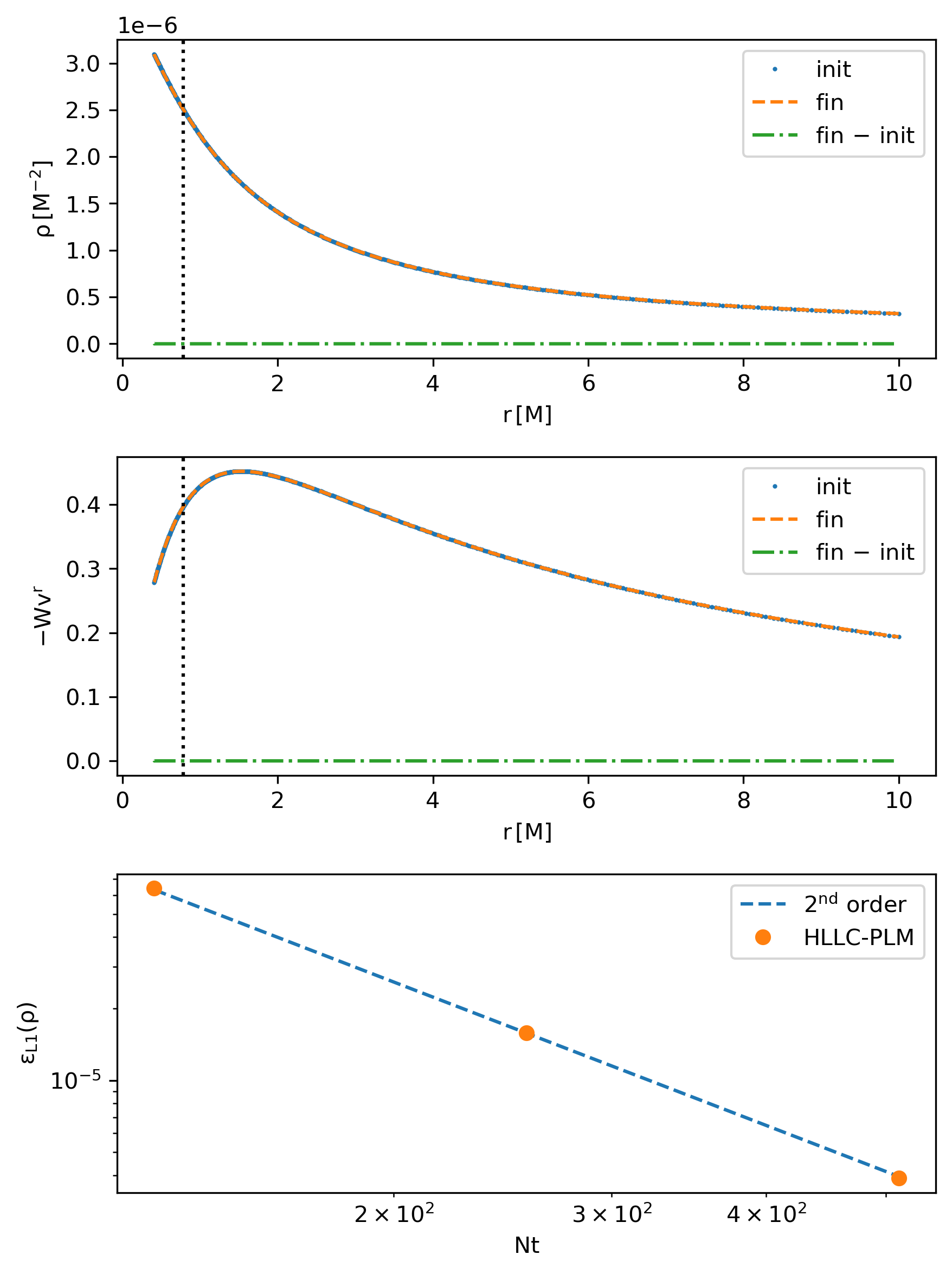
Figure 1: Top: radial rest-mass density profile of the Bondi flow for the medium resolution $\texttt{Nt}=256$ (Nt is the number of cells in the azimuthal direction). The mass accretion rate is $\dot{M}_{\rm{bondi}}=10^{-4}\,M$. The blue dotted line indicates the initial analytical solution at $T=0\,M$, while the yellow dashed line denotes the numerical solution at $T=50\,M$. The green dash-dotted line shows their difference. The black dotted vertical line indicates the radial location of the event horizon of the black hole at $r=0.7793\,M$ in the isotropic trumpet coordinate. The inner and outer boundaries of the simulation domain are $r=0.4\,M$ and $r=10\,M$, respectively. Middle: the radial fluid velocity $-Wv^{r}$ profile. $W$ is the Lorentz factor, $v^{r}$ is the fluid velocity with respect to the Eulerian observer. Bottom: the L1-norm of error for the rest-mass density as a function of the azimuthal grid number Nt. The dash line indicates 2nd-order convergence.

We first consider spherically symmetric, radial fluid accretion onto a non-rotating black hole (in-going Bondi flow) [100, 101]. Following previous work (e.g. [102, 71]), we perform simulations of Bondi flow in maximally sliced trumpet coordinates [103, 104]. The transformation between Schwarzschild coordinate and maximally slicing trumpet coordinate is illustrated as a reference in Appendix B. We set the fluid parameter according to table 1 of [102]: the accretion rate $\dot{M}_{\rm{bondi}}=10^{-4}M$, the adiabatic index $\Gamma=4/3$, the critical radius $R_{s}=10M$ where M is the mass of the central black hole. For simplicity, $M$ is set to 1 in the simulation.

The simulation domain is in an axisymmetric spherical coordinate, spanning the region $r\in[0.4\,M,10\,M],\ \theta\in[0,\pi/2]$. We employ logarithmic grid spacing in the radial direction with a cell’s aspect ratio $a$ set to one (i.e. $a:=\Delta r/r\Delta\theta=1$). The finest cell, located closest to the inner boundary, has a spacing $\Delta r=r_{\rm{min}}\,(\theta_{\rm{max}}-\theta_{\rm{min}})/(\texttt{Nt})$, where Nt is the number of cells in the azimuthal direction. To maintain the unity aspect ratio of the cell, the number of cells in the radial direction Nr is calculated as

$$\texttt{Nr}=\frac{\log(r_{\rm{max}}/r_{\rm{min}})}{\log(1+(\theta_{\rm{max}}-\theta_{\rm{min}})/\texttt{Nt})}.$$ (98)

We conduct simulations with three different resolutions: Low resolution with $\texttt{Nt}=128$, Medium resolution with $\texttt{Nt}=256$, and High resolution with $\texttt{Nt}=512$. For the benefit of convergence test, we set the number of grids in the radial direction $\texttt{Nr}=2\,\texttt{Nt}$. In this case, the cell’s aspect ratio will deviate from one slightly.

In Fig. 1, we show the radial profiles of the fluid rest-mass density (top) and the fluid velocity (middle) at time $T=0\,M\,(\rm{init})$ and $T=50\,M\,(\rm{fin})$ for the medium resolution simulation. The profile of the Bondi flow has been maintained throughout the simulations. In the bottom panel, we plot the L1-norm of error for the rest-mass density. The L1-norm of error is defined as [70]

$$\epsilon_{\rm L1}(\rho)=\frac{\int|\rho_{\rm{fin}}-\rho_{\rm{init}}|\sqrt{-g}drd\theta d\phi}{\int|\rho_{\rm{init}}|\sqrt{-g}drd\theta d\phi}.$$ (99)

The Bondi simulations demonstrate second-order convergence for the L1-norm of error with respect to the resolution. The code adopts the second-order RK2 time integrator and the second-order piece-wise linear reconstruction method (PLM), described in section IV.3. The presented convergence result is as expected and agrees with previous studies (see e.g. [70, 71]). For the implementation of a higher order reconstruction scheme for our unstructured grid in spherical geometry, like the piece-wise parabolic method “PPM” [105], weighted essentially non-oscillatory “WENO” [106, 107, 108, 109] or the monotonicity preserving scheme “MP5” [108], we will refer to future work.

V.2 Tolmann-Oppenheimer-Volkoff star

The next numerical test we consider is the Tolman–Oppenheimer–Volkoff (TOV) star with the structure of a spherically symmetric body of isotropic material in equilibrium [110, 111].

Table 1: Parameter values for the initial profile of TOV star.

Radius [km]	Gravitational mass $[M_{\odot}]$	Baryon mass $[M_{\odot}]$	$\rho_{c}\ [\rm{g/cm^{3}}]$
12	1.400	1.506	$7.92\times 10^{14}$

We conduct two TOV star tests based on[61]: the stationary case and the one with pressure depletion. The initial profile for the TOV star has a central rest mass density $\rho_{c}(0)=1.28\times 10^{-3}$. We adopts the polytropic EOS $P(\rho)=K\rho^{\Gamma}$, with $(K,\Gamma)=(100,2)$ for the initial data. As for the evolution, we adopt the ideal gas law. Additional parameters for the initial profile can be found in Table 1 in the cgs unit. In Fig. 2, we plot the central maximum density variation as a function of dynamical time ($\sqrt{\rho_{c}(0)}\,t$) for both cases. For the stationary case, we find the central maximum density varies within 0.3% for 14 dynamical times, confirming the stability of the star. When we reduce the initial pressure profile by 10 percent, the TOV star falls out of equilibrium and undergoes radial oscillations. We conduct simulations with two different resolutions ($\texttt{Nt}=64$ and $128$) and find consistent results, as shown in the bottom panel of Fig. 2. The oscillation pattern is equivalent to the test result in [61].

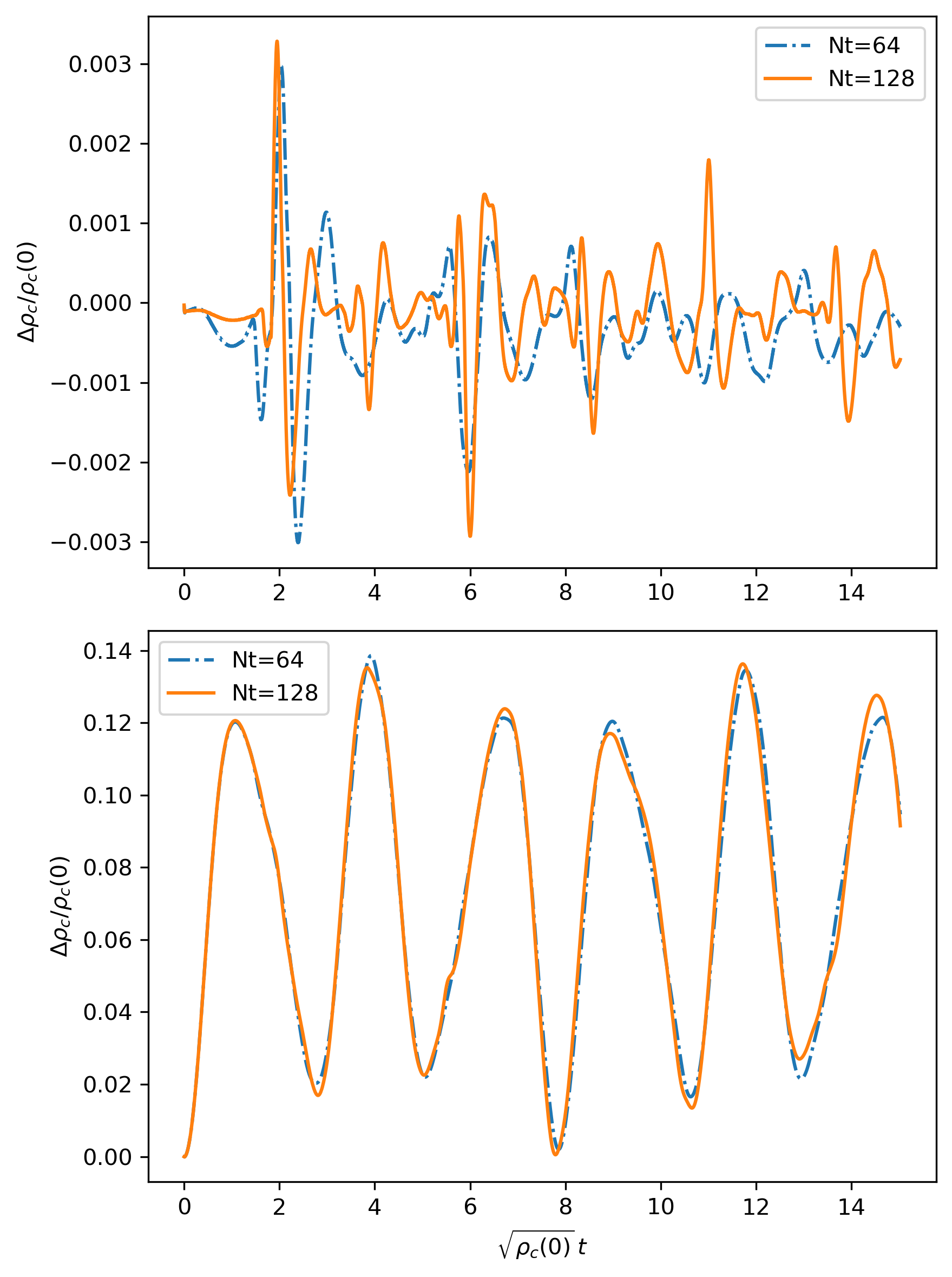
Figure 2: Normalized variation for the central maximum density as a function of dynamical time for the TOV star at two resolutions ($\texttt{Nt}=64$ and $\texttt{Nt}=128$). Top: the time evolution for the stationary case. Bottom: the time evolution for the pressure-depleted star whose equilibrium pressure has been reduced by 10 percent globally.

V.3 Fishbone-Moncrief torus around a Schwarzschild black hole

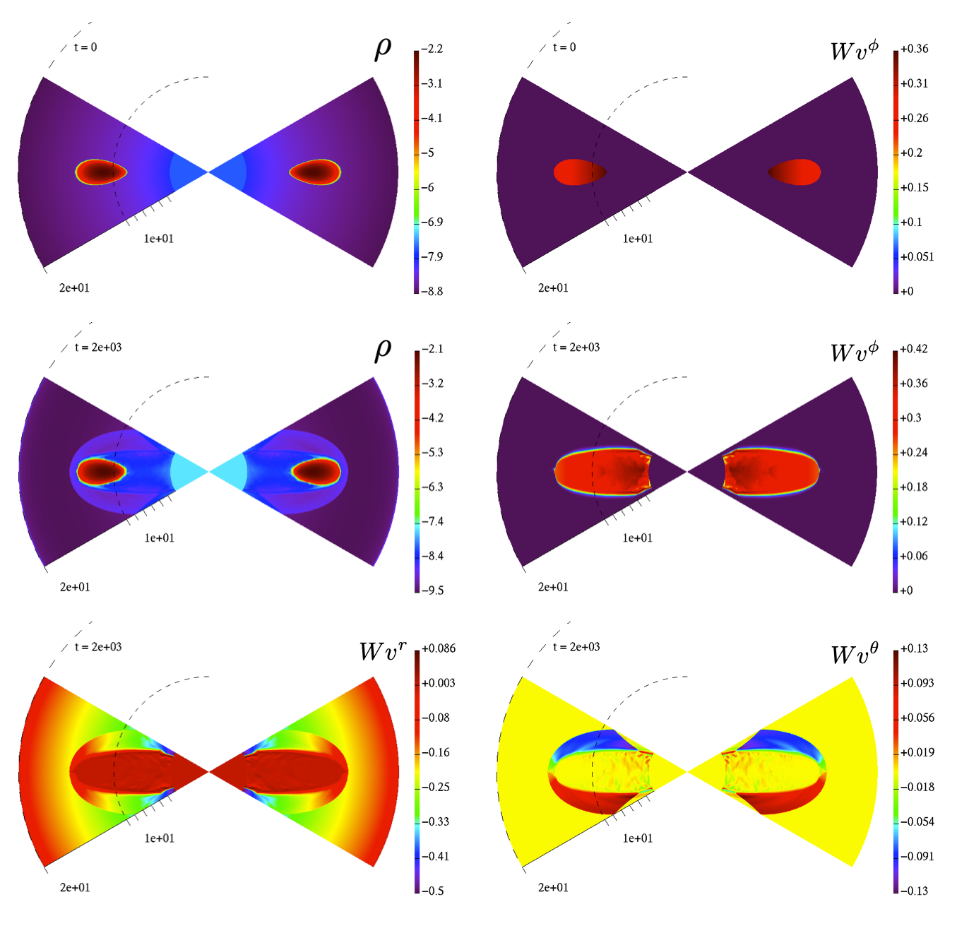
Figure 3: Contour plot of a stationary torus around a static black hole. The simulation adopts an axisymetric spherical domain. The azimuthal angle extends from $\pi/3$ to $2\pi/3$. The radial grid extends from $r_{min}=4$ to $r_{max}=20$. The top panel shows the initial profile of the logarithmic density (left) and the angular velocity $Wv^{\phi}$ (right), $W$ is the Lorentz factor of the flow. The middle panel represents the profile at the end of the simulation $t=2000$. The bottom panel represents the contour plot of the radial velocity $Wv^{r}$ (left) and the azimuthal velocity $Wv^{\theta}$ (right).

Our next test concerns a stationary, axisymmetric, isentropic torus around a Schwarzschild black hole [112]. We consider a particular instance of the Fishbone-Moncrief solution where the spin of the black hole is set to zero.

We generate the initial data in the Schwarzschild coordinate with its radius denoted by $R$. However, we will evolve the system in an isotropic trumpet coordinate of Schwarzschild metric with its radius denoted by $r$. The transformation between these two coordinates is illustrated in Appendix B. The initial profile generator follows the implementation in [87, 113, 80]. Table 2 shows the key variable values for the torus. For the ambient atmosphere, we set $\rho=\rho_{\rm{min}}(R/R_{g})^{-3/2},P=P_{\rm{min}}(R/R_{g})^{-5/2}$, where $\rho_{\rm{min}}=10^{-8},P_{\rm{min}}=10^{-10}$, $R_{g}=GM/c^{2}$ is the black hole gravitational radius and $M$ is the black hole mass.

Table 2: Parameters for the stationary torus around a black hole

$M~{}[M_{\odot}]$	$R_{\rm{in}}$	$R_{\rm{max}}$	$v^{\phi}_{\rm{max}}$
1	6	12	$2.893\times 10^{-1}$
$\rho_{\rm{max}}$	$l$	$\kappa$	$\Gamma$
$6.857\times 10^{-3}$	4.619	$1\times 10^{-3}$	4/3

For the simulation, we employ an ideal gas EOS: $P=(\Gamma-1)\rho\varepsilon$, with $\Gamma=4/3$. In azimuthal direction, the simulation domain extends from $\theta_{\rm{min}}=\pi/3$ to $\theta_{\rm{max}}=2\pi/3$. In the radial direction, the grid covers the region from $r_{\rm{min}}=4$ to $r_{\rm{max}}=20$. At the location of maximum pressure $r=10.98\,(R=12)$, the orbital period of the torus is around $238.1$. We set the final time of the simulation to be $2000$, roughly 9 orbits. We conduct two simulations with grid resolution $\texttt{Nt}=256$ and $\texttt{Nt}=512$, and find consistent results. In the following, we present the result from the $\texttt{Nt}=512$ simulation for better visual effect.

Figure 3 illustrates the contour plots of the black hole-torus system at the beginning (top panel) and at the end of the simulation (middle and bottom panels). The top panel shows the initial contour plot for the logarithmic density $\rho$ (left plot) and the angular velocity $Wv^{\phi}$ (right plot). Comparing these two contour snapshots, we first find that throughout the simulation, the torus maintains its density structure. The ambient gas falls into the black hole and blows the torus surface in the in-falling process. A bow shock appears in front of the torus and a trailing tail fills in the inner region between the torus and the central black hole. The small amount of gas, filling the space between the torus and the black hole, has minimal radial and azimuthal velocity (see the contour plot of the radial velocity $Wv^{r}$ and the azimuthal velocity $Wv^{\theta}$ in Fig 3). However, its angular velocity remains relatively high, indicating they are coming from the torus and rotating around and drifting towards the black hole. The stability of the black hole-torus system showcases the code’s robustness in the handling of fluid rotation under strong gravity.

V.4 Rayleigh-Taylor instability for a modified Bondi flow

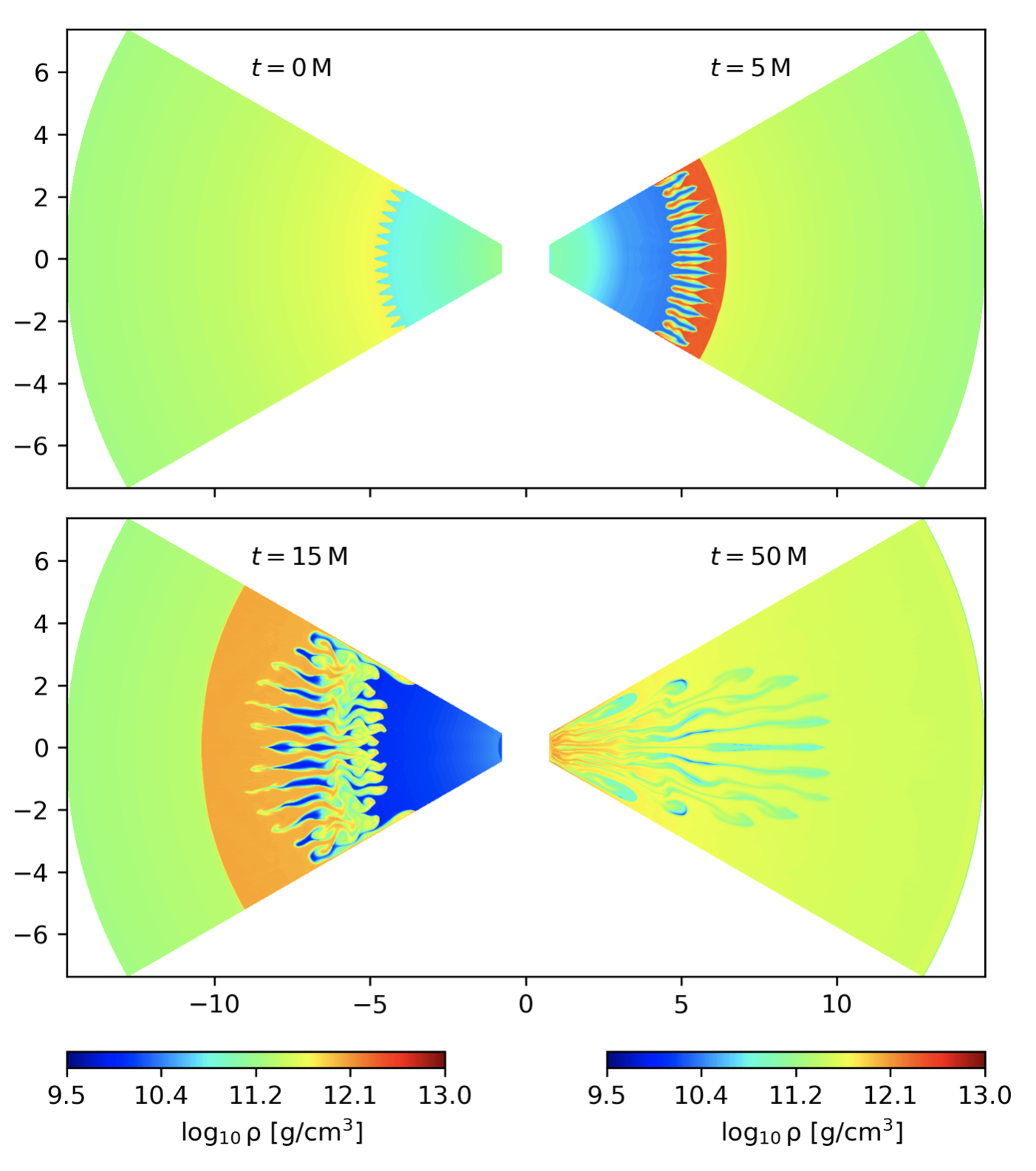
Figure 4: Time snapshots for the development of Rayleigh-Taylor instability of a hot low-density bubble embedded inside a cold Bondi flow. The contour plots represent the density of the flow. The simulation video is available from Youtube at https://youtu.be/71ZVnp05Xv4.

Previous work [58] with the original JET code has captured the detailed nonlinear features of Rayleigh-Taylor instability in a relativistic fireball. It uses the HLLC Riemann solver described in [56]. To test our general relativistic HLLC Riemann solver, we modify the Bondi flow to induce Rayleigh-Taylor instability under strong gravity. The setup is similar to a Strömgren sphere around the central black hole - the low-density hot gas is surrounded by a high-density gas with gravitational acceleration [114]. Within a radius of $r<3(1+0.1\times(1+\cos(80\theta))/2.0)$, the density and pressure of the Bondi flow have been modified as $\rho=0.1\rho_{\rm{bondi}},P=50P_{\rm{bondi}},v^{r}=0$. $\rho_{\rm{bondi}}$ and $P_{\rm{bondi}}$ is taken from the bondi profile in section V.1. This setup creates a hot low-density bubble inside the Bondi flow with a curly interface. As the hot low-density gas pushes against the heavier Bondi flow, Rayleigh-Taylor instability (or sometimes referred to as Richtmyer Meshkov instability in this case) develops. We perform this simulation with an azimuthal resolution of Nt=512, covering azimuthal angle from $\pi/3$ to $2\pi/3$. Figure 4 shows its time evolution. Initially, the hot gas pushes outward and compresses the incoming Bondi flow into higher density as shown at $t=5\,\rm{M}$. Instability fingers develop and evolve inside the low-density region. Nonlinear features of the instability continuously evolve at $t=15\,\rm{M}$. Later on, due to the attraction of the central black hole, the turbulent gas flows into the black hole. The implemented HLLC Riemann solver is able to capture the detailed structure of the instability in strong field regime.

VI Moving-Mesh Numerical Simulations

VI.1 Spherical shock tube test

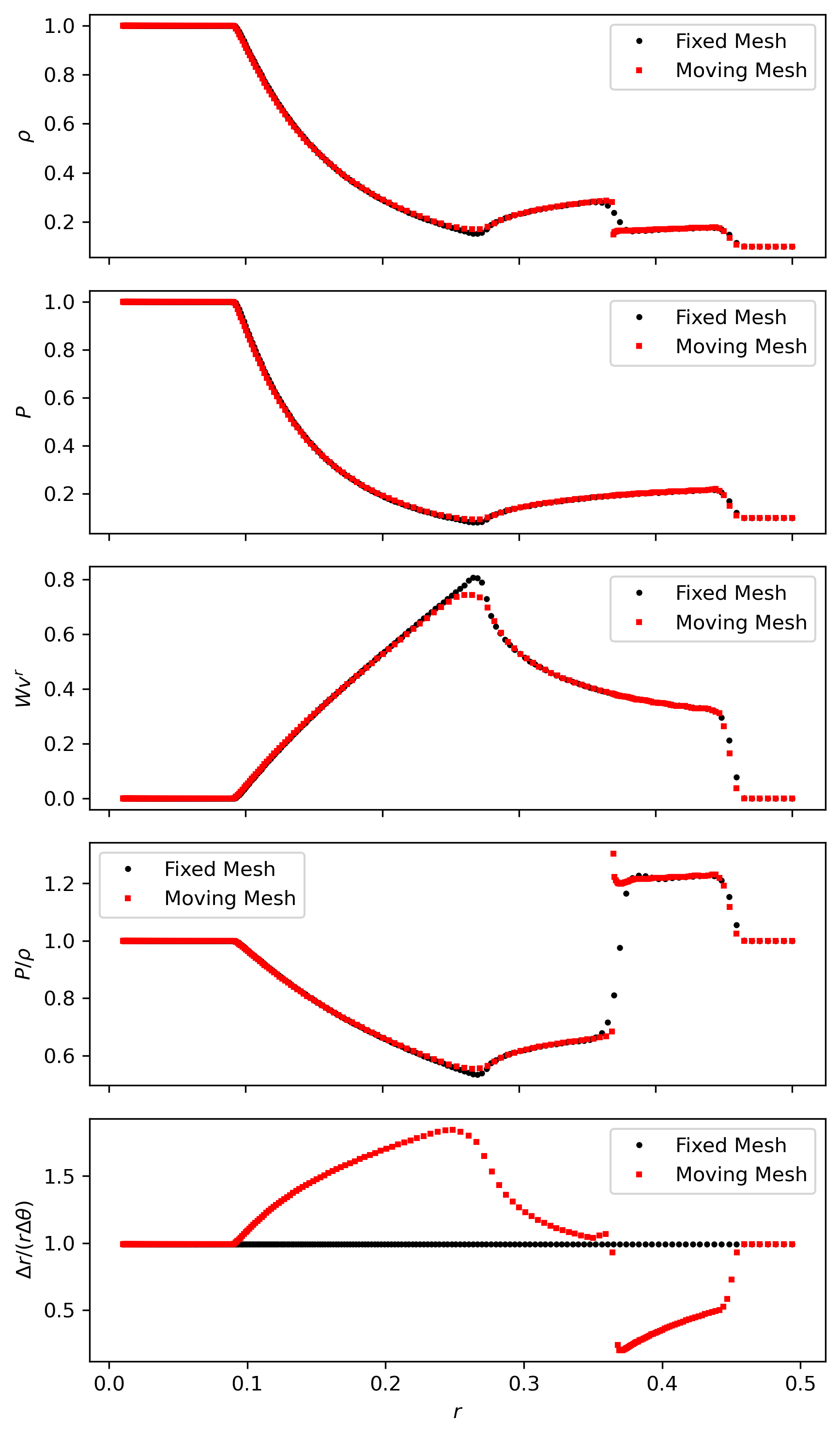
(a)

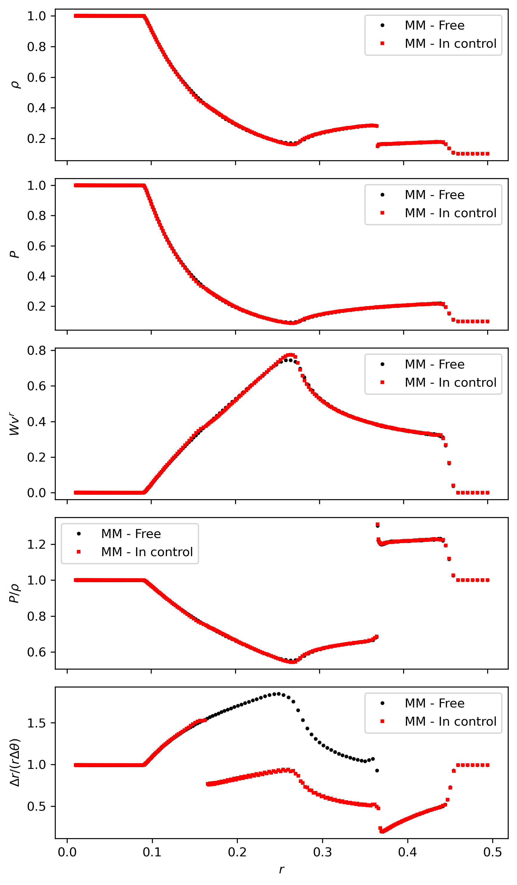
(b)

Figure 5: (a) Shock tube test in spherical coordinate for the fixed-mesh (black-dot) and moving-mesh (MM) (red-square) simulation. The profiles are presented at $t=0.3$. Initial discontinuity locates at $x=0.25$. The inner (outer) state of the shock tube is $\rho=1,P=1,v=0$ ($\rho=0.1,P=0.1,v=0$). The EOS follows the ideal gas law with $\Gamma=4/3$. (b) Shock tube test in spherical coordinate for the moving-mesh simulations with different control schemes for the cell’s aspect ratio. The black-dot line represents the simulation where the cell’s maximum aspect ratio has not been set. The red-square line shows the simulation where the maximum aspect ratio of the cell has been set to 1.5.

One advantage of our moving-mesh code is that the cell face is able to move with the contact velocity of the flow in the radial direction. It has been shown that the contact discontinuity is much better preserved when employing HLLC on the moving mesh(see Fig. 7 of [56]). What’s more, the flow naturally adjust the cell width in the radial direction. Combined with robust refinement and derefinement scheme, the simulation domain will be able to resolve the region of interest [65]. To test the accuracy of the moving-mesh scheme, we conduct the identical spherical shock tube test as shown in [62]: within the radius of 0.25 ($r<0.25$), the density $\rho$ and pressure $P$ is set to 1. Outside of this region, the value of density and pressure is 0.1. We adopt the Minkowskian frame for the test. Since the tetrad formulation for the HLLC Riemann solver also works for the Minkowskian metric, we do not take any additional steps for the special relativistic simulations.

In azimuthal direction, the simulation domain extends from 0 to $\pi/2$ with $\texttt{Nt}=128$. In the radial direction, the grid covers the region from $r_{\rm{min}}=0.01$ to $r_{\rm{max}}=0.5$. We adopt logarithmic spacing in the radial direction and set the initial cell’s aspect ratio to one. In Fig. 5a, we show the profile comparison at the end of the simulation with fixed mesh setup and moving mesh setup. The density plot exhibits a sharp transition at the contact discontinuity for the moving mesh and a relatively smooth one for the fixed mesh. Following the compression of the fluid in the shocked region, the cells squeeze between the contact discontinuity and the forward shock. The $P/\rho$ plot reveals a jump at the contact discontinuity. We find this appears in the moving-mesh simulation here as well as in the literature [56, 62]. It may come from the squeezing of the fluid as the grid moves along or the TVD reconstruction scheme requires some adjustification for the moving-mesh. Since the jump does not grow with time and has minimal impact on the fluid dynamics, we will leave this numerical phenomena to the research community for now. In the rarefaction region, the cells get elongated, leading to an aspect ratio larger than one. Because of the increase in the aspect ratio (i.e. the reduction of radial resolution), we find the peak of the velocity profile for the moving-mesh simulation becomes less sharp compared to the fixed mesh simulation.

However, since we have full control over the grid refinement, we can specify the maximum aspect ratio in the simulation. We conduct another moving mesh sod-tube simulation which sets the maximum aspect ratio to 1.5. When the elongated cell reaches such a threshold, it will split into two cells. To show the effect of such a refinement scheme on the sod-tube simulation, we compare the profiles for the moving-mesh simulation with or without maximum aspect ratio control in Fig. 5b. With the maximum aspect ratio control, the resolution in the region where the cell’s aspect ratio gets to the threshold value increases. The peak of the velocity profile becomes sharper compared to the peak for the moving-mesh simulation without aspect ratio control. Overall, the implemented HLLC Riemann Solver on the moving-mesh is robust for simulating relativistic outflow.

VI.2 Relativistic jet emerged from a black hole-torus system

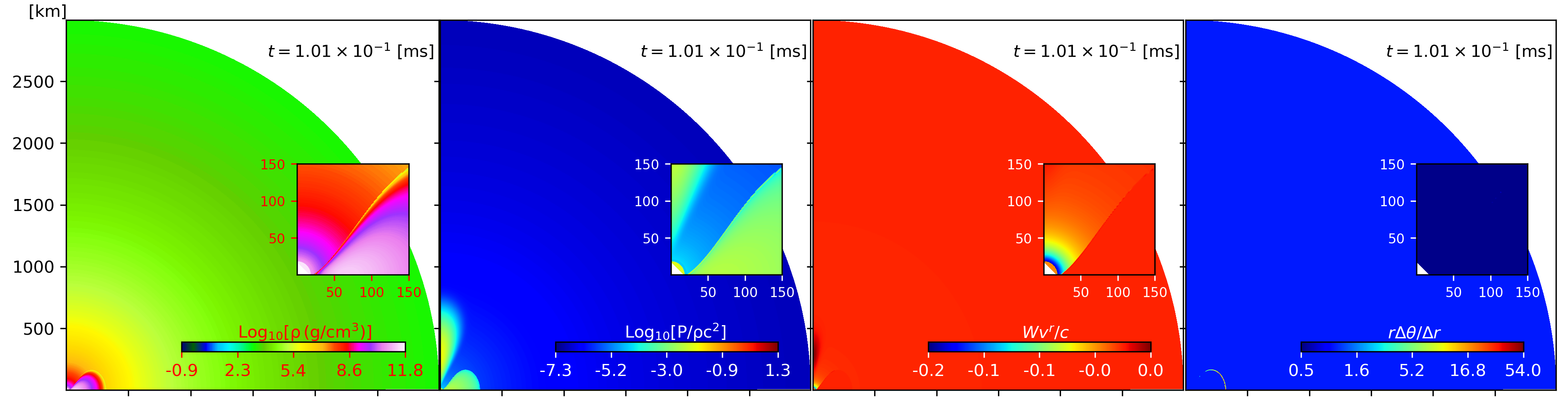
(a)

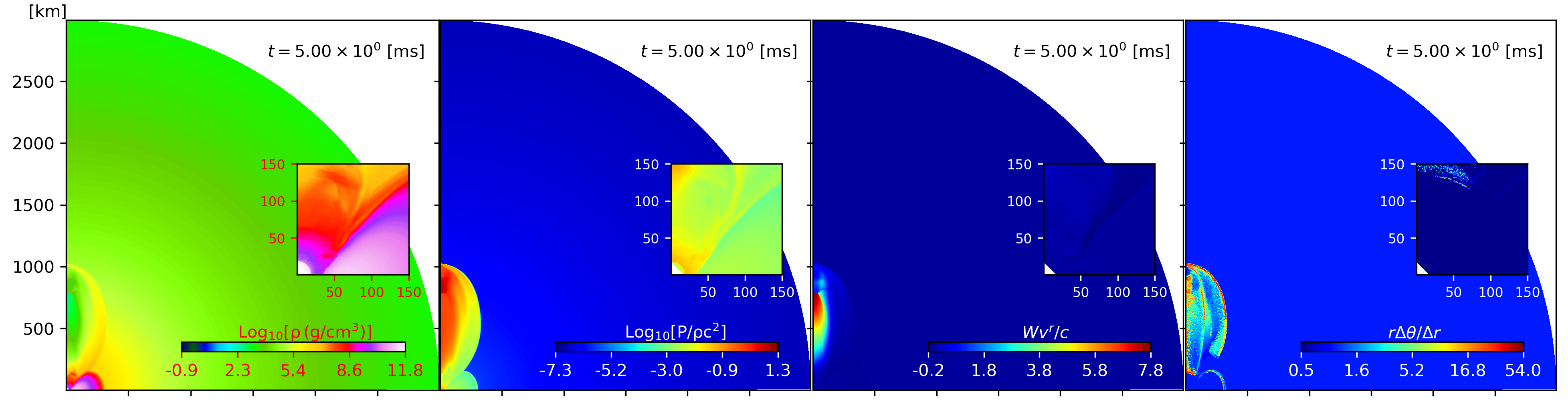
(b)

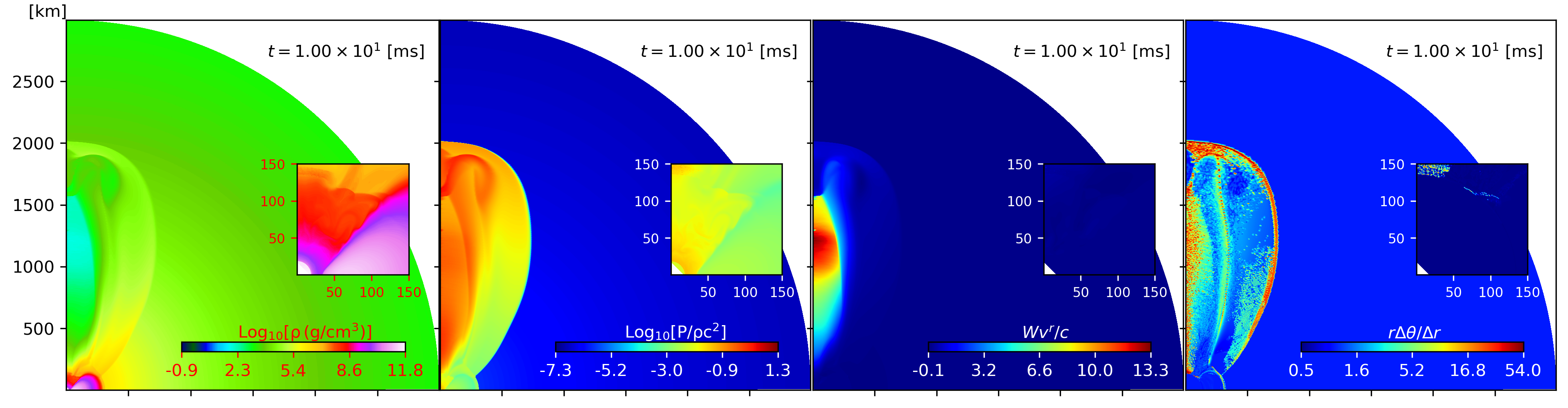
(c)

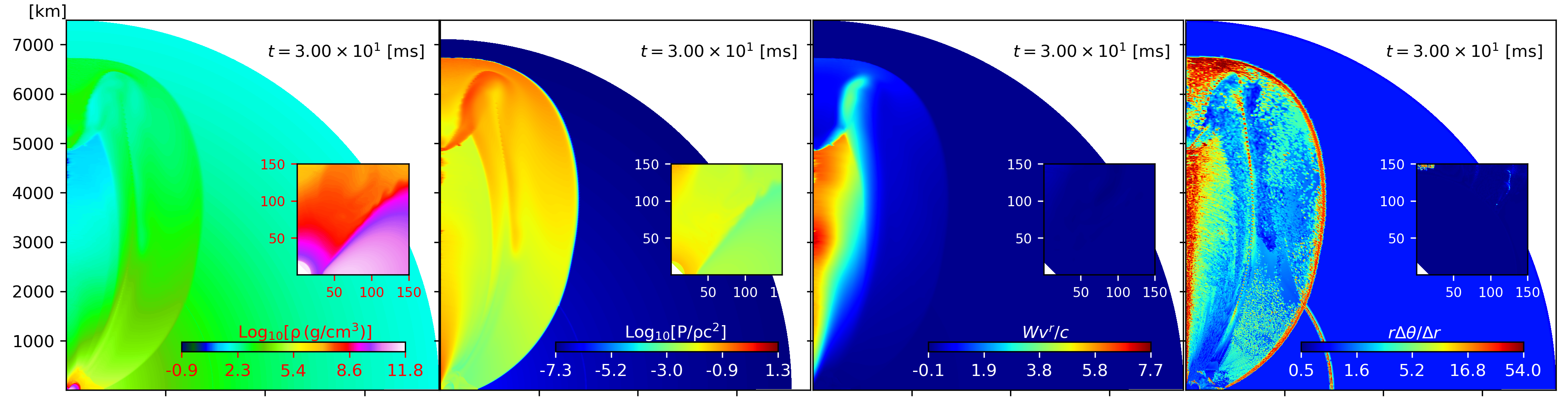
(d)

Figure 6: Jet launching process from a black hole-torus system, visualized at four-time snapshots. From left to right, the contour plots represent the logarithmic density, temperature-like variable $\Theta$, normalized radial velocity $Wv^{r}/c$, and the cell’s radial resolution (i.e. inverse aspect ratio). The inner contour plots zoom in on the central region of the domain. The inner boundary is stationary before $t=30\,\rm{[ms]}$. The simulation video is available from Youtube at https://youtu.be/JxXRlxhlwCs with 4K video quality available.

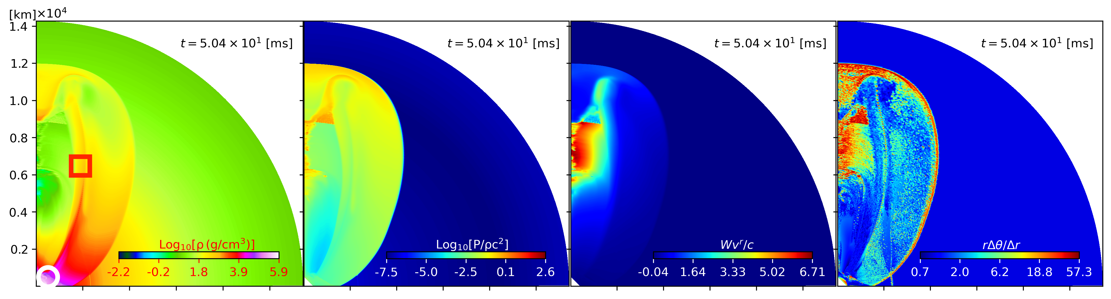
(a)

(b)

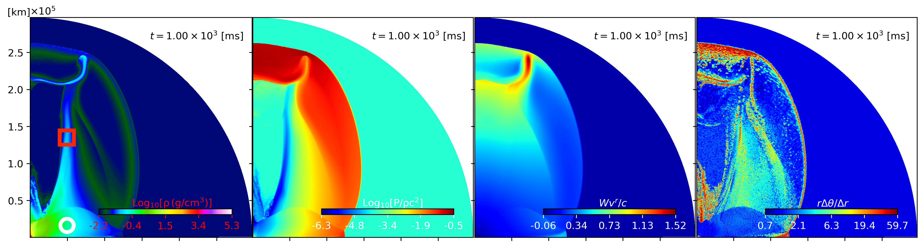
(c)

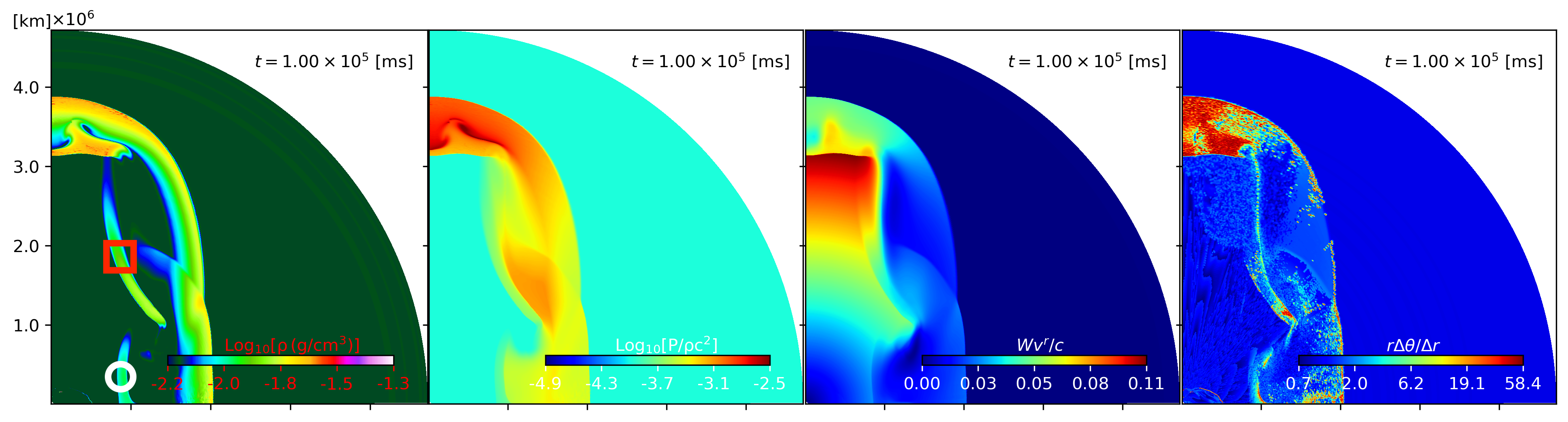
(d)

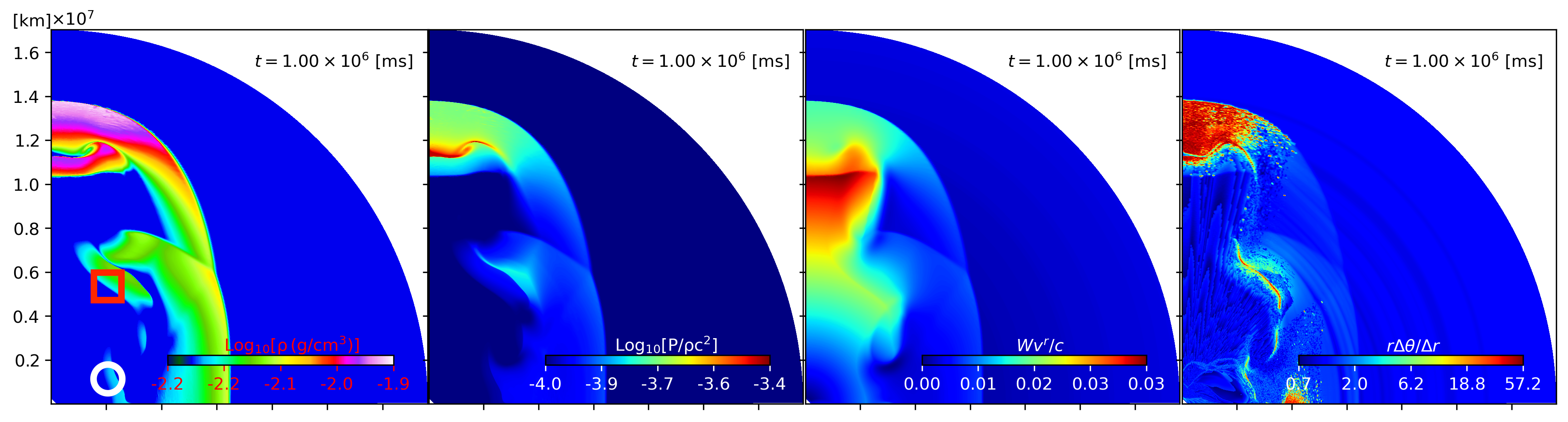
(e)

Figure 7: The full-time-domain evolution of the relativistic jet emerged from a black hole-torus system. The inner boundary moves outward at a fraction of the local maximum velocity. The simulation video is available from Youtube at https://youtu.be/JxXRlxhlwCs with 4K video quality available.

The detection of the gravitational wave (GW) signal GW170817, coupled with the observations of its electromagnetic (EM) counterpart signifies the commencement of the multi-messenger astronomy era [115]. Research has demonstrated that the structure of the emerged relativistic outflows plays a crucial role in shaping the afterglow emission in GRB170817A [116, 52, 117, 118, 119, 120, 121, 122]. This event provides an ideal candidate for utilizing the electromagnetic observations of the emerged outflow to infer the BNS merging physics. While the presented moving-mesh code is capable of simulating relativistic jets out of various progenitor systems, in the following, we will use a pseudo-model inspired by the outcome of BNS merger simulations (see e.g., [123]). We set up a black hole-torus system in an isotropic coordinate of Schwarzschild metric, with the mass of the central black hole $M$ been set to $M=3M_{\odot}$ and the torus mass been set to $0.2\,M_{\odot}$. The radius of inner edge of torus is $6\,M$, and the radius of its pressure maximum is set to $16\,M$ [124]. For the simulation domain, the radius of inner boundary locates at $12$. And we use $\texttt{Nt}=256$ grids to cover the half spherical domain with cell’s initial aspect ratio been set to 1. We adopt reflecting boundary condition in the azimuthal direction. Outside the torus, the domain is filled with an ejecta cloud with a total mass of $0.02\,M_{\odot}$. The cloud density structure follows:

$$\rho=\rho_{0}(r/r_{0})^{-n}+\rho_{\rm{floor}}.$$ (100)

$\rho_{0}=(n-3)M_{\rm{ejecta}}/(4\pi r_{0}^{3})$ is derived to give a total ejecta mass $M_{\rm{ejecta}}$. The pressure is $P=K\rho^{\Gamma}+P_{\rm{floor}},K=0.54,\Gamma=4/3$. We also add a density floor $\rho_{\rm{floor}}=6.2\times 10^{-5}\,\rm{[g/cm^{3}]}(\,\rm{i.e.}\,10^{-22}\rm{\ in\ the\ code\ unit})$ and a pressure floor $P_{\rm{floor}}=10^{-4}\rho_{\rm{floor}}$ to the initial profile to avoid numerical precision error. We set the density slope index $n=3.5$ to represent the post-merger ejecta profile. Here, we ignore the ejecta profile velocity for simplicity. The reference radius $r_{0}$ is set to $6M_{\odot}$. A jet engine with a variable luminosity of $L_{0}=2\times 10^{51}\,\rm{exp}(-t/t_{\rm{decay}})\,[\rm{erg/s}]$ operates for $30\,\rm{ms}$, in the polar region just above the black hole-torus plane. The engine decay time scale $t_{\rm{decay}}$ has been set to $100\,\rm{ms}$. This gives a total injected jet engine energy $5.2\times 10^{49}\,[\rm{erg}]$. We choose this low-energy jet engine injection to test the code’s capability of launching a relativistic jet under constraint. In jet simulations, it becomes easier to successfully launch a relativistic jet given a higher energy injection (see e.g. [52, 65]). The profile of the jet engine features a narrow nozzle with an opening angle of $0.1\,\rm{rad}$. For the complete jet engine profile, we refer readers to the description in Appendix C as well as in [65, 64].

Figure 6 shows the jet launching process during the first $30\,\rm{ms}$. At the beginning of the simulation, the cloud flows into the black hole. In the polar direction, at a location centered around $130\,[\rm{km}]$, a small amount of relativistic gas with a terminal Lorentz factor 100 (i.e. jet engine) gets injected into the cloud. The injected gas has an initial boost velocity in the radial direction (see Appendix C). The addition of the relativistic gas slightly pushes the cloud gas in the polar direction, leading to a non-negative radial velocity (as can be seen from the radial velocity plot at $t=0.1\,[\rm{ms}]$). The continuous injection of hot relativistic gas drives shocks and changes the temperature profile in the polar direction. By the time $t=5\,[\rm{ms}]$, a shocked cocoon develops and reveals a two-laryer structure: a high-density layer which results from the forward shock, meanwhile the inner cocoon which heats up by the jet engine and reverse shock gets to a low-density regime [125, 126, 42]. Inside the inner cocoon, the shocked gas accelerates to a high velocity with a maximum Lorentz factor around 8 at $t=5\,[\rm{ms}]$. The moving mesh scheme dynamically allocates cells to resolve the shocked region. The interfaces of the double-layer structure can be seen in the contour plot for the cell’s radial resolution: the first interface lies in the shock front between the cocoon and the unperturbed cloud, the second interface is between the cocoon’s inner low-density hot relativistic core and its high-density colder part. At the bottom of the cocoon, the shock front hits the torus. At $t=10\,[\rm{ms}]$, the shock front starts to move beyond the torus and wrap around it. At the head of the cocoon, the loaded matter diverts part of the shocked gas sideways. Below this region, the inner core of the cocoon accelerates to a higher Lorentz factor of 13. Throughout the acceleration period, the maximum Lorentz factor of the jet reaches $20$ (which happens at about $t=13\,[\rm{ms}]$), smaller than the terminal Lorentz factor of the injected relativistic gas. This is largely due to the engine’s relative low-energy budget (we refer readers to more energetic jet simulations in [52, 65]). By the end of the jet engine injection $t=30\,[\rm{ms}]$, at the base of the grid domain, the frontier of the shocked cocoon has passed the torus region. A relative high density buffer zone appears between the torus and the cocoon (see the density and temperature contour plots). The torus itself rotates stably during the jet launching process, as illustrated by the inner contour plots in Fig. 6. The head of the shocked cocoon expands beyond the initial grid domain boundary. More cells will be allocated in front of the boundary as the shock front propagates. The radius of the new boundary will make sure that the head of the shock front will stay below 0.8 of this new radius during the simulation.

Figure 7 illustrates the continued evolution of the relativistic cocoon that emerged from the black hole-torus system when the jet engine had been turned off. For computational efficiency, we cut the grid domain within a radius of $300$ (around $440\,[\rm{km}]$). We let the inner boundary move with a velocity of a fraction of the fluid’s local maximum velocity. With the inner and outer boundary expands outward together, the simulation gets into a (weak) scaling region where the simulation time step $\Delta t$ increases with the absolute time itself. In this way, the moving-mesh code in spherical coordinates can simulate long-term evolution of relativistic jets over multiple orders of magnitude of time. When the jet engine turns off, it stops accelerating nearby gas. The inner cocoon turns into a shrinking relativistic bubble. The relativistic bubble keeps pushing against the mass-loaded head, exhausting its internal energy and kinetic energy. By the time $t=50\,[\rm{ms}]$, the top of the bubble starts to decelerate dramatically. The collision with the mass-loaded head converts part of its kinetic energy into thermal energy. The collision drives a wave passing through the relativistic bubble, increasing the temperature of inner cocoon all the way to its bottom (see the simulation video). Eventually, the relativistic bubble turns into a relativistic thin shell (see the velocity contour at $t=300\,[\rm{ms}]$). The relativistic shell features a relativistic core with a mildly relativistic sheath, similar to previous special relativistic jet simulations (see e.g. [123, 127, 52, 65]). The outer layer of the cocoon goes through adiabatic expansion. The density within this layer keeps decreasing while the temperature structure roughly remains the same (see the contour plots for the temperature-like variable from $t=50\,\rm{[ms]}$ to $t=1\,\rm{[s]}$.). The interface between the inner and outer cocoon features a high density pillar. The relativistic shell keeps sweeping through the medium while depleting its kinetic energy. By the time $t=100\,s$, the relativistic thin shell is replaced by a mass-loaded slow-moving core. We see a morphological change in the outer shell structure. Finally, by the end of our simulation $t=1000\,s$, the outflow velocity becomes completely Newtonian. Now we have seen the complete life cycle of a relativistic jet from its birth at a black hole scale to the distance of its dissipation. In the following, we would like to discuss two dynamical features for this specific simulation. The first feature of interest focuses on the base of cocoon. In Fig. 7, we use white circle to indicate this region of interest. We find it appears after the shock front of the cocoon passed over the torus. It originates from the buffer zone or shock zone between the original torus and the remaining cocoon. It propogates subrelativistically and maintains its hump shape before $t=1\,\rm{[s]}$. Later on, the shock front accumulates enough matter and slows down to Newtonian velocities. When this happens, via hydrodynamical interaction, the morphology of the region changes and the hump shape disappears, leaving behind a broken filament as shown at $t=100\,s$ and $t=1000\,s$. The second feature of interest relates to the density pillar at the interface between the inner and outer cocoon. We mark it with red square in the figure. Its formation, to some extent, comes from the shutdown of the central jet engine during the jet launching period. At the beginning, when the central jet engine inflates a cocoon, it drives mass and energy into the cocoon outer layer while creates a low-density hot inner funnel to generate relativistic outflow. When the central engine shuts down, the inner cocoon quickly gets cold and stops pushing the outer layer (see snapshots at $t=50\,\rm{[ms]}$ and $t=300\,\rm{[ms]}$). Then the adiabatic expansion of the outer layer further separates this interface from the shock front as shown at $t=1\,\rm{[s]}$. The interface pillar also has positive radial velocity and moves with the outer shell. However, the part, connecting to the outer shell, moves faster. To a point, the pillar detaches itself from the outer shell and falls back to the inner region. This is what happens from $t=100\,\rm{s}$ to $t=1000\,\rm{s}$. Because of the long-term simulation of the relativistic jet, we are able to capture such detailed hydrodynamics evolution, which may provide insights for the study of morphologies of astronomical jets. Throughout the simulation, the maximum grid resolution in the radial direction remains below 60 - a value we set initially.We see that the moving-mesh scheme, combined with the dynamical grid refinement and derefinement can capture the detailed dynamical features for the relativistic jet simulation over many orders of magnitude of space and time.

VII Conclusion

This paper presents an advancement in computational astrophysics: developing and implementing a general relativistic moving-mesh hydrodynamic code featuring an advanced Riemann solver in curvilinear coordinates. We showcase the details of integrating a general relativistic framework into the hydrodynamic simulation code- JET, achieved through applying the reference metric method.

At the heart of this work is utilizing the tetrad formulation to address the Harten, Lax, and van Leer Contact (HLLC) Riemann problem under strong gravity. With its ability to elegantly handle the intricate space-time geometries inherent in general relativity, the tetrad formulation is an ideal choice. A significant achievement of our work is the successful adaptation of the tetrad formulation for incorporating the HLLC Riemann solver into the general relativistic moving-mesh code. We have conducted a series of numerical simulations to validate and demonstrate the efficacy of our newly developed code. These simulations encompass both fixed-mesh and moving-mesh scenarios, allowing us to test the code’s performance under various conditions thoroughly. The results from these simulations are particularly noteworthy in demonstrating the code’s robustness and reliability in simulating fluid flows under the influence of strong gravitational fields.

Compared to the fixed-mesh approach, a moving-mesh scheme can increase the time step for fluid regions with high velocity since it removes the limitation imposed by the bulk velocity (see e.g. [62]). The moving-mesh approach makes the long-term simulation of relativistic jets computationally feasible (see e.g. [64, 52, 65]). By extending the JET code’s capability of handling relativistic jets from an astronomical scale to the scale of a black hole, we have opened new avenues for the full-time-domain simulation of relativistic jets, from their genesis to dissipation. To demonstrate this possibility, we design a representative prototype model which features a torus around a central black hole. A jet is manually launched in the polar direction, near the black hole-torus system. For the underlining jet launching mechanism, we refer readers to Blandford-Payne [4] or Blandford-Znajek [3] and related dynamo processes (see e.g.[11, 14]). In this work, we prescribe an engine profile to imitate the jet launching process. This setup allows us to explore the dynamics of the jet’s journey from its origin near the black hole-torus system to its final Newtonian phase. We found multiple new hydrodynamical feasures from this end-to-end simulation. For the first time, we have been able to simulate the complete life cycle of a relativistic jet, providing insights into the detailed structures of the cocoon and emerged jet over the whole jouney.

Furthermore, these full-time-domain jet simulations enables the joint investigation of various electromagnetic phenomena associated with relativistic outflows. For the case of BNS mergers, the observational phenomena include the kilo-nova emission from the remnant ejecta (see e.g. [26, 128, 27]), the sGRB prompt and afterglow emission (see e.g. [129, 130, 25]), and other related processes. By combining our simulations with general relativistic magnetohydrodynamic (GRMHD) models of jet-launching processes, we will be able to extend the evolution of outflows to distances relevant to long-term electromagnetic radiation observations. This integrative approach aligns perfectly with the era of multi-messenger astronomy, allowing for an unprecedented understanding of the underlying physics in jet-launching systems.

While this paper sets the foundational steps in this direction, the complete realization of these ambitious goals remains a pursuit for future research. The potential for further advancements and discoveries in the field is vast, and our work may catalyze the next generation of astrophysical jet simulations, potentially revolutionizing our understanding of relativistic jets and their associated physics.

Appendix A General relativistic hydrodynamic equations in reference metric formulation

A.1 The continuity equation

The covariant divergence of a vector $V^{\mu}$ gives

$$\nabla_{\mu}V^{\mu}=\frac{1}{\sqrt{-g}}\partial_{\mu}\left(\sqrt{-g}V^{\mu}\right),$$ (101)

which holds for any metric and its associated covariant derivative. The covariant divergence of a mixed-index second-rank tensor $A_{\mu}{}^{\nu}$, on the other hands, follows (see e.g. [75])

$$\nabla_{\nu}A_{\mu}{}^{\nu}=\frac{1}{\sqrt{-g}}\partial_{\nu}\left(\sqrt{-g}A_{\mu}{}^{\nu}\right)-A_{\xi}{}^{\nu}\Gamma_{\nu\mu}^{\xi}.$$ (102)

We will utilize these two rules to derive the general relativistic hydrodynamic equations.

Let us first apply Eq. (101) to the continuity equation (5)

$$0 =\nabla_{\nu}\left(\rho u^{\nu}\right)=\frac{1}{\sqrt{-g}}\partial_{\nu}\left(\sqrt{-g}\rho u^{\nu}\right),$$ (103)

$$=\frac{1}{\sqrt{-g}}\left(\partial_{0}\left(\sqrt{-g}\rho u^{0}\right)+\partial_{j}\left(\sqrt{-g}\rho u^{j}\right)\right).$$

The determinant of the space-time metric leads to

$$\sqrt{-g}=\alpha\sqrt{\gamma}=\alpha\psi^{6}\sqrt{\bar{\gamma}}=\sqrt{\hat{\gamma}}\alpha\psi^{6}\sqrt{\frac{\bar{\gamma}}{\hat{\gamma}}}.$$ (104)

Inserting the previous result into Eq. (103) we obtain

$$\partial_{0}\left(\psi^{6}\sqrt{\bar{\gamma}/\hat{\gamma}}D\right)+\frac{1}{\sqrt{\hat{\gamma}}}\partial_{j}\left[\sqrt{\hat{\gamma}}\left(f_{D}\right)^{j}\right]=0,$$ (105)

or sometimes written as

$$\partial_{0}\left(\psi^{6}\sqrt{\bar{\gamma}/\hat{\gamma}}D\right)+\hat{\mathcal{D}}_{j}\left[\left(f_{D}\right)^{j}\right]=0,$$ (106)

where $\hat{\mathcal{D}}_{j}$ is the covariant derivative with respect to the reference metric $\hat{\gamma}$. In the above expression, we have defined the density as seen by a normal observer as

$$D=W\rho,$$ (107)

and the corresponding flux

$$(f_{D})^{j}=\alpha\psi^{6}\sqrt{\bar{\gamma}/\hat{\gamma}}D(v^{j}-\beta^{j}/\alpha).$$ (108)

Note that, the fluid velocity as measured by a normal observer, $v^{i}$, is given by the ratio between the projection of the 4-velocity, $u^{\mu}$, in the space orthogonal to $n^{\mu}$ and the Lorentz factor of $u^{\mu}$ as measured by a normal observer, $W=-n_{\mu}u^{\mu}=\alpha u^{t}$:

$$v^{i}=\frac{\gamma^{i}_{\mu}u^{\mu}}{\alpha u^{t}}=\frac{u^{i}}{W}+\frac{\beta^{i}}{\alpha}.$$ (109)

A.2 The Euler equation

To derive the Euler equation, we apply Eq. (102) to the projected conservation of energy momentum (6)

$$0 =\gamma_{i\mu}\nabla_{\nu}T^{\nu\mu}=g_{i\mu}\nabla_{\nu}T^{\nu\mu}=\nabla_{\nu}\left(g_{i\mu}T^{\nu\mu}\right)$$ (110)

$$=\frac{1}{\sqrt{-g}}\partial_{\nu}\left(\sqrt{-g}T_{i}^{\nu}\right)-T_{\nu}^{\mu}\Gamma_{i\mu}^{\nu}.$$

We then get the following Euler equation

$$\frac{1}{\sqrt{-g}}\left(\partial_{0}\left(\sqrt{-g}T_{i}^{0}\right)+\partial_{j}\left(\sqrt{-g}T_{i}^{j}\right)\right)=T_{\nu}^{\mu}\Gamma_{i\mu}^{\nu}.$$ (111)

Note that the source term leads to

$$T^{\mu}_{\nu}\Gamma_{i\mu}^{\nu}=T^{\mu\xi}g_{\xi\nu}\Gamma^{\nu}_{i\mu}=\frac{1}{2}T^{\mu\xi}g_{\xi\mu,i}.$$ (112)

Let us define

$$\begin{split}T^{\mu\nu}&=\rho hu^{\mu}u^{\nu}+Pg^{\mu\nu}\\ &=S_{0}n^{\mu}n^{\nu}+S^{\mu}n^{\nu}+S^{\nu}n^{\mu}+S^{\mu\nu},\end{split}$$ (113a)

$$S_{0} =\rho hW^{2}-P,$$ (113b)

$$S^{i} =\rho hW^{2}v^{i},$$ (113c)

$$S^{ij} =\rho hW^{2}v^{i}v^{j}+P\gamma^{ij},$$ (113d)

and calculate the source term (112). The result is shown below (for the derivation, we refer readers to numerical relativity books [78])

$$\begin{split}\frac{1}{2}\sqrt{-g}T^{\mu\nu}g_{\mu\nu,i}&=\sqrt{-g}\left(\frac{1}{2}S^{jk}\partial_{i}\gamma_{jk}+S^{\mu}n^{\nu}\partial_{i}g_{\mu\nu}\right.\\ &\left.+\frac{1}{2}S_{0}n^{\mu}n^{\nu}\partial_{i}g_{\mu\nu}\right)\\ &=\sqrt{-g}\left(\frac{1}{2}S^{jk}\partial_{i}\gamma_{jk}+\frac{1}{\alpha}S_{j}\partial_{i}\beta^{j}-S_{0}\partial_{i}\ln\alpha\right).\end{split}$$ (114)

Let us define the momentum flux as

$$\left(f_{S}\right)_{i}{}^{j} \equiv\alpha\psi^{6}\sqrt{\bar{\gamma}/\hat{\gamma}}T_{i}^{j}$$ (115)

$$=\alpha\psi^{6}\sqrt{\bar{\gamma}/\hat{\gamma}}\left(W^{2}\rho hv_{i}\left(v^{j}-\beta^{j}/\alpha\right)+P\delta_{i}^{j}\right).$$

We can then rewrite the Euler equation (111) in the following form

$$\partial_{0}\left(\psi^{6}\sqrt{\bar{\gamma}/\hat{\gamma}}S_{i}\right)+\frac{1}{\sqrt{\hat{\gamma}}}\partial_{j}\left[\sqrt{\hat{\gamma}}\left(f_{S}\right)_{i}^{\ j}\right]=\left(s_{S}\right)_{i}.$$ (116)

The definition of the source term is given accordingly

$$(s_{S})_{i} =\frac{1}{2}\alpha\psi^{6}\sqrt{\frac{\bar{\gamma}}{\hat{\gamma}}}S^{jk}\partial_{i}\gamma_{jk}$$ (117)

$$+\psi^{6}\sqrt{\frac{\bar{\gamma}}{\hat{\gamma}}}S_{j}\partial_{i}\beta^{j}-\psi^{6}\sqrt{\frac{\bar{\gamma}}{\hat{\gamma}}}S_{0}\partial_{i}\alpha,$$

where the first term can be calculated as

$$S^{jk}\partial_{i}\gamma_{jk} =S^{jk}\partial_{i}\left(\psi^{4}\bar{\gamma}_{jk}\right)$$ (118)

$$=S^{jk}\gamma_{jk}\psi^{-4}\partial_{i}\psi^{4}+\psi^{4}S^{jk}\partial_{i}(\hat{\gamma}_{jk}+\epsilon_{jk})$$

$$=(\rho h(W^{2}-1)+3P)4\partial_{i}\ln\psi$$

$$+\psi^{4}S^{jk}\partial_{i}(\hat{\gamma}_{jk})+\psi^{4}S^{jk}\partial_{i}(\epsilon_{jk})$$

A.3 The energy equation

For the energy equation, we consider a projection along the normal $n_{\mu}$ of the conservation of energy-momentum (6) and add the conservation of rest mass (5)

$$n_{\nu}\nabla_{\mu}T^{\mu\nu}+\nabla_{\mu}\left(\rho u^{\mu}\right)=0,$$ (119)

which can be rewritten as

$$\nabla_{\mu}\left(n_{\nu}T^{\nu\mu}+\rho u^{\mu}\right)=T^{\mu\nu}\nabla_{\mu}n_{\nu}.$$ (120)

We again evaluate the divergence of a vector on the left-hand side, and proceed exactly the same as for the continuity equation, which leads to

$$\partial_{0}\left(\psi^{6}\sqrt{\bar{\gamma}/\hat{\gamma}}\tau\right)+\frac{1}{\sqrt{\hat{\gamma}}}\partial_{j}\left[\sqrt{\hat{\gamma}}\left(f_{\tau}\right)^{j}\right]=-\alpha\psi^{6}\sqrt{\bar{\gamma}/\hat{\gamma}}T^{\mu\nu}\nabla_{\mu}n_{\nu},$$ (121)

where we have defined $\tau$ as the internal energy observed by a normal observer

$$\tau\equiv n_{\mu}n_{\nu}T^{\mu\nu}-D\equiv\rho hW^{2}-P-D,$$ (122)

and the corresponding flux

$$\left(f_{\tau}\right)^{j}\equiv\alpha\psi^{6}\sqrt{\bar{\gamma}/\hat{\gamma}}\left(\tau\left(v^{j}-\beta^{j}/\alpha\right)+Pv^{j}\right).$$ (123)

The right-hand side of Eq. (121) (denoted as $s_{\tau}$) can be derived as [75]

$$s_{\tau} \equiv\alpha\psi^{6}\sqrt{\bar{\gamma}/\hat{\gamma}}\left(T^{00}\left(\beta^{i}\beta^{j}K_{ij}-\beta^{i}\partial_{i}\alpha\right)\right.$$ (124)

$$\left.+T^{0i}\left(2\beta^{j}K_{ij}-\partial_{i}\alpha\right)+T^{ij}K_{ij}\right).$$

Finally, we get the energy equation as

$$\partial_{t}\left(\psi^{6}\sqrt{\bar{\gamma}/\hat{\gamma}}\tau\right)+\frac{1}{\sqrt{\hat{\gamma}}}\partial_{j}\left[\sqrt{\hat{\gamma}}(f_{\tau})^{j}\right]=s_{\tau}.$$ (125)

A.4 Special relativistic hydrodynamics equations

Here we write down the special relativistic hydrodynamics equations in spherical coordinate as a comparison to Eq. (17)

$$\frac{\partial}{\partial t}D +\frac{1}{r^{2}}\frac{\partial}{\partial r}\left[r^{2}Dv_{r}\right]+\frac{1}{r\sin\theta}\frac{\partial}{\partial\theta}\left[\sin\theta Dv_{\theta}\right]+\frac{1}{r\sin\theta}\frac{\partial}{\partial\phi}\left[Dv_{\phi}\right]=0,$$ (126a)

$$\frac{\partial}{\partial t}S_{r} +\frac{1}{r^{2}}\frac{\partial}{\partial r}\left[r^{2}(S_{r}v_{r}+P)\right]+\frac{1}{r\sin\theta}\frac{\partial}{\partial\theta}\left[\sin\theta S_{r}v_{\theta}\right]+\frac{1}{r\sin\theta}\frac{\partial}{\partial\phi}\left[S_{r}v_{\phi}\right]=\frac{2P}{r}+\frac{\rho hW^{2}(v_{\theta}^{2}+v_{\phi}^{2})}{r},$$ (126b)

$$\frac{\partial}{\partial t}(rS_{\theta}) +\frac{1}{r^{2}}\frac{\partial}{\partial r}\left[r^{2}(rS_{\theta})v_{r}\right]+\frac{1}{r\sin\theta}\frac{\partial}{\partial\theta}\left[\sin\theta\ r(S_{\theta}v_{\theta}+P)\right]+\frac{1}{r\sin\theta}\frac{\partial}{\partial\phi}\left[(rS_{\theta})v_{\phi}\right]=\cot\theta P+\rho hW^{2}v_{\phi}^{2}\cot\theta,$$ (126c)

$$\frac{\partial}{\partial t}(r\sin\theta S_{\phi}) +\frac{1}{r^{2}}\frac{\partial}{\partial r}\left[r^{2}(r\sin\theta S_{\phi})v_{r}\right]+\frac{1}{r\sin\theta}\frac{\partial}{\partial\theta}\left[\sin\theta(r\sin\theta S_{\phi})v_{\theta}\right]+\frac{1}{r\sin\theta}\frac{\partial}{\partial\phi}\left[r\sin\theta(S_{\phi}v_{\phi}+P)\right]=0,$$ (126d)

$$\frac{\partial}{\partial t}\tau +\frac{1}{r^{2}}\frac{\partial}{\partial r}\left[r^{2}(\tau v_{r}+Pv_{r})\right]+\frac{1}{r\sin\theta}\frac{\partial}{\partial\theta}\left[\sin\theta(\tau v_{\theta}+Pv_{\theta})\right]+\frac{1}{r\sin\theta}\frac{\partial}{\partial\phi}\left[\tau v_{\phi}+Pv_{\phi}\right]=0.$$ (126e)

Appendix B Transformation between Schwarzschild coordinates and maximally slicing trumpet coordinate

Starting from a family of stationary, maximal-slicing of the Schwarzschild space-time

$$\begin{split}&ds^{2}=-\alpha^{2}dt^{2}+\gamma_{ij}(dx^{i}+\beta^{i}dt)(dx^{j}+\beta^{j}dt)\\ &=-\left(\alpha^{2}-\beta_{R}\beta^{R}\right)dt^{2}+2\beta_{R}dtdR+f^{-2}dR^{2}+R^{2}d\Omega^{2},\end{split}$$ (127)

with lapse $\alpha=f$, shift vector $\beta^{R}=\frac{Cf}{R^{2}}$, $f=\left(1-\frac{2M}{R}+\frac{C^{2}}{R^{4}}\right)^{1/2}$ and $C$ being the integration constant. The transformation into isotropic coordinates follows

$$f^{-2}dR^{2}+R^{2}d^{2}\Omega=\psi^{4}\left(dr^{2}+r^{2}d^{2}\Omega\right),$$ (128)

so we have $dR/dr=\psi^{2}f,R=\psi^{2}r$. Two simple solutions of $r$ and $\psi$ can be found for the case $C=0$ and $C=3\sqrt{3}M^{2}/4$. For the case of $C=0$, the solution yields the familiar isotropic form of the Schwarzschild metric.

$$\begin{split}r=&\frac{R-M+\sqrt{R^{2}-2MR}}{2},\\ \alpha=&\left(1-\frac{2M}{R}\right)^{1/2}=\frac{1-M/(2r)}{1+M/(2r)}.\end{split}$$ (129)

For the case of $C=3\sqrt{3}M^{2}/4$, the solution yields [103, 102, 71]

$$\begin{split}r=&{\left[\frac{2R+M+\left(4R^{2}+4MR+3M^{2}\right)^{1/2}}{4}\right]}\\ &\times\left[\frac{(4+3\sqrt{2})(2R-3M)}{8R+6M+3\left(8R^{2}+8MR+6M^{2}\right)^{1/2}}\right]^{1/\sqrt{2}},\\ \alpha=&\left(1-\frac{2M}{R}+\frac{27M^{4}}{16R^{4}}\right)^{1/2},\\ K_{rr}&=-\frac{2\psi^{4}C}{R},\\ K_{\theta\theta}&=\frac{K_{\phi\phi}}{\rm{sin}^{2}\theta}=\frac{C}{R},\\ \gamma^{ij}&=\psi^{-4}\eta^{ij}=\left(\frac{r}{R}\right)^{2}\operatorname{diag}\left(1,r^{-2},r^{-2}\sin^{-2}\theta\right).\end{split}$$ (130)

In this coordinate, we have

$$K\equiv\gamma^{ij}K_{ij}=-\frac{2C}{R^{3}}+\frac{C}{R^{3}}+\frac{C}{R^{3}}=0,$$ (131)

which represents a maximal slicing of the Schwarzschild spacetime with limitng surface at $R=3M/2$ [102].

Appendix C Analytical jet engine model

The jet engine model utilizes the nozzle function $g(r,\theta)$ as shown in [64, 65]. We list its expression here

$$g(r,\theta)\equiv(r/r_{\rm{jet}})e^{-(r/r_{\rm{jet}})^{2}/2}e^{(\cos\theta-1)/\theta_{0}^{2}}/N_{0},$$ (132)

where $r_{\rm{jet}}$ is the central position for the jet engine injection, $\theta_{0}$ is the jet engine opening angle , and $N_{0}$ is the normalization of $g$ via the integration over $r\in[0,\infty],\theta\in[0,\pi/2]$

$$N_{0}\equiv 4\pi r_{\rm{jet}}^{3}(1-e^{-1/\theta_{0}^{2}})\theta_{0}^{2}.$$ (133)

For the complete list of jet engine parameter value, we refer readers to Table 4.

Table 3: Parameter values for the jet engine.

$L_{0}\,\rm{[erg\,s^{-1}]}$	$t_{\rm{decay}}\,\rm{[s]}$	$t_{0}\,\rm{[s]}$
$2\times 10^{51}$	0.1	$0.03$
$\eta_{0}$	$\gamma_{0}$	$\theta_{\rm{0}}$
100	5	0.1

We then inject the jet engine into the domain cells by adding mass, momentum, and energy source into the corresponding conserved variables, according to:

$$S_{0} = L_{0}e^{-t/t_{\rm{decay}}}g(r,\theta)$$ (134)

$$\Delta S_{D} = S_{0}/\eta_{0}\mathcal{M}dVdt.$$ (135)

$$\Delta S_{S_{r}} = S_{0}\sqrt{1-1/\gamma_{0}^{2}}\mathcal{M}dVdt,$$ (136)

$$\Delta S_{\tau} = (S_{0}-S_{0}/\eta_{0})\mathcal{M}dVdt.$$ (137)

where $S_{0}$ is the injected jet engine energy profile, the other three variables are the added source terms. $\mathcal{M}$ is the conformal factor coefficient. $dVdt$ represents the cell’s space-time coordinate volume.

References

- Penrose [1969] R. Penrose, Nuovo Cimento Rivista Serie 1, 252 (1969).
- Penrose and Floyd [1971] R. Penrose and R. M. Floyd, Nature Physical Science 229, 177 (1971).
- Blandford and Znajek [1977] R. D. Blandford and R. L. Znajek, MNRAS 179, 433 (1977).
- Blandford and Payne [1982] R. D. Blandford and D. G. Payne, MNRAS 199, 883 (1982).
- Shakura and Sunyaev [1973] N. I. Shakura and R. A. Sunyaev, A&A 24, 337 (1973).
- Balbus and Hawley [1991] S. A. Balbus and J. F. Hawley, ApJ 376, 214 (1991).
- Moffatt [1978] H. K. Moffatt, Magnetic field generation in electrically conducting fluids (1978).
- Krause and Raedler [1980] F. Krause and K. H. Raedler, Mean-field magnetohydrodynamics and dynamo theory (1980).
- Cowling [1981] T. G. Cowling, ARA&A 19, 115 (1981).
- Roberts and Soward [1992] P. H. Roberts and A. M. Soward, Annual Review of Fluid Mechanics 24, 459 (1992), https://doi.org/10.1146/annurev.fl.24.010192.002331 .
- Brandenburg and Subramanian [2005] A. Brandenburg and K. Subramanian, Physics Reports 417, 1 (2005).
- Liska et al. [2020] M. Liska, A. Tchekhovskoy, and E. Quataert, MNRAS 494, 3656 (2020), arXiv:1809.04608 [astro-ph.HE] .
- Komissarov and Porth [2021] S. Komissarov and O. Porth, New A Rev. 92, 101610 (2021).
- Kiuchi et al. [2023a] K. Kiuchi, S. Fujibayashi, K. Hayashi, K. Kyutoku, Y. Sekiguchi, and M. Shibata, Phys. Rev. Lett. 131, 011401 (2023a), arXiv:2211.07637 [astro-ph.HE] .
- Kiuchi et al. [2023b] K. Kiuchi, A. Reboul-Salze, M. Shibata, and Y. Sekiguchi, arXiv e-prints , arXiv:2306.15721 (2023b), arXiv:2306.15721 [astro-ph.HE] .
- Hayashi et al. [2023] K. Hayashi, K. Kiuchi, K. Kyutoku, Y. Sekiguchi, and M. Shibata, Phys. Rev. D 107, 123001 (2023), arXiv:2211.07158 [astro-ph.HE] .
- Fujibayashi et al. [2018] S. Fujibayashi, K. Kiuchi, N. Nishimura, Y. Sekiguchi, and M. Shibata, ApJ 860, 64 (2018), arXiv:1711.02093 [astro-ph.HE] .
- Fujibayashi et al. [2020] S. Fujibayashi, S. Wanajo, K. Kiuchi, K. Kyutoku, Y. Sekiguchi, and M. Shibata, ApJ 901, 122 (2020), arXiv:2007.00474 [astro-ph.HE] .
- Fujibayashi et al. [2020] S. Fujibayashi, M. Shibata, S. Wanajo, K. Kiuchi, K. Kyutoku, and Y. Sekiguchi, Phys. Rev. D 102, 123014 (2020).
- Fujibayashi et al. [2020] S. Fujibayashi, M. Shibata, S. Wanajo, K. Kiuchi, K. Kyutoku, and Y. Sekiguchi, Phys. Rev. D 101, 083029 (2020), arXiv:2001.04467 [astro-ph.HE] .
- Fujibayashi et al. [2023] S. Fujibayashi, K. Kiuchi, S. Wanajo, K. Kyutoku, Y. Sekiguchi, and M. Shibata, ApJ 942, 39 (2023), arXiv:2205.05557 [astro-ph.HE] .
- Eichler et al. [1989] D. Eichler, M. Livio, T. Piran, and D. N. Schramm, Nature 340, 126 (1989).
- Woosley [1993] S. E. Woosley, ApJ 405, 273 (1993).
- Piran [2004] T. Piran, Reviews of Modern Physics 76, 1143 (2004), arXiv:astro-ph/0405503 [astro-ph] .
- Kumar and Zhang [2015] P. Kumar and B. Zhang, Phys. Rep. 561, 1 (2015), arXiv:1410.0679 [astro-ph.HE] .
- Li and Paczyński [1998] L.-X. Li and B. Paczyński, ApJ 507, L59 (1998), arXiv:astro-ph/9807272 [astro-ph] .
- Metzger et al. [2010] B. D. Metzger, G. Martínez-Pinedo, S. Darbha, E. Quataert, A. Arcones, D. Kasen, R. Thomas, P. Nugent, I. V. Panov, and N. T. Zinner, MNRAS 406, 2650 (2010), arXiv:1001.5029 [astro-ph.HE] .
- Goriely et al. [2011] S. Goriely, A. Bauswein, and H.-T. Janka, ApJ 738, L32 (2011), arXiv:1107.0899 [astro-ph.SR] .
- Kasen et al. [2015] D. Kasen, R. Fernández, and B. D. Metzger, MNRAS 450, 1777 (2015), arXiv:1411.3726 [astro-ph.HE] .
- Radice et al. [2018] D. Radice, A. Perego, K. Hotokezaka, S. A. Fromm, S. Bernuzzi, and L. F. Roberts, ApJ 869, 130 (2018), arXiv:1809.11161 [astro-ph.HE] .
- Koide et al. [1998] S. Koide, K. Shibata, and T. Kudoh, ApJ 495, L63 (1998).
- Koide et al. [1999] S. Koide, K. Shibata, and T. Kudoh, ApJ 522, 727 (1999).
- Koide et al. [2002] S. Koide, K. Shibata, T. Kudoh, and D. L. Meier, Science 295, 1688 (2002).
- Mizuno et al. [2004] Y. Mizuno, S. Yamada, S. Koide, and K. Shibata, ApJ 615, 389 (2004), arXiv:astro-ph/0310017 [astro-ph] .
- Aloy et al. [2005] M. A. Aloy, H. T. Janka, and E. Müller, A&A 436, 273 (2005), arXiv:astro-ph/0408291 [astro-ph] .
- McKinney [2006] J. C. McKinney, MNRAS 368, 1561 (2006), arXiv:astro-ph/0603045 [astro-ph] .
- Bucciantini et al. [2009] N. Bucciantini, E. Quataert, B. D. Metzger, T. A. Thompson, J. Arons, and L. Del Zanna, MNRAS 396, 2038 (2009), arXiv:0901.3801 [astro-ph.HE] .
- Nathanail et al. [2021] A. Nathanail, R. Gill, O. Porth, C. M. Fromm, and L. Rezzolla, MNRAS 502, 1843 (2021), arXiv:2009.09714 [astro-ph.HE] .
- Tchekhovskoy et al. [2011] A. Tchekhovskoy, R. Narayan, and J. C. McKinney, MNRAS 418, L79 (2011), arXiv:1108.0412 [astro-ph.HE] .
- Gottlieb and Globus [2021] O. Gottlieb and N. Globus, ApJ 915, L4 (2021), arXiv:2105.01076 [astro-ph.HE] .
- Cruz-Osorio et al. [2022] A. Cruz-Osorio, C. M. Fromm, Y. Mizuno, A. Nathanail, Z. Younsi, O. Porth, J. Davelaar, H. Falcke, M. Kramer, and L. Rezzolla, Nature Astronomy 6, 103 (2022), arXiv:2111.02517 [astro-ph.HE] .
- Gottlieb et al. [2022] O. Gottlieb, M. Liska, A. Tchekhovskoy, O. Bromberg, A. Lalakos, D. Giannios, and P. Mösta, ApJ 933, L9 (2022), arXiv:2204.12501 [astro-ph.HE] .
- Duncan and Hughes [1994] G. C. Duncan and P. A. Hughes, ApJ 436, L119 (1994).
- Marti et al. [1994] J. M. Marti, E. Mueller, and J. M. Ibanez, A&A 281, L9 (1994).
- Martí et al. [1997] J. M. Martí, E. Müller, J. A. Font, J. M. Z. Ibáñez, and A. Marquina, ApJ 479, 151 (1997).
- Komissarov and Falle [1998] S. S. Komissarov and S. A. E. G. Falle, MNRAS 297, 1087 (1998).
- Zhang et al. [2004] W. Zhang, S. E. Woosley, and A. Heger, ApJ 608, 365 (2004), arXiv:astro-ph/0308389 [astro-ph] .
- Murguia-Berthier et al. [2017] A. Murguia-Berthier, E. Ramirez-Ruiz, G. Montes, F. De Colle, L. Rezzolla, S. Rosswog, K. Takami, A. Perego, and W. H. Lee, ApJ 835, L34 (2017), arXiv:1609.04828 [astro-ph.HE] .
- Bromberg et al. [2018] O. Bromberg, A. Tchekhovskoy, O. Gottlieb, E. Nakar, and T. Piran, MNRAS 475, 2971 (2018), arXiv:1710.05897 [astro-ph.HE] .
- De Colle et al. [2018] F. De Colle, W. Lu, P. Kumar, E. Ramirez-Ruiz, and G. Smoot, MNRAS 478, 4553 (2018), arXiv:1701.05198 [astro-ph.HE] .
- Duffell et al. [2018] P. C. Duffell, E. Quataert, D. Kasen, and H. Klion, ApJ 866, 3 (2018), arXiv:1806.10616 [astro-ph.HE] .
- Xie et al. [2018] X. Xie, J. Zrake, and A. MacFadyen, ApJ 863, 58 (2018), arXiv:1804.09345 [astro-ph.HE] .
- Aloy et al. [2000] M. A. Aloy, E. Müller, J. M. Ibáñez, J. M. Martí, and A. MacFadyen, ApJ 531, L119 (2000), arXiv:astro-ph/9911098 [astro-ph] .
- Hamidani and Ioka [2021] H. Hamidani and K. Ioka, MNRAS 500, 627 (2021), arXiv:2007.10690 [astro-ph.HE] .
- Springel [2010] V. Springel, MNRAS 401, 791 (2010), arXiv:0901.4107 [astro-ph.CO] .
- Duffell and MacFadyen [2011] P. C. Duffell and A. I. MacFadyen, ApJS 197, 15 (2011), arXiv:1104.3562 [astro-ph.HE] .
- Gaburov et al. [2012] E. Gaburov, A. Johansen, and Y. Levin, ApJ 758, 103 (2012), arXiv:1201.4873 [astro-ph.GA] .
- Duffell and MacFadyen [2013] P. C. Duffell and A. I. MacFadyen, ApJ 775, 87 (2013), arXiv:1302.7306 [astro-ph.HE] .
- Yalinewich et al. [2015] A. Yalinewich, E. Steinberg, and R. Sari, ApJS 216, 35 (2015), arXiv:1410.3219 [astro-ph.IM] .
- Vandenbroucke and De Rijcke [2016] B. Vandenbroucke and S. De Rijcke, Astronomy and Computing 16, 109 (2016), arXiv:1605.03576 [astro-ph.IM] .
- Chang and Etienne [2020] P. Chang and Z. B. Etienne, MNRAS 496, 206 (2020), arXiv:2002.09613 [gr-qc] .
- Ayache et al. [2022] E. H. Ayache, H. J. van Eerten, and R. W. Eardley, MNRAS 510, 1315 (2022), arXiv:2104.09397 [astro-ph.HE] .
- Lioutas et al. [2022] G. Lioutas, A. Bauswein, T. Soultanis, R. Pakmor, V. Springel, and F. K. Röpke, arXiv e-prints , arXiv:2208.04267 (2022), arXiv:2208.04267 [astro-ph.HE] .
- Duffell and MacFadyen [2015] P. C. Duffell and A. I. MacFadyen, ApJ 806, 205 (2015), arXiv:1407.8250 [astro-ph.HE] .
- Xie and MacFadyen [2019] X. Xie and A. MacFadyen, ApJ 880, 135 (2019), arXiv:1905.01266 [astro-ph.HE] .
- Ryan and MacFadyen [2017] G. Ryan and A. MacFadyen, ApJ 835, 199 (2017), arXiv:1611.00341 [astro-ph.HE] .
- Harten [1983] A. Harten, Journal of Computational Physics 49, 357 (1983).
- Einfeldt [1988] B. Einfeldt, SIAM Journal on Numerical Analysis 25, 294 (1988).
- Mignone and Bodo [2005] A. Mignone and G. Bodo, MNRAS 364, 126 (2005), arXiv:astro-ph/0506414 [astro-ph] .
- White et al. [2016] C. J. White, J. M. Stone, and C. F. Gammie, ApJS 225, 22 (2016), arXiv:1511.00943 [astro-ph.HE] .
- Kiuchi et al. [2022] K. Kiuchi, L. E. Held, Y. Sekiguchi, and M. Shibata, Phys. Rev. D 106, 124041 (2022), arXiv:2205.04487 [astro-ph.HE] .
- Brown [2009] J. D. Brown, Phys. Rev. D 79, 104029 (2009).
- Montero and Cordero-Carrión [2012] P. J. Montero and I. Cordero-Carrión, Phys. Rev. D 85, 124037 (2012), arXiv:1204.5377 [gr-qc] .
- Baumgarte et al. [2013] T. W. Baumgarte, P. J. Montero, I. Cordero-Carrión, and E. Müller, Phys. Rev. D 87, 044026 (2013), arXiv:1211.6632 [gr-qc] .
- Montero et al. [2014] P. J. Montero, T. W. Baumgarte, and E. Müller, Phys. Rev. D 89, 084043 (2014), arXiv:1309.7808 [gr-qc] .
- Alcubierre [2008] M. Alcubierre, Introduction to 3+1 Numerical Relativity (2008).
- Baumgarte et al. [2011] T. W. Baumgarte, S. L. Shapiro, and J. Pullin, Physics Today 64, 49 (2011).
- Shibata [2015] M. Shibata, Numerical Relativity, 100 years of general relativity (World Scientific Publishing Company Pte Limited, 2015).
- Mewes et al. [2018] V. Mewes, Y. Zlochower, M. Campanelli, I. Ruchlin, Z. B. Etienne, and T. W. Baumgarte, Phys. Rev. D 97, 084059 (2018), arXiv:1802.09625 [gr-qc] .
- Ruchlin et al. [2018] I. Ruchlin, Z. B. Etienne, and T. W. Baumgarte, Phys. Rev. D 97, 064036 (2018), arXiv:1712.07658 [gr-qc] .
- Mewes et al. [2020] V. Mewes, Y. Zlochower, M. Campanelli, T. W. Baumgarte, Z. B. Etienne, F. G. L. Armengol, and F. Cipolletta, Phys. Rev. D 101, 104007 (2020), arXiv:2002.06225 [gr-qc] .
- Zhang and MacFadyen [2006] W. Zhang and A. I. MacFadyen, ApJS 164, 255 (2006), arXiv:astro-ph/0505481 [astro-ph] .
- Toro et al. [1994] E. F. Toro, M. Spruce, and W. Speares, Shock Waves 4, 25 (1994).
- Shibata and Sekiguchi [2005] M. Shibata and Y.-I. Sekiguchi, Phys. Rev. D 72, 044014 (2005), arXiv:astro-ph/0507383 [astro-ph] .
- Font [2000] J. A. Font, Living Reviews in Relativity 3, 2 (2000), arXiv:gr-qc/0003101 [gr-qc] .
- Cheong et al. [2021] P. C.-K. Cheong, A. T.-L. Lam, H. H.-Y. Ng, and T. G. F. Li, MNRAS 508, 2279 (2021), arXiv:2012.07322 [astro-ph.IM] .
- Gammie et al. [2003] C. F. Gammie, J. C. McKinney, and G. Tóth, ApJ 589, 444 (2003), arXiv:astro-ph/0301509 [astro-ph] .
- Bucciantini and Del Zanna [2011] N. Bucciantini and L. Del Zanna, A&A 528, A101 (2011), arXiv:1010.3532 [astro-ph.IM] .
- Pons et al. [1998] J. A. Pons, J. A. Font, J. M. Ibanez, J. M. Marti, and J. A. Miralles, A&A 339, 638 (1998), arXiv:astro-ph/9807215 [astro-ph] .
- Antón et al. [2006] L. Antón, O. Zanotti, J. A. Miralles, J. M. Martí, J. M. Ibáñez, J. A. Font, and J. A. Pons, ApJ 637, 296 (2006), arXiv:astro-ph/0506063 [astro-ph] .
- Ibanez et al. [1999] J. M. Ibanez, M. A. Aloy, J. A. Font, J. M. Marti, J. A. Miralles, and J. A. Pons, arXiv e-prints , astro-ph/9911034 (1999), arXiv:astro-ph/9911034 [astro-ph] .
- Banyuls et al. [1997] F. Banyuls, J. A. Font, J. M. Ibáñez, J. M. Martí, and J. A. Miralles, The Astrophysical Journal 476, 221 (1997).
- Noble et al. [2006] S. C. Noble, C. F. Gammie, J. C. McKinney, and L. Del Zanna, ApJ 641, 626 (2006), arXiv:astro-ph/0512420 [astro-ph] .
- Synge and Morse [1958] J. L. Synge and P. M. Morse, Physics Today 11, 56 (1958).
- Mignone et al. [2005] A. Mignone, T. Plewa, and G. Bodo, ApJS 160, 199 (2005), arXiv:astro-ph/0505200 [astro-ph] .
- Taub [1948] A. H. Taub, Physical Review 74, 328 (1948).
- Ryu et al. [2006] D. Ryu, I. Chattopadhyay, and E. Choi, ApJS 166, 410 (2006), arXiv:astro-ph/0605550 [astro-ph] .
- De Colle et al. [2012] F. De Colle, J. Granot, D. López-Cámara, and E. Ramirez-Ruiz, ApJ 746, 122 (2012), arXiv:1111.6890 [astro-ph.HE] .
- Mignone [2014] A. Mignone, Journal of Computational Physics 270, 784 (2014), arXiv:1404.0537 [physics.comp-ph] .
- Bondi [1952] H. Bondi, MNRAS 112, 195 (1952).
- Michel [1972] F. C. Michel, Ap&SS 15, 153 (1972).
- Miller and Baumgarte [2017] A. J. Miller and T. W. Baumgarte, Classical and Quantum Gravity 34, 035007 (2017), arXiv:1607.03047 [gr-qc] .
- Baumgarte and Naculich [2007] T. W. Baumgarte and S. G. Naculich, Phys. Rev. D 75, 067502 (2007).
- Hannam et al. [2008] M. Hannam, S. Husa, F. Ohme, B. Brügmann, and N. Ó Murchadha, Phys. Rev. D 78, 064020 (2008), arXiv:0804.0628 [gr-qc] .
- Colella and Woodward [1984] P. Colella and P. R. Woodward, Journal of Computational Physics 54, 174 (1984).
- Liu et al. [1994] X.-D. Liu, S. Osher, and T. Chan, Journal of Computational Physics 115, 200 (1994).
- Jiang and Shu [1996] G.-S. Jiang and C.-W. Shu, Journal of Computational Physics 126, 202 (1996).
- Suresh and Huynh [1997] A. Suresh and H. T. Huynh, Journal of Computational Physics 136, 83 (1997).
- Tchekhovskoy et al. [2007] A. Tchekhovskoy, J. C. McKinney, and R. Narayan, MNRAS 379, 469 (2007), arXiv:0704.2608 [astro-ph] .
- Tolman [1939] R. C. Tolman, Phys. Rev. 55, 364 (1939).
- Oppenheimer and Volkoff [1939] J. R. Oppenheimer and G. M. Volkoff, Phys. Rev. 55, 374 (1939).
- Fishbone and Moncrief [1976] L. G. Fishbone and V. Moncrief, ApJ 207, 962 (1976).
- Porth et al. [2017] O. Porth, H. Olivares, Y. Mizuno, Z. Younsi, L. Rezzolla, M. Moscibrodzka, H. Falcke, and M. Kramer, Computational Astrophysics and Cosmology 4, 1 (2017), arXiv:1611.09720 [gr-qc] .
- Park et al. [2014] K. Park, M. Ricotti, T. Di Matteo, and C. S. Reynolds, MNRAS 437, 2856 (2014), arXiv:1308.5250 [astro-ph.CO] .
- Abbott et al. [2017] B. P. Abbott, R. Abbott, T. D. Abbott, F. Acernese, K. Ackley, C. Adams, T. Adams, and e. a. Addesso, ApJ 848, L12 (2017), arXiv:1710.05833 [astro-ph.HE] .
- Margutti et al. [2018] R. Margutti, K. D. Alexander, X. Xie, L. Sironi, B. D. Metzger, A. Kathirgamaraju, W. Fong, P. K. Blanchard, E. Berger, A. MacFadyen, D. Giannios, C. Guidorzi, A. Hajela, R. Chornock, P. S. Cowperthwaite, T. Eftekhari, M. Nicholl, V. A. Villar, P. K. G. Williams, and J. Zrake, ApJ 856, L18 (2018), arXiv:1801.03531 [astro-ph.HE] .
- Lazzati et al. [2018] D. Lazzati, R. Perna, B. J. Morsony, D. Lopez-Camara, M. Cantiello, R. Ciolfi, B. Giacomazzo, and J. C. Workman, Phys. Rev. Lett. 120, 241103 (2018), arXiv:1712.03237 [astro-ph.HE] .
- Alexander et al. [2018] K. D. Alexander, R. Margutti, P. K. Blanchard, W. Fong, E. Berger, A. Hajela, T. Eftekhari, R. Chornock, P. S. Cowperthwaite, D. Giannios, C. Guidorzi, A. Kathirgamaraju, A. MacFadyen, B. D. Metzger, M. Nicholl, L. Sironi, V. A. Villar, P. K. G. Williams, X. Xie, and J. Zrake, ApJ 863, L18 (2018), arXiv:1805.02870 [astro-ph.HE] .
- Mooley et al. [2018] K. P. Mooley, A. T. Deller, O. Gottlieb, E. Nakar, G. Hallinan, S. Bourke, D. A. Frail, A. Horesh, A. Corsi, and K. Hotokezaka, Nature 561, 355 (2018), arXiv:1806.09693 [astro-ph.HE] .
- Troja et al. [2019] E. Troja, H. van Eerten, G. Ryan, R. Ricci, J. M. Burgess, M. H. Wieringa, L. Piro, S. B. Cenko, and T. Sakamoto, MNRAS 489, 1919 (2019), arXiv:1808.06617 [astro-ph.HE] .
- Ghirlanda et al. [2019] G. Ghirlanda, O. S. Salafia, Z. Paragi, M. Giroletti, J. Yang, B. Marcote, J. Blanchard, I. Agudo, T. An, M. G. Bernardini, R. Beswick, M. Branchesi, S. Campana, C. Casadio, E. Chassande-Mottin, M. Colpi, S. Covino, P. D’Avanzo, V. D’Elia, S. Frey, M. Gawronski, G. Ghisellini, L. I. Gurvits, P. G. Jonker, H. J. van Langevelde, A. Melandri, J. Moldon, L. Nava, A. Perego, M. A. Perez-Torres, C. Reynolds, R. Salvaterra, G. Tagliaferri, T. Venturi, S. D. Vergani, and M. Zhang, Science 363, 968 (2019), arXiv:1808.00469 [astro-ph.HE] .
- Lamb et al. [2019] G. P. Lamb, J. D. Lyman, A. J. Levan, N. R. Tanvir, T. Kangas, A. S. Fruchter, B. Gompertz, J. Hjorth, I. Mandel, S. R. Oates, D. Steeghs, and K. Wiersema, ApJ 870, L15 (2019), arXiv:1811.11491 [astro-ph.HE] .
- Nagakura et al. [2014] H. Nagakura, K. Hotokezaka, Y. Sekiguchi, M. Shibata, and K. Ioka, ApJ 784, L28 (2014), arXiv:1403.0956 [astro-ph.HE] .
- McKinney and Gammie [2004] J. C. McKinney and C. F. Gammie, ApJ 611, 977 (2004), arXiv:astro-ph/0404512 [astro-ph] .
- Bromberg et al. [2011] O. Bromberg, E. Nakar, T. Piran, and R. Sari, ApJ 740, 100 (2011), arXiv:1107.1326 [astro-ph.HE] .
- Harrison et al. [2018] R. Harrison, O. Gottlieb, and E. Nakar, MNRAS 477, 2128 (2018), arXiv:1707.06234 [astro-ph.HE] .
- Lazzati et al. [2017] D. Lazzati, D. López-Cámara, M. Cantiello, B. J. Morsony, R. Perna, and J. C. Workman, ApJ 848, L6 (2017), arXiv:1709.01468 [astro-ph.HE] .
- Kulkarni [2005] S. R. Kulkarni, arXiv e-prints , astro-ph/0510256 (2005), arXiv:astro-ph/0510256 [astro-ph] .
- Mészáros [2006] P. Mészáros, Reports on Progress in Physics 69, 2259 (2006), arXiv:astro-ph/0605208 [astro-ph] .
- Berger [2014] E. Berger, ARA&A 52, 43 (2014), arXiv:1311.2603 [astro-ph.HE] .