22 \papernumber2102
A rewriting-logic-with-SMT-based formal analysis and parameter synthesis framework for parametric time Petri nets
Abstract
This paper presents a concrete and a symbolic rewriting logic semantics for parametric time Petri nets with inhibitor arcs (PITPNs), a flexible model of timed systems where parameters are allowed in firing bounds. We prove that our semantics is bisimilar to the “standard” semantics of PITPNs. This allows us to use the rewriting logic tool Maude, combined with SMT solving, to provide sound and complete formal analyses for PITPNs. We develop and implement a new general folding approach for symbolic reachability, so that Maude-with-SMT reachability analysis terminates whenever the parametric state-class graph of the PITPN is finite. Our work opens up the possibility of using the many formal analysis capabilities of Maude—including full LTL model checking, analysis with user-defined analysis strategies, and even statistical model checking—for such nets. We illustrate this by explaining how almost all formal analysis and parameter synthesis methods supported by the state-of-the-art PITPN tool Roméo can be performed using Maude with SMT. In addition, we also support analysis and parameter synthesis from parametric initial markings, as well as full LTL model checking and analysis with user-defined execution strategies. Experiments show that our methods outperform Roméo in many cases.
keywords:
parametric timed Petri nets, rewriting logic, Maude, SMT, parameter synthesis, symbolic reachability analysisFormal analysis and parameter synthesis for time Petri nets
1 Introduction
Time Petri nets [1, 2] extend Petri nets to real-time systems by adding time intervals to transitions. However, in system design we often do not know in advance the concrete values of key system parameters, and want to find those parameter values that make the system behave as desired. Parametric time Petri nets with inhibitor arcs (PITPNs) [3, 4, 5, 6] extend time Petri nets to the setting where bounds on when transitions can fire are unknown or only partially known.
The modeling and formal analysis of PITPNs—including synthesizing the values of the parameters which make the system satisfy desired properties—are supported by the state-of-the-art tool Roméo [7], which has been applied to a number of applications, including oscillatory biological systems [8], aerial video tracking systems [9], and distributed software commissioning [10]. Roméo supports the analysis and parameter synthesis for reachability (is a certain marking reachable?), liveness (will a certain marking be reached in all behaviors?), time-bounded “until,” and bounded response (will each -marking be followed by a -marking within time ?), all from concrete initial markings. Roméo does not support a number of desired features, including:
-
•
Broader set of system properties, e.g., full (i.e., nested) temporal logic properties.
-
•
Starting with parametric initial markings and synthesizing also the initial markings that make the system satisfy desired properties.
-
•
Analysis with user-defined execution strategies. For example, what happens if I always choose to fire transition instead of when they are both enabled at the same time? It is often possible to manually change the model to analyze the system under such scenarios, but this is arduous and error-prone.
-
•
Providing a “testbed” for PITPNs in which different analysis methods and algorithms can quickly be developed, tested, and evaluated. This is not well supported by Roméo, which is a high-performance tool with dedicated algorithms implemented in C++.
Rewriting logic [11, 12]—supported by the Maude language and tool [13], and by Real-Time Maude [14, 15] for real-time systems—is an expressive logic for distributed and real-time systems. In rewriting logic, any computable data type can be specified as an (algebraic) equational specification, and the dynamic behaviors of a system are specified by rewriting rules over terms (representing states). Because of its expressiveness, Real-Time Maude has been successfully applied to a number of large and sophisticated real-time systems—including 50-page active networks and IETF protocols [16, 17], state-of-the-art wireless sensor network algorithms involving areas, angles, etc. [18], scheduling algorithms with unbounded queues [19], airplane turning algorithms [20], large cloud-based transaction systems [21, 22], mobile ad hoc networks [23], human multitasking [24], and so on—beyond the scope of most popular formalisms for real-time systems such as timed automata and PITPNs. Its expressiveness has also made Real-Time Maude a useful semantic framework and formal analysis backend for (subsets of) industrial modeling languages (e.g., [25, 26, 27, 28, 29]).
This expressiveness comes at a price: most analysis problems are undecidable in general. Real-Time Maude uses explicit-state analysis where only some points in time are visited. All possible system behaviors are therefore not analyzed (for dense time domains), and hence the analysis is unsound in many cases [30].
This paper exploits the recent integration of SMT solving into Maude to address the first problem above (more features for PITPNs) and to take the second step towards addressing the second problem (developing sound and complete analysis methods for rewriting-logic-based real-time systems).
Maude combined with SMT solving, e.g., as implemented in the Maude-SE tool [31], allows us to perform symbolic rewriting of “states” , where the term is a state pattern that contains variables, and is an SMT constraint restricting the possible values of those variables.
After giving some necessary background to PITPNs, rewriting logic, and Maude-with-SMT in Section 2, we provide in Section 3 a “concrete” rewriting logic semantics for (instantiated) PITPNs in “Real-Time Maude style” [32]. In a dense-time setting, such as for PITPNs, this model is not executable. Section 4 shows how we can do (in general unsound) time-sampling-based analysis where time increases in discrete steps, of concrete nets, to quickly experiment with different values for the parameters. Additionally, we show how to perform full LTL model checking on these models.
Section 5 gives a “symbolic” rewriting logic semantics for parametric PITPNs, and shows how to perform (sound) symbolic analysis of such nets using Maude-with-SMT. However, existing symbolic reachability analysis methods, including “folding” of symbolic states, may fail to terminate even when the state class graph of the PITPN is finite (and hence Roméo analysis terminates). We therefore develop and implement a new method for “folding” symbolic states for reachability analysis in Maude-with-SMT, and show that this new reachability analysis method terminates whenever the state class graph of the PITPN is finite.
In Sections 5 and LABEL:sec:analysis we show how a range of formal analyses and parameter synthesis can be performed with Maude-with-SMT, including unbounded and time-bounded reachability analysis. We show in Section LABEL:sec:analysis how all analysis methods supported by Roméo—with one small exception: the time bounds in some temporal formulas cannot be parameters—also can be performed in Maude-with-SMT. In addition, we support state properties on both markings and “transition clocks,” analysis and parameter synthesis for parametric initial markings, model checking full (i.e., nested) temporal logic formulas, and analysis w.r.t. user-defined execution strategies, as illustrated in Section LABEL:sec:analysis. Our methods are formalized/implemented in Maude itself, using Maude’s meta-programming features. This makes it very easy to develop and prototype new analysis methods for PITPNs.
This work also constitutes the second step in our quest to develop sound and complete formal analysis methods for dense-time real-time systems in Real-Time Maude. One reason for presenting both a “standard” Real-Time Maude-style concrete semantics in Section 3 and the symbolic semantics in Section 5 is to explore how we can transform Real-Time Maude models into Maude-with-SMT models for symbolic analysis. In our first step in this quest, we studied symbolic rewrite methods for the much simpler parametric timed automata (PTA) [33, 34]. PTAs have a much simpler structure than PITPNs, which can have an unbounded number of tokens in reachable markings.
In Section 6 we benchmark both Roméo and our Maude-with-SMT methods on some PITPNs. Somewhat surprisingly, in many cases our high-level prototype “interpreter” outperforms Roméo. We also discovered that Roméo answered “maybe” in some cases where Maude found solutions, where those solutions were proved valid by running Roméo with the additional constrains on the parameters found by Maude. Additionally, Roméo sometimes failed to synthesize parameters even when solutions existed. We also compare the performance of our previous PITPN analyzer presented in [35] with our new version, which incorporates the elimination of existentially quantified variables and optimizations in the folding procedure.
Finally, Section 7 discusses related work, and Section 8 gives some concluding remarks and suggests topics for future work.
All executable Maude files with analysis commands, tools for translating Roméo files into Maude, and data from the benchmarking are available at [36].
This paper is an extended version of the conference paper [35]. Additional contributions include:
-
•
We present full proofs and explain in more depth the different rewrite theories and the folding procedure proposed. We also provide more examples on how to perform explicit-state analysis (Section 4) and symbolic analysis within our framework (LABEL:sec:analysis).
-
•
The folding procedure in [35] was implemented relying on dedicated procedures in the Z3 solver for eliminating existentially quantified variables. By adapting and integrating the Fourier-Motzkin elimination procedure described in [34], our Maude-with-SMT analysis can now be done with any SMT solver connected to Maude (Section 5.2.1). As demonstrated in Section 6, this new procedure significantly outperforms its predecessor. This also allows us to provide a more comprehensive performance comparison of Maude executed with the SMT solvers Yices2, CVC4, and Z3 in Section 6.
-
•
The implementation of the folding procedure in [35] used the standard search command in Maude, and it could detect previously visited states only within the same branch of the search tree. In contrast, we now use the meta-level facilities of Maude to also implement a breadth-first search procedure with folding which maintains a global set of already visited states across all branches of the search tree (Section 5.2.1). Despite the additional overhead incurred by the meta-level implementation, the reduction in state space is substantial in certain scenarios, leading to a improved performance compared to the standard search command.
-
•
The new LABEL:sec:analysis:methods, and the corresponding Maude implementation, provide a user-friendly syntax for executing the different analysis methods (some of them beyond what is supported by Roméo) and different implementations of the same analysis method, including reachability with/without folding, solving parameter (both firing bounds and markings) synthesis problems, time-bounded reachability analysis, synthesis of parameters when the net is executed with a user-defined strategy, and model checking full LTL and non-nested (T)CTL formulas. We have also provided a user-friendly syntax for the properties to be verified, including state properties on markings and “transition clocks.”
2 Preliminaries
This section gives some necessary background to transition systems and bisimulations [37], parametric time Petri nets with inhibitor arcs [3], rewriting logic [11], rewriting modulo SMT [38], and Maude [13] and Maude-SE [31].
2.1 Transition systems and bisimulations
A transition system is a triple , where is a set of states, is the initial state, and is a transition relation. We say that is finite if the set of states reachable by from is finite. A relation is a bisimulation [37] from to iff: (i) ; and (ii) for all s.t. : if then there is a s.t. and , and, vice versa, if , then there is a s.t. and .
2.2 Parametric time Petri nets with inhibitor arcs
We recall the definitions from [3]. We denote by , , and the natural numbers, the non-negative rational numbers, and the non-negative real numbers, respectively. For sets and , we sometimes write for the set of functions from to . Throughout this paper we assume a finite set of time parameters. A parameter valuation is a function . A (linear) inequality over is an expression , where and . A constraint is a conjunction of such inequalities. denotes the set of all constraints over . A parameter valuation satisfies a constraint , written , if the expression obtained by replacing each parameter in with evaluates to true. A closed111Since we work with SMT constraints, we could also easily accommodate open intervals. interval of is a -interval if its left endpoint belongs to and its right endpoint belongs to , where the infinity value satisfies the usual properties. We denote by the set of -intervals. A parametric time interval is a function that associates with each parameter valuation a -interval. The set of parametric time intervals over is denoted .
Definition 2.1 (Parametric time Petri net with inhibitor arcs)
A parametric time Petri net with inhibitor arcs (PITPN) [3] is a tuple
where
-
•
is a non-empty finite set (of places),
-
•
is a non-empty finite set (of transitions), with ,
-
•
is a finite set (of parameters),
-
•
is the backward incidence function,
-
•
is the forward incidence function,
-
•
is the inhibition function,
-
•
is the initial marking,
-
•
assigns a parametric time interval to each transition, and
-
•
is a satisfiable initial constraint over , and must ensure that for all and all parameter valuations satisfying .
If then is a (non-parametric) time Petri net with inhibitor arcs (ITPN).
A transition firing interval endpoint should typically either be a non-negative rational number, the infinity value , or a single parameter [3]. However, for convenience we also allow more complex endpoints, as, e.g., in Fig. 3, and assume that all transition firing interval endpoints can be defined as a linear expression over the parameters.
A marking of is an element , where is the number of tokens in place . For a parameter valuation , denotes the ITPN where each occurrence of in the PITPN has been replaced by .
Example 2.2
The concrete semantics of a PITPN is defined in terms of concrete ITPNs where . We say that a transition is enabled in if (the number of tokens in in each input place of is greater than or equal to the value on the arc between this place and ). A transition is inhibited if the place connected to one of its inhibitor arcs is marked with at least as many tokens as the weight of the inhibitor arc. A transition is active if it is enabled and not inhibited. The sets of enabled and inhibited transitions in marking are denoted and , respectively. Transition is firable if it has been (continuously) enabled for at least time , without counting the time it has been inhibited. Transition is newly enabled by the firing of transition in if it is enabled in the resulting marking , and either is the fired transition or was not enabled in :
denotes the transitions newly enabled by firing in .
The semantics of an ITPN is defined as a transition system with states , where is a marking and is a function mapping each transition enabled in to a time interval, and two kinds of transitions: time transitions where time elapses, and discrete transitions when a transition in the net is fired.
Definition 2.3 (Semantics of an ITPN [3])
The dynamic behaviors of an ITPN are defined by the transition system , where: , and if there exist , , and state such that and , for the following relations:
-
•
the time transition relation, defined by:
iff : -
•
the discrete transition relation, defined by: iff
Example 2.4
Consider the ITPN in Fig. 1(b). A possible concrete firing sequence is:
The symbolic semantics of PITPNs is given in [5] as a transition system on state classes, i.e., pairs consisting of a marking and a constraint over . The firing of a transition leads to a new marking as in the concrete semantics, and also captures the new constraints induced by the time that has passed for the transition to fire.
Example 2.5
Since the initial constraint of a PITPN must ensure that each firing interval is non-empty, the initial constraint of the PITPN in Fig. 1(a) is . Therefore, the initial state class of this PITPN is . When firing transition , the time spent for to be firable is such that the other transitions ( in this case) do not miss their deadlines. So we obtain an additional inequality and the new state class, obtained after firing is . See [5] for details.
A new semantics for PITPNs was recently introduced in [39], where a firing time (in the appropriate interval) is picked as soon as a transition becomes enabled. This allows for a much simpler definition of the concrete semantics, but also induces differences with the symbolic semantics. Moreover, [39] targets a controller synthesis problem and therefore imposes constraints on the model such as not considering inhibitor arcs, assuming nets to be safe. We therefore consider in this paper the original definition of PITPNs in [3].
2.3 Rewriting with SMT and Maude
Rewrite theories.
A rewrite theory [11] is a tuple such that
-
•
is a signature that declares sorts, subsorts, and function symbols;
-
•
is a set of equations of the form , where and are terms of the same sort, and is a conjunction of equations;
-
•
is a set of labels; and
-
•
is a set of rewrite rules of the form , where is a label, and are terms of the same sort, and is a conjunction of equations.222The condition may also include rewrites, but we do not use this extra generality in this paper.
denotes the set of ground (i.e., not containing variables) terms of sort , and denotes the set of terms of sort over a set of sorted variables . and denote all terms and ground terms, respectively. A substitution maps each variable to a term of the same sort, and denotes the term obtained by simultaneously replacing each variable in a term with . The domain of a substitution is , assumed to be finite.
A one-step rewrite holds if there are a rule , a subterm of , and a substitution such that (modulo equations), is the term obtained from by replacing with , and holds for each in . We denote by the reflexive-transitive closure of .
A rewrite theory is called topmost iff there is a sort at the top of one of the connected components of the subsort partial order such that for each rule , both and have the top sort , and no operator has sort or any of its subsorts as an argument sort.
Rewriting with SMT [38].
For a signature and a set of equations , a built-in theory is a first-order theory with a signature , where (1) each sort in is minimal in ; (2) for each operator in ; and (3) has no other subsort-overloaded typing in . The satisfiability of a constraint in is assumed to be decidable using the SMT theory which is consistent with , i.e., for -terms and , if modulo , then .
A constrained term is a pair of a constraint in and a term in over variables of the built-in sorts in [38, 40]. A constrained term symbolically represents all instances of the pattern such that holds:
An abstraction of built-ins for a -term is a pair of a term and a substitution such that and contains no duplicate variables in . Any non-variable built-in subterms of are replaced by distinct built-in variables in . . Let be a constrained term and an abstraction of built-ins for . If , then [38].
Let be a topmost theory such that for each rule , extra variables not occurring in the left-hand side are in , and is a constraint in a built-in theory . A one-step symbolic rewrite holds iff there exist a rule and a substitution such that (1) and (modulo equations), (2) , and (3) is -satisfiable. We denote by the reflexive-transitive closure of .
A symbolic rewrite on constrained terms symbolically represents a (possibly infinite) set of system transitions. If is a symbolic rewrite, then there exists a “concrete” rewrite with and . Conversely, for any concrete rewrite with , there exists a symbolic rewrite with .
Maude.
Maude [13] is a language and tool supporting the specification and analysis of rewrite theories. We summarize its syntax below:
Maude provides a large palette of analysis methods, including computing the normal form of a term (command red ), simulation by rewriting (rew ) and rewriting according to a given rewrite strategy (srew using ). Basic such rewrite strategies include (apply rule once with the optional ground substitution ), all (apply any of the rules once), and match s.t. , which checks whether the current term matches the pattern subject to the constraint . Compound strategies can be defined using concatenation (), disjunction (), iteration (), (execute if fails), normalization (execute until it cannot be further applied), etc.
Maude also offers explicit-state reachability analysis from a ground term (search [,] =>* such that , where the optional parameters and denote the maximal number of solutions to search for and the maximal depth of the search tree, respectively) and model checking a linear temporal logic (LTL) formula (red modelCheck(, )). Atomic propositions in are user-defined terms of sort Prop, and the function op _|=_ : State Prop -> Bool specifies which states satisfy a given proposition. LTL formulas are then built from state formulas, boolean connectives and the temporal logic operators [] (“always”), <> (“eventually”) and U (“until”). For symbolic reachability analysis, the command
symbolically searches for states, reachable from within rewrite steps, that match the pattern and satisfy the constraint in . More precisely, it searches for a constrained term such that and for some , (modulo equations) and is -satisfiable.
Maude provides built-in sorts Boolean, Integer, and Real for the SMT theories of Booleans, integers, and reals. Rational constants of sort Real are written / (e.g., 0/1). Maude-SE [31] extends Maude with additional functionality for rewriting modulo SMT, including witness generation for smt-search. It uses two theory transformations to implement symbolic rewriting [38] as “standard” rewriting, thus opening the possibility of using standard Maude’s commands as search on constrained terms. In essence, a rewrite rule is transformed into a constrained-term rule
where is a Boolean variable, is an abstraction of built-ins for , and smtCheck invokes the underlying SMT solver to check the satisfiability of an SMT condition. This rule is executable if the extra SMT variables in are considered constants.
Meta-programming.
Maude supports meta-programming, where a Maude module (resp., a term ) can be (meta-)represented as a Maude term of sort Module (resp. as a Maude term of sort Term) in Maude’s META-LEVEL module. Sophisticated analysis commands and model/module transformations can then be easily defined as ordinary Maude functions on such (meta-)terms. For this purpose, Maude provides built-in functions such as metaReduce, metaRewrite, and metaSearch, which are the “meta-level” functions corresponding to equational reduction to normal form, rewriting, and search, respectively.
3 A rewriting logic semantics for ITPNs
This section presents a rewriting logic semantics for (non-parametric) ITPNs, using a (non-executable) rewrite theory . We provide a bisimulation relating the concrete semantics of a net and a rewrite relation in , and discuss variants of to avoid consecutive tick steps and to enable time-bounded analysis.
3.1 Formalizing ITPNs in Maude: The theory
We fix to be the ITPN , and show how ITPNs and markings of such nets can be represented as Maude terms.
We first define sorts for representing transition labels, places, and time values in Maude. The usual approach is to represent each transition and each place as a constant of sort Label and Place, respectively (e.g., ops ... : -> Place [ctor]). To avoid even this simple parameterization and just use a single rewrite theory to define the semantics of all ITPNs, we assume that places and transition (labels) can be represented as strings. Formally, we assume that there is an injective naming function . To improve readablity, we usually do not mention explicitly.
The sort TimeInf adds an “infinity” value inf to the sort Time of time values, which are the non-negative rational numbers (PosRat).
The “standard” way of formalizing Petri nets in rewriting logic (see, e.g., [11, 41]) represents, e.g., a marking with two tokens in place and three tokens in place as the Maude term . This is crucial to support concurrent firings of transitions in a net. However, since the semantics of PITPNs is an interleaving semantics, and to support rewriting-with-SMT-based analysis from parametric initial markings (Example 5.12), we instead represent markings as maps from places to the number of tokens in that place, so that the above marking is represented by the Maude term |-> 2 ; |-> 3.
The following declarations define the sort Marking to consist of ;-separated sets of pairs |-> . Time intervals are represented as terms [:] where the upper bound , of sort TimeInf, also can be the infinity value inf. The Maude term : --> inhibit in represents a transition , where , , and are markings representing, respectively, ; and represents the interval . The ‘inhibit’ part can be omitted if it is empty. A Net is represented as a ;-separated set of such transitions.
Example 3.1
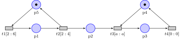
Assuming the obvious naming function mapping to "A", and so on, the net in Fig. 1(b) is represented as the following term of sort Net:
We define some useful operations on markings, such as _+_ and _-_:
(This definition assumes that each place in appears once in and +.) The function _-_ on markings is defined similarly. The following functions compare markings and check whether a transition is active in a marking:
Dynamics.
We define the dynamics of ITPNs as a Maude “interpreter” for such nets. The concrete ITPN semantics in [3] dynamically adjusts the “time intervals” of non-inhibited transitions when time elapses. Unfortunately, the definitions in [3] seem slightly contradictory (even with non-empty firing intervals): On the one hand, time interval end-points should be non-negative, and only enabled transitions have intervals in the states; on the other hand, the definition of time and discrete transitions in [3] mentions and , which seems superfluous if all end-points are non-negative. Taking the definition of time and transition steps in [3] (our Definition 2.3) leads us to time intervals where the right end-points of disabled transitions could have negative values. This has some disadvantages: (i) “time values” can be negative numbers; (ii) we have counterintuitive “intervals” where the right end-point is smaller than the left end-point; (iii) the reachable “state spaces” (in suitable discretizations) could be infinite when these negative values could be unbounded.
To have a simple and well-defined semantics, we use “clocks” instead of “decreasing intervals”; a clock denotes how long the corresponding transition has been enabled (but not inhibited). Furthermore, to reduce the state space, the clocks of disabled transitions are always zero. The resulting semantics is equivalent to the (most natural interpretation of the) one in [3] in a way made precise in Theorem 3.5.
The sort ClockValues denotes sets of ;-separated terms -> , where is the (label of the) transition and represents the current value of ’s “clock.”
The states in are terms : : of sort State, where represents the current marking, the current values of the transition clocks, and the representation of the Petri net:
The following rewrite rule models the application of a transition L in the net (L : PRE ---> POST inhibit INHIBIT in INTERVAL) ; NET. Since _;_ is declared to be associative and commutative, any transition L in the net can be applied using this rewrite rule:
The transition L is active (enabled and not inhibited) in the marking M and its clock value T is in the INTERVAL. After performing the transition, the marking is (M - PRE) + POST, the clock of L is reset333Since in our semantics clocks of disabled transitions should be zero, we can safely set the clock of L to 0 in this rule. and the other clocks are updated using the following function:
The second rewrite rule in specifies how time advances. Time can advance by any value T, as long as time does not advance beyond the time when an active transition must be taken. The clocks are updated according to the elapsed time T, except for those transitions that are disabled or inhibited:
This rule is not executable ([nonexec]), since the variable T, which denotes how much time advances, only occurs in the right-hand side of the rule. T is therefore not assigned any value by the substitution matching the rule with the state being rewritten. This time advance T must be less or equal to the smallest remaining time until the upper bound of an active transition in the marking M is reached:444To increase readability, we sometimes replace parts of Maude code or output from Maude analyses by ‘...’.
The function increaseClocks increases the transition clocks of the active transitions by the elapsed time:
The following function formalizes how markings and nets are represented as terms, of respective sorts Marking and Net, in rewriting logic.555 is parametrized by the naming function ; however, we do not show this parameter explicitly.
Definition 3.2
Let be an ITPN. Then is defined by
, where we can omit entries . The Maude representation of the net is
the term
of sort Net, where, for each , is
: -->
inhibit
in [ : ].
3.2 Correctness of the semantics
In this section we show that our rewriting logic semantics correctly simulates any ITPN . More concretely, we provide a bisimulation result relating behaviors from in with behaviors in starting from the initial state : initClocks() : , where initClocks() is the clock valuation that assigns the value 0 to each transition (clock) for each transition (label) in .
Since a transition in consists of a delay followed by a discrete transition, we define a corresponding rewrite relation combining the tick and applyTransition rules, and prove the bisimulation for this relation.
Definition 3.3
Let be terms of sort State in . We write if there exists a such that is a one-step rewrite applying the tick rule in and is a one-step rewrite applying the applyTransition rule in . Furthermore, we write to indicate that there exists a sequence of rewrites from to .
The following relation relates our clock-based states with the changing-interval-based states; the correspondence is a straightforward function, except for the case when the upper bound of a transition is :
Definition 3.4
Let be an ITPN and be its concrete semantics. Let denote the set of -equivalence classes of ground terms of sort State in . We define a relation , relating states in the concrete semantics of to states (of sort State) in , where for all states , if and only if and and for each transition ,
-
•
the value of in is 0 if in not enabled in ;
-
•
otherwise:
-
–
if then the value of clock in is ;
-
–
otherwise, if then has the value in ; otherwise, the value of in could be any value .
-
–
Theorem 3.5
Let be an ITPN,
and . Then,
is a bisimulation between the transition systems
and
.
Proof 3.6
By definition , since all clocks are 0 in , so that these clocks satisfy all the constraints in Definition 3.4 since in the initial state. Hence, condition (i) for being a bisimulation is satisfied. Condition (ii) follows from the two lemmas below.
Lemma 3.7
If and then there is a such that and .
Proof 3.8
Since , we have that there exists an intermediate pair such that and .
For the first step (), since , there exists a such that , either or and . In both cases we have that . Now, letting T , it must be the case that T <= mte(, , ). This is because mte(, , ) is defined to be equal to the minimum difference between and the clock value of out of all . That is, it is the maximum time that can elapse before an enabled transition reaches the right endpoint of its interval. In other words, an upper limit for . Hence, the tick-rule can be applied to with all enabled clocks having their time advanced by .
For the second step (), since , the transition is active and . Since , the clock of transition must be in the interval by definition of for . This is precisely the condition for applying the applyTransition-rule to the resulting state of the previous tick-rule application.
Lemma 3.9
If
and
,
then there exists a state
such that and
.
Proof 3.10
Since ,
we have that there exists an intermediate state
such that and
.
For the first step , since , there is a T <= mte(, , ). Now, as in the previous lemma, since the mte is an upper limit for , we have that there exists a time transition with equal to the T used in the above tick-rule application so that .
For the second step , since , there must be a transition which is active and whose clock is in the interval . By definition of on , This is precisely the condition for the discrete step to . Hence, and .
3.3 Some variations of
This section introduces the theories and as two variations of . avoids consecutive applications of the tick rule. This is useful for symbolic analysis, since in concrete executions of , a tick rule application may not advance time far enough for a transition to become enabled. adds a “global clock”, denoting how much time has elapsed in the system. This allows for analyzing time-bounded properties (can a certain state be reached in a certain time interval?).
3.3.1 The theory
To avoid consecutive tick
rule applications, we add a new component—whose value is
either tickOk or tickNotOk—to the global
state. The tick rule can only be applied when this new component of the
global state has the value tickOk. We therefore add a new
constructor _:_:_:_ for these extended global states, a new
sort TickState with values tickOk and
tickNotOk, and modify (or add) the two rewrite rules below:
Theorem 3.11
Let be a ground term of sort State in . Then
if and only if
Proof 3.12
For the () side, it suffices to follow in the same execution strategy as in . For (), it suffices to perform the following (reachability-preserving) change in the trace: the application of two consecutive tick rules with and are replaced by a single application of tick with . This is enough to show that the same trace can be obtained in .
Although reachability is preserved, an “arbitrary” application of the tick rule in , where time does not advance far enough for a transition to be taken, could lead to a deadlock in which does not correspond to a deadlock in .
3.3.2 The theory
To analyze whether a certain state can be reached in a certain time interval, and to enable time-bounded analysis where behaviors beyond the time bound are not explored, we add a new component, denoting the “global time,” to the global state:
The tick and applyTransition rules are modified as expected. For instance, the rule tick becomes:
For analyses up to some time bound , we add a conjunct GT + T <= to the condition of this rule to stop executing beyond the time bound.
Let and be terms of sort State in . We say that is reached in time from , written , if and is the sum of the values taken by the variable T in the different applications of the rule tick in such a trace.
Theorem 3.13
if and only if
Proof 3.14
From Theorem 3.11, we know that the tickOk/tickNotOk strategy can be followed in to produce an equivalent trace. Using that trace, the result follows trivially by noticing that applications of tick in with T () match applications of tick in with the same instance of T, thus advancing the global clock in exactly time units.
4 Explicit-state analysis of ITPNs in Maude
The theories – cannot be directly executed in Maude, since the tick rule introduces a new variable T in its right-hand side. Following the Real-Time Maude [14, 32] methodology for analyzing dense-time systems, although we cannot cover all time points, we can choose to “sample” system execution at some time points. For example, in this section we change the tick rule to increase time by one time unit in each application:
Analysis with such time sampling is in general not sound and complete, since it does not cover all possible system behaviors: for example, if some transition’s firing interval is , we could not execute that transition with this time sampling. Nevertheless, if all interval bounds are natural numbers, then “all behaviors” should be covered.
We can therefore quickly prototype our specification and experiment with different parameter values, before applying the sound and complete symbolic analysis and parameter synthesis methods developed in the following sections.
The term net3(,) represents an instance of a more general version of the net in Fig. 2, where the interval for transition is , and where the parameters and are instantiated with values and :
The initial marking in Fig. 2 is represented by the term init3:
We can simulate 2000 steps of the net with different parameter values:
To further analyze the system, we define a function k-safe, where k-safe(,) holds iff the marking does not have any place with more than tokens:
We can then quickly (in 5ms) check whether the net is 1-safe when transition has interval by searching for a reachable state whose marking M has some place holding more than one token (not k-safe(1,M)):
The net is not 1-safe: we reached a state with two tokens in place . However, the net is 1-safe if ’s interval is instead :
Further analysis shows that net3(3,4) is 2-safe, but that net3(3,5) is not even 1000-safe.
We can also analyze concrete instances of our net by full linear temporal logic (LTL) model checking in Maude. For example, we can define a parametric atomic proposition “placehastokens”, which holds in a state iff its marking has exactly tokens in place :
Then we can check properties such as whether in each behavior of the system, there will be infinitely many states where has no tokens and infinitely many states where it holds one token:666[], <>, /\, and ~ are the Maude representations of corresponding (temporal) logic operators (“always”), (“eventually”), conjunction, and negation.
We know that net3(3,4) can reach markings with two tokens in ; but is this inevitable (i.e., does it happen in all behaviors)?
The result is a counterexample showing a path where never holds two tokens.
We also obtain a “time sampling” specification for time-bounded analyses following the techniques for ; namely, by adding a global time component to the state:
and modifying the tick rule to increase this global clock according to the elapsed time. Furthermore, for time-bounded analysis we add a constraint ensuring that system execution does not go beyond the time bound :
By setting to 1000, we can simulate one behavior of the system net3(3,5) up to time 1000:
We can then check whether net3(3,4) is one-safe in the time interval by setting in the tick rule to 10, and execute following command:
This shows that the non-one-safe marking can be reached in eight time units. It is worth noticing that this result only shows that (one of) the shortest rewrite path(s) to a non-one-safe marking has duration 8. We cannot conclude from this, however, that such a state cannot be reached in shorter time, which could be possible with more rewrite steps.
5 Parameters and symbolic executions
Standard explicit-state Maude analysis of the theories – cannot be used to analyze all possible behaviors of PITPNs for two reasons:
-
1.
The rule tick introduces a new variable T in its right-hand side, reflecting the fact that time can advance by any value T <= mte(...); and
-
2.
analyzing parametric nets with uninitialized parameters is impossible with explicit-state Maude analysis of concrete states. Note, for instance, that the condition T in INTERVAL in rule applyTransition will never evaluate to true if INTERVAL is not a concrete interval, and hence the rule will never be applied.
Maude-with-SMT analysis of symbolic states with SMT variables can solve both issues, by symbolically representing the time advances T and the net’s uninitialized parameters. This enables analysis and parameter synthesis methods for analyzing all possible behaviors in dense-time systems with unknown parameters.
This section defines a rewrite theory that faithfully models PITPNs and that can be symbolically executed using Maude-with-SMT. We prove that (concrete) executions in are captured by (symbolic) executions in , and vice versa. We also show that standard folding techniques [42] in rewriting modulo SMT are not sufficient for collapsing equivalent symbolic states in . We therefore propose a new folding technique that guarantees termination of reachability analyses in when the state-class graph of the encoded PITPN is finite. We present two implementations of the folding procedure that we benchmark in Section 6.
5.1 The symbolic rewriting logic semantics
We define the “symbolic” semantics of PITPNs using the rewrite theory , which is the symbolic counterpart of , instead of basing it on , since a symbolic “tick” step represents all possible tick steps from a symbolic state. We therefore do not introduce deadlocks not possible in the corresponding PITPN by disallowing multiple consecutive (symbolic) applications of the tick rule.
is obtained from by replacing the sort Nat in markings and the sort PosRat for clock values with the corresponding SMT sorts IntExpr and RExpr. (The former is only needed to enable reasoning with symbolic initial states where the number of tokens in a location is unknown). Moreover, conditions in rules (e.g., M1 <= M2) are replaced with the corresponding SMT expressions of sort BoolExpr. The symbolic execution of using Maude with SMT will accumulate and check the satisfiability of the constraints needed for a parametric transition to happen.
We declare the sort Time as follows:
where RExpr is the sort for SMT reals. (We add constraints to the rewrite rules to guarantee that only non-negative real numbers are considered as time values.) Besides rational constants of sort Rat, terms in RExpr can be also SMT variables.
Intervals are defined as in : op ‘[_:_‘] : Time TimeInf -> Interval. Since RExpr is a subsort of Time, an interval in may contain SMT variables. This means that a parametric interval in a PITPN can be represented as the term [a : b], where a and b are variables of sort RExpr.
The definition of markings, nets, and clock values is similar to the one in Section 3.1. We only need to modify the following definition for markings:
Hence, in a pair |-> , is an SMT integer expression that could be/include SMT variable(s).
Operations on markings and intervals remain the same, albeit with the appropriate SMT sorts. Since the operators in Maude for Nat and Rat have the same signature than those for IntExpr and RExpr, the specification needs few modifications. For instance, the new definition of M1 <= M2 is:
where <= in N1 <= N2 is a function op _<=_ : IntExpr IntExpr -> BoolExpr.
Symbolic states in are defined as follows:
The rewrite rules in act on symbolic states that may contain SMT variables. Although these rules are similar to those in , their symbolic execution is completely different. Recall from Section 2 the theory transformation to implement symbolic rewriting in Maude-with-SMT. In the resulting theory , when a rule is applied, the variables occurring in the right-hand side but not in the left-hand side are replaced by fresh variables, represented as terms of the form rr(id) of sort RVar (with subsort RVar < RExpr) where id is a term of sort SMTVarId (theory VAR-ID in Maude-SE). Moreover, rules in act on constrained terms of the form , where in this case is a term of sort State and is a satisfiable SMT boolean expression (sort BoolExpr). The constraint is obtained by accumulating the conditions in rules, thereby restricting the possible values of the variables in .
The tick rewrite rule in is
The variable T is restricted to be a non-negative real number and to satisfy the following predicate mte, which gathers the constraints to ensure that time cannot advance beyond the point in time when an enabled transition must fire:
This means that, for every transition L, if the upper bound of the interval in L is inf, no restriction on T is added. Otherwise, if L is active at marking M, the SMT ternary operator ?: (checking to choose either or ) further constrains T to be less than T2 - R1. The definition of increaseClocks also uses this SMT operator to represent the new values of the clocks:
The rule for applying a transition is defined as follows:
When applied, this rule adds new constraints asserting that the transition L can be fired (predicates active and _in_) and updates the state of the clocks:
In the example below, k-safe(,) is a predicate stating that the marking does not have more than tokens in any place.
Example 5.1
Let and be the Maude terms representing, respectively, the PITPN and the initial marking shown in Fig. 2. The term below includes an SMT variable representing the parameter in transition :
The Maude’s commands introduced in LABEL:sec:analysis allow us to answer the question whether it is possible to reach a state with a marking with more than one token in some place. As shown in Example 5.9, Maude positively answers this question and the resulting accumulated constraint tells us that such a state is reachable (with 2 tokens in ) if rr("a") >= 4.
Terms of sort Marking in may contain expressions with parameters (i.e., variables) of sort IntExpr. Let denote the set of such parameters and a valuation function for them. We use to denote a mapping from places to IntExpr expressions including parameter variables. Similarly, denotes a mapping from transitions to RExpr expressions (including variables). We write to denote the ground term where the parameters in markings are replaced by the corresponding values . Similarly for , we use to denote the above rewriting logic representation of nets in .
Let be the constrained term of sort State in and assume that . By construction, if for all all markings (sort IntExpr), clocks and parameters (sort RExpr) are non-negative numbers, then this is also the case for all .
The following theorem states that the symbolic semantics matches all the behaviors resulting from a concrete execution of with arbitrary parameter valuations and . Furthermore, for all symbolic executions with parameters, there exists a corresponding concrete execution where the parameters are instantiated with values consistent with the resulting accumulated constraint.
Theorem 5.2 (Soundness and completeness)
Let be a PITPN and be a marking possibly including parameters.
(1) Let be the constraint . If
then, there exist a parameter valuations and a parameter marking valuation s.t.
where the constraint is satisfiable, and .
(2) Let be a parameter valuation and a parameter marking valuation. Let be the constraint . If
then
where , and .
Proof 5.3
The symbolic counterpart of the theory , that adds a component to the state denoting the “global time”, can be defined similarly. We have also defined a third symbolic theory that replaces the applyTransition rule in with the following one:
Hence, in , two consecutive applications of applyTransition (without applying tick in between) are not allowed.
5.2 A sound and complete folding method for symbolic reachability
Reachability analysis should terminate for both positive and negative queries for nets with finite parametric state-class graphs. However, the state space resulting from the (symbolic) execution of the theory is infinite even for such nets, and it will not terminate when the desired states are unreachable. We note that the standard search commands in Maude stop exploring from a symbolic state only if it has already visited the same state. Due to the fresh variables created in whenever the tick rule is applied, symbolic states representing the same set of concrete states are not the same, even though they are logically equivalent, as exemplified below.
Example 5.4
Let be the constraint . The following command, trying to show that the PITPN in Fig. 2 is 1-safe if the parameter satisfies , does not terminate.
Furthermore, the command
searching for reachable states where will produce infinitely many (equivalent) solutions, including, e.g., the following constraints:
⬇ Solution 1: #p5-9:IntExpr === 1 and #t3-9:RExpr + a:RExpr - #t2-9:RExpr <= 0/1 and ... Solution 2: #p5-16:IntExpr === 1 and #t3-16:RExpr + a:RExpr - #t2-16:RExpr <= 0/1 and ...
where the variables created by the search procedure start with #
and end with a number taken from a sequence to guarantee freshness.
Let and be, respectively, the
constrained terms found in Solution 1 and Solution 2.
In this particular output, is obtained by further rewriting
.
The variables representing the state of markings and clocks
(e.g., #p5-9 in and #p5-16 in ) are clearly different,
although they
represent the same set of concrete values ().
Since constrains are accumulated when a rule is applied, we note that
equals for some , and
.
The usual approach for collapsing equivalent symbolic states in rewriting modulo SMT is subsumption [42]. Essentially, we stop searching from a symbolic state if, during the search, we have already encountered another (“more general”) symbolic state that subsumes (“contains”) it. More precisely, let and be constrained terms. Then if there is a substitution such that and the implication holds. In that case, . A search will not further explore a constrained term if another constrained term with has already been encountered. It is known that such reachability analysis with folding is sound (does not generate spurious counterexamples [44]) but not necessarily complete (since does not imply ).
Example 5.5
Let and be the resulting constraints in the two solutions found by the second search command in Example 5.4. Let be the substitution that maps #p-9 to #p-16 and #t-9 to #t-16 for each place and transition . The SMT solver determines that the formula is satisfiable (and therefore is not valid). Hence, a procedure based on checking this implication will fail to determine that the state in the second solution can be subsumed by the state found in the first solution.
The satisfiability witnesses of can give us some ideas on how to make the subsumption procedure more precise. Assume that carries the information for some clock represented by and is a tick variable subject to . Assume also that in , the value of the same clock is subject to . Let . Note that does not imply (take, e.g., the valuation and ). The key observation is that, even if and are both constrained to be in the interval (and hence represent the same state for this clock), the assignment of in the antecedent does not need to coincide with the one for in the consequent of the implication.
In the following, we propose a subsumption relation that solves the aforementioned problems. Let be a constrained term where is a term of sort State. Consider the abstraction of built-ins for , where is as but it replaces the expression in markings () and clocks () with new fresh variables. The substitution is defined accordingly. Let . We use to denote the constrained term . Intuitively, replaces the clock values and markings with fresh variables and the boolean expression constrains those variables to take the values of clocks and marking in . From [38] we can show that .
Note that the only variables occurring in are those for parameters (if any) and the fresh variables in (representing the symbolic state of clocks and markings). For a constrained term , we use to denote the formula where .
Definition 5.6 (Relation )
Let and be constrained terms where and are terms of sort State. Moreover, let and , where . We define the relation on constrained terms so that whenever there exists a substitution such that and the formula is valid.
The formula hides the information about all the tick variables as well as the information about the clocks and markings in previous time instants. What we obtain is the information about the parameters and the values of the clocks and markings “now”. Moreover, if and above are both tickOk states (or both tickNotOk states), and they represent two symbolic states of the same PITPN, then and always match ( being the identity on the variables representing parameters and mapping the corresponding variables created in and ).
Theorem 5.7 (Soundness and completeness)
Let and be constrained terms in representing two symbolic states of the same PITPN. Then, iff .
Proof 5.8
Let and , where . Let and . By construction, , , and . It suffices to show iff .
() Assume . Then, and are -unifiable (witnessed by ). Since has no duplicate variables and only contains structural axioms for , by the matching lemma [38, Lemma 5], there exists a substitution with (equality modulo ACU). Since any built-in subterm of is a variable in , is a renaming substitution and thus .
Suppose is not valid, i.e., is satisfiable. Let be the set of free variables in . Notice that . Let be a ground substitution that represents a satisfying valuation of . Then, but , which is a contradiction.
() Assume . There exists a substitution such that and is valid. Let be the set of free variables in . As mentioned above, and . Let . Then, for some ground substitution , and holds. From the assignments in , we can build a valuation making true and, by assumption, making also true . Hence, there exists a ground substitution (that agrees on the values assigned in ) such that holds and . Notice that . Therefore, .
5.2.1 Two versions of symbolic reachability analysis based on the folding procedure
The implementation of the folding procedure in Maude requires the specification of the subsumption relation that, in turns, requires dealing with the existentially quantified variables in . At the time of publishing the conference version of this paper [35], the only method available for checking the satisfiability of existentially quantified formulas in Maude involved the call to the existential quantifier elimination procedure of the SMT solver Z3. Recently [34], we have implemented the well-known Fourier-Motzkin elimination (FME) procedure [45] using equations in Maude, and it is independent of the SMT solver connected to Maude. (As demonstrated in Section 6, this change has an important effect on the performance of the analysis).
Building on this FME equational theory, we propose two different implementations/versions of symbolic reachability analysis based on the folding procedure:
-
1.
The first one is based on a simple theory transformation that adds to the (symbolic) state the already visited (symbolic) states in that execution branch, and prevents a rule to be applied if the resulting state would be subsumed by the states already seen in this branch. This new theory can be used directly with the standard search command in Maude. However, this procedure cannot fold equivalent states appearing in different branches of the search tree.
-
2.
The second implementation/version solves this problem by defining, using Maude’s meta-level facilities, a breath-first search procedure that keeps a global set of already visited states in all the branches across the search tree.
The first implementation (theory ).
A term in the theory defined below also stores the states that have been visited before reaching . Additionally, a rewrite step from to a term is only possible if the state represented by is not subsumed by the already visited states. Hence, theory can be used to perform reachability analysis with folding as illustrated in Example 5.9.
We transform the theory into a rewrite theory that rewrites terms of the form . The term , of sort Map (defined in Maude’s prelude [13]), is a set of entries of the form where is a Marking and is a BoolExpr expression. stores the already visited states, and is the accumulated constraint leading to the state where the marking is . The theory defines the operator subsumed that checks whether the symbolic state in the first parameter is subsumed by one of the states stored in .
A rule in is transformed into the following rule in :
where is a BoolExpr variable and is an abstraction of built-ins for and . Note that the transition happens only if the new state is not subsumed by an already visited state. The function checks whether there is an entry where is the marking in the term . If this is the case, this entry is updated to . Otherwise, a new entry is added to the map. In the first case, a symbolic state where the marking is was already visited, but with constraints for the clocks and parameters that are not implied by (and hence not subsumed). Therefore, the new state is merged, and the marking can be reached by satisfying either or .
In , for an initial constraint on the parameters,
the command
search [,] empty : =>* : such that smtCheck(
answers the question whether it is possible to reach a symbolic state that matches and satisfies the condition . In the following, we denote by the following term (of sort State): .
Example 5.9
Consider the PITPN in Fig. 2. Let be the marking in the figure and be the constraint . The command
These operators allow us to:
-
•
perform reachability analysis and solve parameter synthesis problems using the theories (search-sym) and (search-sym2, where applications of rules tick and applyTransition must be interleaved);
-
•
perform reachability analysis with folding using the theory and the new breath-first search procedure with a global set of already visited states (folding);
-
•
perform time-bounded reachability analysis (search in-time) using the theory (that adds to the state the global clock);
-
•
solve safety synthesis problems (AG-synthesis);
-
•
analyze a net with a user-defined strategy (strat-rew); and
-
•
model check non-nested (T)CTL formulas (A-model-check and E-model-check).
The parameters of these commands are explained next.
The parameters of sort Nat are both optional and can be omitted in the reachability analysis commands. They can be used to limit the number of solutions to be returned and the maximal depth of the search tree. The parameter of sort Qid (quoted identifiers, as ’MODEL) is the name of the module with the user-defined PITPN. The initial state (sort InitState) is a triple containing the definition of the net, the initial marking and the initial constraint on the parameters:
We define the following atomic propositions, or state predicates; these will be used to define the (un)desired properties of our (symbolic) states:
The atomic formula p n () states that the current marking satisfies where, for instance, holds in a state if place holds less than tokens. Similarly, t r is true in a state where the value of the clock associated to transition satisfies . The predicate reach() is true in a marking if , and k-bounded() is true in a state where each place holds less than or equal to tokens. For temporal properties (see Section 5.5 for more details), the formula in-time is true if the current value of the global clock is in . Other predicates can be built with the usual boolean operators.
The following operators and equations (we present only some cases) define when a state satisfies a state property , denoted by :
Since the state may contain SMT variables, a call to the SMT solver is needed to determine whether the state entails the given property. The functions constraint and marking are the expected projection functions, returning the appropriate components of the state.
Terms of sort LResult are lists of terms of the following sort Result:
where the term when represents the fact that the marking can be reached with accumulated constraint .
In the operator/command strat-new, it is possible to limit only the number of solutions to be returned, when analyzing a system under a given user-defined Strategy. As explained below, (T)CTL and (T)LTL temporal Formulas can be model checked with a time bound specified by the last parameter in the operators A-model-check and E-model-check.
The definition of the above search, folding, synthesis, and model-checking operators use the META-LEVEL module in Maude (for meta-programming) to:
-
•
define a new theory (a term of sort Module, a meta-representation of a rewrite theory) that imports both the needed rewrite theory (e.g., ) and the module with the user-defined net;
-
•
compute the meta-representation of the initial state according to the theory to be used;
-
•
invoke the needed Maude command (e.g., metaSearch) to search for a solution; and
-
•
simplify the resulting constraints by invoking the FME procedure, eliminating all the SMT variables except those representing parameters. As shown below, this last step allows for finding the constraints on the parameter values that enable certain execution paths.
In the following subsections we exemplify the use of these operators and how they can be used to solve interesting problems of PITPNs.
5.3 Parameter synthesis
EF-synthesis is the problem of computing parameter values such that there exists a run of that reaches a state satisfying a given state predicate . The safety synthesis problem AG is the problem of computing the parameter values for which states satisfying are unreachable.
Search (with or without folding) provides a semi-decision procedure for solving EF-synthesis problems (which is undecidable in general). The synthesis problem AG is solved by finding all the solutions for EF (therefore a search procedure with folding is necessary to guarantee termination when possible) and then negating the disjunction of all these solutions/constraints. If the resulting constraint is unsatisfiable, it means that there are no values for the parameters guaranteeing that non--states are unreachable and hence, there is no solution for . In that case, our procedure returns the constraint false (see Example 5.13).
Example 5.10
Example 5.1 shows an EF-synthesis problem: find values for the parameter such that a state with at least two tokens in some place can be reached. If , the command
finds a state where the place has two tokens. The resulting constraint (after eliminating all the SMT variables but not those of the parameters) determines that this is possible when . The same solution can be found with the commands search-sym2, search-folding, and folding.
With the same model, we can synthesize the values for the parameter to reach a state where the difference between the values of the clocks in transitions and is bigger than, for instance, :
Roméo only supports properties over markings. The state predicate in the previous example includes also conditions on the values of the “clocks” associated to the transitions, where each clock denotes how long the corresponding transition has been active without being fired.
To solve the safety synthesis problem AG, the AG-synthesis procedure iteratively calls the command folding to find a state reachable from the initial marking , with initial constraint , where does not hold. If such state is found, with accumulated constraint , the folding command is invoked again with initial constraint . This process stops when no more reachable states where does not hold are found, thus solving the AG synthesis problem.
Example 5.11
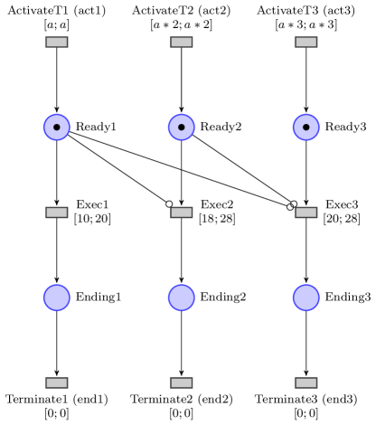
Consider the PITPN in Fig. 3, taken from [46], with a parameter and three parametric transitions with respective firing intervals , and . Roméo can synthesize the values of the parameter making the net 1-safe, subject to initial constraint . The same query can be answered in Maude:
The first counterexample found assumes that . If , folding does not find any state not satisfying k-bounded(1). This is the same answer found by Roméo.
Our symbolic theories can have parameters (variables of sort IntExpr) in the initial marking. This opens up the possibility of using Maude-with-SMT to solve synthesis problems involving parametric initial markings. For instance, we can determine the initial markings that make the net -safe.
Example 5.12
Consider the net in Fig. 2, the initial constraint stating that and the initial marking as in the figure. The following command shows that the net is 1-safe if :
Assume that we fix the parameter to be, for instance, . We may ask whether the net continues to be 1-safe when the number of tokens in places and is unknown. For that, consider the parametric initial marking with parameters and denoting the number of tokens in places and , respectively, and the initial constraint stating that , , and . The execution of the following command:
determines that the net is 1-safe only when both places and are initially empty.
Example 5.13
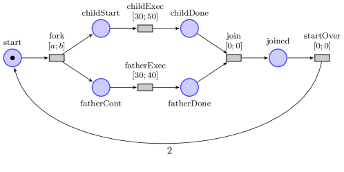
Consider the PITPN tutorial in Fig. 4, taken from the Roméo website. This model has been modified so that transition startOver produces two tokens, thus leading to a non-1-safe system. The first solution to EF is the initial constraint already present in this net’s (i.e., no further constraints on these parameters are needed to reach the non-1-safe state). Hence, there is no solution for the corresponding AG-synthesis problem:
5.4 Analysis with user-defined strategies
Maude’s strategy language [47] allows users to define execution strategies for their rewrite theories. This section explains how we can analyze all possible behaviors of a PITPN allowed by a user-defined strategy for the net. Such analysis is supported by our framework through the command
This command rewrites, using the meta-level function metaSrewrite, the term following the strategy ; match S s.t. check(S, ) and the rules in (to guarantee termination when possible), and outputs the first solutions. The strategy match s.t. check(S, ) fails whenever the state does not satisfy the state property . Hence, this command returns the first reachable states following the strategy that satisfy .
Example 5.14
We analyze net in Fig. 2 when all its executions (must) adhere to the following strategy t3-first: whenever transition and some other transition are enabled at the same time, then fires first. This execution strategy can be specified as follows using Maude’s strategy language:
Starting with the initial constraint , the execution of the command
shows that there are 12 possible reachable symbolic states when this strategy is applied. Furthermore, the execution of the command
returns no such non-1-safe symbolic states (the empty list nil). This shows that all markings reachable with the strategy t3-first are 1-safe. Note that this is not the case when the system behaviors are not restricted by any strategy. As shown in Example 5.12, the parameter needs to be further constrained () to guarantee 1-safety.
5.5 Analyzing temporal properties
This section shows how Maude-with-SMT can be used to analyze the temporal properties supported by Roméo [7], albeit in a few cases without parametric bounds in the temporal formulas. Roméo can analyze the following temporal properties:
where is the existential/universal path quantifier, and are state predicates on markings, and is a time interval , where and/or can be parameters and can be . For example, says that in each path from the initial state, a marking satisfying is reachable in some time in . The bounded response denotes the formula (each -marking must be followed by a -marking within time ).
Since queries include time bounds, we use the theory (that adds a component representing the global clock) so that the term represents a state of the system where the “global clock” is .
Some of the temporal formulas supported by Roméo can be easily verified using reachability commands similar to the ones presented in the previous section. The property can be verified using the command
where states that all parameters are non-negative numbers (and adds the net’s constraints, including that firing intervals are not empty), and and can be variables representing parameters to be synthesized.
The dual property can be checked by analyzing .
Example 5.15
Consider the PITPN in Example 5.11 with (interval) parameter constraint . The property can be verified with the following command, which shows that the desired property holds when the upper time bound in the timed temporal logic formula satisfies .
The bounded response formula can be verified using a simple theory transformation on followed by reachability analysis. The theory transformation adds a new constructor for the sort State to build terms of the form , where is either noClock or clock(); the latter represents the time () since a -state was visited, without having been followed by a -state. The rewrite rules are adjusted to update this new component as follows. The new tick rule updates clock(T1) to clock(T1 + T) and leaves noClock unchanged. The rule applyTransition is split into two rules:
In the first rule, if a -state is encountered, the new “-clock” is reset to noClock. In the second rule, this “-clock” starts running if the new state satisfies but not . The query can be answered by searching for a state where a -state has not been followed by a -state before the deadline :
Reachability analysis cannot be used to analyze the other properties supported by Roméo (, and and its dual ). While developing a full SMT-based timed temporal logic model checker is future work, we can combine Maude’s explicit-state model checker and SMT solving to solve these (and many other) queries. On the positive side, and beyond Roméo, we can use full LTL.
The timed temporal operators , , and , written <>, U, and [], respectively, in our framework, can be defined on top of the (untimed) LTL temporal operators in Maude (<>, [], and U) as follows :
For this fragment of non-nested timed temporal logic formulas, it is possible to model check universal and existential quantified formulas with the following commands:
Non-nested -formulas can be directly model checked by calling Maude’s LTL model checker:
modelCheck(STATE, F) == true. For the -formulas, what we need is to check whether does not hold: modelCheck(STATE , ~ F) =/= true. The “in time ” part in the command is optional, and it is used to perform bounded model checking, forbidding the application of the tick rule when the global clock is beyond . This parameter is specially important for -formulas that require exploring the whole state space to check whether does not hold.
Example 5.16
Consider the PITPN tutorial in Fig. 4. Below we model check some formulas and, in comments, we explain the results:
6 Benchmarking
We have used three PITPNs to compare the performance of our Maude-with-SMT analysis with that of Roméo (version 3.9.4), and with that of our previous implementation presented in [35]. We compare the time it takes to solve the synthesis problem EF() (i.e., place holds more than tokens), for different places and , and to check whether the net is -safe.
The PITPNs used in our experiments are: the producer-consumer system [43] in Fig. 2, the scheduling system [46] in Fig. 3, and the tutorial system in Fig. 4 taken from the Roméo website and modified as explained in Example 5.16. For EF-synthesis problems, we benchmark the performance of commands implementing reachability with and without folding: search-sym (EF-synthesis using theory , which does not use folding), search-sym2 (theory , interleaving tick and applyTransition rules), search-folding (EF-synthesis with folding using the theory , which uses Maude’s search command and folds symbolic states in the same branch of the search tree) and folding (our own meta-level implementation of breath-first search that folds symbolic states across all branches in the search tree). For safety synthesis problems, we use the command AG-synthesis.
We ran all the experiments on a Dell Precision Tower 3430 with a processor Intel Xeon E-2136 6-cores @ 3.3GHz, 64 GiB memory, and Debian 12. Each experiment was executed using Maude in combination with three different SMT solvers: Yices2 (Maude 3.3.1), CVC4 (Maude-SE 3.0 [31]) and Z3 (Maude-SE 3.0). We use a timeout of 5 minutes. The reader can find the data of all the experiments and the scripts needed to reproduce them in [36].
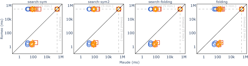
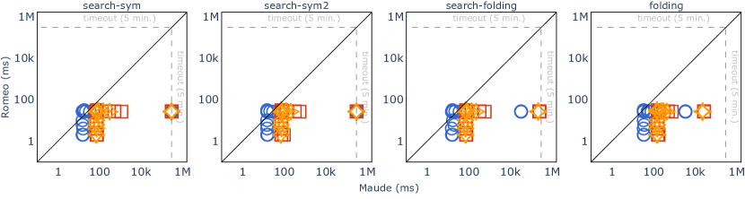
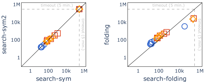
Figure 5 shows the execution times of Roméo and Maude in log-scale for the three benchmarks. The diagonal line represents when the two systems would get the same result to analyze the property EF() (Figs. 5(a), 5(b) and 5(c)) and 1-safety (Fig. 5(d)). An item (or “point”) above the diagonal line represents a problem instance where Maude outperforms Roméo. Items in the horizontal line at the top of each figure represent instances where Roméo timed out and Maude was able to complete the analysis. Items on the vertical line on the right represent instances where Maude timed out and Roméo completed the analysis.
Executing Maude with Yices2 clearly outperforms executing Maude together with the other two SMT solvers. For the EF-synthesis problems in Fig. 5, it is worth noticing that: all the queries but not (where Roméo also times out) could be solved in the producer-consumer benchmark; the reduction of the state space achieved by the folding procedures (commands search-folding and folding) were needed to solve the query in scheduler; and all the queries in tutorial were solved by all the commands using Yices2 and CVC4. All the AG-synthesis problems could be solved by the command AG-synthesis (that uses the implementation of folding at the meta-level).
In some reachability queries, Maude outperforms Roméo. More interestingly, our approach terminates in cases where Roméo does not (items in the horizontal line at the top of Fig. 5(a) and Fig. 5(c)). Our results are proven valid when injecting them into the model and running Roméo with these additional constraints. This phenomenon happens when the search order leads Roméo in the exploration of an infinite branch with an unbounded marking.
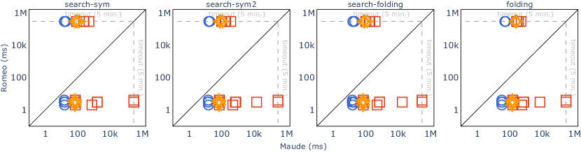
In Fig. 6 we compare the performance of the different Maude commands for EF-synthesis and AG-synthesis. For some instances, search-sym2 is marginally faster than the command search-sym. In general, the command search-folding is faster than the command folding. However, the extra reduction of the search space (folding states in different branches of the search tree) allows folding to solve some instances faster in the scheduling benchmark (see the three items on the right in Fig. 6(b)).
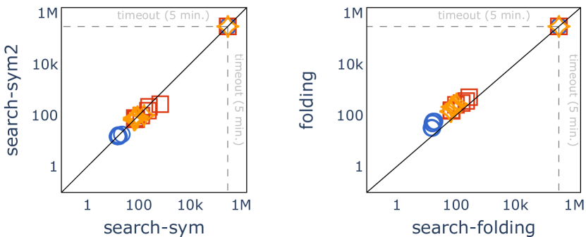
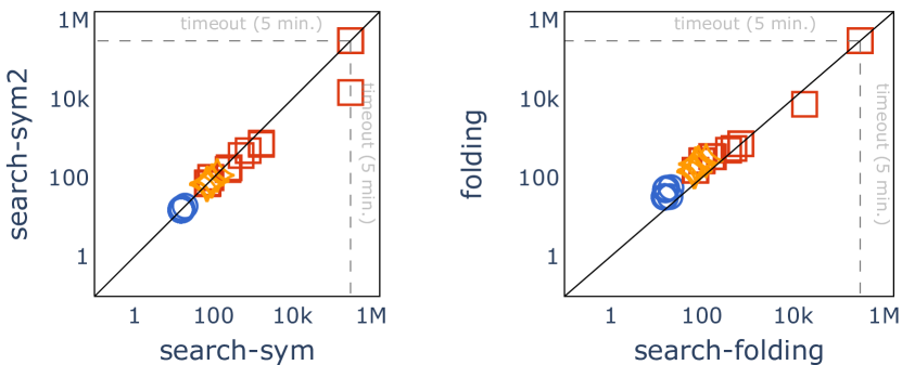
We have also compared the performance of the folding analysis presented in the conference version of this paper [35] and the current one. As explained in Section 5.2.1, the current implementation uses the FME procedure implemented as an equational theory in Maude, while the previous one relies on the procedure implemented in Z3. The results are given in Fig. 7 and they clearly indicate that the new implementation is more efficient than the previous one.

7 Related work
Tool support for parametric time Petri nets.
We are not aware of any tool for analyzing parametric time(d) Petri nets other than Roméo [7].
Petri nets in rewriting logic.
Formalizing Petri nets algebraically [48] was one of the inspirations behind rewriting logic. Different kinds of Petri nets are given a rewriting logic semantics in [41], and in [49] for timed nets. In contrast to our paper, these papers focus on the semantics of such nets, and do not consider execution and analysis; nor do they consider inhibitor arcs or parameters. Capra [50, 51], Padberg and Schultz [52], and Barbosa et al. [53] use Maude to formalize dynamically reconfigurable Petri nets (with inhibitor arcs) and I/O Petri nets. In contrast to our work, these papers target untimed and non-parametric nets, and do not focus on formal analysis, but only show examples of standard (explicit-state) search and LTL model checking.
Finally, we describe the differences between this paper and its conference version [35] in detail in the introduction.
Symbolic methods for real-time systems in Maude.
We develop a symbolic rewrite semantics and analysis for parametric time automata (PTA) in [33] and [34]. The differences with the current paper include: PTAs are very simple structures compared to PITPNs (with inhibitor arcs, no bounds on the number of tokens in a state), so that the semantics of PITPNs is more sophisticated than the one for PTAs, which does not use, e.g., “structured” states; we could use “standard” folding of symbolic states for PTAs compared to having to develop a new folding mechanism for PITPNs; and so on.
Santiago Escobar and others recently developed a narrowing with SMT approach in rewriting logic to symbolically analyze parametric timed automata extended with other features [54]. Essentially, rewriting execution is replaced by narrowing (“rewriting with logical variables”) execution. The key advantage of their approach is that it allows analyzing symbolic states that contain logical variables also of non-SMT values. So far, we have been able to treat all parameters in both parametric timed automata and parametric time Petri nets, as well as parametric markings, with SMT variables. However, using narrowing should widen the scope of symbolic analyses of real-time systems, at the cost of using the much more complex narrowing instead of rewriting. Escobar et al. also develop folding methods for merging symbolic states in narrowing with SMT.
In addition, a variety of real-time systems have been formally analyzed using rewriting with SMT, including PLC ST programs [55], virtually synchronous cyber-physical systems [56, 57, 58], and soft agents [59]. These papers differ from our work in that they use guarded terms [60, 40] for state-space reduction instead of folding, and do not consider parameter synthesis problems.
8 Concluding remarks
We first provided a “concrete” rewriting logic semantics for (instantiated) parametric time Petri nets with inhibitor arcs (PITPNs), and proved that this semantics is bisimilar to the semantics of such nets in [3]. However, this model is non-executable; furthermore, explicit-state Maude analysis using Real-Time Maude-style “time sampling” leads to unsound analysis for dense-time systems such as PITPNs. We therefore systematically transformed this model into a “symbolic” rewriting logic model which is amenable to sound and complete symbolic analysis using Maude combined with SMT solving. The resulting symbolic model also provides a rewriting logic semantics for un-initialized PITPNs.
We have shown how almost all formal analysis and parameter synthesis methods supported by the state-of-the-art PITPN tool Roméo can be performed using Maude-with-SMT. In addition, we have shown how Maude-with-SMT can provide additional capabilities for PITPNs, including synthesizing also initial markings (and not just firing bounds) from parametric initial markings so that desired properties are satisfied, full LTL model checking, and analysis with user-defined execution strategies. We have developed a new “folding” method for symbolic states, so that symbolic reachability analysis using Maude-with-SMT terminates whenever the corresponding Roméo analysis terminates.
We have compared the performance of Roméo, our previous implementation in [35], and the new commands described in LABEL:sec:analysis:methods. The implementation of the Fourier-Motzkin elimination procedure directly as an equational theory allowed us to execute all the analyses with any SMT solver connected to Maude. The benchmarking shows that Maude combined with Yices2 in many cases outperforms Roméo, whereas Maude combined with Z3 and CVC4 is significantly slower. The results also show a considerable improvement with respect to the implementation reported in [35]. We also experienced that Roméo sometimes did not find (existing) solutions and the output of some executions included the message “maybe.”
It is also worth pointing out that we analyze an “interpreter” for PITPNs, where one rewrite theory is used to analyze all PITPNs. “Compiling” each PITPN to a different symbolic rewrite theory (where each transition typically would be modeled by a separate rewrite rule) might improve on the already competitive performance of our interpreter; we should explore this in future work.
Another advantage of our high-level implementation, using Maude and its meta-programming features, is that it is very easy to develop, test, and evaluate different analysis methods, maybe before they are efficiently implemented in state-of-the-art tools such as Roméo. The wealth of analysis methods for PITPNs that we could quickly define and implement demonstrates this convenience.
This paper has not only provided significant new analysis features for PITPNs. It has also shown that even a model like our Real-Time Maude-inspired PITPN interpreter—with functions, equations, and unbounded markings—can easily be turned into a symbolic rewrite theory for which Maude-with-SMT provides very useful sound and complete analyses even for dense-time systems. This work have given us valuable insight into symbolic analysis of real-time systems as we continue our quest to extend “symbolic Real-Time Maude” to wider classes of real-time systems.
In future work we should also: extend Maude’s LTL model checker to a full SMT-based (with folding) timed LTL and CTL model checker, thus covering all the analysis provided by Roméo; and develop a richer timed strategy language for controlling the executions of PITPNs.
References
- [1] Merlin PM. A study of the recoverability of computing systems. Ph.D. thesis, University of California, Irvine, CA, USA, 1974.
- [2] Vernadat F, Berthomieu B. State Space Abstractions for Time Petri Nets. In: Son SH, Lee I, Leung JY (eds.), Handbook of Real-Time and Embedded Systems. Chapman and Hall/CRC, 2007.
- [3] Traonouez L, Lime D, Roux OH. Parametric Model-Checking of Time Petri Nets with Stopwatches Using the State-Class Graph. In: Cassez F, Jard C (eds.), Formal Modeling and Analysis of Timed Systems (FORMATS 2008), volume 5215 of LNCS. Springer, 2008 pp. 280–294.
- [4] Grabiec B, Traonouez L, Jard C, Lime D, Roux OH. Diagnosis Using Unfoldings of Parametric Time Petri Nets. In: Formal Modeling and Analysis of Timed Systems (FORMATS 2010), volume 6246 of LNCS. Springer, 2010 pp. 137–151.
- [5] André E, Pellegrino G, Petrucci L. Precise Robustness Analysis of Time Petri Nets with Inhibitor Arcs. In: Formal Modeling and Analysis of Timed Systems (FORMATS’13), volume 8053 of LNCS. Springer, 2013 pp. 1–15.
- [6] Lime D, Roux OH, Seidner C. Cost Problems for Parametric Time Petri Nets. Fundam. Informaticae, 2021. 183(1-2):97–123. 10.3233/FI-2021-2083. URL https://doi.org/10.3233/FI-2021-2083.
- [7] Lime D, Roux OH, Seidner C, Traonouez L. Romeo: A Parametric Model-Checker for Petri Nets with Stopwatches. In: Tools and Algorithms for the Construction and Analysis of Systems (TACAS 2009), volume 5505 of LNCS. Springer, 2009 pp. 54–57.
- [8] Andreychenko A, Magnin M, Inoue K. Analyzing resilience properties in oscillatory biological systems using parametric model checking. Biosystems, 2016. 149:50–58.
- [9] Parquier B, Rioux L, Henia R, Soulat R, Roux OH, Lime D, André É. Applying Parametric Model-Checking Techniques for Reusing Real-Time Critical Systems. In: Formal Techniques for Safety-Critical Systems (FTSCS 2016), volume 694 of Communications in Computer and Information Science. Springer, 2017 pp. 129–144.
- [10] Coullon H, Jard C, Lime D. Integrated Model-Checking for the Design of Safe and Efficient Distributed Software Commissioning. In: Integrated Formal Methods (IFM 2019), volume 11918 of LNCS. Springer, Cham, 2019 pp. 120–137.
- [11] Meseguer J. Conditional Rewriting Logic as a Unified Model of Concurrency. Theor. Comput. Sci., 1992. 96(1):73–155.
- [12] Meseguer J. Twenty years of rewriting logic. J. Log. Algebraic Methods Program., 2012. 81(7-8):721–781.
- [13] Clavel M, Durán F, Eker S, Lincoln P, Martí-Oliet N, Meseguer J, Talcott CL. All About Maude – A High-Performance Logical Framework, volume 4350 of LNCS. Springer, 2007.
- [14] Ölveczky PC, Meseguer J. The Real-Time Maude Tool. In: Tools and Algorithms for the Construction and Analysis of Systems (TACAS 2008), volume 4963 of LNCS. Springer, 2008 pp. 332–336.
- [15] Ölveczky PC. Real-Time Maude and Its Applications. In: Rewriting Logic and Its Applications (WRLA 2014), volume 8663 of LNCS. Springer, 2014 pp. 42–79.
- [16] Ölveczky PC, Meseguer J, Talcott CL. Specification and analysis of the AER/NCA active network protocol suite in Real-Time Maude. Formal Methods Syst. Des., 2006. 29(3):253–293.
- [17] Lien E, Ölveczky PC. Formal Modeling and Analysis of an IETF Multicast Protocol. In: Seventh IEEE International Conference on Software Engineering and Formal Methods (SEFM 2009). IEEE Computer Society, 2009 pp. 273–282.
- [18] Ölveczky PC, Thorvaldsen S. Formal modeling, performance estimation, and model checking of wireless sensor network algorithms in Real-Time Maude. Theor. Comput. Sci., 2009. 410(2-3):254–280.
- [19] Ölveczky PC, Caccamo M. Formal Simulation and Analysis of the CASH Scheduling Algorithm in Real-Time Maude. In: Fundamental Approaches to Software Engineering (FASE 2006), volume 3922 of LNCS. Springer, 2006 pp. 357–372.
- [20] Bae K, Krisiloff J, Meseguer J, Ölveczky PC. Designing and verifying distributed cyber-physical systems using Multirate PALS: An airplane turning control system case study. Sci. Comput. Program., 2015. 103:13–50. 10.1016/j.scico.2014.09.011.
- [21] Grov J, Ölveczky PC. Formal Modeling and Analysis of Google’s Megastore in Real-Time Maude. In: Specification, Algebra, and Software – Essays Dedicated to Kokichi Futatsugi, volume 8373 of LNCS. Springer, 2014 pp. 494–519.
- [22] Grov J, Ölveczky PC. Increasing Consistency in Multi-site Data Stores: Megastore-CGC and Its Formal Analysis. In: Software Engineering and Formal Methods (SEFM 2014), volume 8702 of LNCS. Springer, 2014 pp. 159–174. 10.1007/978-3-319-10431-7_12.
- [23] Liu S, Ölveczky PC, Meseguer J. Modeling and analyzing mobile ad hoc networks in Real-Time Maude. J. Log. Algebraic Methods Program., 2016. 85(1):34–66. 10.1016/J.JLAMP.2015.05.002.
- [24] Broccia G, Milazzo P, Ölveczky PC. Formal modeling and analysis of safety-critical human multitasking. Innov. Syst. Softw. Eng., 2019. 15(3-4):169–190.
- [25] Ölveczky PC, Boronat A, Meseguer J. Formal Semantics and Analysis of Behavioral AADL Models in Real-Time Maude. In: Formal Techniques for Distributed Systems, Joint 12th IFIP WG 6.1 International Conference, FMOODS 2010 and 30th IFIP WG 6.1 FORTE 2010, volume 6117 of LNCS. Springer, 2010 pp. 47–62.
- [26] AlTurki M, Dhurjati D, Yu D, Chander A, Inamura H. Formal Specification and Analysis of Timing Properties in Software Systems. In: Fundamental Approaches to Software Engineering (FASE 2009), volume 5503 of LNCS. Springer, 2009 pp. 262–277.
- [27] Bae K, Ölveczky PC, Feng TH, Lee EA, Tripakis S. Verifying hierarchical Ptolemy II discrete-event models using Real-Time Maude. Sci. Comput. Program., 2012. 77(12):1235–1271.
- [28] Bae K, Ölveczky PC, Meseguer J, Al-Nayeem A. The SynchAADL2Maude Tool. In: Fundamental Approaches to Software Engineering (FASE 2012), volume 7212 of LNCS. Springer, 2012 pp. 59–62. 10.1007/978-3-642-28872-2_4.
- [29] Ölveczky PC. Semantics, Simulation, and Formal Analysis of Modeling Languages for Embedded Systems in Real-Time Maude. In: Formal Modeling: Actors, Open Systems, Biological Systems – Essays Dedicated to Carolyn Talcott on the Occasion of Her 70th Birthday, volume 7000 of LNCS, pp. 368–402. Springer, 2011.
- [30] Ölveczky PC, Meseguer J. Abstraction and Completeness for Real-Time Maude. In: 6th International Workshop on Rewriting Logic and its Applications (WRLA 2006), volume 174 of Electronic Notes in Theoretical Computer Science. Elsevier, 2006 pp. 5–27.
- [31] Yu G, Bae K. Maude-SE: a Tight Integration of Maude and SMT Solvers. In: Preliminary proceedings of WRLA@ETAPS. 2020 pp. 220–232.
- [32] Ölveczky PC, Meseguer J. Semantics and pragmatics of Real-Time Maude. High. Order Symb. Comput., 2007. 20(1-2):161–196.
- [33] Arias J, Bae K, Olarte C, Ölveczky PC, Petrucci L, Rømming F. Rewriting Logic Semantics and Symbolic Analysis for Parametric Timed Automata. In: Proceedings of the 8th ACM SIGPLAN International Workshop on Formal Techniques for Safety-Critical Systems (FTSCS 2022). ACM, 2022 pp. 3–15.
- [34] Arias J, Bae K, Olarte C, Ölveczky PC, Petrucci L, Rømming F. Symbolic Analysis and Parameter Synthesis for Networks of Parametric Timed Automata with Global Variables using Maude and SMT Solving. Science of Computer Programming, 2023. 10.1016/j.scico.2023.103074. To appear.
- [35] Arias J, Bae K, Olarte C, Ölveczky PC, Petrucci L, Rømming F. Symbolic Analysis and Parameter Synthesis for Time Petri Nets Using Maude and SMT Solving. In: Application and Theory of Petri Nets and Concurrency (PETRI NETS 2023), volume 13929 of LNCS. Springer, 2023 pp. 369–392. 10.1007/978-3-031-33620-1_20.
- [36] Arias J, Bae K, Olarte C, Ölveczky PC, Petrucci L, Rømming F. PITPN2Maude, 2023. URL https://depot.lipn.univ-paris13.fr/real-time-maude/pitpn2maude.
- [37] Clarke EM, Grumberg O, Peled DA. Model Checking. MIT Press, 2001.
- [38] Rocha C, Meseguer J, Muñoz CA. Rewriting modulo SMT and open system analysis. J. Log. Algebraic Methods Program., 2017. 86(1):269–297.
- [39] Leclercq L, Lime D, Roux OH. A State Class Based Controller Synthesis Approach for Time Petri Nets. In: Application and Theory of Petri Nets and Concurrency (PETRI NETS 2023), volume 13929 of LNCS. Springer, 2023 pp. 393–414. 10.1007/978-3-031-33620-1_21.
- [40] Bae K, Rocha C. Symbolic state space reduction with guarded terms for rewriting modulo SMT. Sci. Comput. Program., 2019. 178:20–42.
- [41] Stehr M, Meseguer J, Ölveczky PC. Rewriting Logic as a Unifying Framework for Petri Nets. In: Unifying Petri Nets, Advances in Petri Nets, volume 2128 of Lecture Notes in Computer Science. Springer, 2001 pp. 250–303.
- [42] Meseguer J. Generalized rewrite theories, coherence completion, and symbolic methods. J. Log. Algebraic Methods Program., 2020. 110.
- [43] Wang J. Time Petri Nets. In: Timed Petri Nets: Theory and Application, pp. 63–123. Springer, 1998.
- [44] Bae K, Escobar S, Meseguer J. Abstract Logical Model Checking of Infinite-State Systems Using Narrowing. In: Rewriting Techniques and Applications (RTA 2013), volume 21 of LIPIcs. Schloss Dagstuhl - Leibniz-Zentrum für Informatik, 2013 pp. 81–96.
- [45] Dantzig G, Thapa M. Linear Programming 1: Introduction. Springer Series in Operations Research and Financial Engineering. Springer New York, 2006. ISBN 9780387226330.
- [46] Traonouez L, Lime D, Roux OH. Parametric Model-Checking of Stopwatch Petri Nets. J. Univers. Comput. Sci., 2009. 15(17):3273–3304.
- [47] Clavel M, Durán F, Eker S, Escobar S, Lincoln P, Martí-Oliet N, Meseguer J, Rubio R, Talcott C. Maude Manual (Version 3.2.1). SRI International, 2022. Available at http://maude.cs.illinois.edu.
- [48] Meseguer J, Montanari U. Petri Nets Are Monoids. Information and Computation, 1990. 88(2):105–155.
- [49] Ölveczky PC, Meseguer J. Specification of real-time and hybrid systems in rewriting logic. Theor. Comput. Sci., 2002. 285(2):359–405.
- [50] Capra L. Rewriting Logic and Petri Nets: A Natural Model for Reconfigurable Distributed Systems. In: Distributed Computing and Intelligent Technology (ICDCIT 2022), volume 13145 of LNCS. Springer, 2022 pp. 140–156.
- [51] Capra L. Canonization of Reconfigurable PT Nets in Maude. In: Reachability Problems (RP 2022), volume 13608 of LNCS. Springer, 2022 pp. 160–177.
- [52] Padberg J, Schulz A. Model Checking Reconfigurable Petri Nets with Maude. In: 9th International Conference on Graph Transformation (ICGT 2016), volume 9761 of LNCS. Springer, 2016 pp. 54–70.
- [53] Barbosa PES, Barros JP, Ramalho F, Gomes L, Figueiredo J, Moutinho F, Costa A, Aranha A. SysVeritas: A Framework for Verifying IOPT Nets and Execution Semantics within Embedded Systems Design. In: Technological Innovation for Sustainability - Second IFIP WG 5.5/SOCOLNET Doctoral Conference on Computing, Electrical and Industrial Systems (DoCEIS 2011), volume 349 of IFIP Advances in Information and Communication Technology. Springer, 2011 pp. 256–265.
- [54] Escobar S, López-Rueda R, Sapiña J. Symbolic Analysis by Using Folding Narrowing with Irreducibility and SMT Constraints. In: Proceedings of the 9th ACM SIGPLAN International Workshop on Formal Techniques for Safety-Critical Systems, FTSCS 2023. ACM, 2023 pp. 14–25. 10.1145/3623503.3623537.
- [55] Lee J, Kim S, Bae K. Bounded Model Checking of PLC ST Programs using Rewriting Modulo SMT. In: Proceedings of the 8th ACM SIGPLAN International Workshop on Formal Techniques for Safety-Critical Systems (FTSCS 2022). ACM, 2022 pp. 56–67.
- [56] Lee J, Bae K, Ölveczky PC. An extension of HybridSynchAADL and its application to collaborating autonomous UAVs. In: Leveraging Applications of Formal Methods, Verification and Validation. Adaptation and Learning (ISoLA 2022), volume 13703 of LNCS. Springer, 2022 pp. 47–64.
- [57] Lee J, Bae K, Ölveczky PC, Kim S, Kang M. Modeling and formal analysis of virtually synchronous cyber-physical systems in AADL. International Journal on Software Tools for Technology Transfer, 2022. 24(6):911–948.
- [58] Lee J, Kim S, Bae K, Ölveczky PC. HybridSynchAADL: Modeling and Formal Analysis of Virtually Synchronous CPSs in AADL. In: Computer Aided Verification (CAV 2021), volume 12759 of LNCS. Springer, 2021 pp. 491–504.
- [59] Nigam V, Talcott CL. Automating Safety Proofs About Cyber-Physical Systems Using Rewriting Modulo SMT. In: Rewriting Logic and Its Applications (WRLA 2022), volume 13252 of LNCS. Springer, 2022 pp. 212–229.
- [60] Bae K, Rocha C. Guarded terms for rewriting modulo SMT. In: International Conference on Formal Aspects of Component Software (FACS 2017). Springer, 2017 pp. 78–97.