Robust Control Barrier Functions using Uncertainty Estimation with Application to Mobile Robots

Abstract

Model uncertainty poses a significant challenge to the implementation of safety-critical control systems. With this as motivation, this paper proposes a safe control design approach that guarantees the robustness of nonlinear feedback systems in the presence of matched or unmatched unmodelled system dynamics and external disturbances. Our approach couples control barrier functions (CBFs) with a new uncertainty/disturbance estimator to ensure robust safety against input and state-dependent model uncertainties. We prove upper bounds on the estimator’s error and estimated outputs. We use an uncertainty estimator-based composite feedback control law to adaptively improve robust control performance under hard safety constraints by compensating for the matched uncertainty. Then, we robustify existing CBF constraints with this uncertainty estimate and the estimation error bounds to ensure robust safety via a quadratic program (CBF-QP). We also extend our method to higher-order CBFs (HOCBFs) to achieve safety under unmatched uncertainty, which causes relative degree differences with respect to control input and disturbance. We assume the relative degree difference is at most one, resulting in a second-order cone (SOC) condition. The proposed robust HOCBFs method is demonstrated in a simulation of an uncertain elastic actuator control problem. Finally, the efficacy of our method is experimentally demonstrated on a tracked robot with slope-induced matched and unmatched perturbations.

1 Introduction

New applications of modern autonomous control systems in complex environments increase the importance of system safety. For example, mobile robots, autonomous vehicles, and robot manipulators operating in the presence of humans or guided by human operators, must be controlled safely. However, safety-critical controller synthesis is a challenging problem in the deployment of ubiquitous autonomous and cyber-physical systems in real-world environments [1]. This motivates the need for a control design that provides theoretical safety assurances.

Control system safety is often based on set invariance, which ensures that system states stay within a pre-defined safe set at all times. Control Barrier Functions (CBFs) [2] guarantee safety by certifying forward invariance of the safe set. The CBF framework also leads to safety filters that minimally alter control system outputs only when safety risks arise [3, 4, 5, 6]. Thanks to the linearity of the CBF constraint for nonlinear control-affine systems, safety can be enforced with a quadratic program, CBF-QP, which optimizes the pointwise control inputs. CBF frameworks have been successfully applied in various applications, including automated vehicles [7], aerial vehicles [8], legged robotics [9, 10] and shared human-robot autonomy [11].

Dynamical systems models are needed to guarantee safety using conventional CBF formulations, which may be sensitive to inevitable model uncertainties or external disturbances [12]. This model-dependent structure of CBFs triggers the need for assessing the safety constraints under model uncertainties. Several works have proposed robustifying terms in the CBF condition to address the robustness against disturbances and model uncertainties [13]. Specifically, [14, 15, 16] use a constant bound to represent the unmodeled dynamics in CBF constraints. This constant bound may be difficult to tune in practice, and usually results in undesired conservativeness and a reduction in closed-loop control performance. Tunable input-to-state safe CBF (TISSf-CBF) [17] has been proposed to reduce the conservatism of these methods.

The design of robust safety-critical control systems must balance safety and performance. Maintaining safety is crucial, but avoiding unnecessary conservativeness that negatively impacts performance is also essential. Several safe, robust adaptive control design methods using CBFs have been proposed [18, 19, 20, 21, 22] to increase robust controller performance by using online estimation under the assumption that system uncertainties are parametric. Later, machine learning methods have been combined with adaptive CBFs [23].

Recent works have connected disturbance observers, a robust control method [24], [25], with CBFs. Active estimation of an external disturbance can guarantee robust safety [26, 27, 28, 29, 30]. These prior studies that joined CBFs with disturbance observers have been limited to state-dependent external disturbances. However, in many applications, uncertainties may depend on both system states and control inputs. Nor have these studies used active disturbance/uncertainty compensators to purposefully design observers that improve control performance while guaranteeing safety.

It may be difficult to define a CBF when its time derivative does not depend on the control input. High-order CBFs (HOCBFs) [31, 32, 33, 34], wherein successive CBF time derivatives are taken until the control input appears, address this limitation. However, a CBF condition may have different relative degrees with respect to the input and with respect to the unmatched model uncertainties. If the input relative degree (IRD) is greater than the disturbance relative degree (DRD), the time derivatives of the uncertainties, which are naturally unknown, appear in the low-order CBF derivatives that are used in HOCBF methods with dynamical extensions [35]. A disturbance observer has been adapted to this challenge for a specific class of nonlinear systems in [29]. But more general control-affine nonlinear systems were not considered.

Motivated by the aforementioned limitations, we propose a more general uncertainty/disturbance estimation-based robust CBF and HOCBF framework for control-affine nonlinear systems with state and control input-dependent bounded matched and unmatched uncertainties and external disturbances. Our specific contributions are:

1. We introduce a new uncertainty/disturbance estimator that extends the observer studied in [36, 27, 28] to multiple-input multiple-output (MIMO) systems to observe unmodeled dynamics in nonlinear MIMO systems. Upper bounds for the estimation error and estimated output are developed under boundedness assumptions on the uncertainty using the ISS property of the estimation error dynamics.

2. We connect existing CBF conditions with this uncertainty estimate and estimation error bound to develop a robust uncertainty estimation-based safety-critical control scheme. We also compose the estimation and feedback control law with the output of the CBF-QP to improve robust control performance on top of guaranteed robust safety by compensating for the matched uncertainty in an online manner. We extend our method to HOCBFs to achieve safety under unmatched uncertainty, which causes relative degree differences between the control inputs and disturbances. This difference affects the low-order CBF derivatives if the DRD is smaller than the IRD. We assume that ${\text{DRD}-\text{IRD}\leq 1}$, which leads to a second-order cone program (SOCP).

3. We experimentally demonstrate our CBF method on a tracked mobile robot, where both unmatched and matched uncertainties occur. We showcase our robust HOCBF results via a simulation of an elastic actuator control problem in the presence of unmatched and matched uncertainties, which cause relative degree differences with respect to input and disturbance.

This paper is organized as follows. Section 2 provides preliminaries for synthesizing robust CBFs using uncertainty estimation. Section 3 defines the matched and unmatched uncertainty conditions, and states our problem of safety-critical control under unmodeled dynamics. Section 4 proposes and analyzes an uncertainty estimator. Section 5 explains the impact of uncertain dynamics on ensuring the safety of a mobile robot while relying on the unicycle model. Section 6 introduces our estimator-based robust CBFs schemes. Simulations and experimental implementation results are presented in Section 7, and Section 8, respectively. Finally, Section 9 concludes the paper.

2 Preliminaries

Notation: ${\mathbb{R},\mathbb{R}^{+},\mathbb{R}^{+}_{0}}$ represent the set of real, positive real, and non-negative real numbers, respectively. $\mathbb{N}$ is the set of natural numbers. The Euclidean norm of a matrix is denoted by $\|\!\cdot\!\|$. A zero vector is denoted by ${\bf 0}$. For a given set ${\mathcal{C}\subset\mathbb{R}^{n}}$, ${\partial\mathcal{C}}$ denotes its boundary. For a full column rank matrix ${M\in\mathbb{R}^{n\times m}}$, i.e., ${\operatorname{rank}(M)=m\leq n}$, the left pseudo-inverse exists and given by ${M^{\dagger}=(M^{T}M)^{-1}M^{T}}$. The composition operator, ${\circ}$, is defined as: ${\kappa\circ\phi(x)\triangleq\kappa(\phi(x))}$. The explicit dependence on time $t$ will often be omitted to improve readability, and will be used only when necessary.

A continuous function ${\alpha\!:\!\mathbb{R}^{+}_{0}\!\to\!\mathbb{R}^{+}_{0}}$ belongs to class-${\mathcal{K}}$ (${\alpha\!\in\!\mathcal{K}}$) if it is strictly monotonically increasing and ${\alpha(0)\!=\!0}$. Further, a continuous function ${\alpha\!:\!\mathbb{R}^{+}_{0}\!\to\!\mathbb{R}^{+}_{0}}$ belongs to class-${\mathcal{K}_{\infty}}$ (${\alpha\!\in\!\mathcal{K}_{\infty}}$) if it is strictly increasing, ${\alpha(0)\!=\!0}$, and ${\alpha(r)\!\to\!\infty}$ as ${r\!\to\!\infty}$. A continuous function ${\alpha\!:\!\mathbb{R}\!\to\!\mathbb{R}}$ belongs to the set of extended class-$\mathcal{K}$ functions (${\alpha\!\in\!\mathcal{K}_{\infty,e}}$) if it is strictly monotonically increasing, ${\alpha(0)\!=\!0}$, ${\alpha(r)\!\to\!\infty}$ as ${r\!\to\!\infty}$, and ${\alpha(r)\!\to\!-\infty}$ as ${r\!\to\!-\infty}$. Lastly, a continuous function ${\beta\!:\!\mathbb{R}^{+}_{0}\!\times\!\mathbb{R}^{+}_{0}\!\to\!\mathbb{R}^{+}_{0}}$ belongs to class-${\mathcal{KL}}$ (${\beta\!\in\!\mathcal{KL}}$), if for every ${s\!\in\!\mathbb{R}^{+}_{0}}$, ${\beta(\cdot,s)}$ is a class-$\mathcal{K}$ function and for every ${r\!\in\!\mathbb{R}^{+}_{0}}$, ${\beta(r,\cdot)}$ is decreasing and ${\lim_{s\!\to\!\infty}\beta(r,s)\!=\!0}$.

The higher-order Lie derivatives of a continuously differentiable function ${h(x)}$, ${h\!:\!\mathbb{R}^{n}\!\to\!\mathbb{R}}$, with respect to vector fields $f(x)$, ${f\!:\!\mathbb{R}^{n}\!\to\!\mathbb{R}^{n}}$, and $g(x)$, ${g\!:\!\mathbb{R}^{n}\!\to\!\mathbb{R}^{n\times m}}$, are defined recursively as

$$L_{f}^{0}h(x)=h(x);\ \ L_{f}^{i}h(x)=\frac{\partial L_{f}^{i-1}h(x)}{\partial x}f(x),$$

$$L_{g}L_{f}^{i-1}h(x)=\frac{\partial L_{f}^{i-1}h(x)}{\partial x}g(x),$$

for ${i\in\mathbb{N}}$, where ${L_{f}^{i}h:\mathbb{R}^{n}\to\mathbb{R}}$, ${L_{g}L_{f}^{i-1}h:\mathbb{R}^{n}\to\mathbb{R}^{m}}$.

We consider nonlinear control affine systems of the form:

$$\dot{x}=f(x)+g(x)u,$$ (1)

where ${x\!\in\!X\subset\mathbb{R}^{n}}$ is the state, ${u\!\in\!U\!\subset\!\mathbb{R}^{m}}$ is the control input, and ${f\!:\!X\!\to\!\mathbb{R}^{n}}$, ${g\!:\!X\!\to\!\mathbb{R}^{n\times m}}$ are locally Lipschitz continuous functions on $X$. In this paper, we consider the admissible control input set as ${U\triangleq\left\{u\in\mathbb{R}^{m}\big{|}\bar{A}u\leq\bar{b}\right\}}$, where ${\bar{A}\in\mathbb{R}^{n\times m}}$, and ${\bar{b}\in\mathbb{R}^{n}}$. Given an initial state, ${x_{0}\in X}$ and a locally Lipschitz continuous controller ${u=\mathbf{k}(x),\mathbf{k}:X\to U}$, which yields a locally Lipschitz continuous closed-loop system, there exists a unique solution ${x(t),~{}\forall t\geq 0}$ satisfying the closed-loop dynamics and initial state. We assume ${f(0)=0}$. Throughout this paper, we call (1) the actual (or uncertain, real) model. A locally Lipschitz continuous controller ${\mathbf{k}:X\to U}$ yields a locally Lipschitz continuous closed-loop control system, ${f_{\rm cl}:X\to\mathbb{R}^{n}}$:

$$\dot{x}={f}(x)+{g}(x)\mathbf{k}(x)\triangleq f_{\rm cl}(x).$$ (2)

Given an initial condition ${x_{0}\triangleq x(t_{0})\in X}$, this system has a unique solution given by the flow map

$${x}(t)=x_{0}+\int^{t}_{t_{0}}f_{\rm cl}(x(\tau))d\tau,~{}t>t_{0}.$$ (3)

Although we do not explicitly notate it, a "closed-loop system" is assumed to be operating under a feedback controller.

2.1 Control Barrier Functions

We consider a set ${\mathcal{C}\subset X}$ defined as a 0-superlevel set of a continuously differentiable function ${h:X\to\mathbb{R}}$ as

$$\mathcal{C}\triangleq\left\{x\in X\subset\mathbb{R}^{n}:h(x)\geq 0\right\},$$ (4)

$$\partial\mathcal{C}\triangleq\left\{{x\in X\subset\mathbb{R}^{n}}:h(x)=0\right\}.$$ (5)

This set is forward invariant if, for every initial condition ${x(0)\in\mathcal{C}}$, the solution of (2) satisfies ${x(t)\in\mathcal{C},~{}\forall t\geq 0}$. Then, the closed-loop system (2) is said to be safe with respect to set $\mathcal{C}$ if $\mathcal{C}$ is forward invariant [2].

Definition 1 (Control Barrier Function [2]).

Let ${\mathcal{C}\subset X}$ be the 0-superlevel set of a continuously differentiable function ${h:X\to\mathbb{R}}$. Then, $h$ is a control barrier function for system (1) on $\mathcal{C}$ if ${\frac{\partial h}{\partial x}\neq 0}$ for all ${x\in\partial\mathcal{C}}$ and there exists $\alpha\in\mathcal{K}_{\infty,e}$ such that $\forall x\in\mathcal{C}$:

$$\sup_{u\in U}\Big{[}{\dot{h}(x,u)}=L_{f}h(x)+L_{g}h(x)u\Big{]}\geq-\alpha(h(x)).$$ (6)

Then, given a CBF, formal safety guarantees can be established with the following theorem, based on Definition 1:

Theorem 1.

[2] If $h$ is a CBF for (1) on $\mathcal{C}$, then any Lipschitz continuous controller ${\mathbf{k}:X\to U}$ satisfying

$$\dot{h}\left(x,\mathbf{k}(x)\right)\geq-\alpha(h(x)),~{}~{}\forall x\in\mathcal{C},$$ (7)

renders (2) safe with respect to $\mathcal{C}$.

Given a CBF ${h}$ for (1) and an extended class-$\mathcal{K}$ functions ${\alpha}$, the pointwise set of all control values that satisfy the CBF condition: ${L_{f}h(x)+L_{g}h(x)u\geq-\alpha(h(x))}$ is defined as

$$K_{\text{CBF}}(x)\triangleq\left\{u\in U\big{|}\dot{h}(x,u)\geq-\alpha(h(x))\right\}.$$ (8)

Given a nominal (possibly unsafe) locally Lipschitz continuous desired controller, $\mathbf{k_{d}}:X\to U$, where ${U}$ is a convex polytope, and a CBF ${h}$ for system (1), safety can be ensured by solving the CBF-Quadratic Program (CBF-QP) [2]: |s| u ∈U∥u-k_d(x)∥^2 k^*(x)= ˙h(x, u) ≥- α(h(x)) , which enforces ${\mathbf{k^{*}}:X\to U}$ to take the values in ${K_{\text{CBF}}(x)}$; therefore, CBF-QP is also called a safety filter. Note that when ${\mathbf{k^{*}}(x)\in K_{\text{CBF}}(x)}$ for all ${x\in X}$, then set ${\mathcal{C}}$ is asymptotically stable for the closed-loop system in ${X}$; therefore, the safety filter ensures that the closed-loop system asymptotically approaches ${\mathcal{C}}$ even if the initial state does not satisfy the CBF condition in CBF-QP, i.e., ${x_{0}\notin\mathcal{C}}$ [4].

2.2 Higher-Order Control Barrier Functions

It is important to note that when ${L_{g}h(x)\equiv 0}$, the control input does not appear in CBF condition (6). Then, the CBF-QP constraint (7) does not depend on the decision variable ${u}$, and we cannot synthesize a safe controller with this QP. This phenomenon is associated with the input relative degree (IRD) of ${h}$ with respect to system (1):

Definition 2 (Input Relative Degree).

The input relative degree of a sufficiently differentiable scalar output function ${h:X\to\mathbb{R}}$ of system (1) at a point ${x\in X\subset\mathbb{R}^{n}}$ with respect to ${u}$ is defined as an integer ${r\leq n}$ if for all ${x\in X}$,

$$\begin{split}&L_{{{g}}}L_{{{f}}}^{i-1}h(x)=0,\ i\in\{1,2,\ldots,r-1\},\\ &{L_{{{g}}}L_{{{f}}}^{r-1}h(x)\neq 0}.\end{split}$$ (9)

The CBF condition (6) requires ${h}$ to have an IRD of one. However, in some applications, safety may require differentiation of ${h}$ with respect to system (1) until the control ${u}$ appears. In such cases, we can construct a higher-order CBF [32], a general form of exponential CBF [31].

For a differentiable function $h:X\to\mathbb{R}$ with IRD = $r$, we consider a sequence of functions ${\phi_{i}:X\to\mathbb{R}}$:

$$\begin{split}&\phi_{0}(x)\triangleq h(x),\ i=0,\\ &\phi_{i}(x)\triangleq\dot{\phi}_{i-1}(x)\!+\!\alpha_{i}({\phi}_{i-1}(x)),\ i\!\in\!\{1,2,\ldots,r\!-\!1\},\end{split}$$ (10)

where ${\alpha_{i}\in\mathcal{K}_{\infty,e}}$ is a ${(r-i)^{th}}$ order differentiable function. The associated extended safe sets and the intersection of these sets are defined as:

$$\mathcal{C}_{i} \triangleq\{x\in X:{\phi}_{i}(x)\geq 0\},$$ (11)

$$\partial\mathcal{C}_{i} \triangleq\{x\in X:{\phi}_{i}(x)=0\},$$ (12)

$$\mathcal{C} \triangleq\bigcap_{i=0}^{r-1}\mathcal{C}_{i},$$ (13)

respectively, and safety with respect to this intersection is guaranteed via an HOCBF.

Definition 3 (High-Order Control Barrier Function [32]).

Let $h$ have IRD = ${r}$ with respect to (1). Then, $h$ is a high-order control barrier function for system (1) on ${\mathcal{C}}$ if ${\frac{\partial{\phi}_{i}(x)}{\partial x}\neq 0}$ for all ${x\in\partial\mathcal{C}_{i}}$ and there exists ${\alpha_{r}\in\mathcal{K}_{\infty,e}}$ such that ${\forall x\in{\mathcal{C}}}$:

$$\!\!\!\sup_{u\in U}\!\Big{[}L_{f}^{r}h(x)\!+\!L_{g}L_{f}^{r-1}h(x)u\!+\!\mathcal{O}(x)\!\Big{]}\!\!\geq\!-\alpha_{r}({\phi}_{r-1}(x)),\!\!$$ (14)

where, ${\mathcal{O}:X\to\mathbb{R}}$ is given by

$$\begin{split}\mathcal{O}(x)&\triangleq\sum_{i=1}^{r-1}L_{f}^{i}(\alpha_{r-i}\circ{\phi}_{r-i-1})(x).\end{split}$$ (15)

We remark that in [32], the HOBFs are constructed with class-${\mathcal{K}}$ functions. HOCBFs with extended class-${\mathcal{K}}$ functions are proposed in [33]. Safety with respect to the set $\mathcal{C}$ defined in (13) is satisfied with the following theorem:

Theorem 2.

[32] If $h$ is an HOCBF for (1) on the set $\mathcal{C}$ defined in (13), then any Lipschitz continuous controller ${\mathbf{k}:X\to U}$ satisfying

$$L_{f}^{r}h(x)\!+\!L_{g}L_{f}^{r-1}h(x)u\!+\!\mathcal{O}(x)\geq-\alpha_{r}({\phi}_{r-1}(x)),$$ (16)

for all ${x\in\mathcal{C}}$ renders (2) safe with respect to $\mathcal{C}$.

Given an HOCBF $h$ with ${\alpha_{r}\in\mathcal{K}_{\infty,e}}$ for system (1), the pointwise set of all control values that satisfy HOCBF condition (16) is defined as

$$K_{\text{HOCBF}}(x)\!\triangleq\!\{u\!\in\!U\big{|}{{h}^{r}(x,u)}\!+\mathcal{O}(x)\!\geq\!\!-\alpha_{r}({\phi}_{r-1}(x))\},$$ (17)

where ${{h}^{r}}$ is the ${r^{th}}$-order time derivative of $h$.

Finally, using the HOCBF condition, an HOCBF-QP safety filter incorporating (16) can be constructed as a QP: |s| u ∈U∥u-k_d(x)∥^2 k^*(x)= h^r(x, u) + O(x) ≥- α_r (ϕ_r-1(x)) , in order to synthesize a controller ${\mathbf{k^{*}}:X\to U}$ satisfying ${\mathbf{k^{*}}(x)\in K_{\text{HOCBF}}(x)}$ for all ${x\in X}$.

3 Matched and Unmatched Uncertainty

In practical control systems, uncertainties and disturbances cannot be completely modelled. Thus, functions $f$ and $g$ in the true system model (1) may be imprecisely known due to unmodeled system dynamics that can impact system performance and stability. In safe control synthesis, we typically use a control affine nominal model to represent our best understanding of the open-loop system:

$$\dot{x}=\hat{f}(x)+\hat{g}(x)u,$$ (18)

where ${\hat{f}:X\to\mathbb{R}^{n}}$, ${\hat{g}:X\to\mathbb{R}^{n\times m}}$ are locally Lipschitz continuous on $X$. That is, $\hat{f}$ and $\hat{g}$ are known functions that are used for controller design, but may be different than the actual model, and we only have access to the nominal system dynamics for purposes of control design.

To properly address the safe control design problem via uncertainty estimation and cancellation, we assume:

Assumption 1.

The matrix $\hat{g}$ has full column rank, which implies that ${\operatorname{rank}({\hat{g}(x))}=m}$, and that the following left pseudo-inverse of $\hat{g}$, ${\hat{g}^{\dagger}:X\to\mathbb{R}^{m\times n}}$ exists for all ${x\in X}$:

$$\hat{g}^{\dagger}(x)=\left(\hat{g}^{T}(x)\hat{g}(x)\right)^{-1}\hat{g}^{T}(x).$$ (19)

Remark 1.

Most real-world input-affine robotic systems align with Assumption 1, which is a common assumption in uncertainty cancellation or disturbance rejection-based robust control [37], [38]. This assumption is required to distinguish the matched and unmatched uncertainties and matched uncertainty cancellation problems.

To represent the discrepancies between the actual and nominal models, we assume that the actual model (1) can be equivalently described with the uncertain system model:

$$\dot{x}=\hat{f}(x)+\hat{g}(x)u+\Delta(t,x,u),$$ (20)

where the unmodeled system dynamics ${\Delta\!:\!\mathbb{R}^{+}_{0}\!\times\!X\!\times\!U\!\!\to\!\mathbb{R}^{n}}$ captures modeling inaccuracies and disturbance inputs. Observe that the CBF time derivative depends on ${\Delta}$, whose presence may violate (6), causing unsafe control:

$${\dot{h}(t,\!x,\!u)}=L_{\hat{f}}h(x)\!+\!L_{\hat{g}}h(x)u\!+\!\dfrac{\partial h(x)}{\partial x}\Delta(t,\!x,\!u).$$ (21)

In particular, if we consider only state and input-dependent model errors, we can use a specific form of ${\Delta}$ to capture the discrepancies between the actual and nominal models. Adding and subtracting (18) from (1) yields

$$\dot{x}=\hat{f}(x)+\hat{g}(x)u+\overbrace{\underbrace{{f}(x)-\hat{f}(x)}_{\triangleq\Delta f(x)}+\underbrace{({g}(x)-\hat{g}(x))}_{\triangleq\Delta g(x)}u}^{\triangleq\Delta(x,u)},$$ (22)

where ${\Delta f\!:\!X\!\!\to\!\mathbb{R}^{n},~{}\Delta g\!:\!X\!\!\to\!\mathbb{R}^{n\times m}}$ are the unmodelled parts of the compound modeling error ${\Delta\!:\!X\!\times\!U\!\to\!\mathbb{R}^{n}}$. Note that $\Delta$ is affine in $u$; ${\Delta(x,u)\!=\!\Delta f(x)\!+\!\Delta g(x)u}$, and thus the specific form (22) is often preferred in learning-based robust CBF methods [39, 40]. We remark that the model description (22) implicitly ignores time-varying disturbance inputs to the system, which implies the actual system is time-invariant.

Purely time-varying input disturbances in (20) of the form:

$$\dot{x}=\hat{f}(x)+\hat{g}(x)u+\underbrace{d(t)}_{\triangleq\Delta(t)};\ \ \ \ d:\mathbb{R}^{+}_{0}\to\mathbb{R}^{n}$$ (23)

are assumed locally Lipschitz continuous in $t$ over ${t\geq 0}$, and ${\Delta\!:\!\mathbb{R}^{+}_{0}\!\to\!\mathbb{R}^{n}}$ is time-varying.

Remark 2.

In this study, unmodelled dynamics are considered a disturbance if they depend only on time, e.g., $d(t)$ in (23). Else they are considered an uncertainty when they do not explicitly depend on time, but depend on states and control inputs. The compound modeling inaccuracy ${\Delta(t,x,u)}$ given in (20) is also deemed an uncertainty.

The following assumption ensures well-posedness of our proposed uncertainty estimator.

Assumption 2.

The uncertainty $\Delta$ and its time derivative are bounded by some ${\delta_{b},\delta_{L}\!\in\!\mathbb{R}^{+}}$ for all ${(t,\!x,\!u)\!\in\!\mathbb{R}^{+}_{0}\!\times\!X\!\times\!U}$:

$$\begin{split}&{\left\|\Delta(t,x,u)\right\|}\leq\delta_{b},\\ &{\left\|\frac{d}{dt}{\Delta}(t,x,u)\right\|}\leq\delta_{L}.\end{split}$$ (24)

Remark 3.

Although uncertainties are unknown by nature, Assumption 2 is reasonable for many practical nonlinear systems, such as wheeled mobile robots [37], robot manipulators [41], aerial robots [42], and ships [43]. The upper bounds ${\delta_{b},\delta_{L}}$ can be learned from data obtained from system simulations or tests. Moreover, note that ${\delta_{b}}$ need not be known for our safety guarantees with CBFs in our proposed methods, but is needed to characterize the estimation error dynamics.

Like the IRD, we define the disturbance relative degree (DRD) for the scalar function ${h}$ with respect to model (20):

Definition 4 (Disturbance Relative Degree).

The disturbance relative degree of a sufficiently differentiable scalar function $h\!:\!X\!\to\!\mathbb{R}$ of the uncertain system (20) with the time-varying, state, and control input dependent uncertainty $\Delta$, at a point ${x\!\in\!X\!\subset\!\mathbb{R}^{n}}$, is defined as an integer ${v\!\leq\!n}$ if for all ${(t,\!x,\!u)\!\in\!\mathbb{R}^{+}_{0}\!\times\!X\!\times\!U}$:

$$\begin{split}&{\frac{\partial L_{\hat{f}}^{i-1}h(x)}{\partial x}\Delta(t,x,u)=0},\ i\in\{1,2,\ldots,v-1\},\\ &{\frac{\partial L_{\hat{f}}^{v-1}h(x)}{\partial x}\Delta(t,x,u)\neq 0}.\end{split}$$ (25)

The uncertainty $\Delta$ is a composition of full-state matched uncertainty, ${\Delta_{m}\!:\!\mathbb{R}^{+}_{0}\!\times\!X\!\times\!\mathbb{R}^{m}\!\to\!\mathbb{R}^{n}}$, and full-state unmatched uncertainty, ${\Delta_{u}\!:\!\mathbb{R}^{+}_{0}\!\times\!X\!\times\!\mathbb{R}^{m}\!\to\!\mathbb{R}^{n}}$:

$$\Delta(t,x,u)=\Delta_{m}(t,x,u)+\Delta_{u}(t,x,u),$$ (26)

for all ${(t,\!x,\!u)\!\in\!\mathbb{R}^{+}_{0}\!\times\!X\!\times\!U}$. The following definitions explain the difference between these uncertainties.

Definition 5 (Full-State Matched Uncertainty).

Uncertainty ${\Delta_{m}}$ is a full-state matched uncertainty for system (20) if it lies in the range of ${\hat{g}}$, ${\Delta_{m}(t,x,u)\in\operatorname{Range}(\hat{g}(x))}$ for all ${(t,\!x,\!u)\!\in\!\mathbb{R}^{+}_{0}\!\times\!X\!\times\!U}$.

Since Definition 5 implies that $\Delta_{m}$ can be described as a linear combination of the columns of $\hat{g}$, $\Delta$ can be expressed as

$$\Delta(t,x,u)=\hat{g}(x)\vartheta(t,x,u)+\Delta_{u}(t,x,u),$$ (27)

where ${\vartheta\!:\!\mathbb{R}^{+}_{0}\!\times\!X\!\times\!U\!\to\!\mathbb{R}^{m}}$ represents the full-state matched part of $\Delta$ in the control input channel of the system. Multiplying both sides of (27) with $\hat{g}(x)^{T}$ yields:

$$\hat{g}(x)^{T}\!\Delta(t,\!x,\!u)\!=\!\hat{g}(x)^{T}\hat{g}(x)\vartheta(t,\!x,\!u)\!+\!\hat{g}(x)^{T}\Delta_{u}(t,\!x,\!u).$$ (28)

By Assumption 1, ${\hat{g}^{\dagger}(x)}$ exists for all ${x\!\in\!X}$. Therefore, multiplying both sides of (28) by ${(\hat{g}(x)^{T}\hat{g})^{-1}}$ yields:

$$\begin{split}&\vartheta(t,x,u)=\overbrace{(\hat{g}(x)^{T}\hat{g})^{-1}\hat{g}(x)^{T}}^{=\hat{g}^{\dagger}(x)}\Delta(t,x,u)\\ &-\underbrace{(\hat{g}(x)^{T}\hat{g})^{-1}\hat{g}(x)^{T}\Delta_{u}(t,x,u)}_{\equiv 0}=\hat{g}^{\dagger}(x)\Delta(t,x,u).\end{split}$$ (29)

The full-state matched part of the augmented uncertainty is obtained by substituting $\vartheta$ into (27):

$$\Delta_{m}(t,x,u)=\hat{g}(x)\hat{g}^{\dagger}(x)\Delta(t,x,u).$$ (30)

Definition 6 (Full-State Unmatched Uncertainty).

Uncertainty ${\Delta_{u}}$ is a full-state unmatched uncertainty for system (20) if it does not lie in the range of ${\hat{g}}$, ${\Delta_{u}(t,x,u)\!\perp\!\operatorname{Range}(\hat{g}(x))}$, for all ${(t,\!x,\!u)\!\in\!\mathbb{R}^{+}_{0}\!\times\!X\!\times\!U}$.

Subtracting (30) from (26) gives the full-state unmatched uncertainty ${\Delta_{u}}$, which is the projection of ${\Delta}$ onto the null space of $\hat{g}$:

$$\Delta_{u}(t,x,u)=\left(I-\hat{g}(x)\hat{g}^{\dagger}(x)\right)\Delta(t,x,u).$$ (31)

Remark 4.

The disturbance decoupling problem [44] finds a feedback control law that eliminates the effect of disturbances on a specific output. The condition in Definition 5 implicitly requires that the influence of $\Delta_{m}$ can be eliminated from the system dynamics via a feedback controller. Similarly, Definition 6, implies the existence of a state $x$ such that uncertainty can not be eliminated from $x$ for all $t\geq 0$.

Equations (27) and (30) imply that the full-state matched uncertainty influences the system via the control input channel and the uncertain system model (20) is equivalent to

$$\begin{split}\dot{x}\!=\!\hat{f}(x)+\hat{g}(x)\left(u+\hat{g}^{\dagger}(x)\Delta(t,x,u)\right)+\Delta_{u}(t,x,u).\end{split}$$ (32)

Then, the time derivative of $h$ in (21) can be rewritten as

$$\begin{split}{\dot{h}(t,x,u)}=L_{\hat{f}}h(x)+L_{\hat{g}}h(x)\left(u+\hat{g}^{\dagger}(x)\Delta(t,x,u)\right)\\ +\dfrac{\partial h(x)}{\partial x}\left(I-\hat{g}(x)\hat{g}^{\dagger}(x)\right)\Delta(t,x,u).\end{split}$$ (33)

Note that the term ${\frac{\partial h(x)}{\partial x}\left(I-\hat{g}(x)\hat{g}^{\dagger}(x)\right)\Delta(t,x,u)}$ in (33) is equivalent to zero if ${\Delta}$ is an output matched uncertainty.

Our study uses Definitions 5 and  6 for uncertainty compensation via an uncertainty estimator. However, these conditions do not consider a specific state-dependent output function, $h(x)$. Since the conditions require uncertainty elimination from all degrees of freedom, ultimately, they imply that uncertainty effects can be decoupled from the output function $h$. The following definitions describe matching conditions that are relevant to a scalar output function.

Definition 7 (Output-Matched Uncertainty).

The uncertainty ${\Delta}$ is said to be an output-matched uncertainty for system (20) with respect to the scalar output function $h$ if ${\text{DRD}=\text{IRD}}$.

Definition 8 (Output-Unmatched Uncertainty).

Uncertainty ${\Delta}$ is an output-unmatched uncertainty for system (20) with respect to scalar output function $h$ if ${\text{DRD}\neq\text{IRD}}$.

Remark 5.

The condition in Definition 5 is stronger than the condition in Definition 7:

$$\begin{split}\left(\Delta_{m}(t,x,u)\in\operatorname{Range}(\hat{g}(x))\right)\implies\left(\text{DRD}=\text{IRD}\right);\end{split}$$ (34)

therefore, Definition 5 describes a sufficient (but not necessary) condition for output-matched uncertainty. The conditions in Definition 8 is a sufficient condition for the full-state unmatched uncertainty:

$$\begin{split}\left(\text{DRD}\neq\text{IRD}\right)\implies\left(\Delta_{u}(t,x,u)\perp\operatorname{Range}(\hat{g}(x))\right),\end{split}$$ (35)

for some ${(t,\!x,\!u)\!\in\!\mathbb{R}^{+}_{0}\!\times\!X\!\times\!U}$. The right-hand side of (35) does not imply the left-hand side. Practically speaking, (35) implies that even if full-state uncertainty elimination is not possible via feedback, one may be able to eliminate the uncertainty from specific output functions, such as CBF $h$.

The uncertainty cancellation problem [44] (Theorem, 9.20) states that designing a state feedback controller for system (20) that decouples uncertainties from output ${h}$ is possible if and only if the uncertainty is an output matched uncertainty. Therefore, most disturbance observer-based robust control methods only compensate output-matched disturbance inputs. While a few studies have proposed nonlinear disturbance observers that eliminate system output disturbances, they ignore the transient dynamics under disturbance effects [45] or consider specific nonlinear systems, e.g., lower triangular systems.

We note that our study utilizes Definitions 7 and  8 in the CBF and HOCBF conditions since they apply to output function $h$.

In order to reduce the complexity of HOCBFs in the presence of output unmatched uncertainty, we assume that the DRD of the system is less than IRD by at most one:

Assumption 3.

The compound uncertainly $\Delta$ in system (20) satisfies DRD ${\geq r-1}$ when IRD ${=r}$ for ${r\geq 2}$ with respect a sufficiently differentiable output function ${h:X\to\mathbb{R}}$.

Many existing robust nonlinear control approaches assume certainty in the IRD and DRD of the system. Thus, Assumption 3 is common in nonlinear control applications [46, 35].

Under Assumption 3, suppose IRD ${=r}$ and DRD ${=r-1}$, and ${r\geq 2}$, then the higher-order time derivatives of $h$ with respect to the system dynamics (20) are given by

$$\begin{split}&{h}^{r-1}(t,\!x,\!u)=L_{\hat{f}}^{r-1}h(x)+\underbrace{L_{\hat{g}}L_{\hat{f}}^{r-2}h(x)u}_{\equiv 0}\\ &~{}~{}~{}~{}~{}~{}~{}~{}~{}~{}~{}~{}~{}~{}~{}~{}~{}+\underbrace{\frac{\partial L_{\hat{f}}^{r-2}h(x)}{\partial x}{\Delta}(t,\!x,\!u)}_{\neq 0},\\ &{h}^{r}(t,x,u)\!=\!L_{\hat{f}}^{r}h(x)\!+\!L_{\hat{g}}L_{\hat{f}}^{r-1}h(x)u\!+\!\frac{\partial L_{\hat{f}}^{r-1}h(x)}{\partial x}{\Delta}(t,\!x,\!u)\\ &\!+\!\dfrac{d}{dt}\!\left(\!\frac{\partial L_{\hat{f}}^{r-2}h(x)}{\partial x}\!\right)\!{\Delta}(t,\!x,\!u)\!+\!\frac{\partial L_{\hat{f}}^{r-2}h(x)}{\partial x}~{}\dfrac{d}{dt}{\Delta}(t,\!x,\!u).\end{split}$$ (36)

One can observe from (LABEL:eq:hocbfder1) that, if IRD = DRD = $r$, then

$$h^{i}(x) = L_{\hat{f}}^{i}h(x),\ i\in\{1,2,\ldots,r-1\},$$ (37)

$${h}^{r}(t,\!x,\!u)\hskip-14.45377pt =\hskip-14.45377pt L_{\hat{f}}^{r}h(x)\!+\!L_{\hat{g}}L_{\hat{f}}^{r-1}h(x)u\!+\!\frac{\partial L_{\hat{f}}^{r-1}h(x)}{\partial x}{\Delta}(t,\!x,\!u),$$

which shows that disturbance $\Delta$ only affects the highest-order derivative of $h$. When IRD = $r$ $<$ DRD, $\Delta$ disappears from (LABEL:eq:hocbfder1): it does not affect the HOCBF conditions.

Ignoring the effects of $\Delta$ in (33) or (LABEL:eq:hocbfder1) may lead to unsafe behavior. To remedy this problem, we estimate the uncertainty with a quantifiable estimation error bound, compensate the full-state matched part, and incorporate the error bound and unmatched part into the CBF and HOCBF conditions.

4 Uncertainty Estimator

To estimate the uncertainty ${\Delta}$ described in (20), we propose an uncertainty estimator with the following structure:

$$\hat{\Delta}(x,\xi) ={\Lambda}x-\xi,$$ (38)

$$\dot{\xi} =\Lambda\big{(}\hat{f}(x)+\hat{g}(x)u+\hat{\Delta}(x,\xi)\big{)},$$ (39)

where ${\hat{\Delta}\!:\!X\!\times\!\mathbb{R}^{n}\!\to\!\mathbb{R}^{n}}$ is the estimated uncertainty, ${\xi\!\in\!\mathbb{R}^{n}}$ is an auxiliary state vector, and ${0\prec\Lambda\in\mathbb{R}^{n\times n}}$ is a positive definite estimator design matrix. Without loss of generality, the initial value of ${\hat{\Delta}(0)}$ is set to the zero vector, ${\hat{\Delta}(0)={\bf 0}}$, by assigning

$$\xi(0)=\Lambda x(0),$$ (40)

in (38). The uncertainty estimation error is given by

$$e(t,x,u)={\Delta}(t,x,u)-\hat{\Delta}(t),~{}e_{0}\triangleq e(t=0)\in\mathbb{R}^{n}.$$ (41)

By slight abuse of notation, we denote ${\hat{\Delta}(x,\xi})$ shortly as ${\hat{\Delta}(t)}$.

Remark 6.

The form of the uncertainty estimator described in (38), (39) implicitly assumes known (measured) control inputs, $u$, and full state measurement/estimation. Note that this estimator is an extension of the disturbance observer studied in [27, 28, 36] to MIMO systems.

To analyze the uncertainty estimator, we first review input-to-state stability (ISS), which characterizes nonlinear system stability in the presence of disturbances or uncertainties.

Definition 9 (Input-to-state Stability).

Consider a disturbed continuous-time nonlinear system in the form of

$$\dot{x}=f(x,d(t)),$$ (42)

where ${x\!\in\!\mathbb{R}^{n}}$ is the state, ${d\!\in\!\mathbb{R}^{m}}$ is the bounded disturbance: ${\|d(t)\|_{\infty}\!\triangleq\!\sup_{t}{\|d(t)\|}\!<\!\infty}$, denoted by ${d\!\in\!L_{\infty}^{m}}$, ${f(0,0)\!=\!0}$, and ${f\!:\!\mathbb{R}^{n}\!\times\!\mathbb{R}^{m}\!\to\!\mathbb{R}^{n}}$ is locally Lipschitz on ${\mathbb{R}^{n}\!\times\!\mathbb{R}^{m}}$. System (42) is input-to-state stable (ISS) if there exists a ${\beta\!\in\!\mathcal{KL}}$ and a ${\gamma\!\in\!\mathcal{K}}$ such that for any input ${d\!\in\!L_{\infty}^{m}}$ and any initial condition ${x_{0}\!\triangleq\!x(0)}$, the solution of (42) satisfies

$$\|x(t)\| \leq\beta(\|x_{0}\|,t)+\gamma(\|d(t)\|_{\infty}),$$ (43)

for all $t\in\mathbb{R}^{+}_{0}$. Specifically, for some ${c_{1},c_{2}\in\mathbb{R}^{+}_{0}}$, when

$$\beta(\|x_{0}\|,t)=c_{1}\|x_{0}\|e^{-c_{2}t},$$ (44)

system (42) is said to be exponentially ISS (eISS).

Definition 10 (ISS Lyapunov Function).

A continuously differentiable function ${V\!:\!\mathbb{R}^{n}\!\to\!\mathbb{R}^{+}_{0}}$ is an ISS Lyapunov function for system (42) if there exist functions ${\zeta_{1},\zeta_{2},\zeta_{3}\!\in\!\mathcal{K}_{\infty}}$ and a function ${\iota\!\in\!\mathcal{K}}$ such that for all ${x\!\in\!\mathbb{R}^{n}}$, ${d\!\in\!L_{\infty}^{m}}$,

$$\begin{split}&\zeta_{1}(\|x\|)\leq V(x)\leq\zeta_{2}(\|x\|),\\ &\dfrac{\partial V(x)}{\partial x}f(x,d(t))\leq-\zeta_{3}(\|x\|)+\iota(\|d(t)\|_{\infty}).\end{split}$$ (45)

Theorem 3.

[47] If there exists an ISS Lyapunov function ${V}$ for the system (42), then this system is ISS.

The following Lemma characterizes the ISS property of the estimation error dynamics around ${\bf 0}$ with an ISS Lyapunov function; it implies a bounded estimation error.

Lemma 1.

Consider the uncertain system (20) with a compound uncertainty function ${\Delta\!:\!\mathbb{R}^{+}_{0}\!\times\!X\!\times\!U\!\to\!\mathbb{R}^{n}}$ that satisfies Assumption 2 with upper bounds ${\delta_{L},\delta_{b}\!\in\!\mathbb{R}^{+}_{0}}$, and the uncertainty estimator (38)-(39) with a positive definite matrix ${\Lambda\!\in\!\mathbb{R}^{n\times n}}$. The dynamics of $e$ given in (41):

$$\dot{e}(t,x,u) =\dot{{\Delta}}(t,x,u)-\dot{\hat{\Delta}}(t)$$ (46)

is ISS.

Proof.

From Equations (20), (38), (39), and (46) we have

$$\dot{e}(t,x,u)=\dot{{\Delta}}(t,x,u)-\Lambda e(t,x,u).$$ (47)

By omitting the dependence on (${t,x,u}$) for simplicity, we consider a candidate Lyapunov function ${V_{e}\!:\!\mathbb{R}^{n}\!\to\!\mathbb{R}^{+}_{0}}$:

$$V_{e}\left(e\right)=\frac{1}{2}e^{T}e.$$ (48)

The time derivative of ${V_{e}}$ along the trajectory of (47) is

$$\begin{split}\dot{V}_{e}&=e^{T}\left(\dot{{\Delta}}-\Lambda e\right)\leq-e^{T}\Lambda e+\left\|e\right\|\underbrace{\left\|\dot{{\Delta}}\right\|}_{\leq\delta_{L}}\\ &\leq-e^{T}\Lambda e+\left\|e\right\|\delta_{L}\leq-\lambda_{\rm min}(\Lambda)\left\|e\right\|^{2}+\left\|e\right\|\delta_{L}.\end{split}$$ (49)

The last inequality arises from Rayleigh’s inequality, which holds for real symmetric positive definite matrix $\Lambda$:

$$\lambda_{\rm min}(\Lambda)\|e\|^{2}\leq e^{T}\Lambda e\leq\lambda_{\rm max}(\Lambda)\|e\|^{2},$$ (50)

where $\lambda_{\rm min}(\Lambda)$ is the smallest eigenvalue of $\Lambda$, and $\lambda_{\rm max}(\Lambda)$ is the largest eigenvalue of $\Lambda$.

To replace ${\|e\|\delta_{L}}$ with an upper bound in (49), we introduce the following inequality:

$$\Bigg{(}\|e\|\sqrt{\lambda_{\rm min}(\Lambda)}-\dfrac{\delta_{L}}{\sqrt{\lambda_{\rm min}(\Lambda)}}\Bigg{)}^{2}\geq 0,$$ (51)

which yields:

$$\|e\|\delta_{L}\leq\dfrac{\lambda_{\rm min}(\Lambda)}{2}\|e\|^{2}+\dfrac{\delta_{L}^{2}}{2\lambda_{\rm min}(\Lambda)}.$$ (52)

Finally, substituting (52) into (49) yields:

$$\dot{V}_{e}\leq-\dfrac{\lambda_{\rm min}(\Lambda)}{2}\|e\|^{2}+\dfrac{\delta_{L}^{2}}{2\lambda_{\rm min}(\Lambda)},$$ (53)

which ensures an ISS property of the estimation error dynamics near ${e=\bf 0}$ with the ISS Lyapunov function $V_{e}$:

$$\dot{V}_{e}\leq-2\mu_{e}\|e\|^{2}+\gamma(\|\delta_{L}\|),$$ (54)

where ${-2\mu_{e}(\cdot)}$ is a class-${\mathcal{K}_{\infty}}$ function with

$$\mu_{e}\triangleq\frac{\lambda_{\rm min}(\Lambda)}{4},$$ (55)

and ${\gamma(\cdot)}$ is a class-${\mathcal{K}}$ function, and

$$\gamma(\|\delta_{L}\|)\triangleq\frac{\delta_{L}^{2}}{2\lambda_{\rm min}(\Lambda)}.$$ (56)

Since ${{V_{e}}}$ is an ISS Lyapunov function, the dynamics of the uncertainty estimation error (46) is ISS from Theorem 3. ∎

From Lemma 1 and Definition 9, the ISS property ensures the boundedness of error dynamics ${\|e(t)\|}$. This motivates us to derive an explicit tight bound, which results from applying Lemma 2 to the estimation error and output.

Lemma 2.

Consider a Hurwitz matrix ${{-\Lambda}\!\in\!\mathbb{R}^{n\times n}}$. The norm ${\left\|{\rm e}^{{-\Lambda}t}\right\|}$ is bounded by

$${\left\|{\rm e}^{{-\Lambda}t}\right\|}\leq\overbrace{\left(\sqrt{\|P\|\|P^{-1}\|}\right)}^{\triangleq D}{\rm e}^{-\overbrace{\left(\dfrac{\lambda_{\rm min}(H)}{2\|P\|}\right)}^{\triangleq\tau_{e}}t},$$ (57)

where ${P,H\!\in\!\mathbb{R}^{n\times n}}$, ${H\!=\!H^{T}\!\succ\!0}$ and ${\lambda_{\rm min}(H)}$ is the smallest eigenvalue of $H$, and ${P\!=\!P^{T}\!\succ\!0}$ is the unique solution of the Lyapunov equation:

$${{(-\Lambda)}^{T}P+P{(-\Lambda)}+H=0}.$$ (58)

Proof.

For the asymptotically stable linear system ${\dot{\bar{x}}\!=\!-\Lambda\bar{x}}$, the Lyapunov equation (58) has a unique solution given by

$$P=P^{T}=\int_{0}^{\infty}{\rm e}^{-\Lambda^{T}t}H{\rm e}^{-\Lambda t}dt.$$

Then, with a Lyapunov function ${V_{\bar{x}}\!=\!\bar{x}^{T}P\bar{x}}$ we construct the bound given in (57), see [48]. ∎

Lemma 3.

Under the same assumptions in Lemma 1, the following bounds hold for the estimation error ${e}$ and the estimated uncertainty ${\hat{\Delta}}$ for all $t\in\mathbb{R}^{+}_{0}$:

$$\begin{split}\|e(t)\|&\!\leq\!\overbrace{D\left(\delta_{b}\!-\!2{\delta_{L}}{\|P\|}\right){\rm e}^{-\tau_{e}t}\!+\!2D{\|P\|}\delta_{L}}^{\triangleq\bar{e}(t)},\\ \|\hat{\Delta}(t)\|&\leq\underbrace{2D\delta_{b}\|\Lambda\|{\|P\|}\left(1-{\rm e}^{-\tau_{e}t}\right)}_{\triangleq\bar{\hat{\Delta}}(t)}.\end{split}$$ (59)

Proof.

By omitting the dependence on (${x,u,\xi}$) for simplicity, from (20), (38), (39) and (41) we have

$$\dot{\hat{\Delta}}(t) =\Lambda(\Delta(t)-\hat{\Delta}(t)).$$ (60)

Under Assumption 2, and the initialization ${\hat{\Delta}(0)\!=\!{\bf 0}}$ in (40), the initial estimation error will be bounded by ${\|e_{0}\|\!\leq\!\delta_{b}}$. The solution to ${e}$ in (47) with state transition matrix ${{\rm e}^{-\Lambda t}}$ is

$${e}(t) ={\rm e}^{-\Lambda t}e_{0}+\int_{0}^{t}{\rm e}^{-\Lambda(t-\tau)}\dot{{\Delta}}(\tau)d\tau.$$ (61)

Taking the norms of both sides of (61) and using the triangle inequality, then integrating the right-hand side yields ${\forall t\!\in\!\mathbb{R}^{+}_{0}}$:

$$\begin{split}\|{e}(t)\|&\leq\big{\|}{\rm e}^{-\Lambda t}\big{\|}\underbrace{\|e_{0}\|}_{\leq\delta_{b}}+\int_{0}^{t}\big{\|}{\rm e}^{-\Lambda(t-\tau)}\big{\|}\underbrace{\|\dot{{\Delta}}(\tau)\|}_{\leq\delta_{L}}d\tau\\ &\leq\delta_{b}D{\rm e}^{-\tau_{e}t}\!\!+\!\delta_{L}\!\!\int_{0}^{t}\!\!D{\rm e}^{-\tau_{e}(t-\tau)}d\tau\triangleq\bar{e}(t),\end{split}$$ (62)

which yields the first theorem statement. Note that the second inequality in (62) follows from Lemma 2.

To derive the second lemma statement, consider the solution of (60) with ${\hat{\Delta}(0)={\bf 0}}$:

$$\begin{split}{\hat{\Delta}}(t)&={\rm e}^{-\Lambda t}\underbrace{\hat{\Delta}(0)}_{\equiv{\bf 0}}+\int_{0}^{t}{\rm e}^{-\Lambda(t-\tau)}\Lambda{{\Delta}}(\tau)d\tau.\end{split}$$ (63)

Taking norms and integrating the right-hand side yields:

$$\begin{split}\|{\hat{\Delta}}(t)\|&\leq\delta_{b}\|\Lambda\|\int_{0}^{t}\Big{\|}{\rm e}^{-\Lambda(t-\tau)}\Big{\|}d\tau\\ &\leq D\delta_{b}\|\Lambda\|\int_{0}^{t}{\rm e}^{-\tau_{e}(t-\tau)}d\tau\triangleq\bar{\hat{\Delta}}(t),\end{split}$$ (64)

${\forall t\!\in\!\mathbb{R}^{+}_{0}}$, which is the second theorem statement. ∎

Furthermore, the following corollary characterizes the eISS estimation error dynamics via a sufficient condition.

Corollary 1.

Under the same assumptions of Lemma 1, the estimation error dynamics (47) is eISS if ${\|e_{0}\|>2{\delta_{L}}{\|P\|}}$.

Proof.

Taking the norms of both sides of (61), with the condition ${\|e_{0}\|>2{\delta_{L}}{\|P\|}}$, yields:

$$\begin{split}\|{e}(t)\|&\leq\big{\|}{\rm e}^{-\Lambda t}\big{\|}\|e_{0}\|+\int_{0}^{t}\big{\|}{\rm e}^{-\Lambda(t-\tau)}\big{\|}\underbrace{\|\dot{{\Delta}}(\tau)\|}_{\leq\delta_{L}}d\tau\\ &\leq D\overbrace{\left(\|e_{0}\|\!-\!2{\delta_{L}}{\|P\|}\right)}^{\leq\|e_{0}\|}{\rm e}^{-\tau_{e}t}+2D{\|P\|}\delta_{L}\\ &\leq D\|e_{0}\|{\rm e}^{-\tau_{e}t}+2D{\|P\|}\delta_{L},\end{split}$$

which is in the form eISS defined in (43):

$$\|e(t)\|\leq c_{1}\|e_{0}\|e^{-c_{2}t}+\gamma(\|d(t)\|_{\infty})$$ (65)

with ${\!c_{1}\!\triangleq\!D,c_{2}\!\triangleq\!\tau_{e},\gamma(\cdot)\!\triangleq\!2D{\|P\|}\delta_{L}}$. ∎

Remark 7.

Lemma 3 and Corollary 1 state that the estimation error dynamics is ISS/eISS, and consists of transient and steady-state parts. The second part of Lemma 3 shows that if the uncertainty is bounded and Lipschitz continuous, then the proposed estimator results in a bounded output.

4.1 Uncertainty Estimator-Based Composite Controller

The main objective of uncertainty compensation is to minimize the discrepancies between the actual system and the nominal system model using feedback. This subsection investigates full-state matched uncertainty compensation, also known as certainty equivalent cancellation [38] or disturbance decoupling [44], for our class of problems.

To compensate the full-state matched part of uncertainty, we integrate the uncertainty estimator into the control law:

$$\mathbf{{k}}(x,\hat{\Delta})\!=\!\mathbf{\bar{k}}(x)\!-\!\hat{g}^{\dagger}(x)\hat{\Delta}(t)\triangleq\mathbf{\bar{k}}(x)\!-\!\mathbf{k}_{\hat{\Delta}}(x,\hat{\Delta}),$$ (66)

where ${\bar{u}\!=\!\mathbf{\bar{k}}(x)}$ is the controller that is designed for the nominal system, and ${u_{\hat{\Delta}}\!=\!\mathbf{k}_{\hat{\Delta}}(x,\hat{\Delta})}$, ${\mathbf{k}_{\hat{\Delta}}\!:\!X\!\times\!\mathbb{R}^{n}\!\to\!U}$ is the projection of the matched estimated uncertainty onto the system’s input channel for uncertainty attenuation (See Fig. 2), and ${u\!=\!\mathbf{{k}}(x,\hat{\Delta})}$, ${\mathbf{{k}}\!:\!X\!\times\!\mathbb{R}^{n}\!\to\!U}$ is the composite control law. Since ${u_{\hat{\Delta}}}$ is equivalent to $\vartheta$ in (LABEL:eq:varmatch), it lies in the range of ${\hat{g}}$, and it can be compensated via the controller ${\mathbf{\bar{k}}}$.

Substituting control law (66) into the uncertain system dynamics (20) results in the closed-loop dynamics:

$$\begin{split}&\dot{x}=\!\hat{f}(x)\!+\!\hat{g}(x)\big{(}\mathbf{\bar{k}}(x)\!-\!\mathbf{k}_{\hat{\Delta}}(x,\hat{\Delta})\big{)}\!+\!\Delta(t,\!x,\!u)\\ &=\!\hat{f}(x)+\hat{g}(x)\mathbf{\bar{k}}(x)\!-\!\hat{g}(x)\hat{g}^{\dagger}(x)\hat{\Delta}(t)\!+\!\Delta(t,\!x,\!u)\\ &=\!\hat{f}(x)\!+\!\hat{g}(x)\mathbf{\bar{k}}(x)\!+\!\hat{g}(x)\hat{g}^{\dagger}(x)e(t,\!x,\!u)\!+\!\Delta_{u}(t,\!x,\!u),\end{split}$$ (67)

where ${\Delta_{m}}$, ${\Delta_{u}}$ are full-state matched and unmatched uncertainties, see (30) and (31). The dynamics (LABEL:syscon) under feedback law (66) depend on the uncertainty estimation error ${e}$ and the full-state unmatched uncertainty ${\Delta_{u}}$.

Suppose that the uncertainty ${\Delta}$ is in the form of full-state matched uncertainty, i.e., ${\Delta_{u}\equiv\bf 0}$; then, $\hat{g}^{\dagger}$ matches the full-state matched uncertainty vector into the control input channel:

$$\begin{split}\dot{x}&=\hat{f}(x)+\hat{g}(x)\mathbf{\bar{k}}(x)+\Delta(t,x,u)\\ &=\hat{f}(x)+\hat{g}(x)(\mathbf{\bar{k}}(x)+\hat{g}^{\dagger}(x)\Delta(t,x,u));\end{split}$$ (68)

therefore, $\Delta$ can be compensated via the control law (66).

Real-world safety-critical control systems suffer from incompletely modeled uncertainties that may degrade the safety guarantees of controllers that are designed from nominal models. We must consider the actual system models when synthesizing safe controllers to address this robustness problem, as exemplified in the following robotics example.

5 Mobile Robot Example

Tracked mobile robots are difficult to model exactly. In practice, it is common to use a simplified model for the design of tracked vehicle control, such as the following unicycle model (see Fig. 1):

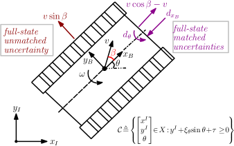
Figure 1: Illustration of the full-state matched and unmatched uncertainties for a tracked mobile robot in the presence of skidding and slipping, and description of the safe set ${\mathcal{C}}$ for Example 5.

$$\underbrace{\begin{bmatrix}\dot{x}^{I}\\ \dot{y}^{I}\\ \dot{\theta}\end{bmatrix}}_{\dot{x}}=\underbrace{\begin{bmatrix}0\\ 0\\ 0\end{bmatrix}}_{\hat{f}(x)}+\underbrace{\begin{bmatrix}\cos{\theta}&0\\ \sin{\theta}&0\\ 0&1\end{bmatrix}}_{\hat{g}(x)}\underbrace{\begin{bmatrix}v\\ w\end{bmatrix}}_{u}$$ (69)

where ${\begin{bmatrix}{x}^{I}&{y}^{I}\end{bmatrix}^{T}}$ is vehicle’s planar position with respect to the inertial frame ${I}$, $\theta$ is vehicle’s yaw angle, ${v}$ is its linear velocity and ${\omega}$ is the angular velocity.

A more complicated model lumps all of the unmodeled track-terrain interaction effects into terms that model a time-varying slip angle $\beta(t)$, a yaw rate uncertainty $d_{\theta}(t)$, and a longitudinal slip velocity ${d_{x_{B}}(t)}$ that accounts for slippage between the track treads and the supporting terrain [49], [50]:

$$\begin{bmatrix}\dot{x}^{I}\\ \dot{y}^{I}\\ \dot{\theta}\end{bmatrix}\!\!=\!\!\begin{bmatrix}\cos{\theta}&0\\ \sin{\theta}&0\\ 0&1\end{bmatrix}\!\!\begin{bmatrix}v\\ w\end{bmatrix}\!+\!\underbrace{\begin{bmatrix}\!v(\cos\gamma\!-\!\cos\theta)\!-\!d_{x_{B}}\cos{\theta}\\ \!v(\sin\gamma\!-\!\sin\theta)\!-\!d_{x_{B}}\sin{\theta}\\ \!d_{\theta}\end{bmatrix}}_{\Delta(t,x,u)},$$ (70)

where ${\gamma\!\triangleq\!\theta\!+\!\beta}$. Note that (70) is a nonlinear control affine system with the time-varying, state, and input-dependent uncertainty, like (20). This more advanced model, which still simplifies many physical effects, and has parameters that vary with vehicle speed and terrain characteristics, allows us to quantitatively analyze the effects of disturbances. In Fig. 1, note that a component of the slip, ${v\cos{\beta}-v}$, and the disturbance ${d_{x_{B}}}$ are parallel to the ${x_{B}}$-axis. These uncertainties affect the robot’s linear velocity, and their effect can be compensated by control $v$. Thus, these uncertainties are classified as full-state matched uncertainty/disturbance [51]. On the other hand, the second slip component, ${v\sin{\beta}}$, is perpendicular to ${x_{B}}$. It cannot be compensated by inputs ${v}$ or ${w}$; therefore, ${v\sin{\beta}}$ is a full-state unmatched uncertainty.

Continuing with this example, the left inverse of the input nominal input, $\hat{g}$ is

$$\hat{g}^{\dagger}(x) \!=\begin{bmatrix}\cos{\theta}&\sin{\theta}&0\\ 0&0&1\end{bmatrix},$$ (71)

which maps the full-state matched part of the uncertainty to the system input channel:

$$\begin{split}\hat{g}^{\dagger}(x){\Delta(t,x,u)}=\begin{bmatrix}v(\cos{\beta}-1)-d_{x_{B}}\\ d_{\theta}\end{bmatrix}\!,\end{split}$$ (72)

and the full-state matched uncertainty is obtained using (30):

$$\begin{split}\Delta_{m}(t,x,u)=\begin{bmatrix}v\cos{\theta}(\cos{\beta}-1)-d_{x_{B}}\cos{\theta}\\ v\sin{\theta}(\cos{\beta}-1)-d_{x_{B}}\sin{\theta}\\ d_{\theta}\end{bmatrix},\end{split}$$ (73)

and the full-state unmatched uncertainty, based on (31), is:

$$\begin{split}\Delta_{u}(t,x,u)=\begin{bmatrix}-v\sin{\theta}\sin{\beta}\\ v\cos{\theta}\sin{\beta}\\ 0\end{bmatrix},\end{split}$$ (74)

which is the observed value of vector ${v\sin{\beta}}$, the full-state unmatched uncertainty, in the inertial frame. $\Delta_{u}(t,x,u)$ is the lateral vehicle motion due to improperly modeled slip.

The sum ${\Delta_{m}(t,x,u)+\Delta_{u}(t,x,u)}$ is the compound uncertainty ${\Delta(t,x,u)}$ defined in (70). In summary, the uncertain unicycle model (70) with separated full-state matched and unmatched uncertainties, (72) and (74), is given by

$$\dot{x}\!=\!\hat{g}(x)\!\left(\!\!u\!+\!\!\begin{bmatrix}v(\cos{\beta}\!-\!1)\!-\!d_{x_{B}}\\ d_{\theta}\end{bmatrix}\!\right)\!\!+\!\!\!\begin{bmatrix}-v\sin{\theta}\sin{\beta}\\ v\cos{\theta}\sin{\beta}\\ 0\end{bmatrix}.$$ (75)

Next, we consider how the unicycle model uncertainty $\Delta$ (70) impacts the CBF constraint. For illustration, consider a safety constraint where the mobile robot must maintain a safe distance ${\tau\!\in\!\mathbb{R}^{+}_{0}}$ from an edge (e.g., a wall) aligned in the ${y}^{I}$ direction:

$$h(x)={y}^{I}+\xi_{\theta}\sin{\theta}+\tau,$$ (76)

where $\xi_{\theta}\!\in\!\mathbb{R}^{+}_{0}$, which determines the effect of the heading angle on safety, (see Fig. 1). This CBF choice results in

$$\begin{split}&L_{\hat{f}}h(x)=0,\ \ \ \ \ L_{\hat{g}}h(x)=\begin{bmatrix}\sin{\theta}&\xi_{\theta}\cos{\theta}\end{bmatrix}^{T},\\ &\frac{\partial h}{\partial x}\Delta(t\!,x,\!u)\!=\!v(\sin{\gamma}\!-\!\sin{\theta})\!-\!d_{x_{B}}\!\sin{\theta}\!+\!d_{\theta}\xi_{\theta}\cos{\theta},\end{split}$$ (77)

where the CBF ${h}$ has $\text{DRD}=\text{IRD}=1$.

Following Definition 1, we choose a simple extended class-$\mathcal{K}$ function: ${\alpha(h(x))\triangleq\alpha h(x),~{}\alpha\in\mathbb{R}^{+}}$. Note that $h$ is a valid CBF for the nominal system as ${L_{\hat{g}}h(x)\!\neq\!0}$, $\forall x\!\in\!X$; therefore, we have

$$v\sin{\theta}+\omega\xi_{\theta}\cos{\theta}\geq-\alpha({y}^{I}+\xi_{\theta}\sin{\theta}+\tau),\ \forall x\in\mathcal{C},$$ (78)

which is affine in the control input vector $u$.

To analyze the effect of uncertainty on safety, consider the CBF (21) under the uncertain unicycle model (70):

$$\begin{split}&\overbrace{v\sin{\theta}+\omega\xi_{\theta}\cos{\theta}+\alpha({y}^{I}+\xi_{\theta}\sin{\theta}+\tau)}^{\geq 0}\\ &~{}~{}~{}~{}~{}\geq-v(\sin{\gamma}-\sin{\theta})+d_{x_{B}}\sin{\theta}-d_{\theta}\xi_{\theta}\cos{\theta}.\end{split}$$ (79)

The left-hand side of (LABEL:eq:cbfununi) equals the inequality in (78), which is satisfied since $h$ is a valid CBF for the nominal system. The right-hand side of (LABEL:eq:cbfununi) quantifies the effect of uncertainty on safety: when it is positive (e.g., if the linear velocity ${v>0}$, heading angle lies in the interval ${-\pi/4<\theta<0}$, the slip angle lies in the range ${-\pi/4<\beta<0}$, ${d_{x_{B}}\leq 0}$, and ${d_{\theta}\leq 0}$, then the right-hand term will be positive), safety may be violated.

To address this robustness problem, the following section integrates the proposed uncertainty estimator, described in (38) and (39), with a quantifiable estimation error bound, derived in Lemma 2 in order to eliminate the full-state matched uncertainty. The error bound and unmatched uncertainty are integrated into the CBF and HOCBF conditions.

6 Uncertainty Estimation and Compensation-Based Robust CBFs

This section uses the active uncertainty attenuation capability of the proposed estimator to compensate uncertainty via an uncertainty estimation-based composite feedback controller. We show that this method provides provable safe controllers with CBFs and HOCBFs.

6.1 Uncertainty Estimation-Based Safety with CBFs

This subsection considers CBFs with relative degree one, i.e., IRD ${=1}$; therefore, from Assumption 3, DRD ${\geq 1}$.

To guarantee CBF robustness, we must consider uncertainty ${\Delta}$ in our analysis, even though it cannot be measured in practice. We address this issue by replacing ${\Delta}$ with the estimated uncertainty term ${\hat{\Delta}}$ and a lower bound on the estimation error ${{e}}$. The following theorem summarizes the robust safety assurances provided by uncertainty estimation and full-state matched uncertainty cancellation.

Theorem 4.

Consider system (20) with uncertainty ${\Delta}$ that includes full-state matched and unmatched components and satisfies Assumption 2, an uncertainty estimator and a feedback control law ${{u}=\bar{u}-\hat{g}^{\dagger}(x)\hat{\Delta}(t)}$ given in (38), (39), and (66), respectively. Let $h$ be a CBF for (20) on set ${\mathcal{C}\triangleq\left\{x\in X~{}|~{}h(x)\geq 0\right\}}$ such that ${\frac{\partial h}{\partial x}\neq 0}$ for all ${x\in\partial\mathcal{C}}$. Any Lipschitz continuous controller ${\bar{u}\!=\!\mathbf{\bar{k}}(x)}$ satisfying

$$\begin{split}L_{\hat{f}}h(x)+L_{\hat{g}}h(x)({\bar{u}-\hat{g}^{\dagger}(x)\hat{\Delta}(t)})+\dfrac{\partial h(x)}{\partial x}\hat{\Delta}(t)\\ -\left\|\frac{\partial h(x)}{\partial x}\right\|\bar{e}(t)\geq-\alpha(h(x))\end{split}$$ (80)

for all ${x\in\mathcal{C}}$ renders set ${\mathcal{C}}$ forward invariant: $x(0)\in\mathcal{C}\implies x(t)\in\mathcal{C},~{}\forall t\geq 0$.

Proof.

From (66) and (LABEL:syscon) the closed-loop system dynamics is:

$$\begin{split}\dot{x}=\hat{f}(x)+\hat{g}(x)\big{(}{\bar{u}-\hat{g}^{\dagger}(x)\hat{\Delta}(t)}\big{)}+\hat{\Delta}(t)+e(t).\end{split}$$ (81)

According to Theorem (1), safety is ensured with respect to set $\mathcal{C}$ by the CBF condition (7) assuming that IRD ${=1}$. Substituting (81) into (7) yields:

$$\begin{split}L_{\hat{f}}h(x)+L_{\hat{g}}h(x)\big{(}{\bar{u}-\hat{g}^{\dagger}(x)\hat{\Delta}(t)}\big{)}+\dfrac{\partial h(x)}{\partial x}\hat{\Delta}(t)\\ +\dfrac{\partial h(x)}{\partial x}e(t)\geq-\alpha(h(x)),~{}~{}\forall x\in\mathcal{C},\end{split}$$ (82)

where the estimation error $e$ is unknown. Thus ${\frac{\partial h(x)}{\partial x}e(t)}$ is also unknown. But, (62) upper bounds the estimation error. To obtain a sufficient CBF condition, we replace the unknown term in (82) with the lower bound ${\left(-\left\|\partial h(x)/\partial x\right\|\bar{e}(t)\right)}$:

$$L_{\hat{f}}h(x)+L_{\hat{g}}h(x)\big{(}{\bar{u}-\hat{g}^{\dagger}(x)\hat{\Delta}(t)}\big{)}+\dfrac{\partial h(x)}{\partial x}\hat{\Delta}(t)$$

$$~{}~{}~{}~{}~{}~{}~{}~{}~{}-\left\|\dfrac{\partial h(x)}{\partial x}\right\|\bar{e}(t)\geq-\alpha(h(x)),~{}\forall x\in\mathcal{C}$$

$$\quad\implies\dot{h}(t,x,u)\geq-\alpha(h(x)),~{}\forall x\in\mathcal{C},$$ (83)

which implies that ${x(t)\in\mathcal{C},~{}\forall t\geq 0}$ when ${x_{0}\in\mathcal{C}}$. ∎

Given a locally Lipschitz continuous desired controller $\mathbf{k_{d}}$, using Theorem 4, one can design a safe controller by solving the following uncertainty estimation and cancellation-based robust safety filter:

$$\begin{array}[]{lll}{\mathbf{\bar{k}^{*}}(x)=\ }\displaystyle\operatorname*{arg\,min}_{\bar{u}\in\mathbb{R}^{m}}\ \ \ \ {\|\bar{u}-\mathbf{k_{d}}(x)\|^{2}}\\[5.69054pt] ~{}~{}~{}~{}~{}~{}\textrm{s.t.}\ \ \ L_{\hat{f}}h(x)\!+\!L_{\hat{g}}h(x)\big{(}{\bar{u}-\hat{g}^{\dagger}(x)\hat{\Delta}(t)}\big{)}\!+\!\dfrac{\partial h(x)}{\partial x}\hat{\Delta}(t)\\[5.69054pt] ~{}~{}~{}~{}~{}~{}~{}~{}~{}~{}~{}~{}~{}~{}~{}~{}~{}~{}~{}-\left\|\dfrac{\partial h(x)}{\partial x}\right\|\bar{e}(t)\geq-\alpha(h(x))\\[8.53581pt] ~{}~{}~{}~{}~{}~{}~{}~{}~{}~{}~{}~{}~{}\bar{u}-\hat{g}^{\dagger}(x)\hat{\Delta}(t)\in U,\end{array}$$

which can be implemented as an efficient QP.

Note that the robust CBF condition (6.1) explicitly depends on the time-varying upper error bound, ${\bar{e}}$. A similar method was initially used in [27] to address robustness against unmodeled system dynamics by estimating the effect of the disturbance on the CBF requirement. While safety was guaranteed in that prior work, uncertainty compensation via estimation was not considered, and the proposed safety filter [27] may perform poorly.

By Lemma 1, the estimation error dynamics is ISS, with ISS Lyapunov function ${V_{e}}$ (see (48)). Using this stability property, we incorporate the uncertainty estimator (38), (39) into the CBF construction with the augmentation of the existing CBF. In particular, we modify the CBF $h$ to provide robustness against estimation error $e$:

$$h_{V}(x,e)\triangleq h(x)-\sigma_{V}V_{e}(e),$$ (84)

$$\mathcal{C}_{V}\triangleq\left\{[x~{}e]^{T}\in X\!\times\!\mathbb{R}^{n}~{}|~{}h_{V}(x,e)\geq 0\right\},$$ (85)

where ${~{}\sigma_{V}\in\mathbb{R}^{+}}$. Since ${V_{e}}$ is a Lyapunov function, ${\mathcal{C}_{V}}$ is a subset of safe set ${\mathcal{C}\triangleq\left\{x\in X~{}|~{}h(x)\geq 0\right\}}$. We assume that ${\frac{\partial h_{V}}{\partial x_{e}}\neq 0}$, for all ${\partial{\mathcal{C}_{V}}}$, where ${x_{e}\triangleq[x~{}e]^{T}}$.

The following theorem uses the estimator dynamics to relate the controllers designed for nominal system safety to the safety of the uncertain system. Note that for Theorem 5 we use a specific extended class-${\mathcal{K}_{\infty,e}}$ function, ${\alpha(h(x))=\alpha h(x)}$, i.e., ${\alpha\in\mathbb{R}^{+}}$, for simplicity. The proof drops function arguments for convenience.

Theorem 5.

Under the same assumptions of Theorem 4, let $h_{V}$ be a CBF for (20) on ${\mathcal{C}_{V}}$. Consider the ISS Lyapunov function of the uncertainty estimator dynamics with the inequality in (54): ${\dot{V}_{e}\leq-2\mu_{e}\|e\|^{2}+\gamma(\|\delta_{L}\|)}$, which is the result of Lemma 1, and a constant ${\alpha_{h}\in\mathbb{R}^{+}}$ such that

$$\mathcal{E}\triangleq 2\sigma_{V}\mu_{e}-\dfrac{\sigma_{V}\alpha_{h}}{2}>0,$$ (86)

then, any Lipschitz continuous controller ${\bar{u}\!=\!\mathbf{\bar{k}}(x)}$ satisfying

$$\begin{split}L_{\hat{f}}h(x)+L_{\hat{g}}h(x)\big{(}\bar{u}-\hat{g}^{\dagger}(x)\hat{\Delta}(t)\big{)}+\dfrac{\partial h(x)}{\partial x}\hat{\Delta}(t)\\ \geq-\alpha_{h}h(x)+\dfrac{1}{4\mathcal{E}}\left\|\dfrac{\partial h(x)}{\partial x}\right\|^{2}+\sigma_{V}\gamma(\|\delta_{L}\|),\end{split}$$ (87)

for all ${x_{e}\in\mathcal{C}_{V}}$ renders the set ${\mathcal{C}_{V}}$ forward invariant: ${x_{e}(0)\in\mathcal{C}_{V}\implies x_{e}(t)\in\mathcal{C}_{V}}$.

Proof.

Our goal is to prove that ${\dot{h}_{V}\geq-\alpha_{h}h_{V},~{}\forall t\geq 0}$ which implies that ${\dot{h}\geq-\alpha_{h}h,~{}\forall t\geq 0}$. The time derivative of ${h_{V}}$ in (84) satisfies:

$$\begin{split}\dot{h}_{V}&\!=\!\dot{h}-\sigma_{V}\dot{V}_{e}\!\geq\!\dot{h}-\sigma_{V}(-2\mu_{e}\|e\|^{2}+\gamma(\|\delta_{L}\|))\\ &\!=\!L_{\hat{f}}h\!+\!L_{\hat{g}}h({\bar{u}\!-\!\hat{g}^{\dagger}\hat{\Delta}})\!+\!\dfrac{\partial h}{\partial x}\hat{\Delta}\!+\!\dfrac{\partial h}{\partial x}e\\ &~{}~{}~{}~{}~{}~{}~{}~{}+2\sigma_{V}\mu_{e}\|e\|^{2}\!-\!\sigma_{V}\gamma(\|\delta_{L}\|)\\ &\!=\!L_{\hat{f}}h\!+\!L_{\hat{g}}h({\bar{u}\!-\!\hat{g}^{\dagger}\hat{\Delta}})\!+\!\dfrac{\partial h}{\partial x}\hat{\Delta}\!+\!\dfrac{\partial h}{\partial x}e-\sigma_{V}\gamma(\|\delta_{L}\|)\\ &~{}~{}+\underbrace{\left(2\sigma_{V}\mu_{e}-\frac{\sigma_{V}\alpha_{h}}{2}\right)}_{=\mathcal{E}}\|e\|^{2}+\frac{\sigma_{V}\alpha_{h}}{2}\|e\|^{2}\\ &\!=\!L_{\hat{f}}h\!+\!L_{\hat{g}}h({\bar{u}\!-\!\hat{g}^{\dagger}\hat{\Delta}})\!+\!\dfrac{\partial h}{\partial x}\hat{\Delta}-\sigma_{V}\gamma(\|\delta_{L}\|)\\ &~{}~{}+\left(\sqrt{\mathcal{E}}e+\dfrac{1}{2\sqrt{\mathcal{E}}}{\frac{\partial h}{\partial x}}\right)^{2}-\dfrac{1}{4\mathcal{E}}\left\|\dfrac{\partial h}{\partial x}\right\|^{2}+\frac{\sigma_{V}\alpha_{h}}{2}\|e\|^{2}\\ &\!\geq\!\underbrace{L_{\hat{f}}h\!+\!L_{\hat{g}}h({\bar{u}\!-\!\hat{g}^{\dagger}\hat{\Delta}})\!+\!\dfrac{\partial h}{\partial x}\hat{\Delta}\!-\!\dfrac{1}{4\mathcal{E}}\left\|\dfrac{\partial h}{\partial x}\right\|^{2}\!\!-\!\sigma_{V}\gamma(\|\delta_{L}\|)}_{\geq-\alpha_{h}h}\\ &~{}~{}~{}~{}~{}~{}~{}~{}~{}~{}~{}+\dfrac{\sigma_{V}\alpha_{h}\|e\|^{2}}{2}\\ &\implies\dot{h}_{V}\geq-\alpha_{h}h+\dfrac{\sigma_{V}\alpha_{h}\|e\|^{2}}{2}=-\alpha_{h}h_{V}\end{split}$$

This result guarantees that ${x_{e}(t)\in\mathcal{C}_{V}}$, ${\forall t\geq 0}$ if ${x_{e}(0)\in\mathcal{C}_{V}}$, which implies ${h(x(t))\geq 0}$, ${\forall t\geq 0}$.

The second proof line uses the upper bound of ${V_{e}}$ described in Eq. (54) of Lemma 1. Note that ${\dot{h}}$ is given in (82): it is used in the third proof line. The next line uses a square to define a new lower bound. Finally, we obtain the main statement using the condition in the theorem. ∎

Remark 8.

Condition ${2\sigma_{V}\mu_{e}\!-\!\frac{\sigma_{V}\alpha_{h}}{2}\!>\!0\!\iff\!\lambda_{\rm min}(\Lambda)\!>\!\alpha_{h}}$ requires the uncertainty estimation dynamics represented by $\lambda_{\rm min}(\Lambda)$ to be faster than the exponential rate of the CBF constraint, which is characterized by $\alpha_{h}$. For a given uncertainty estimator, it is possible to select an $\alpha_{h}$ value that is sufficiently small in practical applications.

Remark 9.

For Theorem 5, we require ${x_{e}(0)\in\mathcal{C}_{V}}$. This condition requires ${h(0)\geq\sigma_{V}V_{e}(0)}$, which is a more stringent condition than ${x_{0}\in\mathcal{C}}$. This conservatism can be minimized by reducing the initial estimation error ${e(0)}$, which results in a smaller value of ${\sigma_{V}V_{e}(0)}$.

Remark 10.

The safety condition (87) is not explicitly affected by the time-varying estimation error $e$, whereas (80) depends on it. Therefore, Theorem 5 gives design flexibility even if the upper bound ${\delta_{b}}$ is unknown, as the upper bound of $\|e\|$, ${\bar{e}(t)}$, given in (59) explicitly depends on ${\delta_{b}}$.

Then, given a CBF $h$, $\alpha_{h}$, ${\delta_{L}}$, and ${\Lambda}$ for system (20), the pointwise set of all control values that satisfy robust safety condition (87) is defined as

$$\begin{split}K_{\text{UE}}(x)\!\triangleq\!\bigg{\{}\!{u}\!\in\!U\big{|}L_{\hat{f}}h\!+\!L_{\hat{g}}h({\bar{u}\!-\!\hat{g}^{\dagger}\hat{\Delta}(t)})\!+\!\dfrac{\partial h}{\partial x}\hat{\Delta}(t)\\ \!\geq\!-\alpha_{h}h(x)+\dfrac{1}{4\mathcal{E}}\left\|\dfrac{\partial h(x)}{\partial x}\right\|^{2}+\sigma_{V}\gamma(\|\delta_{L}\|)\bigg{\}}.\end{split}$$ (88)

Finally, given a desired controller ${\mathbf{k_{d}}}$, to design an optimal robust safe controller ${{\bar{u}^{*}}\!=\!\mathbf{\bar{k}^{*}}(x),~{}\mathbf{\bar{k}^{*}}\!:\!X\!\to\!\mathbb{R}^{m}}$ satisfying ${u^{*}\!=\!\big{(}\bar{u}^{*}\!-\!\hat{g}^{\dagger}(x)\hat{\Delta}(t)\big{)}\!\in\!K_{\text{UE}}(x)}$, we define an uncertainty estimation-based robust safety filter, UE-CBF-QP:

$$\begin{array}[]{lll}{\mathbf{\bar{k}^{*}}(x)=\ }\displaystyle\operatorname*{arg\,min}_{\bar{u}\in\mathbb{R}^{m}}\ \ \ \ {\|\bar{u}-\mathbf{k_{d}}(x)\|^{2}}\\[5.69054pt] ~{}~{}~{}~{}~{}~{}\textrm{s.t.}\ \ \ L_{\hat{f}}h(x)\!+\!L_{\hat{g}}h(x)\big{(}\bar{u}-\hat{g}^{\dagger}(x)\hat{\Delta}(t)\big{)}\!+\!\dfrac{\partial h(x)}{\partial x}\hat{\Delta}(t)\\[2.84526pt] ~{}~{}~{}~{}~{}~{}~{}~{}~{}~{}~{}~{}~{}~{}~{}\geq-\alpha_{h}h(x)\!+\!\dfrac{1}{4\mathcal{E}}\left\|\dfrac{\partial h(x)}{\partial x}\right\|^{2}+\sigma_{V}\gamma(\|\delta_{L}\|)\\[8.53581pt] ~{}~{}~{}~{}~{}~{}~{}~{}~{}~{}~{}~{}~{}~{}\bar{u}-\hat{g}^{\dagger}(x)\hat{\Delta}(t)\in U,\end{array}$$

which is depicted in Fig. 2.

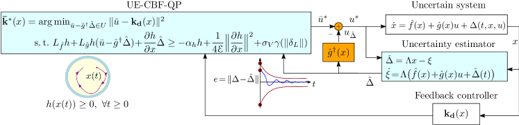
Figure 2: Block diagram of the uncertainty estimator-based safe control framework. Augmenting a given, and potentially unsafe, controller with an error-bounded uncertainty estimator and a safety filter guarantees that uncertain system states remain in a subset of the safe set.

6.2 Uncertainty Estimation-Based Safety with HOCBFs

This subsection extends the uncertainty estimation-based robust safe control design method to HOCBFs in the presence of unmatched uncertainty under Assumption 3.

Suppose IRD ${=r}$ and DRD ${=r-1}$, and ${r\geq 2}$, the higher-order time derivatives of $h$ with respect to the system dynamics (20) are given in (LABEL:eq:hocbfder1). We modify (LABEL:eq:squphi) with respect to the uncertain system (20), which results in:

$$\begin{split}&\phi_{0}(x)\triangleq h(x),\\ &\phi_{1}(x)\triangleq\dot{h}(x)+\alpha_{1}({\phi}_{0}(x)),\\ &\phi_{r-1}(t,x,u)\triangleq\frac{\partial L_{\hat{f}}^{r-2}h(x)}{\partial x}{\Delta}(t,x,u)\\ &~{}~{}~{}~{}+\underbrace{L_{\hat{f}}^{r-1}h(x)+\sum_{i=1}^{r-1}L_{\hat{f}}^{i-1}(\alpha_{r-i}\circ{\phi}_{r-i-1})(x)}_{\triangleq\Psi(x)}.\end{split}$$ (89)

Note that, $\Delta$ first appears in ${\phi_{r-1}}$ as it depends on ${{h}^{r-1}}$, which depends on $\Delta$; see (LABEL:eq:hocbfder1). We also define the following sets and their intersections for ${i\!\in\!\{0,1,\ldots,r\!-\!1\}}$:

$$\begin{split}\mathcal{C}_{i}&\triangleq\{(t,x,u)\in\mathbb{R}^{+}_{0}\!\times\!X\!\times\!U:{\phi}_{i}(t,x,u)\geq 0\},\\ \mathcal{C}&\triangleq\bigcap_{i=0}^{r-1}\mathcal{C}_{i},\end{split}$$ (90)

which is a control input-dependent and time-varying set. Then, according to Theorem (2), safety is ensured with respect to the set $\mathcal{C}$ by the robust HOCBF condition:

$$\dot{\phi}_{r-1}(t,x,u)\geq-\alpha_{r}\left({\phi}_{r-1}(t,x,u)\right),\ \forall x\in\mathcal{C},$$ (91)

which can be expressed in terms of the constraint function $h$:

$$\begin{split}&L_{\hat{f}}\Psi(x)+L_{\hat{g}}\Psi(x)u+\frac{\partial\Psi(x)}{\partial x}{\Delta}(t,x,u)\\ &\!+\!\left(\hat{f}(x)\!+\!\hat{g}(x)u\!+\!{\Delta}(t,x,u)\!\right)^{T}\underbrace{\frac{\partial}{\partial x}\!\!\left(\!\frac{\partial L_{\hat{f}}^{r-2}h(x)}{\partial x}\!\right)\!}_{\triangleq\mathcal{F}(x)}{\Delta}(t,x,u)\\ &\!+\!\frac{\partial L_{\hat{f}}^{r-2}h(x)}{\partial x}~{}\dfrac{d}{dt}{\Delta}(t,x,u)\\ &\!\geq\!-\alpha_{r}\left(\Psi(x)+\frac{\partial L_{\hat{f}}^{r-2}h(x)}{\partial x}{\Delta}(t,x,u)\right),\ \forall x\in\mathcal{C},\end{split}$$ (92)

where ${\alpha_{r}\!\in\!\mathcal{K}_{\infty,e}}$, ${\mathcal{F}\!:\!X\!\to\!\mathbb{R}^{n\times n}}$. And, from Assumption 2 we have

$$\frac{\partial L_{\hat{f}}^{r-2}h(x)}{\partial x}~{}\dfrac{d}{dt}{\Delta}(t,x,u)\geq-\left\|\frac{\partial L_{\hat{f}}^{r-2}h(x)}{\partial x}\right\|\delta_{L},$$ (93)

for all ${(t,\!x,\!u)\!\in\!\mathbb{R}^{+}_{0}\!\times\!X\!\times\!U}$.

Like Theorem 4, we replace $\Delta$ with ${\hat{\Delta}\!+\!e}$, and $u$ with ${\bar{u}\!-\!\hat{g}^{\dagger}\hat{\Delta}}$ in (LABEL:eq:hocbfproofmod) to integrate the uncertainty estimator into the robust safety constraint. This process results in the following error-dependent HOCBF condition similar to (6.1):

$$\begin{split}&L_{\hat{f}}\Psi(x)+L_{\hat{g}}\Psi(x)\big{(}\bar{u}-\hat{g}^{\dagger}(x)\hat{\Delta}(t)\big{)}+\frac{\partial\Psi(x)}{\partial x}\hat{\Delta}(t)\\ &+\big{(}\hat{f}(x)+\hat{g}(x)\big{(}\bar{u}-\hat{g}^{\dagger}(x)\hat{\Delta}(t)\big{)}+\hat{\Delta}(t)\big{)}^{T}\mathcal{F}(x)\hat{\Delta}(t)\\ &\!-\!\bar{e}(t)\big{\|}\big{(}\hat{f}(x)+\hat{g}(x)\big{(}\bar{u}-\hat{g}^{\dagger}(x)\hat{\Delta}(t)\big{)}+\hat{\Delta}(t)\big{)}^{T}\mathcal{F}(x)\big{\|}\\ &-\Bigg{\|}\frac{\partial L_{\hat{f}}^{r-2}h(x)}{\partial x}\Bigg{\|}\delta_{L}-\Omega(t,x,e)\\ &\geq\!-\alpha_{r}\!\left(\!\!\Psi(x)\!+\!\frac{\partial L_{\hat{f}}^{r-2}h(x)}{\partial x}\hat{\Delta}(t)\!-\!\left\|\frac{\partial L_{\hat{f}}^{r-2}h(x)}{\partial x}\right\|\bar{e}(t)\!\!\right),\end{split}$$ (94)

where we define a function: ${\Omega\!:\!\mathbb{R}^{+}_{0}\!\times\!X\!\times\!\mathbb{R}^{n}\!\to\!\mathbb{R}^{n}}$ for notational simplicity as

$$\Omega(t,\!x,\!e)\!\triangleq\!\bigg{\|}\frac{\partial\Psi(x)}{\partial x}\bigg{\|}\bar{e}(t)+\big{\|}\mathcal{F}(x)\big{\|}\big{\|}\hat{\Delta}(t)\big{\|}\bar{e}(t)+\big{\|}\mathcal{F}(x)\big{\|}\bar{e}^{2}(t).$$

Note that we use the induced matrix 2-norm, which satisfies the submultiplicative property, in (LABEL:eq:hocbfeineqfex) to bound the matrices.

Theorem 6.

Let the sufficiently differentiable function ${h}$ be an HOCBF for the uncertain model (20) on set ${\mathcal{C}}$, constructed in (90). Consider an uncertainty ${\Delta}$ of the form (26) that satisfies both Assumption 3 and Assumption 2, an uncertainty estimator with an associated ISS Lyapunov function $V_{e}$ that satisfies (54), and a feedback control law ${{u}=\bar{u}-\hat{g}^{\dagger}(x)\hat{\Delta}(t)}$. Then, any Lipschitz continuous controller ${\bar{u}\!=\!\mathbf{\bar{k}}(x)}$ satisfying (LABEL:eq:hocbfeineqfex) renders the set ${\mathcal{C}}$ forward invariant: ${\left(x(0)\!\in\!\mathcal{C}\implies x(t)\!\in\!\mathcal{C}\right)\implies h(x(t))\!\geq\!0,\forall t\geq 0}$.

Proof.

We follow the same steps described in the proof of Theorem 4. We replace the unknown terms with their lower bounds to obtain a sufficient HOCBF condition. Since inequality in (LABEL:eq:hocbfeineqfex) $\implies$ (LABEL:eq:hocbfproofmod), we have that the uncertain system is safe with respect to set $\mathcal{C}$ by Theorem 2. ∎

Then, given a desired controller ${\mathbf{k_{d}}}$, to design a controller ${\mathbf{\bar{k}}\!:\!X\!\to\!\mathbb{R}^{m}}$ satisfying (LABEL:eq:hocbfeineqfex), we define an uncertainty estimation-based robust UE-HOCBF safety filter:

$$\begin{array}[]{lll}{\mathbf{\bar{k}^{*}}(x)=\ }\displaystyle\operatorname*{arg\,min}_{\bar{u}\in\mathbb{R}^{m}}\ \ \ \ {\|\bar{u}-\mathbf{k_{d}}(x)\|^{2}}\\[11.38109pt] ~{}~{}~{}~{}\textrm{s.t.}\ \ \bar{e}(t)\big{\|}\big{(}\hat{f}(x)\!+\!\hat{g}(x)\big{(}\bar{u}\!-\!\hat{g}^{\dagger}(x)\hat{\Delta}(t)\big{)}\!+\!\hat{\Delta}(t)\big{)}^{T}\mathcal{F}(x)\big{\|}\\[2.84526pt] ~{}~{}~{}~{}~{}~{}~{}~{}~{}~{}~{}~{}~{}~{}~{}~{}~{}~{}~{}~{}~{}~{}~{}~{}~{}~{}~{}~{}~{}~{}\leq\tilde{a}(t,x)\bar{u}+\tilde{b}(t,x,e)\\[2.84526pt] ~{}~{}~{}~{}~{}~{}~{}~{}~{}~{}~{}\bar{u}-\hat{g}^{\dagger}(x)\hat{\Delta}(t)\in U,\end{array}$$

where

$$\begin{split}&\tilde{a}(t,x)\triangleq L_{\hat{g}}\Psi(x)\!+\!\big{(}\hat{g}^{T}(x)\mathcal{F}(x)\hat{\Delta}(t)\big{)}^{T},\\ &\tilde{b}(t,x,e)\triangleq L_{\hat{f}}\Psi(x)\!+\!L_{\hat{g}}\Psi(x)\big{(}\!-\hat{g}^{\dagger}(x)\hat{\Delta}(t)\big{)}\!+\!\frac{\partial\Psi(x)}{\partial x}\hat{\Delta}(t)\\ &+\big{(}\hat{f}(x)+\hat{g}(x)\big{(}-\hat{g}^{\dagger}(x)\hat{\Delta}(t)\big{)}+\hat{\Delta}(t)\big{)}^{T}\mathcal{F}(x)\hat{\Delta}(t)\\ &-\Bigg{\|}\frac{\partial L_{\hat{f}}^{r-2}h(x)}{\partial x}\Bigg{\|}\delta_{L}-\Omega(t,x,e)\\ &+\alpha_{r}\!\left(\!\!\Psi(x)\!+\!\frac{\partial L_{\hat{f}}^{r-2}h(x)}{\partial x}\hat{\Delta}(t)\!-\!\left\|\frac{\partial L_{\hat{f}}^{r-2}h(x)}{\partial x}\right\|\bar{e}(t)\!\!\right),\end{split}$$ (95)

The sufficient HOCBF condition (LABEL:eq:hocbfeineqfex) is not affine in the control $\bar{u}$. Thus, the UE-HOCBF optimization problem is not a QP. However, we show next how to integrate the HOCBF condition into a second-order cone program (SOCP) [52]. To make the objective function linear, we convert the quadratic cost to epigraph form by adding a new variable: ${\rho\!\in\!\mathbb{R}}$:

$$\begin{array}[]{llll}{\mathbf{\bar{k}^{*}}(x)=\ }\displaystyle\operatorname*{arg\,min}_{\bar{u}\in\mathbb{R}^{m},~{}\rho\in\mathbb{R}}\ \ \ \ {\rho}\\[11.38109pt] ~{}~{}~{}~{}\textrm{s.t.}\ \ \bar{e}(t)\big{\|}\big{(}\hat{f}(x)\!+\!\hat{g}(x)\big{(}\bar{u}\!-\!\hat{g}^{\dagger}(x)\hat{\Delta}(t)\big{)}\!+\!\hat{\Delta}(t)\big{)}^{T}\mathcal{F}(x)\big{\|}\\[2.84526pt] ~{}~{}~{}~{}~{}~{}~{}~{}~{}~{}~{}~{}~{}~{}~{}~{}~{}~{}~{}~{}~{}~{}~{}~{}~{}\leq\tilde{a}(t,x)\bar{u}+\tilde{b}(t,x,e)\\[2.84526pt] ~{}~{}~{}~{}~{}~{}~{}~{}~{}\|\bar{u}-\mathbf{k_{d}}(x)\|^{2}\leq\rho\\[2.84526pt] ~{}~{}~{}~{}~{}~{}~{}~{}~{}\bar{u}-\hat{g}^{\dagger}(x)\hat{\Delta}(t)\in U,\end{array}$$

where the constraint ${\|\bar{u}-\mathbf{k_{d}}(x)\|^{2}\leq\rho}$ is a rotated second-order cone constraint; therefore, we can put this constraint into a standard second-order cone form:

$$\left\|\begin{bmatrix}2(\bar{u}-\mathbf{k_{d}}(x))\\ \rho-1\end{bmatrix}\right\|\leq\rho+1.$$ (96)

The UE-HOCBF-SOCP is the solution to optimization problem above with the second constraint replaced by (96). The UE-HOCBF-SOCP guarantees forward invariance of ${\mathcal{C}}$.

SOCP-CBF-based safety filters have been proposed for several robust safety-critical control problems [53, 54, 55]. In [40], the authors provide a sufficient condition for local Lipschitz continuity of the controller resulting from an SOCP-based safety filter.

Remark 11.

Specifically, if ${\mathcal{F}(x)\hat{g}(x)\equiv 0}$, the left-hand side of the inequality in the UE-HOCBF safety filter becomes independent of $\bar{u}$, and the optimization problem reduces to a QP. More specifically, suppose that ${\mathcal{F}(x)\equiv 0}$, then the constraint can be integrated into an uncertainty estimation-based QP, UE-HOCBF-QP:

$${\labelOP{opt:robHOCBFQP}}$$

Furthermore, if ${\mathcal{F}(x)\hat{g}(x)\equiv 0}$, we can extend Theorem 5 to HOCBFs. In order to achieve this objective, we need to modify ${\phi_{r-1}}$ and its 0-superlevel set to provide robustness against estimation error $e$, analogous to (84):

$$\phi_{r-1}^{V}(t,x_{e},u)\triangleq\phi_{r-1}(t,x,u)\!-\!\sigma_{V}V_{e}(e),~{}\sigma_{V}\!\in\!\mathbb{R}^{+},$$

$$\mathcal{C}_{r-1}^{V}\!\triangleq\!\left\{(t,\!x_{e},\!u)\!\in\!\mathbb{R}^{+}_{0}\!\times\!X\!\times\!\mathbb{R}^{n}\!\times\!U~{}|~{}\phi_{r-1}^{V}(t,\!x_{e},\!u)\!\geq\!0\right\},$$

which is a subset of ${\mathcal{C}_{r-1}}$. Then, one can easily follow the same steps in Theorem 5 and its proof.

Remark 12.

In order to compensate the mismatch between the nominal model and the uncertain system dynamics, we subtract the estimated uncertainty from the UE-CBF-QP and UE-HOCBF-SOCP outputs, as given in equation (66). This modification is for closed-loop control performance improvement only; thus, it is not related to safety. However, since it is a part of feedback control, it appears in the CBF constraints, as seen from the QPs. Therefore, one can remove ${-\hat{g}^{\dagger}(x)\hat{\Delta}(t)}$ from the composite control law (66). In this scenario, we only need to replace ${\mathbf{\bar{k}}(x)-\hat{g}^{\dagger}(x)\hat{\Delta}(t)}$ with ${\mathbf{\bar{k}}(x)}$ between equations (66) and (LABEL:opt:robHOCBFQP).

7 Elastic Actuator with Matched and Unmatched Uncertainties

We first demonstrate our robust HOCBF method on a simulated elastic actuator problem characterized by both full-state matched and unmatched uncertainty.

Consider a flexible-joint mechanism, adopted from [56] (Example 6.10), whose dynamics take the form (20):

$$\begin{split}&\underbrace{\begin{bmatrix}\dot{x}_{1}\\ \dot{x}_{2}\\ \dot{x}_{3}\\ \dot{x}_{4}\\ \end{bmatrix}}_{\dot{x}}=\underbrace{\begin{bmatrix}x_{2}\\ \dfrac{M\bar{g}L}{I_{L}}\sin{{x}_{1}}\!-\!\dfrac{k}{I_{L}}({x}_{1}-{x}_{3})\\ x_{4}\\ \dfrac{k}{J_{m}}({x}_{1}-{x}_{3})\end{bmatrix}}_{\hat{f}(x)}+\underbrace{\begin{bmatrix}0\\ 0\\ 0\\ \frac{1}{J_{m}}\end{bmatrix}}_{\hat{g}(x)}u\\ &\!+\!\!\overbrace{\underbrace{\begin{bmatrix}0\\ \dfrac{-({M\bar{g}L}\sin{{x}_{1}}\!-\!{k}({x}_{1}-{x}_{3}))}{3I_{L}}+0.1\\ 0\\ \dfrac{k({x}_{1}\!-\!{x}_{3})}{4J_{m}}\!-\!0.2\end{bmatrix}}_{\Delta f(x)}\!\!+\!\!\underbrace{\begin{bmatrix}0\\ 0\\ 0\\ \dfrac{1}{4J_{m}}\end{bmatrix}}_{\Delta g(x)}u}^{\Delta(x,u)\triangleq[\Delta_{1}~{}\Delta_{2}(x)~{}\Delta_{3}~{}\Delta_{4}(x,u)]^{T}},\end{split}$$ (100)

where ${{x}_{1},{x}_{3}}$ are the joint angles of the actuator, ${J_{m}}$ is the motor rotational inertia, ${k}$ is the torsional spring stiffness, $M$ is the load’s mass, ${I_{L}}$ is the load rotational inertia, $L$ is the eccentricity of the load’s center of mass, $\bar{g}$ is the gravitational constant, and $u$ is the motor torque. The uncertainty takes the form (22), and ${\Delta_{2}(x)\perp\operatorname{Range}(\hat{g}(x))}$. We consider the following control input set:

$$U\triangleq\left\{u\in\mathbb{R}:-u_{\rm max}\leq u\leq u_{\rm max}\right\},$$

where ${u_{\rm max}\in\mathbb{R}^{+}_{0}}$. We obtain ${\hat{g}^{\dagger}}$ from (19) as

$$\hat{g}^{\dagger}(x)=\begin{bmatrix}0&0&0&J_{m}\end{bmatrix},$$

which yields the full-state matched and unmatched uncertainty using (LABEL:syscon) as

$$\begin{split}{\Delta_{m}}(x,u)&=\Delta_{4}(x,u);\\ {\Delta_{u}}(x)&=\Delta_{2}(x).\end{split}$$

To synthesize a desired feedback controller, we choose a control Lyapunov function (CLF):

$$V(x)=x_{4}-x_{4d})^{2},$$

which embodies the tracking requirement for state ${x_{4}}$, where ${x_{4d}(t)\in\mathbb{R}}$ is the desired trajectory. This CLF choice yields the min-norm controller:

$$\mathbf{k_{d}}(x)\!=\!\begin{cases}\!\!-\dfrac{\overbrace{L_{f}V(x)\!+\!\lambda_{V}V(x)}^{\triangleq\varsigma(x)}}{\|L_{g}V(x)\|^{2}}L_{g}V^{T}(x)&\!\!\!\!\text{ if }\varsigma(x)\!>\!0\\ 0&\!\!\!\!\text{ if }\varsigma(x)\!\leq\!0\end{cases}$$

which is the solution of the CLF-QP [14] with ${\lambda_{V}\in\mathbb{R}^{+}}$.

We choose a CBF:

$$h(x)=x_{2}-c_{q}x_{3},$$

where ${c_{q}\in\mathbb{R}}$. The CBF ${h}$ has IRD of 2, i.e., ${r=2}$ in (LABEL:eq:hocbfder1), and DRD of 1. This uncertainty structure and CBF choice satisfies Assumption 3. We use an HOCBF framework. From (LABEL:eq:secphi) and (LABEL:eq:hocbfproofmod) we have

$$\begin{split}&\phi_{0}(x)=x_{2}-c_{q}x_{3},\\ &\phi_{1}(x)\!=\!\Delta_{2}(x)\\ &\!+\!\underbrace{\dfrac{{M\bar{g}L\sin{{x}_{1}}\!-\!k({x}_{1}\!-\!{x}_{3})}}{I_{L}}\!-\!c_{q}x_{4}\!+\!\alpha_{1}(x_{2}\!-\!c_{q}x_{3})}_{\Psi(x)},\\ &\mathcal{F}(x)\equiv 0.\end{split}$$

Since ${\mathcal{F}(x)\equiv 0}$, we use an UE-HOCBF-QP as a safety filter. Substituting ${\phi_{0},~{}\phi_{1}}$ into (LABEL:eq:qcqpparam) yields an affine HOCBF condition for the actuator system for some ${\alpha_{2}\in\mathcal{K}_{\infty,e}}$.

The simulation parameters are given in Table 1.

$m=0.5\ [kg]$	$x_{4d}=0$
$\bar{g}=9.81\ [m/s^{2}]$	$x(0)=[0~{}0.5~{}0~{}\!-0.2]^{T}$
$I_{L}=0.5\ [kgm^{2}]$	$u_{\rm max}=0.2\bar{g}$
$J_{m}=0.1\ [kgm^{2}]$	$c_{q}=-2$
$k=0.25\ [Nm/{rad}]$	$\lambda_{V}=10$
$L=0.04\ [{m}]$	$\alpha_{1}(h)=2h;~{}~{}\alpha_{2}(h)=2h$

Table 1: Simulation parameters for the elastic actuator example.

To obtain bounding constants ${\delta_{L},\delta_{b}}$ for the problem’s uncertainty, we simulate numerous scenarios, resulting in ${\delta_{L}=1,~{}\delta_{b}=0.9}$. We choose ${\Lambda=\operatorname{diag}(5,5,5,5)}$ in order to reach a small estimation error: ${\mu_{e}\triangleq\frac{\lambda_{\rm min}}{4}=1.25}$.

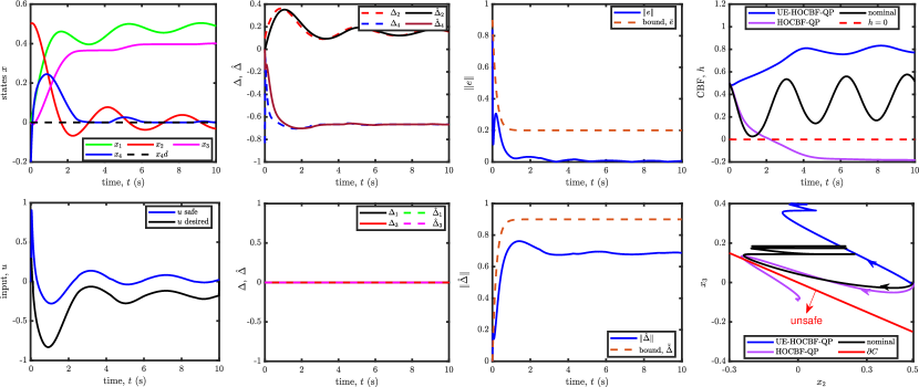
Figure 3: Simulations for the uncertain elastic actuator. (Left) (Top) Plots of states and reference tracking of the uncertain system operating under the UE-HOCBF-QP. (Bottom) The values of the safe control input, $u$ safe, and the desired input, $u$ desired, vs. time. (Center-left) The proposed uncertainty estimator can effectively estimate actual modelling uncertainties within the quantified bounds. Because of ${\hat{\Delta}(0)=\bf 0}$ and ${\Delta_{1}\equiv 0,~{}\Delta_{3}\equiv 0}$, the estimator results in zero for these uncertainty components. (Center-right) The estimation error (Top) and output (Bottom) with the theoretical bounds which are satisfied. (Right) (Top) The value of CBF $h$ vs. time and trajectory of the system with the boundary of the safe set (Bottom). The proposed UE-HOCBF-QP safety filter maintains safety in the presence of unmodelled dynamics. While HOCBF-QP satisfies safety for the nominal system, it leaves the safe set with the uncertain system.

Data from the simulated system (100 Hz sampling rate) are presented in Fig. 3. With the HOCBF-QP controller, the abstract nominal system, i.e., the elastic actuator dynamics without uncertainty, remains safe. But safety violations occur in the presence of unmodelled system dynamics. Note that the HOCBF-QP results in an unsafe system, whereas the system remains safe with our proposed method. Fig. 3 also demonstrates that the proposed uncertainty estimator effectively estimates actual modeling uncertainties within the quantified bounds. We chose ${H=\operatorname{diag}(1,1,1,1)}$ to solve Lyapunov equation (58).

8 Experimental Validation of Mobile Robot Example

We conducted an experimental test on an unmanned ground mobile robot. The example is explained in Section 5 models the GVR-Bot, tracked vehicle, see Fig. 4. For the test vehicle and onboard computation details, see Section IV in [57]. We conducted experimental tests on an approximately 25^∘ inclined surface, which caused both slip-induced matched and unmatched uncertainty.

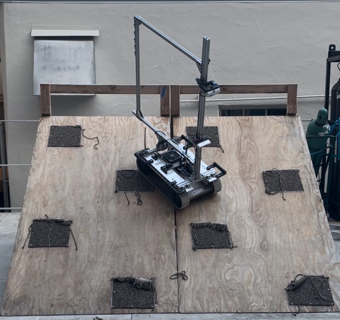
Figure 4: An image of the physical mobile robot platform on the inclined surface during a validation experiment. The carpet patches on the slope cause higher friction coefficients, resulting in slip uncertainty when only one of the tracks is on a patch.

We used CBF (76) with ${\tau=1.0~{}[m]}$, ${\xi_{\theta}=0.1}$ and the desired controller ${\mathbf{k_{d}}}$:

$$\mathbf{k_{d}}(x)=\begin{bmatrix}K_{v}\left\|\begin{bmatrix}x_{g}-x^{I}\\ y_{g}-y^{I}\end{bmatrix}\right\|\\[11.38109pt] K_{\omega}\dfrac{y_{g}-y^{I}}{\left\|\begin{bmatrix}x_{g}-x^{I}\\ y_{g}-y^{I}\end{bmatrix}\right\|}-K_{\omega}\sin{\theta}\end{bmatrix},$$

where ${x_{g},~{}y_{g}}$ are the goal position of the robot in the ${x^{I},y^{I}}$ directions, and ${K_{v},~{}K_{\omega}}$ are the controller gains. The control input set of the robot is given by:

$$U\triangleq\left\{u\in\mathbb{R}^{2}:\begin{bmatrix}-v_{\rm max}\\ -\omega_{\rm max}\end{bmatrix}\leq u\leq\begin{bmatrix}v_{\rm max}\\ \omega_{\rm max}\end{bmatrix}\right\}.$$

The parameters of the hardware experiments using the proposed safety-critical control method are given in Table 2. The control loops were realized at 50 Hz loop rate.

$K_{v}=1$	$x_{g}=1~{}[m],\ y_{g}=1.5~{}[m]$
$K_{\omega}=1.2$	$x(0)=[0~{}0~{}0]^{T}$
$\alpha_{h}=1,~{}\sigma_{V}=1$	$v_{\rm max}=0.5~{}[{m/s}]$
$H=\operatorname{diag}(8,8,8)$	$\omega_{\rm max}=0.5~{}[{rad/s}]$
$\Lambda=\operatorname{diag}(4,4,4)$	$\delta_{L}=0.5,~{}~{}\delta_{b}=1.5$

Table 2: Parameters of the mobile robot experiment.

The reference trajectory of the robot is chosen to yield a violation of the safety constraint when using the desired controller. The robot trajectory using a CBF-QP approach leaves the safe set due to the unmodelled uncertainty, as seen in Fig. 5 (Right) (Middle) and (Bottom). Note that the uncertainty vector is the difference between the discrete-time derivative of the flow map of the experimental system and the nominal robot model. The closed-loop safe behavior of the system under the proposed control method is shown in the same figures. As seen in the figures, under the proposed method, the states of the robot stay within the 0-superlevel set of the chosen CBF. Fig. 5 (Center) demonstrates that the proposed approach can estimate the model uncertainty, which affects the safety constraints.

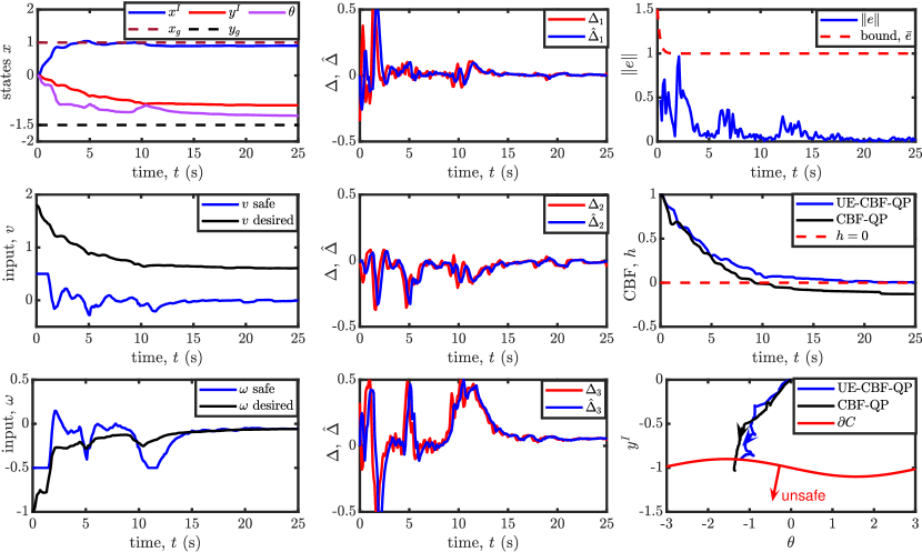
Figure 5: Experimental results for the mobile robot example of Fig. 4. (Left) (Top) The state trajectories (${x^{I}~{}[m],~{}y^{I}~{}[m],~{}\theta~{}[rad]}$) with the goal position of the robot operating under the UE-CBF-QP. (Middle) and (Bottom) The values of the safe linear velocity input, $v~{}[m/s]$ safe, the angular velocity input, $\omega~{}[rad/s]$ safe, and the desired control inputs, $v$ desired, $\omega$ desired, vs. time, respectively. (Center) The uncertainty estimator tracks the actual modelling inaccuracies. The first and last components of the uncertainty vector are ${\Delta_{1}}$ and ${\Delta_{3}}$, respectively. (Right) (Top) The uncertainty estimation error stays within the derived theoretical bounds. The value of CBF $h$ vs. time and trajectory of the system with the boundary of the safe set (Middle) and (Bottom). The proposed UE-CBF-QP-based safety filter maintains a safe distance from an edge on a slope in the presence of unmodelled dynamics. However, the robot under CBF-QP controller leaves the safe set due to the slope-induced uncertainty.

9 Conclusions and Future Work

This paper presented a method to synthesize robust controllers with formal safety guarantees for nonlinear systems in the presence of unmatched uncertainty. A novel uncertainty estimator is established for the state and input-dependent uncertainty, leading to bound in the framework of CBFs. By incorporating the estimator with CBFs and HOCBFs, robust safety conditions were derived. The effectiveness of the proposed robust safe control frameworks was experimentally demonstrated by controlling a tracked mobile robot on a slope while relying on a reduced-order nominal model.

Future work involves eliminating the knowledge of the bound $\delta_{L}$ by using data-driven techniques. Additionally, the proposed method can also consider state estimation errors.

References

[]Ersin Daş (Member, IEEE) is a postdoctoral researcher at Caltech. He received his B.S. degree in Mechatronics Engineering from Kocaeli University and his MSc degree in Mechatronics Engineering from Istanbul Technical University. He completed his PhD in mechanical engineering at Hacettepe University. His research interests lie at the intersection of robotics, safety-critical control, robust control, data-driven control, system identification, and machine learning.

[]Joel W. Burdick (Member, IEEE) is a Hayman Professor at Caltech, and a Jet Propulsion Laboratory Research Scientist. He focuses on robotics, kinematics, mechanical systems and control. Active research areas include: robotic locomotion, sensor-based motion planning algorithms, multi-fingered robotic manipulation, applied nonlinear control theory, neural prosthetics, and medical applications of robotics. He received his B.S. from Duke University and his Ph.D. from Stanford University.

References

• [1] J. Guiochet, M. Machin, and H. Waeselynck, “Safety-critical advanced robots: A survey,” Robotics and Autonomous Systems, vol. 94, pp. 43–52, 2017.
• [2] A. D. Ames, X. Xu, J. W. Grizzle, and P. Tabuada, “Control barrier function based quadratic programs for safety critical systems,” Transactions on Automatic Control, vol. 62, no. 8, pp. 3861–3876, 2017.
• [3] K. P. Wabersich, A. J. Taylor, J. J. Choi, K. Sreenath, C. J. Tomlin, A. D. Ames, and M. N. Zeilinger, “Data-driven safety filters: Hamilton-jacobi reachability, control barrier functions, and predictive methods for uncertain systems,” IEEE Control Systems Magazine, vol. 43, no. 5, pp. 137–177, 2023.
• [4] A. D. Ames, S. Coogan, M. Egerstedt, G. Notomista, K. Sreenath, and P. Tabuada, “Control barrier functions: Theory and applications,” in European Control Conf., 2019, pp. 3420–3431.
• [5] K.-C. Hsu, H. Hu, and J. F. Fisac, “The safety filter: A unified view of safety-critical control in autonomous systems,” arXiv preprint arXiv:2309.05837, 2023.
• [6] K. L. Hobbs, M. L. Mote, M. C. Abate, S. D. Coogan, and E. M. Feron, “Runtime assurance for safety-critical systems: An introduction to safety filtering approaches for complex control systems,” IEEE Control Systems Magazine, vol. 43, no. 2, pp. 28–65, 2023.
• [7] A. Alan, A. J. Taylor, C. R. He, A. D. Ames, and G. Orosz, “Control barrier functions and input-to-state safety with application to automated vehicles,” IEEE Trans. Control Systems Tech., 2023.
• [8] A. Singletary, A. Swann, Y. Chen, and A. D. Ames, “Onboard safety guarantees for racing drones: High-speed geofencing with control barrier functions,” IEEE Robotics and Automation Letters, vol. 7, no. 2, pp. 2897–2904, 2022.
• [9] R. Grandia, A. J. Taylor, A. D. Ames, and M. Hutter, “Multi-layered safety for legged robots via control barrier functions and model predictive control,” in 2021 IEEE International Conference on Robotics and Automation (ICRA).   IEEE, 2021, pp. 8352–8358.
• [10] A. Agrawal and K. Sreenath, “Discrete control barrier functions for safety-critical control of discrete systems with application to bipedal robot navigation.” in Robotics: Science and Systems, vol. 13.   Cambridge, MA, USA, 2017, pp. 1–10.
• [11] F. Ferraguti, C. T. Landi, S. Costi, M. Bonfè, S. Farsoni, C. Secchi, and C. Fantuzzi, “Safety barrier functions and multi-camera tracking for human–robot shared environment,” Robotics and Autonomous Systems, vol. 124, p. 103388, 2020.
• [12] X. Xu, P. Tabuada, J. W. Grizzle, and A. D. Ames, “Robustness of control barrier functions for safety critical control,” IFAC-PapersOnLine, vol. 48, no. 27, pp. 54–61, 2015.
• [13] A. Alan, T. G. Molnar, A. D. Ames, and G. Orosz, “Parameterized barrier functions to guarantee safety under uncertainty,” IEEE Control Systems Letters, 2023.
• [14] M. Jankovic, “Robust control barrier functions for constrained stabilization of nonlinear systems,” Automatica, vol. 96, pp. 359–367, 2018.
• [15] S. Kolathaya, J. Reher, A. Hereid, and A. D. Ames, “Input to state stabilizing control Lyapunov functions for robust bipedal robotic locomotion,” in 2018 Annual American Control Conference (ACC).   IEEE, 2018, pp. 2224–2230.
• [16] Q. Nguyen and K. Sreenath, “Robust safety-critical control for dynamic robotics,” IEEE Transactions on Automatic Control, 2021.
• [17] A. Alan, A. J. Taylor, C. R. He, G. Orosz, and A. D. Ames, “Safe controller synthesis with tunable input-to-state safe control barrier functions,” IEEE Control Systems Letters, 2021.
• [18] B. T. Lopez and J.-J. E. Slotine, “Unmatched control barrier functions: Certainty equivalence adaptive safety,” in 2023 American Control Conference (ACC).   IEEE, 2023, pp. 3662–3668.
• [19] A. J. Taylor and A. D. Ames, “Adaptive safety with control barrier functions,” in American Control Conference, 2020, pp. 1399–1405.
• [20] B. T. Lopez, J.-J. E. Slotine, and J. P. How, “Robust adaptive control barrier functions: An adaptive and data-driven approach to safety,” IEEE Control Systems Letters, vol. 5, no. 3, pp. 1031–1036, 2020.
• [21] M. Black, E. Arabi, and D. Panagou, “A fixed-time stable adaptation law for safety-critical control under parametric uncertainty,” in European Control Conf., 2021, pp. 1328–1333.
• [22] M. H. Cohen, C. Belta, and R. Tron, “Robust control barrier functions for nonlinear control systems with uncertainty: A duality-based approach,” in Conf. Decision and Control, 2022, pp. 174–179.
• [23] M. Cohen and C. Belta, Adaptive and Learning-Based Control of Safety-Critical Systems.   Springer Nature, 2023.
• [24] W.-H. Chen, J. Yang, L. Guo, and S. Li, “Disturbance-observer-based control and related methods—an overview,” IEEE Transactions on industrial electronics, vol. 63, no. 2, pp. 1083–1095, 2015.
• [25] B. Kürkçü, C. Kasnakoğlu, M. Ö. Efe, and R. Su, “On the existence of equivalent-input-disturbance and multiple integral augmentation via H-infinity synthesis for unmatched systems,” ISA transactions, vol. 131, pp. 299–310, 2022.
• [26] P. Zhao, Y. Mao, C. Tao, N. Hovakimyan, and X. Wang, “Adaptive robust quadratic programs using control lyapunov and barrier functions,” in IEEE Conf. Decision and Control.   IEEE, 2020, pp. 3353–3358.
• [27] E. Daş and R. M. Murray, “Robust safe control synthesis with disturbance observer-based control barrier functions,” in IEEE Conf. Decision and Control.   IEEE, 2022, pp. 5566–5573.
• [28] A. Alan, T. G. Molnar, E. Das, A. D. Ames, and G. Orosz, “Disturbance observers for robust safety-critical control with control barrier functions,” arXiv preprint arXiv:2209.08123, 2022.
• [29] Y. Wang and X. Xu, “Disturbance observer-based robust control barrier functions,” in 2023 American Control Conference (ACC).   IEEE, 2023, pp. 3681–3687.
• [30] Y. Cheng, P. Zhao, and N. Hovakimyan, “Safe model-free reinforcement learning using disturbance-observer-based control barrier functions,” arXiv preprint arXiv:2211.17250, 2022.
• [31] Q. Nguyen and K. Sreenath, “Exponential control barrier functions for enforcing high relative-degree safety-critical constraints,” in 2016 American Control Conference (ACC).   IEEE, 2016, pp. 322–328.
• [32] W. Xiao and C. Belta, “Control barrier functions for systems with high relative degree,” in IEEE Conf. Decision Control, 2019, pp. 474–479.
• [33] X. Tan, W. S. Cortez, and D. V. Dimarogonas, “High-order barrier functions: Robustness, safety, and performance-critical control,” IEEE Trans. Automatic Control, vol. 67, no. 6, pp. 3021–3028, 2021.
• [34] W. Xiao and C. Belta, “High-order control barrier functions,” IEEE Trans. Automatic Control, vol. 67, no. 7, pp. 3655–3662, 2021.
• [35] R. Takano and M. Yamakita, “Robust control barrier function for systems affected by a class of mismatched disturbances,” SICE J. Control, Meas., and Sys. Integ., vol. 13, no. 4, pp. 165–172, 2020.
• [36] A. Stotsky and I. Kolmanovsky, “Application of input estimation techniques to charge estimation and control in automotive engines,” Control Engineering Practice, vol. 10, no. 12, pp. 1371–1383, 2002.
• [37] H. Xie, L. Dai, Y. Lu, and Y. Xia, “Disturbance rejection MPC framework for input-affine nonlinear systems,” IEEE Transactions on Automatic Control, vol. 67, no. 12, pp. 6595–6610, 2021.
• [38] R. Sinha, J. Harrison, S. M. Richards, and M. Pavone, “Adaptive robust model predictive control with matched and unmatched uncertainty,” in 2022 American Control Conference (ACC).   IEEE, 2022, pp. 906–913.
• [39] A. Taylor, A. Singletary, Y. Yue, and A. Ames, “Learning for safety-critical control with control barrier functions,” in Learning for Dynamics and Control.   PMLR, 2020, pp. 708–717.
• [40] F. Castaneda, J. J. Choi, W. Jung, B. Zhang, C. J. Tomlin, and K. Sreenath, “Probabilistic safe online learning with control barrier functions,” arXiv preprint arXiv:2208.10733, 2022.
• [41] Y. Yang, H. Xu, and X. Yao, “Disturbance rejection event-triggered robust model predictive control for tracking of constrained uncertain robotic manipulators,” IEEE Transactions on Cybernetics, 2023.
• [42] Y. Yan, X.-F. Wang, B. J. Marshall, C. Liu, J. Yang, and W.-H. Chen, “Surviving disturbances: A predictive control framework with guaranteed safety,” Automatica, vol. 158, p. 111238, 2023.
• [43] J. Du, X. Hu, M. Krstić, and Y. Sun, “Robust dynamic positioning of ships with disturbances under input saturation,” Automatica, vol. 73, pp. 207–214, 2016.
• [44] S. Sastry, Nonlinear systems: analysis, stability, and control.   Springer Science & Business Media, 2013, vol. 10.
• [45] J. Yang, S. Li, and W.-H. Chen, “Nonlinear disturbance observer-based control for multi-input multi-output nonlinear systems subject to mismatching condition,” International Journal of Control, vol. 85, no. 8, pp. 1071–1082, 2012.
• [46] T. Posielek, K. Wulff, and J. Reger, “Analysis of sliding-mode control systems with relative degree altering perturbations,” Automatica, vol. 148, p. 110745, 2023.
• [47] E. D. Sontag and Y. Wang, “On characterizations of the input-to-state stability property,” Systems & Control Letters, vol. 24, no. 5, pp. 351–359, 1995.
• [48] A. Al Sawoor and M. Sadkane, “Lyapunov-based stability of delayed linear differential algebraic systems,” Applied Mathematics Letters, vol. 118, p. 107185, 2021.
• [49] T. Zou, J. Angeles, and F. Hassani, “Dynamic modeling and trajectory tracking control of unmanned tracked vehicles,” Robotics and Autonomous Systems, vol. 110, pp. 102–111, 2018.
• [50] M. Gianni, F. Ferri, M. Menna, and F. Pirri, “Adaptive robust three-dimensional trajectory tracking for actively articulated tracked vehicles,” Journal of Field Robotics, vol. 33, no. 7, pp. 901–930, 2016.
• [51] D. Wang and C. B. Low, “Modeling and analysis of skidding and slipping in wheeled mobile robots: Control design perspective,” IEEE Transactions on Robotics, vol. 24, no. 3, pp. 676–687, 2008.
• [52] M. S. Lobo, L. Vandenberghe, S. Boyd, and H. Lebret, “Applications of second-order cone programming,” Linear algebra and its applications, vol. 284, no. 1-3, pp. 193–228, 1998.
• [53] S. Dean, A. Taylor, R. Cosner, B. Recht, and A. Ames, “Guaranteeing safety of learned perception modules via measurement-robust control barrier functions,” in Conference on Robot Learning.   PMLR, 2021, pp. 654–670.
• [54] K. Long, V. Dhiman, M. Leok, J. Cortés, and N. Atanasov, “Safe control synthesis with uncertain dynamics and constraints,” IEEE Robotics and Automation Letters, vol. 7, no. 3, pp. 7295–7302, 2022.
• [55] J. Buch, S.-C. Liao, and P. Seiler, “Robust control barrier functions with sector-bounded uncertainties,” IEEE Control Systems Letters, vol. 6, pp. 1994–1999, 2021.
• [56] J.-J. E. Slotine, W. Li et al., Applied nonlinear control.   Prentice hall Englewood Cliffs, NJ, 1991, vol. 199, no. 1.
• [57] N. C. Janwani, E. Daş, T. Touma, S. X. Wei, T. G. Molnar, and J. W. Burdick, “A learning-based framework for safe human-robot collaboration with multiple backup control barrier functions,” arXiv preprint arXiv:2310.05865, 2023.
{IEEEbiography}