Multiple Imputation of Hierarchical Nonlinear Time Series Data with an Application to School Enrollment Data

Abstract

International comparisons of hierarchical time series data sets based on survey data, such as annual country-level estimates of school enrollment rates, can suffer from large amounts of missing data due to differing coverage of surveys across countries and across times. A popular approach to handling missing data in these settings is through multiple imputation, which can be especially effective when there is an auxiliary variable that is strongly predictive of and has a smaller amount of missing data than the variable of interest. However, standard methods for multiple imputation of hierarchical time series data can perform poorly when the auxiliary variable and the variable of interest are have a nonlinear relationship. Performance of standard multiple imputation methods can also suffer if the substantive analysis model of interest is uncongenial to the imputation model, which can be a common occurrence for social science data if the imputation phase is conducted independently of the analysis phase. We propose a Bayesian method for multiple imputation of hierarchical nonlinear time series data that uses a sequential decomposition of the joint distribution and incorporates smoothing splines to account for nonlinear relationships between variables. We compare the proposed method with existing multiple imputation methods through a simulation study and an application to secondary school enrollment data. We find that the proposed method can lead to substantial performance increases for estimation of parameters in uncongenial analysis models and for prediction of individual missing values.

1 Introduction

Missing values within hierarchical time series data sets are a common occurrence in social science data, particularly for comparisons across countries and across times that rely on survey data. International surveys may only be conducted in selected years and coverage of countries may differ from year to year, while country-level surveys and censuses may be conducted annually in some countries but may only occur sporadically in others. The presence of missing data can be compounded in settings that require the compilation of data from multiple different sources. One example where this occurs is for school enrollment data, where the UNESCO Institute for Statistics compiles survey and administrative data to create annual, internationally comparable estimates of school enrollment rates. The differing availability of survey and administrative data for each country and year leads to a large number of country-years in the UNESCO database where enrollment data is missing. Researchers interested in questions comparing survey-based indicators like enrollment rates across countries and across times can thus encounter large amounts of missing hierarchical time series data.

For some hierarchical time series variables, there may be related variables that that measure similar underlying concepts but have different amounts of missing data. For example, this can occur if a survey is designed to first ask for more specific information, but, failing to obtain the specific information, then asks for more general information. If the variable of interest for analysis is the variable that has a greater amount of missing data, researchers might be interested in how to best leverage the information from the auxiliary variable that has less missing data to impute the variable of interest. This situation arises with school enrollment data, where two commonly reported measures of enrollment rates are the Net Enrollment Rate (NER) and the Gross Enrollment Ratio (GER). Measurement of NER requires knowledge of the number and age distribution for children who are enrolled, while measurement of GER only requires knowledge of the number of children enrolled. The comparative ease of measuring GER can result in more missing values for NER compared to GER. If researchers are more interested in analyses using NER, they may want to use the available information about the auxiliary variable GER to help impute missing values for NER using a multiple imputation procedure.

Multiple imputation, first developed by Rubin (1978, 1987), is a widely used approach for handling missing data. In multiple imputation, $M>1$ imputed values for missing observations are sampled from the posterior predictive distribution of the missing data given the observed data. The $M$ imputed values result in $M$ completed data sets, each of which consists of the observed data and one set of imputed values for the missing observations. The completed data sets can each be analyzed separately using complete data methods and the results of the analyses can be combined into one final, pooled result using combining rules from Rubin (1987) that account for both within-imputation variation and between-imputation variation.

For hierarchical data, multiple imputation approaches that do not explicitly account for the hierarchical structure of the data can lead to biased results in downstream analyses (Taljaard et al., 2008; Enders et al., 2016; Lüdtke et al., 2017). Many approaches specifically for multiple imputation of hierarchical time series data have been developed (e.g. Liu et al., 2000; He et al., 2011; Speidel et al., 2018; Enders et al., 2020; Grund et al., 2021; among others), with two of the most widely used approaches for social science data being Amelia II and multilevel extensions of Multiple Imputation by Chained Equations (MICE). Amelia, originally developed by King et al. (2001) and extended as Amelia II by Honaker and King (2010), is a multiple imputation method designed specifically for hierarchical time series data. Amelia is based on the joint modeling approach to multiple imputation, where imputed values are sampled from a joint distribution for all variables with missing data. MICE is a multiple imputation method developed by van Buuren and Groothuis-Oudshoorn (2011) that uses the fully conditional specification (FCS) approach to multiple imputation. Rather than explicitly specifying a joint imputation model, the FCS algorithm iteratively samples from univariate conditional imputation models for all variables with missing data until convergence is reached. Several methods that account for hierarchical data structures have been implemented within the MICE framework, including the linear mixed effects method developed by Schafer and Yucel (2002). These commonly used methods assume that variables in the imputation model have a linear relationship. In settings where variables have a strong nonlinear relationship and transformation to approximate linearity is not possible, these methods are misspecified and can result in poor imputations.

We focus on the setting where the imputation of missing values and the analysis of imputed values are conducted independently. The development of multiple imputation originated in this setting, where Rubin (1977, 1978) proposed the multiple imputation framework as a way to provide imputed values for missing responses in public-use releases of large data sets from sample surveys. An appealing feature of multiple imputation for practitioners is the ability to use the same imputed data set to conduct many different analyses (Schafer, 1997a; Rubin, 1987). However, using the same multiply imputed data for different analyses can lead to the analysis model being uncongenial to the imputation model in the sense of Meng (1994). The analysis model and the imputation model are congenial if the imputation model contains at least as much information as the analysis model. Many of the theoretical properties of multiply imputed estimates, such as the consistency of estimates using Rubin’s combining rules, rely on congeniality (Meng, 1994; Rubin, 1996; Xie and Meng, 2017). In practice, uncongeniality of the analysis and imputation models can be a regular occurrence when the researchers that collect the survey data create imputed values for publication that are then used in analyses by external researchers. The external researchers may not have access to the same information or resources needed to create imputations of their own, for example if the imputation process is not well-documented or if the predictive variables used in the imputation model are not publicly available. In this scenario, the analysis models used by the external researchers are not guaranteed to be congenial to the imputation model. The ability of a multiple imputation method to perform well for uncongenial analyses is thus of interest for practitioners.

In this paper, we propose a multiple imputation method for continuous hierarchical time series data that can account for nonlinear relationships between variables. We refer to this method as MINTS for Multiple Imputation of hierarchical Nonlinear Time Series data. We focus on the bivariate setting, where one variable is the variable of interest for which imputations are desired and the second variable is an auxiliary variable that is easier to measure and has a nonlinear relationship with the variable of interest. We also focus on a specific type of nonlinear relationship where the nonlinearity takes the form of a piecewise linear function. We evaluate the out-of-sample validation performance of MINTS using a simulation study that compares the performance of the proposed method with existing multiple imputation methods using simulated data, where we focus on estimating parameters in analysis models that are uncongenial to the imputation model. We also conduct two validation exercises using a motivating data set on secondary school enrollment rates, where we evaluate the predictive performance for estimating individual missing values and for estimating parameters in uncongenial analysis models. Finally, we report the imputation results using the full enrollment data and make available a data set including 40 multiple imputations for NER and GER.

This paper is structured as follows. In Section 2, we describe the motivating case study of secondary school enrollment data in further detail. Section 3 describes the proposed multiple imputation method. In Sections 4 and 5, we evaluate how well the proposed multiple imputation method performs for estimation of parameters in uncongenial analysis models and for prediction of individual missing observations through a simulation study and an application to the enrollment data. Section 6 includes further discussion and comparison to existing imputation methods. Finally, we summarize the findings of this paper in Section 7.

2 Motivating Case Study: Secondary School Enrollment Rates

The UNESCO Institute for Statistics collects internationally comparable data on education indicators on an annual basis for all countries of the world, based largely on survey and administrative data (UNESCO Institute for Statistics, 2023). The World Bank combines this education data with population data from the United Nations Population Division to create estimates of two types of enrollment rates: the Net Enrollment Rate (NER) and the Gross Enrollment Ratio (GER) (World Bank, 2021). We focus on secondary school enrollment. NER is the ratio of children of official secondary school age who are enrolled in secondary school to the population of official secondary school age children. NER is bounded between 0% and 100% and both the numerator and denominator reflect children of official secondary school age. GER is the ratio of total enrollment in secondary school, regardless of age, to the population of official secondary school age children. The numerator and denominator for GER potentially represent different populations, where children who are not of official secondary school age can be counted in the numerator but not in the denominator. Thus, GER can be greater than 100% if children who are enrolled in secondary school are not of official school age. The two measures of enrollment are subject to the boundary NER $\leq$ GER and have a strong nonlinear relationship that can be well-approximated by a piecewise linear function.

For substantive analyses, one measure of enrollment may be preferred over the other. NER can be thought of as a demographic rate, where the numerator counts the number of enrollments for the population of children of official secondary school age in a given year and the denominator counts the person-years lived in that population for the given year. NER can thus be preferable over GER for demographic analyses. However, historical time series of NER tend to have more missing values than time series of GER. Measurement of NER is more difficult than measurement of GER due to requiring knowledge of the age distribution for children enrolled in secondary school. Measurement of GER is comparatively easy, as GER can be calculated using only the number of children who are currently enrolled. For school systems that do not have robust recordkeeping systems and countries that do not have good vital registration systems, knowledge of the age of all enrolled children can be difficult to obtain. The greater availability of estimates of GER and the strong relationship between NER and GER motivates the desire to impute missing values of NER using the relationship between NER and GER.

We obtain estimates of secondary school enrollment rates for both genders combined from World Bank (2021), where the definition of secondary school used for each country is based on the International Standard Classification of Education. After excluding all countries and years in the World Bank data base with no observations for either NER or GER, the resulting data set includes 202 countries and 51 years spanning 1970 to 2020 for a total of 10,302 country-year combinations. The overall rate of missingness is about 73.0% for NER and about 37.6% for GER. Within countries, the rate of missingness for NER ranges from about 13.7% missing in Malta to 100% missing in 14 countries. For GER, the rate of missingness within countries ranges from about 2.0% missing in Peru to about 98.0% missing in Curaçao.

Figure 1 shows a scatter plot of the complete cases for NER and GER. The red line illustrates the B-spline of degree 1 fit to the complete cases using the A-splines methodology described in Section 3.2.5. There is a nonlinear relationship between NER and GER, with a shift in trend occurring around GER $=100$. The variation of NER about the fitted spline also appears to vary with GER, with smaller variability at the lowest levels of GER and larger variability around GER $=100$.

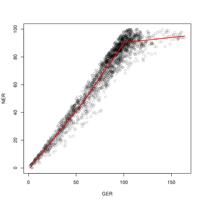
Figure 1: Scatter plot of complete cases for NER and GER from secondary enrollment data set, with the B-spline of degree 1 fit using A-splines superimposed in red.

Time series of NER and GER are shown in Figure 2 for Afghanistan, Belgium, Spain, and Nigeria. Afghanistan is an example of the most common type of pattern seen for individual countries, where there is a larger number of observed values for GER compared to NER. Only one country, Brazil, has the opposite pattern with one more observed value of GER than observed values of NER. Belgium and Spain are two examples of countries where the nonlinear relationship between NER and GER is visible in the time series for the individual country. Both Belgium and Spain have relatively few missing values for GER, but have large stretches of time with no observations for NER. Finally, Nigeria is an example of a country that has some observed values for GER but has no observed values for NER. There are 14 countries in the enrollment data set that, like Nigeria, have at least one observation for GER but no observations for NER.

Figure 2: Observed values of NER and GER for selected countries from secondary enrollment data set. Solid black and red circles indicate observed values for GER and NER, respectively.

3 Methods

3.1 Notation

We consider hierarchical time series data where the clustering variable is country and the time variable is year. Let $X_{c,t}$ denote the auxiliary variable and let $Y_{c,t}$ denote the variable of interest for country $c$ and year $t$, where $c\in 1,...,C$ and $t\in 1,...,T$. The vector of $X_{c,t}$ for all countries at year $t$ is denoted by $\mathbf{X}_{t}=\left[X_{1,t},X_{2,t},...,X_{C,t}\right]$. Similarly, the vector of $Y_{c,t}$ for all countries at year $t$ is denoted by $\mathbf{Y}_{t}=\left[Y_{1,t},Y_{2,t},...,Y_{C,t}\right]$. The $C$ by $T$ matrix of all $X_{c,t}$ is $\mathbf{X}=\left[\mathbf{X}_{1},\mathbf{X}_{2},...,\mathbf{X}_{T}\right]$ and the $C$ by $T$ matrix of all $Y_{c,t}$ is $\mathbf{Y}=\left[\mathbf{Y}_{1},\mathbf{Y}_{2},...,\mathbf{Y}_{T}\right]$.

Let the matrices $\mathbf{R}^{X}$ and $\mathbf{R}^{Y}$ denote the response matrices for $\mathbf{X}$ and $\mathbf{Y}$, respectively. If an element $(c,t)$ is observed, then the corresponding element of the response matrix equals 1. For example, if $X_{c,t}$ is observed, then $R_{c,t}^{X}=1$. If $X_{c,t}$ is missing, then $R_{c,t}^{X}=0$. The matrices $\mathbf{X}$ and $\mathbf{Y}$ can also be written in terms of their observed and missing portions, e.g. $\mathbf{X}=[\mathbf{X}_{mis},\mathbf{X}_{obs}]$ where the observed portion of $\mathbf{X}$ is denoted $\mathbf{X}_{obs}$ and the unobserved portion of $\mathbf{X}$ is denoted $\mathbf{X}_{mis}$.

For the enrollment data, the auxiliary variable $\mathbf{X}$ is GER and the variable of interest $\mathbf{Y}$ is NER. The enrollment data includes a total of $C=202$ countries, where the assignment of countries to indices $c\in 1,...,C$ was done alphabetically by country name. There are $T=51$ years in the enrollment data set, where $t=1$ corresponds to the year 1970 and $t=51$ corresponds to the year 2020.

3.2 Model

3.2.1 Assumptions

We assume the missing data mechanism is ignorable, i.e. the missing data mechanism is Missing At Random (MAR, defined in Section 4.3) and the parameters of the complete data model for ($\mathbf{X},\mathbf{Y}$) are distinct and a priori independent from the parameters of the missing data model governing the response matrices $\mathbf{R}^{X},\mathbf{R}^{Y}$ (Rubin, 1976; Schafer, 1997a; Little and Rubin, 2002). The assumption of ignorability allows for imputation without specification of a model for the missing data mechanism. Using $\mathbf{X}$ as an example, imputed values are said to be Bayesianly proper in the sense of Schafer (1997a) if they are independently drawn from the posterior distribution $p(\mathbf{X}_{mis}|\mathbf{X}_{obs},\mathbf{R}^{X})$. When the missing data mechanism is ignorable, proper imputations can instead be drawn from the posterior distribution $p(\mathbf{X}_{mis}|\mathbf{X}_{obs})=\int p(\mathbf{X}_{mis}|\mathbf{X}_{obs},\theta)p(\theta|\mathbf{X}_{obs})d\theta$ where $\theta$ is the vector of parameters for the complete data. The assumption of ignorability is ubiquitous for general-purpose imputation models, but in practice researchers cannot know if this assumption is met. We conducted sensitivity analyses in Sections 4 and 5 to evaluate how well the MINTS method performs when the ignorability assumption is violated.

Finally, we assume that the auxiliary variable is observed at least once for each country for which we are interested in imputing the variable of interest. That is, both $\mathbf{X}$ and $\mathbf{Y}$ can contain missing values for any country-year, but we assume that each country has at least one year in which $X_{c,t}$ is observed. This reflects the motivating setting for the proposed imputation method, where the auxiliary variable is more likely to be observed in each country than the variable of interest due to being easier to measure. This assumption is satisfied for the enrollment data, where after the exclusion of countries that have no observed values for either NER or GER, the remaining countries all have at least one observed value of GER.

3.2.2 Sequential Decomposition of Joint Model

The MINTS method uses a variation of the joint modeling approach to multiple imputation. In the usual joint modeling approach, the complete data $(\mathbf{X},\mathbf{Y})$ is assumed to follow a multivariate joint distribution and imputed values are sampled from the joint posterior predictive distribution of the missing data given the observed data. One downside to this approach is the difficulty of specifying a joint distribution for all variables used in the imputation model. A common general-purpose choice for the joint distribution is the multivariate normal distribution, which has been found to still perform reasonably for imputation even when the assumption of normality is violated (Schafer, 1997a; Schafer and Olsen, 1998). However, if there are nonlinear relationships between variables in the imputation model, joint modeling assuming multivariate normality is unable to incorporate those relationships.

A more flexible approach to multiple imputation is the fully conditional specification (FCS) approach, also known as imputation via chained equations (van Buuren et al., 2006) and sequential regression multivariate imputation (Raghunathan et al., 2001), among other names. FCS does not explicitly specify a joint distribution for the variables with missing data. Instead, univariate conditional distributions are specified for each variable with missing data given all the other variables in the imputation model. Missing values are imputed by iteratively sampling from the univariate conditional distributions until convergence for all imputation model parameters is reached. The conditional distributions can take any form and can accommodate nonlinear relationships between variables. However, this level of flexibility can lead to cases where the univariate conditional distributions are not compatible. Although simulation studies show that FCS can result in reasonable imputations even when the conditional distributions are not compatible (e.g. van Buuren et al., 2006), ultimately FCS does not guarantee that the iterative conditional algorithm will converge to a proper joint distribution.

We use an alternative to the usual joint modeling approach that combines desirable features of joint modeling and FCS through a sequential decomposition of the joint model. The sequential decomposition approach for joint modeling was first proposed by Lipsitz and Ibrahim (1996) and has been extended by Ibrahim et al. (1999, 2002); Lee and Mitra (2016); Xu et al. (2016); Lüdtke et al. (2020); among others. The joint distribution of the variables with missing data is decomposed into a sequence of univariate conditional distributions. One possible decomposition of the joint distribution for $(\mathbf{X},\mathbf{Y})$ is

$$p(\mathbf{X},\mathbf{Y}|\bm{\theta})= p(\mathbf{Y}|\mathbf{X},\bm{\theta}_{Y})p(\mathbf{X}|\bm{\theta}_{X}).$$ (1)

The vector of parameters for the joint distribution is $\bm{\theta}$, the vector of parameters for the conditional distribution of $\mathbf{Y}|\mathbf{X}$ is $\bm{\theta}_{Y}$, and the vector of parameters for the distribution of $\mathbf{X}$ is $\bm{\theta}_{X}$. Unlike in FCS, this sequence of univariate conditional distributions is guaranteed to correspond to a well-defined joint distribution by construction.

The sequential decomposition approach allows for greater flexibility compared to joint modeling, but is not quite as flexible as FCS due to the additional restriction of requiring an ordering for the conditional distributions. The choice of ordering can have a substantial impact on the performance of the imputation model due to the risk of conditional distributions being incorrectly specified. We follow standard guidelines proposed by Rubin and Schafer (1990) and choose the ordering based on the percentage of missing values. For the ordering in Equation 1, the variable of interest $\mathbf{Y}$ has a larger amount of missing data compared to the auxiliary variable $\mathbf{X}$.

3.2.3 Model Specification

The joint distribution of $(\mathbf{Y},\mathbf{X})$ is decomposed sequentially following Equation 1 as the product of the distribution of $\mathbf{Y}|\mathbf{X}$ and the distribution of $\mathbf{X}$. The distribution of $\mathbf{X}$ is further decomposed as

$$p(\mathbf{X}|\bm{\theta}_{X})= \Bigg{(}\prod_{t=1}^{T}p(\mathbf{X}_{t}|\mathbf{X}_{t-1},\bm{\theta}_{X})\Bigg{)}p(\mathbf{X}_{0}|\bm{\theta}_{X}),$$

where $\mathbf{X}_{0}$ is a parameter that represents the vector of $X_{c,0}$ for all countries $c$ at the unobserved year $t=0$. Similarly, the conditional distribution of $\mathbf{Y}|\mathbf{X}$ is further decomposed as

$$p(\mathbf{Y}|\mathbf{X},\bm{\theta}_{Y})= \left(\prod_{t=1}^{T}p(\mathbf{Y}_{t}|\mathbf{Y}_{t-1},\mathbf{X}_{t},\bm{\theta}_{Y})\right)p(\mathbf{Y}_{0}|\mathbf{X}_{0},\bm{\theta}_{Y}),$$

where $\mathbf{Y}_{0}$ is a parameter that represents the vector of $Y_{c,0}$ for all countries $c$ at the unobserved year $t=0$.

The distribution of $\mathbf{X}_{t}|\mathbf{X}_{t-1},\bm{\theta}_{X}$ is modeled as a random walk with a country-specific drift term $\gamma_{c}$. For country $c$ and $t\in 1,...,T$,

$$X_{c,t}|X_{c,t-1},\bm{\theta}_{X}\sim \,TN_{[X_{low},X_{up}]}(X_{c,t-1}+\gamma_{c},\,\sigma_{X}^{2}),$$ (2)

where $TN_{[X_{low},X_{up}]}$ refers to the truncated normal distribution with lower bound $X_{low}$ and upper bound $X_{up}$. These boundaries can vary with $(c,t)$, but the dependency is suppressed in the notation.

The conditional distribution of $\mathbf{Y}_{t}|\mathbf{Y}_{t-1},\mathbf{X}_{t},\bm{\theta}_{Y}$ is modeled with a country-specific intercept $\alpha_{c}$, a nonlinear function $f$ of $\mathbf{X}$ with coefficient $\beta$, and an AR(1) term with autoregressive parameter $\rho$. The variance model for $\mathbf{Y}_{t}|\mathbf{Y}_{t-1},\mathbf{X}_{t},\bm{\theta}_{Y}$ models heteroscedasticity as a function $h$ of $\mathbf{X}$. For country $c$ and $t\in 1,...,T$,

$$Y_{c,t}|Y_{c,t-1},X_{c,t},\bm{\theta}_{Y}\sim \,TN_{[Y_{low},Y_{up}]}\left(\alpha_{c}+\beta\,f(X_{c,t})+\rho\,Y_{c,t-1},\,\sigma_{Y}^{2}\,h(X_{c,t})\right),$$ (3)

where $TN_{[Y_{low},Y_{up}]}$ refers to the truncated normal distribution with lower bound $Y_{low}$ and upper bound $Y_{up}$. These boundaries can vary with $(c,t)$, but the dependency is suppressed in the notation.

3.2.4 Prior Distributions

The prior distributions are specified as

$$\sigma_{X}^{2}\sim InvGamma(2,\delta_{X}),$$

$$\gamma_{c}\sim N(\mu_{drift},\sigma_{drift}^{2}),$$

$$\mu_{drift}\sim N(\nu_{drift},\zeta_{drift}^{2}),$$

$$\sigma_{drift^{2}}\sim InvGamma(2,\delta_{drift}),$$

$$\sigma_{Y}^{2}\sim InvGamma(2,\delta_{Y}),$$

$$\alpha_{c}\sim N(\mu_{0},\sigma_{0}^{2}),$$

$$\mu_{0}\sim N(0,\zeta_{0}^{2}),$$

$$\sigma_{0}^{2}\sim InvGamma(2,\delta_{0}),$$

$$\beta\sim N(0,1),$$

$$\rho\sim U(0,1),$$

where the hyperparameters $\delta_{X},\nu_{drift},\zeta_{drift},\delta_{drift},\delta_{Y},\zeta_{0},\text{and }\delta_{0}$ are control parameters that are used to adjust the prior distributions to the appropriate scale for the data.

For all $c$, the joint prior distribution of $(Y_{c,0},X_{c,0})$ is a truncated normal distribution with control parameters $\bm{\mu}_{early}$ and $\bm{\Sigma}_{early}$ given by

$$\left[\begin{matrix}Y_{c,0}\\ X_{c,0}\end{matrix}\right]\sim \,TN\left(\bm{\mu}_{early},\bm{\Sigma}_{early}\right).$$

The truncation is such that $X_{c,0}\in[X_{0,low},X_{0,up}]$ and $Y_{c,0}\in[Y_{0,low},Y_{0,up}]$ where the boundaries can vary with $c$ but this dependency is suppressed in the notation. The control parameters $\bm{\mu}_{early}$ and $\bm{\Sigma}_{early}$ are shared across all $c$.

Priors were chosen to be conjugate and diffuse for most parameters. An informative prior was used for the autoregressive parameter $\rho$ in the imputation model for $\mathbf{Y}|\mathbf{X}$ to reflect the prior belief that $\mathbf{Y}$ is generally increasing over time for the motivating enrollment data, but should generally be specified based on the data being imputed. The values for all hyperparameters should ideally be determined using prior expert knowledge. However, in missing data problems where a general-purpose imputation method is used, the imputer generally does not possess such knowledge for the choice of hyperparameters. In the absence of expert information, we instead propose an algorithm for specifying diffuse priors dictated by data-based control parameters, details of which are in the Appendix. The prior distributions were chosen to be sufficiently diffuse such that the data-based control parameters do not overwhelm the posterior inference following the philosophy of Edwards et al. (1963). We note that use of the data-based algorithm to specify prior distributions results in an approximate posterior distribution rather than a fully Bayesian posterior distribution.

3.2.5 A-splines

The nonlinear functions $f$ and $h$ in Equation 3 are estimated through spline regression using the complete cases in $(\mathbf{X},\mathbf{Y})$. To estimate $f$, the model $Y_{c,t}=f(X_{c,t})+\varepsilon^{f}_{c,t}$ is fit with Gaussian errors using a B-spline of degree 1. The residuals from the estimation of $f$ are then used to estimate $h$ by fitting the model $|Y_{c,t}-f(X_{c,t})|=h(X_{c,t})+\varepsilon^{h}_{c,t}$ with Gaussian errors and using a B-spline of degree 1. After estimation, $f$ is truncated to have range $[Y_{low},Y_{up}]$ and $h$ is truncated to have range $[\epsilon,\infty)$, where $\epsilon$ is a small positive value. The number and placement of knots for the B-splines used for $f$ and $h$ are selected using a method called adaptive splines, or A-splines (Goepp et al., 2018). A-splines automates the selection of knots using an iterative penalized likelihood approach and is implemented in the R package “aspline” (Goepp, 2022).

3.3 Estimation

3.3.1 Model Estimation

The MINTS model is estimated using a Markov chain Monte Carlo (MCMC) algorithm with Gibbs sampling and Metropolis-Hastings steps in R. Multiple imputations are created in two phases. The parameters of the imputation model are first estimated in the estimation phase. In the imputation phase, additional iterations from the same MCMC algorithm are run and used to create multiply imputed data sets.

Estimation of the imputation model parameters occurs simultaneously with estimation of the missing values in a similar fashion to the data augmentation algorithm of Tanner and Wong (1987), with the MCMC algorithm resulting in samples from the joint posterior distribution of the imputation model parameters and the missing values given the observed data. At each iteration of the MCMC algorithm, two steps are iterated until convergence is reached. First, values of the imputation model parameters are drawn from their posterior distributions given the observed data and the most recent estimates of the missing values. Second, estimates for the missing values are drawn from their posterior distributions given the observed data and the previously drawn imputation model parameters. Let $\bm{\theta}_{X}=(\bm{\gamma},\sigma_{X}^{2},\mathbf{X}_{0},\mu_{drift},\sigma^{2}_{drift})$ and $\bm{\theta}_{Y}=(\bm{\alpha},\beta,\rho,\sigma_{Y}^{2},\mathbf{Y}_{0},\mu_{0},\sigma^{2}_{0})$ denote the parameters of the models for $\mathbf{X}$ and $\mathbf{Y}|\mathbf{X}$, respectively. The general approach of the MCMC algorithm proceeds as follows for iterations $i=1,...,n_{iter}$:

1. Draw $\bm{\theta}_{X}^{(i)}$ from $p(\bm{\theta}_{X}|\mathbf{X}_{obs},\mathbf{X}_{mis}^{(i-1)})$

2. Let $j=1,...,J$ index the $X_{c,t}$ in $\mathbf{X}_{mis}$. For each $j$, draw $X^{(i)}_{j}$ from

   $$p(X_{j}|\mathbf{X}_{obs},X_{1}^{(i)},X_{2}^{(i)},...,X_{j-1}^{(i)},X_{j+1}^{(i-1)},...,X_{J}^{(i-1)},\bm{\theta}_{X}^{(i)})$$

3. Draw $\bm{\theta}_{Y}^{(i)}$ from $p(\bm{\theta}_{Y}|\mathbf{Y}_{obs},\mathbf{Y}_{mis}^{(i-1)},\mathbf{X}_{obs},\mathbf{X}_{mis}^{(i)})$

4. Let $k=1,...,K$ index the $Y_{c,t}$ in $\mathbf{Y}_{mis}$. For each $k$, draw $Y^{(i)}_{k}$ from

   $$p(Y_{k}|\mathbf{Y}_{obs},Y_{1}^{(i)},Y_{2}^{(i)},...,Y_{k-1}^{(i)},Y_{k+1}^{(i-1)},...,Y_{K}^{(i-1)},\mathbf{X}_{obs},\mathbf{X}_{mis}^{(i)},\bm{\theta}_{Y}^{(i)})$$

The total number of iterations $n_{iter}$ used in the estimation phase is determined based on convergence diagnostics such as inspection of trace plots and evaluation of the diagnostics of Raftery and Lewis (1996) and Gelman and Rubin (1992). Complete details of the MCMC algorithm can be found in the Appendix.

3.3.2 Imputation Procedure

After the MCMC algorithm has converged for estimation of the imputation model parameters, the imputation phase begins. All iterations of the MCMC that were required for convergence are treated as burn-in during the imputation phase. Imputed values for $\mathbf{X}_{mis}$ and $\mathbf{Y}_{mis}$ are created by continuing the MCMC algorithm with additional thinning steps. Thinning of the MCMC chains is required during the imputation phase to ensure that the imputed data sets are approximately independent draws from the posterior predictive distribution of the missing data given the observed data under the model described in Section 3.2.3 and priors described in Section 3.2.4. The amount of thinning is chosen so that the autocorrelation of the imputed values is approximately zero.

The number of iterations used in the imputation phase depends on the desired number of multiply imputed data sets, the number of chains of the MCMC, and the number of iterations used for thinning. To obtain $M$ multiply imputed data sets from $C$ chains with $n_{thin}$ iterations between imputed values, the MCMC algorithm is run for an additional $\frac{M}{C}\times n_{thin}$ iterations for each chain.

4 Simulation Study

We conducted a simulation study to evaluate how well the MINTS method performs for estimation of analysis models that are uncongenial to the imputation model. We refer to this validation exercise as “analysis model validation.”

Analysis model validation was conducted for a simulated data set where a nonlinear relationship was simulated between variables. We considered nine experiments corresponding to three rates of simulated missingness and three missing data mechanisms. Each experiment was replicated $N_{rep}=1000$ times and the average performance across replications for MINTS was compared with the performance of existing multiple imputation methods for hierarchical time series data. Details of the simulation study using the nonlinear simulated data are presented in this section, while details of an analogous simulation study using linear simulated data are available in the Appendix.

4.1 Data Generation

Variables $\mathbf{X}$ and $\mathbf{Y}$ were generated for 20 countries and 30 years for a total sample size of 600 country-years. $\mathbf{Y}$ is the variable of interest for substantive analyses, while $\mathbf{X}$ is an auxiliary variable that is only of interest for imputation of $\mathbf{Y}$.

$\mathbf{X}$ was simulated independently for each country and is bounded in $[0,100]$. For country $c$,

$$X_{c,1}\sim \,U(X_{1,low},X_{1,up}),$$

$$X_{c,t+1}\sim \,TN_{[0,100]}(X_{c,t}+\gamma_{c},\sigma^{2})\text{ for $t=1,...,29$},$$

where $TN_{[0,100]}$ refers to the truncated normal distribution with support $[0,100]$ and $\gamma_{c}$ is a country-specific drift term. For the nonlinear simulated data, we set $X_{1,low}=0$, $X_{1,up}=25$, $\sigma^{2}=1$, and $\gamma_{c}\sim U(1,3)$.

$\mathbf{Y}$ was simulated to have a nonlinear relationship with $\mathbf{X}$ and is bounded as $Y_{c,t}\in[0,min(X_{c,t},60)]$. For country $c$,

$$Y_{c,t}\sim \,TN_{[0,\text{min}(X_{c,t},60)]}\Bigg{(}\alpha_{c}+\frac{40}{\big{(}1+\exp\big{(}-\frac{X_{c,t}-60}{8}\big{)}\big{)}}+3\log(X_{c,t}),1^{2}\Bigg{)},$$

$$\alpha_{c}\sim \,U(0,5),$$

where $TN_{[0,\text{min}(X_{c,t},60)]}$ refers to the truncated normal distribution with support $[0,\text{min}(X_{c,t},60)]$. $\mathbf{X}$ and $\mathbf{Y}$ were constructed to have a generally monotonically increasing relationship similar to the relationship observed for the enrollment data.

4.2 Analysis Model

We focused on the setting where the analysis model is uncongenial to the imputation model. The variable $\mathbf{Z}$ is treated as the outcome variable and was simulated to have a linear relationship with $\mathbf{Y}$. For each country $c$ and year $t$,

$$Z_{c,t}\sim \,N(\eta_{c}+2Y_{c,t},10^{2}),$$

$$\eta_{c}\sim \,U(0,15).$$

The analysis model is the linear regression of $\mathbf{Z}$ on $\mathbf{Y}$. The parameter of interest is $\omega_{1}$, the coefficient on $\mathbf{Y}$ in the regression

$$Z_{c,t}= \,\omega_{0}+\omega_{1}Y_{c,t}+\varepsilon_{c,t}^{\omega},$$

$$\varepsilon_{c,t}^{\omega}\sim N(0,\sigma_{\varepsilon_{\omega}}^{2}).$$

Additional validation results for a random intercept analysis model can be found in the Appendix.

4.3 Analysis Model Validation Procedure

Data was simulated as missing following the three missing data mechanisms of Rubin (1976): Missing Completely At Random (MCAR), Missing At Random (MAR), and Missing Not at Random (MNAR). For variable $\mathbf{X}$, MCAR occurs when $P(\mathbf{R}^{X}|\mathbf{X})=P(\mathbf{R}^{X})$. Data was simulated as missing under MCAR by assuming that each observation has the same probability of being missing. MAR occurs when $P(\mathbf{R}^{X}|\mathbf{X})=P(\mathbf{R}^{X}|\mathbf{X}_{obs})$. Data was simulated as missing under MAR by assuming that observations in earlier years are more likely to be missing. Finally, MNAR occurs when the probability of being missing depends on both the missing and the observed data and $P(\mathbf{R}^{X}|\mathbf{X})$ cannot be simplified further. Data was simulated as missing under MNAR by assuming that the probability of being missing depends on the observed values. All methods compared in the simulation study assume that the missing data mechanism is at least MAR, so the simulations using MNAR act as a sensitivity analysis. Details of the MAR and MNAR implementations can be found in the Appendix.

For each missing data mechanism, data was simulated as missing at the 10%, 40%, and 80% rates. Each combination of missing data mechanism and rate was implemented simultaneously for $\mathbf{X}$ and $\mathbf{Y}$ and defines an experiment. For example, the MCAR 10% experiment corresponds to the setting where 10% of $\mathbf{X}$ was simulated as missing under MCAR and 10% of $\mathbf{Y}$ was simulated as missing under MCAR. We note that while 80% is a high rate of missingness, it is similar to the observed rate of missingness for NER in the enrollment data set.

For each experiment, the analysis model validation procedure is

1. For replication $r=1,...,N_{rep}$,

   1. Simulate missing values according to the experiment’s missing data mechanism and rate to separate the data into “observed” and “missing” data

   2. Run the multiple imputation procedure using the observed data to create $M=40$ completed data sets. Completed data sets consist of the observed data and the imputed values for the missing data.

   3. Estimate quantities of interest $Q$ using each of the $M$ completed data sets

   4. Pool the estimates of $Q$ and $SE(Q)$ across the $M$ completed data sets using combining rules from Rubin (1987) to obtain the pooled estimates $\bar{Q}_{r}$ and $SE(\bar{Q}_{r})$

2. Calculate the true value of $Q$ using the full data set

3. Calculate evaluation metrics for the pooled estimates $\bar{Q}_{r}$ averaged across replications

The number of imputations $M=40$ was chosen to balance between having a large enough number of imputations to guarantee minimal contribution of simulation error to the variability of estimands and having a small enough number of imputations to be computationally feasible.

Pooled estimates for each scalar quantity of interest $Q$ are created using combining rules from Rubin (1987) in Step 1(d) of the validation procedure. Let $\hat{Q}_{m}$ denote the point estimate of $Q$ from imputation $m$ and let $\hat{U}_{m}$ denote its associated variance. The pooled point estimate of $Q$ across all $M$ imputations is $\bar{Q}_{M}=\frac{1}{M}\sum_{m=1}^{M}\hat{Q}_{m}$. The pooled variance estimate of $\bar{Q}_{M}$ is $T_{M}=\bar{U}_{M}+\left(1+\frac{1}{M}\right)B_{M}$, where $\bar{U}_{M}=\frac{1}{M}\sum_{m=1}^{M}\hat{U}_{m}$ is the average within-imputation variance and $B_{M}=\frac{1}{M-1}\sum_{m=1}^{M}(\hat{Q}_{m}-\bar{Q}_{M})^{T}(\hat{Q}_{m}-\bar{Q}_{M})$ is the between-imputation variance. The 95% confidence interval for the pooled estimate $\bar{Q}_{M}$ is constructed using $\bar{Q}_{M}\pm t_{\nu}^{*}\sqrt{T_{M}}$, where $t_{\nu}^{*}$ is the critical value for 95% confidence from the $t$ distribution with $\nu$ degrees of freedom. The degrees of freedom $\nu$ for finite number of imputations $M$ is $\nu=(M-1)(1+\frac{1}{r_{M}})^{2}$, where $r_{M}$ is the relative increase in variance due to nonresponse given by $r_{M}=\left(1+\frac{1}{M}\right)\frac{B_{M}}{\bar{U}_{M}}$.

The performance of the point estimates $\bar{Q}_{M}$ was evaluated using the mean absolute error (MAE), calculated as $\frac{1}{N_{rep}}\sum_{r}|\bar{Q}_{M}-Q|$ where the sum is taken over all replications within each experiment. The performance of the 95% confidence intervals for the pooled estimates $\bar{Q}_{M}$ was evaluated by using the mean coverage across all replications within each experiment, calculated as the proportion of intervals that contained the true value. We also evaluated the mean fraction of Fisher information about $Q$ that is missing due to nonresponse, which we abbreviate as FMI for Fraction of Missing Information. In each replication of each experiment, FMI is estimated as

$$\text{FMI}= \frac{r_{M}+\frac{2}{\nu+3}}{r_{M}+1}.$$

The mean FMI across all replications within each experiment enables assessment of the amount of information about $Q$ that is lost due to the presence of missing data (Schafer, 1997a; Savalei and Rhemtulla, 2012). We note that with $M=40$ imputations, the estimates of FMI may be noisy, so in this case FMI should only be interpreted as an exploratory diagnostic (Bodner, 2008; Enders, 2010).

4.4 Model Implementation

For each replication of each experiment, we created 40 imputations using the MINTS method by running 10 chains of the MCMC algorithm. The bounds of the model for $\mathbf{X}$ were set as $X_{low}=0$ and $X_{up}=100$ and the bounds of the model for $\mathbf{Y}|\mathbf{X}$ were set as $Y_{low}=0$ and $Y_{up}=\text{min}(X_{c,t},60)$. During the estimation phase, the MCMC was run for enough iterations to ensure convergence of all imputation model parameters. The number of iterations differed across experiments, but ranged from 10000 to 25000 iterations per chain. During the imputation phase, an additional 4000 iterations was run for each chain and four iterations from each chain were selected as the imputed values. The iterations selected as the final imputed values were chosen to be 1000 iterations apart to ensure autocorrelation was close to zero following the procedure described in Section 3.3.2.

We compared the MINTS method to six models based on existing methods for multiple imputation. Three of these models are based on the MICE methodology as implemented in the R package “mice” (van Buuren and Groothuis-Oudshoorn, 2011). MICE uses the FCS algorithm, which allows for the specification of separate univariate conditional models for each variable with missing data. The univariate conditional models include all available variables as predictors, for example, the model for $\mathbf{X}$ includes $\mathbf{Y}$, year, and country as predictors. We first considered the default imputation method for continuous data in the mice package, which is predictive mean matching. We refer to this method as the MICE PMM method. Unlike the other methods considered, MICE PMM does not explicitly account for the hierarchical structure of the data but is included as a baseline for comparison.

We evaluated two models within the MICE framework that account for the hierarchical structure of the data using the method of Schafer (1997b) and Schafer and Yucel (2002), referred to as the pan method following its implementation in the R package “pan” (Zhao and Schafer, 2023). The function mice.impute.2l.pan within the mice package uses a Gibbs sampler to estimate the conditional linear mixed effects model with homogeneous within-group variances for each variable with missing data given the other variables. We evaluated a model that includes a country-specific intercept and fixed effects for all covariates in the imputation model, referred to as the pan Fixed Effects method. For example, imputed values for $X_{c,t}|Y_{c,t}$ are modeled with a country-specific intercept, a fixed effect of year, a fixed effect of $Y_{c,t}$, and a homogeneous normally distributed error term. We also considered the pan Random Effects method, which adds random effects of all covariates to the model used in the pan Fixed Effects method.

We evaluated three models using the Amelia II methodology as implemented in the R package “Amelia” (Honaker and King, 2010). For complete data $(\mathbf{X},\mathbf{Y})$, Amelia assumes the joint distribution is multivariate normal. The parameters of the joint distribution are estimated using a combination of bootstrapping and an EM algorithm. Amelia is designed specifically for imputation of hierarchical time series data, which Honaker and King refer to as time series cross-sectional data, through modeling features such as smooth trends over time and allowing for country-specific effects. For our comparisons, we evaluated three implementations of Amelia that were chosen to use the simplest form of the time-series-cross-sectional modeling features in Amelia: a time-series (TS) model, a cross-sectional (CS) model, and a time-series-cross-sectional (TSCS) model. All three of the imputation models are constructed by adding terms to the default multivariate normal joint model for $(\mathbf{X},\mathbf{Y})$. In the Amelia TS method, a linear effect of time is added. In the Amelia CS method, a country-specific intercept term is added. In the Amelia TSCS method, a country-specific intercept term and a country-specific linear effect of time are added.

Imputations were created using the default settings in mice and Amelia, with the exception of setting the number of imputations as $M=40$, specifying the form of the imputation models as described above, and specifying bounds of $\mathbf{X}\in[0,100]$ and $\mathbf{Y}\in[0,60]$. Scalar bounds were used for $\mathbf{Y}$ as the mice and Amelia packages do not allow for variable bounds.

4.5 Analysis Model Validation Results

For the linear regression analysis model validation, we evaluated how well each multiple imputation method performs for estimation of $Q=\omega_{1}$, the regression coefficient on $\mathbf{Y}$ in the linear regression of $\mathbf{Z}$ on $\mathbf{Y}$. Table 1 summarizes the results of this validation for the nonlinear simulated data. Overall, MINTS results in the best balance between MAE, coverage, and FMI across the nine experiments. MINTS has the smallest MAE in all experiments except MAR 10%, where MINTS has the second smallest MAE behind MICE PMM. At the 10% and 40% rates, MINTS has reasonably close to nominal coverage for 95% intervals. While MINTS has the closest to nominal coverage out of the methods compared in the experiments at the 80% rate, coverage is below nominal in all three experiments. MINTS also has the smallest FMI at the 10% and 40% rates. As expected, FMI is much larger for all methods at the 80% rate, with FMI $>50\%$ for several methods. This is higher than is typical for the setting of sample survey data that multiple imputation was originally designed for, where FMI is usually $\leq 30\%$ (Rubin, 2003). Given the high FMI, it is thus unsurprising how poorly all multiple imputation methods perform in the experiments at the 80% rate.

None of the existing methods perform consistently well across experiments for estimation of $\omega_{1}$. While MICE PMM can outperform the methods explicitly designed for hierarchical time series data at the lower rates of missingness, the performance of MICE PMM suffers greatly at the highest rate of missingness. The pan and Amelia methods perform similarly to one another at the 10% rate, but all have larger MAE than MICE PMM. Performance of the pan and Amelia methods generally is best under MCAR, with pan Random Effects and Amelia TSCS performing the best of the group in terms of MAE and coverage.

Table 1: Summary of analysis model validation for nonlinear simulated data for $Q=\omega_{1}$, the regression coefficient on $Y$ in the linear regression of $Z$ on $Y$. MAE denotes mean absolute error, Cvg denotes the average coverage of 95% intervals as a percentage, and FMI denotes the fraction of missing information as a percentage. MAE is multiplied by 100 before reporting. Results are averaged over the 1000 replications of each experiment. The true value of $Q$ is 2.060.

Simulated Method MCAR MAR MNAR Missingness Rate MAE Cvg FMI MAE Cvg FMI MAE Cvg FMI 10% MICE PMM 1.16 100.0 6.4 0.53 100.0 3.4 0.81 100.0 4.4 pan Fixed 1.78 100.0 6.0 6.34 93.3 7.1 3.43 100.0 5.5 pan Random 1.18 100.0 4.1 4.87 99.9 4.9 2.35 100.0 3.5 Amelia TS 1.87 100.0 7.1 5.64 99.8 7.6 3.37 100.0 6.0 Amelia CS 2.30 100.0 8.1 6.83 95.3 9.1 3.97 100.0 6.8 Amelia TSCS 1.28 100.0 4.7 5.13 99.9 5.2 2.45 100.0 3.6 MINTS 0.29 100.0 0.5 0.56 100.0 0.5 0.29 100.0 0.4 40% MICE PMM 13.76 30.5 37.8 4.71 100.0 23.0 10.25 56.7 32.3 pan Fixed 10.35 50.7 24.9 27.75 0.0 22.7 17.86 0.0 22.2 pan Random 4.95 97.5 16.6 20.05 0.0 15.9 9.95 16.9 14.7 Amelia TS 11.77 51.0 23.8 23.35 0.0 21.3 16.87 0.0 21.7 Amelia CS 19.61 1.0 29.0 27.31 0.0 22.2 22.57 0.0 24.3 Amelia TSCS 5.19 96.9 22.3 21.23 0.0 23.8 9.94 21.3 17.4 MINTS 1.21 100.0 3.9 3.02 99.9 4.4 1.49 100.0 2.8 80% MICE PMM 60.62 0.1 60.2 29.59 4.8 56.9 59.98 0.0 54.4 pan Fixed 35.58 2.9 49.0 56.03 0.0 35.8 49.51 0.0 43.6 pan Random 15.30 43.2 54.1 43.08 0.0 51.7 26.93 0.1 52.7 Amelia TS 41.08 4.8 50.4 54.29 0.0 32.9 46.55 0.0 33.1 Amelia CS 99.19 0.0 66.6 79.16 0.0 70.0 77.02 0.0 54.4 Amelia TSCS 22.73 48.2 75.8 57.15 0.0 78.9 35.91 4.9 76.6 MINTS 7.62 81.0 38.7 13.14 47.5 47.0 9.71 62.6 35.6

We note that the existing methods included in the comparisons assume a linear relationship between variables in the imputation model. We also conducted a simulation study for data simulated to follow a linear relationship where we considered two uncongenial and two congenial analysis models. Although our primary focus is on the uncongenial setting, the analysis model validation using congenial analysis models and linear simulated data allows us to compare the performance of MINTS with the existing imputation methods in an “ideal” setting for multiple imputation. We found that the existing imputation methods perform better in the analysis model validation for the linear simulated data compared to the nonlinear simulated data. However, for estimation of uncongenial analysis models we found MINTS still outperforms the existing methods in the linear setting at the 10% and 40% rates of simulated missingness. All imputation methods were found to perform well for estimation of congenial analysis models using linear simulated data, with no method consistently standing out from the others across experiments. Details of the simulation study using linear simulated data can be found in the Appendix.

5 Application to Enrollment Data

We further evaluated the performance of MINTS by revisiting the secondary school enrollment rate data that was described in Section 2. We conducted two validation exercises using the enrollment data by simulating additional country-years as missing. In the first validation exercise, we evaluated how well MINTS performs for estimation of parameters of interest $Q$ for uncongenial analysis models. This is analogous to the analysis model validation that was conducted for the simulation study.

In the second validation exercise, we evaluated the predictive performance of MINTS for predicting left-out observations of NER. Out-of-sample validation for prediction of individual missing values is less frequently conducted for multiple imputation methods compared to analysis model validation, but has been considered by Gelman et al. (1998); Honaker and King (2010); Nguyen et al. (2017); among others. Although the primary goal of multiple imputation is to create valid estimates of parameters of interest in the presence of missing data rather than recovering the missing values (Rubin, 1996), the prediction of individual missing values can still be of great interest in practice. A multiple imputation method that can perform well for prediction of individual missing values and for creating multiply imputed estimates of quantities of interest is thus of increased utility. We refer to this second validation exercise as “out-of-sample validation.”

Finally, we applied the MINTS method to the full enrollment data set without simulating any missingness and created 40 multiple imputations for the country-years of NER and GER that are missing in the original data set. We briefly present the multiple imputation results and make available the 40 completed data sets.

5.1 Validation Procedure

For both validation exercises using the enrollment data, we considered eight experimental conditions. Parameters varied in both validation exercises were the rate of simulated missingness (10%, 40%, 80%) and the missing data mechanism (MCAR, MAR, and MNAR), where the same missing data mechanisms used in the simulation study and described in the Appendix were also used for the enrollment data. We did not consider the MNAR 80% experiment for the enrollment data as this resulted in the majority of countries having no observations for NER or GER.

As we simulated additional missing values in a data set that began with missing values, the overall rate of missingness for each experiment is larger than the rate of simulated missingness. For example, the experiments with a 40% rate of simulated missingness correspond to an overall rate of missingness of 84.8% for NER. Similarly, the simulated missing data mechanisms used in the validation exercises describe the missing data mechanism only for observations that are simulated as missing. The true missing data mechanism for the observations that began as missing in the original enrollment data set is unknown.

For the analysis model validation, each experiment was replicated $N_{rep}=100$ times following an analogous procedure as was described in Section 4.3 for the simulation study. A major difference in the analysis model validation procedure for the enrollment data is the need to distinguish between the country-years that start out as missing and the country-years that are simulated as missing, where only the country-years that are simulated as missing are used for evaluation purposes. To facilitate this distinction, in each replication of each experiment we separated the enrollment data into “started-as-missing”, “observed”, and “simulated-as-missing” sets. The observed set is the training set for model estimation, while the simulated-as-missing set is the testing set for validation. Imputed values were still created for the started-as-missing set, but we are unable to evaluate the performance of these imputed values as the true value for the country-years that started as missing is unknown.

For the out-of-sample validation exercise, we considered one replication of each experiment. We used the same distinction between the country-years that started as missing and the country-years that were simulated as missing, where only the country-years that were simulated as missing are included in the testing set for validation. The out-of-sample validation compares performance metrics for prediction of missing values for NER averaged over all country-years in the testing set.

In both validation exercises, we compared the performance of MINTS with the MICE PMM, pan Fixed Effects, pan Random Effects, Amelia TS, Amelia CS, and Amelia TSCS methods that were described in Section 4.4.

5.2 Analysis Model Validation

5.2.1 Analysis Model

We are interested in estimating the relationship between NER and the Total Fertility Rate (TFR), which is a period measure of the expected number of children a woman would bear in her lifetime if she were to experience the period-specific fertility rates at each age and if she lived through the reproductive age range of 15–49. There is a well-established negative association between education and fertility in the high-fertility setting (Hirschman, 1994). One mechanism through which education is posited to have a negative effect on fertility is through the educational enrollment of children, where increased enrollment increases the cost of raising children (Axinn and Barber, 2001). Children who are enrolled in school have reduced capacity for work and may incur increased costs for caregivers through fees related to tuition, uniforms, and textbooks (Easterlin and Crimmins, 1985; Caldwell, 1982; Caldwell et al., 1985). To estimate this relationship, we use annual estimates of TFR from the United Nations World Population Prospects 2022 (United Nations (2022)). We restrict our analyses to the high-fertility context, defined here as the years where a country has TFR $>2.5$ children per woman.

The analysis model is the linear regression of TFR on NER, where the quantity of interest $Q=\beta_{1}$ is the regression coefficient on NER in the regression

$$\text{TFR}_{c,t}= \beta_{0}+\beta_{1}\text{NER}_{c,t}+\varepsilon_{c,t}^{\beta},$$

$$\varepsilon_{c,t}^{\beta}\sim N(0,\sigma_{\varepsilon_{\beta}}^{2}).$$

For each replication of each experiment, the analysis model is estimated using only the country-years that were simulated as missing and where TFR $>2.5$. We also conducted analysis model validation using a random intercept model for TFR on NER, results of which are available in the Appendix.

5.2.2 Model Implementation

GER is the auxiliary variable $\mathbf{X}$ and NER is the variable of interest $\mathbf{Y}$. The bounds of the model for $\mathbf{X}$ were set as $X_{low}=0$ and $X_{up}=\infty$, while the bounds of the model for $\mathbf{Y}|\mathbf{X}$ were set as $Y_{low}=0$ and $Y_{up}=\text{min}(X_{c,t},100)$. Imputations were created using MINTS for each replication of each experiment by running 10 chains of the MCMC algorithm until convergence was reached in the estimation phase. The total number of iterations differed across experiments, with the experiments with larger rates of simulated missingness requiring a larger number of iterations to achieve convergence. After burn-in, the number of iterations per chain ranged from 5000 to 35000. In the imputation phase, an additional 4000 iterations was run for each chain and four iterations were selected from each chain to produce a total of $M=40$ completed data sets following the procedure described in Section 3.3.2.

Imputations from the MICE and Amelia methods were created using the mice and Amelia packages in R. We set the number of imputations to $M=40$, specified the form of the imputation models as described in Section 4.4, and specified bounds of $\mathbf{X}\in[0,\infty)$ and $\mathbf{Y}\in[0,100]$, but otherwise used the default software settings.

5.2.3 Results

Table 2 summarizes the results of the analysis model validation for estimation of $Q=\beta_{1}$, the regression coefficient on NER in the linear regression of TFR on NER. MINTS results in the best overall performance, with the smallest MAE in all experiments except MAR 80%, where MINTS has the second smallest MAE after pan Fixed Effects. MINTS also has the smallest FMI in all experiments and close to nominal coverage in all but the MNAR 40% experiment. Out of the previously existing methods, pan Fixed Effects performs the best overall, with the smallest MAE in the MAR 80% experiment and the second smallest MAE in all other experiments. Pan Fixed Effects also results in good coverage for the MCAR and MAR experiments and has the closest to nominal coverage for the MNAR 40% experiment.

Table 2: Summary of analysis model validation for enrollment data for $Q=\beta_{1}$, the regression coefficient on NER in the linear regression of TFR on NER. MAE denotes mean absolute error, Cvg denotes the average coverage of 95% intervals as a percentage, and FMI denotes the fraction of missing information as a percentage. MAE is multiplied by 100 before reporting. Results are averaged over the 100 replications of each experiment. The value of $Q$ estimated using the observed country-years from the full enrollment data set is -0.043.

Simulated Method MCAR MAR MNAR Missingness Rate MAE Cvg FMI MAE Cvg FMI MAE Cvg FMI 10% MICE PMM 0.61 90 20.9 0.86 71 26.3 7.29 0 28.2 pan Fixed 0.08 100 7.2 0.11 100 6.8 2.69 0 29.9 pan Random 0.07 100 5.3 0.12 100 7.8 4.08 2 88.4 Amelia TS 0.29 100 24.2 0.51 99 26.7 7.16 0 30.6 Amelia CS 0.21 100 11.4 0.40 99 11.9 6.03 0 58.9 Amelia TSCS 0.09 100 8.3 0.16 100 12.9 6.42 0 69.2 MINTS 0.04 100 2.2 0.08 100 2.4 0.42 100 10.8 40% MICE PMM 1.82 0 35.0 1.94 0 38.1 5.22 0 43.0 pan Fixed 0.05 100 13.4 0.08 100 12.8 1.02 76 74.9 pan Random 0.13 99 21.0 0.20 100 31.4 4.73 0 93.7 Amelia TS 1.34 0 32.4 1.48 0 35.5 4.77 0 40.5 Amelia CS 0.69 3 24.6 0.86 0 24.6 6.04 0 69.1 Amelia TSCS 0.22 99 22.4 0.43 74 32.4 6.42 0 71.1 MINTS 0.04 100 4.6 0.07 100 5.4 0.63 13 31.9 80% MICE PMM 2.96 0 52.1 3.08 0 54.2 pan Fixed 0.07 100 41.4 0.09 100 45.9 pan Random 1.20 0 69.3 1.29 0 76.6 Amelia TS 2.55 0 44.6 2.64 0 47.0 Amelia CS 1.45 0 57.8 1.52 0 57.3 Amelia TSCS 1.01 2 62.4 1.57 0 64.3 MINTS 0.06 100 21.8 0.11 100 25.5

We additionally considered an analysis model validation exercise using a random intercept analysis model for the regression of TFR on NER. For the 10% rate of simulated missingness, MINTS has the best performance for estimation of the fixed effect coefficient on NER in the random intercept analysis model. The pan Random Effects method tends to perform the best for estimation of the fixed effect coefficient at higher rates of missingness, while MINTS performs the best for estimation of the variance of the random intercepts. Full results for the random intercept analysis model validation exercise can be found in the Appendix.

5.3 Out-of-Sample Validation

Next, we evaluated the predictive performance of each multiple imputation method for imputing the individual values of NER that were simulated as missing. In each experiment, the performance of point estimates was evaluated using the mean absolute error, where the mean was taken over all country-years in the testing set. The performance of the predictive intervals was evaluated by checking the average interval widths and coverage of the 95% intervals with respect to the observations in the testing set, where coverage is calculated as the proportion of the intervals that contained the true left-out values of NER. We also evaluated how well each imputation method balances the trade-off between interval width and coverage for the 95% intervals using the average negatively-oriented interval score from Gneiting and Raftery (2007). For a 95% prediction interval, the interval score is defined as

$$IS= \frac{1}{n}\sum_{x}\left[(u-l)+\frac{2}{0.05}1\{x<l\}+\frac{2}{0.05}1\{x>u\}\right],$$

where $(l,u)$ is the prediction interval, $n$ is the number of observations in the testing set, and the sum is over all true values $x$ for observations in the testing set.

The out-of-sample validation evaluates the posterior predictive distribution of the missing values given the observed values. Samples from the posterior predictive distribution of the missing values from the MINTS method were obtained using a slight modification of the imputation procedure, details of which can be found in the Appendix. Details of how samples from the posterior predictive distributions were obtained for the MICE and Amelia methods can also be found in the Appendix. Medians from the estimated posterior predictive distributions were used as point estimates for the imputed values and the 0.025 and 0.975 quantiles of the estimated posterior predictive distributions were used as 95% interval estimates.

5.3.1 Results

The results of the out-of-sample validation exercise are summarized in Table 3. MINTS results in the smallest MAE, narrowest interval width, and smallest interval score in all experiments. MINTS has close to nominal coverage in all experiments except for MNAR 40%, where coverage is below nominal. MINTS generally also produces narrower interval widths compared to the existing methods; these intervals appear to be sufficiently wide under MCAR and MAR, but may be too narrow under MNAR.

MICE PMM performs the worst overall, with comparatively large MAE and undercoverage in all experiments. This is perhaps unsurprising, as MICE PMM is the only method that does not account for the hierarchical structure of the data. Amelia TS also suffers from similarly large MAE as MICE PMM, but manages to retain close to nominal coverage in experiments under MCAR and MAR thanks to its wider intervals. The previously existing methods that have the best performance are pan Random Effects and Amelia TSCS. These two methods perform similarly in terms of MAE within experiments, with Amelia TSCS having larger MAE overall. Amelia TSCS has narrower intervals than pan Random Effects in most experiments, where Amelia TSCS tends towards undercoverage while pan Random Effects tends towards overcoverage. Despite performing well overall, both these methods lead to larger MAE and interval scores than MINTS.

Table 3: Summary of out-of-sample validation for enrollment data for the country-years where NER was simulated as missing. MAE denotes mean absolute error, Cvg denotes the average coverage of 95% intervals as a percentage, Width denotes the average width of 95% intervals, and IS denotes the interval score for 95% intervals. Results are averaged over all NER observations simulated as missing in each experiment.

Simulated Method MCAR MAR MNAR Missingness Rate MAE Cvg Width IS MAE Cvg Width IS MAE Cvg Width IS 10% MICE PMM 5.79 89.6 22.7 38.1 7.06 86.7 22.9 60.4 12.66 74.1 30.9 104.7 pan Fixed 5.76 96.8 29.2 31.8 5.96 95.7 31.6 39.5 15.21 82.0 42.4 76.6 pan Random 2.02 98.6 19.4 20.5 2.33 98.6 20.3 21.0 3.28 98.9 30.1 37.0 Amelia TS 7.29 96.8 34.4 35.6 7.13 95.0 34.5 40.2 18.03 76.3 44.4 110.8 Amelia CS 3.50 95.3 19.8 27.7 4.29 91.7 19.2 31.7 8.71 87.4 29.4 125.9 Amelia TSCS 2.18 95.7 13.4 16.6 2.33 93.9 13.3 17.3 6.07 90.6 30.9 133.6 MINTS 1.27 96.8 9.7 11.7 1.42 95.0 9.6 12.3 1.77 94.6 8.5 13.1 40% MICE PMM 11.03 88.3 39.0 56.0 12.67 87.8 37.8 73.3 29.73 41.8 38.3 493.8 pan Fixed 10.08 97.7 47.1 51.0 9.43 97.8 46.7 50.3 31.06 28.5 36.5 616.2 pan Random 3.14 99.7 30.5 31.0 3.39 99.5 31.1 32.9 17.11 97.3 60.3 70.9 Amelia TS 12.45 93.9 49.1 57.6 11.25 94.6 46.6 52.9 32.54 28.7 37.2 637.9 Amelia CS 6.28 91.7 28.8 48.3 6.68 87.1 25.2 67.5 28.83 36.7 31.8 705.9 Amelia TSCS 3.28 92.1 15.8 31.5 3.89 90.5 16.3 52.2 27.28 41.3 24.1 818.4 MINTS 2.08 96.1 12.9 14.8 2.17 95.4 12.5 16.0 4.44 88.1 16.2 33.2 80% MICE PMM 18.36 89.8 61.5 87.9 20.14 88.7 62.0 92.8 pan Fixed 16.89 97.6 71.6 76.0 16.80 95.4 69.5 77.6 pan Random 5.49 99.9 60.5 60.6 6.08 100.0 58.6 58.6 Amelia TS 18.82 92.2 67.7 80.3 18.08 91.9 65.3 80.8 Amelia CS 10.32 88.7 40.5 90.9 10.49 77.0 31.5 153.3 Amelia TSCS 6.40 82.9 25.0 114.1 8.47 74.4 24.2 165.1 MINTS 4.14 93.7 20.1 24.8 4.86 95.5 23.1 28.3

We illustrate the out-of-sample validation results for the MINTS method for selected experiments in Figures 3 and 4. Observations in the training set are shown as solid circles in black for GER and red for NER. Posterior medians for the imputed values of NER are shown as red open circles, while the red shaded regions represent the 95% posterior predictive intervals. Imputed values are plotted for both the country-years that started as missing in the enrollment data set and the country-years that were simulated as missing for the testing set. The true values of NER for the country-years in the testing set are shown as solid blue diamonds. Figure 3 shows the out-of-sample validation results for Afghanistan, Belgium, Spain, and Nigeria for the MCAR 40% experiment. Overall, the posterior predictive distributions for imputed values of NER result in plausible time series trends for each country, with the majority of the observations of NER that were simulated as missing captured within the 95% intervals. Results for the same example countries are shown in Figure 4 for the MAR 80% experiment. The predictive intervals are much wider overall for the MAR 80% experiment compared to the MCAR 40% experiment. This is especially apparent for Spain, which has many observations of NER and GER in early years and thus had a high proportion of observed values that were simulated as missing in the MAR 80% experiment.

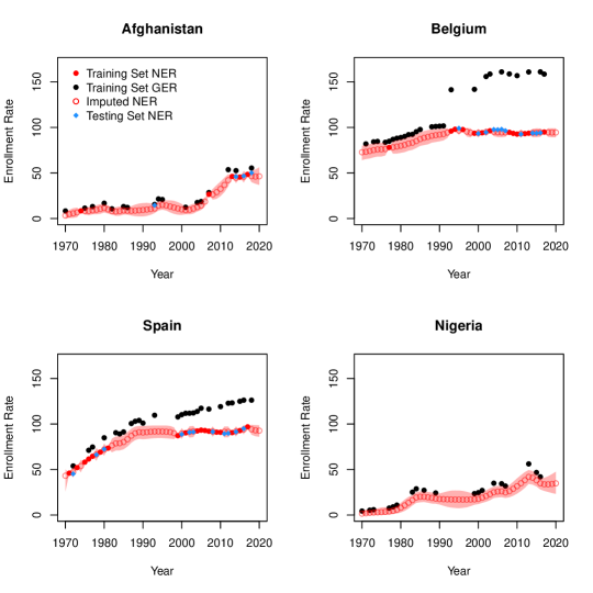
Figure 3: MCAR 40% experiment results for selected countries from the out-of-sample validation for enrollment data. Solid black and red circles indicate values in the training set for GER and NER, respectively. Solid blue diamonds indicate the true values in the testing set for NER. Open red circles indicate the median imputed values of NER and the red shaded regions indicate the 95% posterior quantiles for imputed values of NER, where values are imputed for country-years in the testing set and country-years that started as missing in the enrollment data set.

Figure 4: MAR 80% experiment results for selected countries from the out-of-sample validation for enrollment data. Solid black and red circles indicate values in the training set for GER and NER, respectively. Solid blue diamonds indicate the true values in the testing set for NER. Open red circles indicate the median imputed values of NER and the red shaded regions indicate the 95% posterior quantiles for imputed values of NER, where values are imputed for country-years in the testing set and country-years that started as missing in the enrollment data set.

5.4 Full Enrollment Data Results

We used MINTS to create 40 multiple imputations for the missing country-years in the original enrollment data set without simulating any additional country-years as missing. Figure 5 shows the multiple imputations for Afghanistan, Belgium, Spain, and Nigeria for NER as translucent red circles along with the observed values of NER and GER from the original data set in solid red and black circles, respectively. A CSV of 40 completed data sets for NER and GER created using the MINTS method and a CSV of the median imputed values for NER and GER are provided as ancillary files.

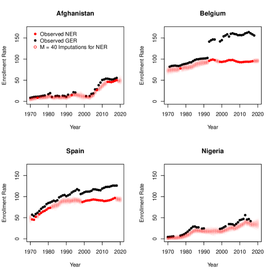
Figure 5: Results of $M=40$ imputations for NER for selected countries. Solid black and red circles indicate observed values of GER and NER, respectively, from the enrollment data set. Translucent open red circles indicate imputed values of NER, where a total of 40 imputations were created for each missing value.

6 Discussion

We developed a multiple imputation method for hierarchical time series data that can accommodate a specific type of nonlinear relationship between variables and evaluated the performance of the proposed method using a simulation study and an application to a data set on secondary school enrollment rates. Through comparisons with existing methods for multiple imputation of hierarchical time series data, we found that the proposed MINTS method can lead to substantial gains in performance when variables in the imputation model have a nonlinear relationship that can be well-approximated by a piecewise linear function.

In the simulation study, we found that MINTS performed better for estimation of parameters in uncongenial analysis models using nonlinear simulated data compared to existing models based on the MICE and Amelia methodologies. MINTS generally resulted in the smallest MAE and FMI across experiments, while retaining close to nominal coverage in all but the experiments at the highest rate of simulated missingness. The simulation study results suggest that when there is a nonlinear relationship between variables, MINTS is a preferable method over the MICE and Amelia methods. We also found MINTS still performed well when the variables in the imputation model have a linear relationship, but the difference in performance between MINTS and the existing methods was less pronounced.

For the application to the enrollment data, we evaluated how well the MINTS method performs for estimation of parameters in uncongenial analysis models and for prediction of individual missing values. Based on the analysis model validation exercises, we found that MINTS resulted in improved performance for estimation of the regression coefficient in the linear regression of TFR on NER compared to existing models based on the MICE and Amelia methodologies, with the smallest or second smallest MAE in all experiments and close to nominal coverage in all but one experiment. MINTS also had good performance for estimation of the random intercepts regression of TFR on NER at the 10% rate of simulated missingness. However at higher rates of missingness we found that the pan Random Effects method performed better for estimation of the fixed effect coefficient. At all rates of missingness, MINTS tended to have the smallest MAE for point estimation of the variance of the random intercepts. This suggests that for random intercept models, MINTS is likely to be a better choice than the existing methods if a components of variance analysis is of interest, but the pan Random Effects model could be a better choice if only the fixed effect coefficient is of interest. In the out-of-sample validation exercise for the enrollment data, we evaluated how well each imputation method predicted individual missing values for NER. We found that MINTS resulted in substantial improvements in performance compared to the existing methods, with smaller MAE, narrower intervals, and smaller interval scores across experiments. Despite the narrower intervals, MINTS still had close to nominal coverage in all experiments except MNAR 40%. Overall, our results suggest that MINTS is able to balance good predictive performance for individual missing values with good performance for multiply-imputed estimates of parameters in substantive analysis models.

To facilitate easier comparison across validation exercises, we summarize the average MAE across experiments for each multiple imputation method within each validation exercise in Table 4. A version of Table 4 that includes all validation exercises conducted is available in the Appendix. We note that Table 4 should not be interpreted as inferential and is only of interest as an exploratory comparison tool to enable a simple comparison of one metric from the full evaluation results. MINTS consistently results in the smallest average MAE across experiments in each validation exercise. Out of the previously existing imputation methods, we found the models using the pan methodology tend to have the smallest average MAE. For the validation exercises using enrollment data, the pan Random Effects method tends to perform the best out of the previously existing methods, with the second smallest average MAE for the out-of-sample validation exercise and the second or third smallest average MAE for the analysis model validation estimation of $\beta_{1}$. The pan Fixed Effects method also performs well in terms of average MAE for analysis model validation with the enrollment data, but has much larger average MAE for the out-of-sample validation exercise. For the validation exercises using the nonlinear simulated data, the pan Random Effects method has the smallest average MAE out of the existing imputation methods for estimation of $\omega_{1}$.

Table 4: Average mean absolute error (MAE) across all experiments for each multiple imputation method within each validation exercise. For the enrollment data, OOS denotes to the out-of-sample validation and $\beta_{1}$ is the parameter from the linear regression analysis model validation. For the nonlinear simulated data, $\omega_{1}$ is the parameter from the linear regression analysis model validation. MAE for the $\beta_{1}$ and $\omega_{1}$ columns are multiplied by 100 before reporting.

Method Enrollment Data Nonlinear Data OOS $\beta_{1}$ $\omega_{1}$ MICE PMM 14.68 2.97 20.16 pan Fixed 13.90 0.52 23.18 pan Random 5.36 1.48 14.30 Amelia TS 15.70 2.59 22.76 Amelia CS 9.89 2.15 37.55 Amelia TSCS 7.49 2.04 17.89 MINTS 2.77 0.18 4.15

We note that all of the imputation methods compared assume that the missing data mechanism is ignorable. We conducted sensitivity analyses to evaluate how robust each imputation model is to one type of violation of the ignorability assumption through the MNAR experiments, where the probability of a country-year being simulated as missing was dependent on the observed value. In the simulation studies, we found that all imputation methods considered were relatively robust to the violation of ignorability when the rate of simulated missingness was low. However, substantial increases in bias and undercoverage were seen at the 40% and 80% rates. MINTS tended to be the most robust to these violations for the simulated data but still suffered from bias and undercoverage, especially at the 80% rate. For the enrollment data validation exercises, no imputation method performed consistently well in the MNAR experiments. MINTS and pan Fixed Effects were the most robust to the violation of ignorability for the analysis model validation exercises, but both methods resulted in far below nominal coverage in more than one experiment. In the out-of-sample validation exercise, MINTS and pan Random Effects fared the best in the MNAR experiments. MINTS had the most robust performance in terms of point estimates, while pan Random Effects had the most robust coverage for interval estimates.

In this paper, we focused on the setting where the analysis model is uncongenial to the imputation model. This is a common occurrence for social science data, particularly when the imputation phase is conducted independently from the analysis phase. However, if the analysis of interest is known during the imputation phase, congeniality between analysis and imputation models is a worthwhile goal. Several methods have been proposed for multiple imputation of hierarchical data under congeniality where the imputation model incorporates features of the substantive analysis model, such as Goldstein et al. (2014); Enders et al. (2020); Lüdtke et al. (2020); Grund et al. (2021); among others. Of particular note, Lüdtke et al. (2020) and Grund et al. (2021) propose a method called “mdmb” that uses a sequential decomposition of the joint model. The mdmb method ensures congeniality between analysis and imputation models by incorporating a term representing the substantive analysis model into the sequential decomposition following the substantive-model-compatible philosophy of Bartlett et al. (2015).

MINTS could be extended to congeniality using the same strategy as mdmb by adding a term representing the substantive analysis model into the decomposition of the joint model as

$$p(\mathbf{Z},\mathbf{Y},\mathbf{X}|\bm{\theta}_{Z},\bm{\theta})= p(\mathbf{Z}|\mathbf{Y},\mathbf{X},\bm{\theta}_{Z})p(\mathbf{Y}|\mathbf{X},\bm{\theta}_{Y})p(\mathbf{X}|\bm{\theta}_{X}),$$

where $\mathbf{Z}$ is the outcome variable for the analysis of interest with parameters $\bm{\theta}_{Z}$. When the exact substantive analysis model of interest is included in the decomposition, MINTS could be adapted to a fully Bayesian approach and parameter estimates for the analysis model could be obtained directly from the estimation phase of the MCMC.

7 Conclusion

We have proposed the MINTS method for multiple imputation of hierarchical nonlinear time series data in the bivariate setting where one auxiliary variable is used to impute the variable of interest and the variable of interest has a larger amount of missing data than the auxiliary variable. This setting is motivated by a school enrollment rate data set from the World Bank that includes two measures of enrollment. The Net Enrollment Rate (NER) is the variable of interest for an analysis of the relationship between the Total Fertility Rate and NER, but suffers from a large amount of missing data due to the difficulty of measuring NER. A second measure of enrollment, the Gross Enrollment Ratio (GER), is easier to measure and has a smaller amount of missing data. The MINTS method leverages the strong piecewise linear relationship between NER and GER to impute missing values in both NER and GER using a combination of A-splines, country-specific intercepts, and time series methods using a sequential decomposition of the joint model.

We compared MINTS with existing methods for multiple imputation of hierarchical time series data through a simulation study and an application to the enrollment data set. We considered three models within the MICE framework of van Buuren and Groothuis-Oudshoorn (2011) and three models within the Amelia II framework of Honaker and King (2010). We found that MINTS resulted in better performance overall for estimation of parameters in uncongenial linear regression and random intercept models compared to the imputation models based on the MICE and Amelia methodologies in both a simulation study using nonlinear simulated data and the application to school enrollment data, though models based on the pan method of Schafer and Yucel (2002) were strong alternatives. We also conducted an out-of-sample validation exercise for prediction of individual missing values using the enrollment data and found that MINTS resulted in better predictive performance compared to the existing methods. Based on these validation exercises, we believe MINTS has a promising capability to improve the quality of multiply imputed data sets for hierarchical nonlinear time series data.

One limitation of the MINTS method is the use of spline estimation to model the nonlinear relationship between variables in the imputation model. The A-splines method of Goepp et al. (2018) helps to automate the estimation procedure, but as with all spline estimation methodologies there is the risk of overfitting. The MINTS algorithm uses linear splines and modifies the number of starting knots used in the A-spline algorithm when the sample size is small to reduce the risk of overfitting, but the spline estimation settings are likely to require manual tuning for applications of MINTS to other data sets. We note that other curve-fitting methods, such as LOESS, could be used instead.

MINTS also has several practical limitations compared to MICE and Amelia. Currently, MINTS is restricted to the bivariate setting with continuous variables. In principle, MINTS could be extended to the multivariate setting by adding additional univariate conditional terms to the sequential decomposition of the joint distribution, where careful consideration is needed for the ordering of the added conditional distributions. The imputation models for the added variables could be assumed to be linear or could incorporate a separate spline term for each marginal relationship in the conditional imputation model. MINTS could also be extended to accommodate categorical variables through the use of generalized regression models, for example using similar methodology as Lee and Mitra (2016). Another practical limitation of MINTS is computation time, where the estimation of the MINTS model is much more computationally intense than estimation of the MICE models and the two simpler Amelia models. Computation time could be improved by coding the MCMC algorithm in a more efficient language than R. Extending the MINTS methodology to the multivariate and mixed data type setting and improving the computational efficiency of the MINTS sampling algorithm is of interest for future work.

Appendix A Simulation of MAR and MNAR

For MAR, we assumed observations in earlier years are more likely to be missing. For each country-time pair $(c,t)$, we simulated a value $A_{c,t}$ based on $t$ with a large noise term. For the nonlinear and linear simulated data, $A_{c,t}\sim N(t,10^{2})$. For the enrollment data, $A_{c,t}\sim N(t,40^{2})$. For rate of simulated missingness $r$, we determined which values to simulate as missing based on the $r$th quantile of $\mathbf{A}$ as follows:

$$A_{boundary}= \,\text{$r$th quantile of }\bm{A}$$

$$R_{c,t}= \begin{cases}0\quad\text{if }A_{c,t}<A_{boundary}\\ 1\quad\text{otherwise}\end{cases}$$

where the response indicator $R_{c,t}$ is 0 if the observation for $(c,t)$ is missing and 1 otherwise. Missingness in $\mathbf{X}$ and $\mathbf{Y}$ was simulated independently following the method described above.

For MNAR, we simulated observations as missing depending on their observed values, where smaller values are more likely to be missing. For each $Y_{c,t}$, we first simulated a value $A_{c,t}$ based on the value of $Y_{c,t}$ with a large noise term. For the nonlinear and linear simulated data, $A_{c,t}\sim N(Y_{c,t},40^{2})$. For the enrollment data, $A_{c,t}\sim N(Y_{c,t},15^{2})$. For rate of simulated missingness $r$, we determined which values to simulate as missing based on the $r$th quantile of $\mathbf{A}$ as follows:

$$A_{boundary}= r A_{c,t}$$ th quantile of

$$R_{c,t}= \begin{cases}0\quad\text{if $A_{c,t}<A_{boundary}$}\\ 1\quad\text{otherwise}\end{cases}$$

where the response indicator $R_{c,t}$ is 0 if the observation for $(c,t)$ is missing and 1 otherwise. Missingness in $\mathbf{X}$ was simulated analogously to above, where the only difference was in the simulation of $A_{c,t}$. For the nonlinear and linear simulated data, $A_{c,t}$ for $\mathbf{X}$ was simulated as $A_{c,t}\sim N(X_{c,t},40^{2})$. For the enrollment data, $A_{c,t}$ for $\mathbf{X}$ was simulated as $A_{c,t}\sim N(X_{c,t},25^{2})$. Missingness in $\mathbf{X}$ was simulated independently of missingness in $\mathbf{Y}$.

Appendix B Data-based Control Parameters Algorithm

The control parameters for the prior distributions of the $\mathbf{X}$ model ($\delta_{X},\nu_{drift},\zeta_{drift},\text{and }\delta_{drift}$) are estimated using the observed first differences $X_{c,t}-X_{c,t-1}$ as

$$\delta_{X}= \widehat{Var}\left(X_{c,t}-X_{c,t-1}\right)$$

$$\nu_{drift}= \bar{X}_{diff}$$

$$\zeta_{drift}= SE(\bar{X}_{diff})$$

$$\delta_{drift}= \widehat{Var}(\bar{X}_{c,diff})$$

where

$$\bar{X}_{diff}= \frac{1}{n_{train}}\sum_{c,t}\left(X_{c,t}-X_{c,t-1}\right)$$

$$\bar{X}_{c,diff}= \frac{1}{n_{c}}\sum_{t}\left(X_{c,t}-X_{c,t-1}\right).$$

The control parameters for the prior distributions of the $\mathbf{Y}|\mathbf{X}$ model ($\delta_{Y},\zeta_{0},\text{and }\delta_{0}$) are estimated using the observed first differences $Y_{c,t}-Y_{c,t-1}$ as

$$\delta_{Y}= \widehat{Var}\left(Y_{c,t}-Y_{c,t-1}\right)$$

$$\zeta_{0}= SE(\bar{Y}_{diff})$$

$$\delta_{0}= \widehat{Var}(\bar{Y}_{c,diff})$$

where

$$\bar{Y}_{diff}= \frac{1}{n_{train}}\sum_{c,t}\left(Y_{c,t}-Y_{c,t-1}\right)$$

$$\bar{Y}_{c,diff}= \frac{1}{n_{c}}\sum_{t}\left(Y_{c,t}-Y_{c,t-1}\right).$$

The control parameters for the prior distributions of $(Y_{c,0},X_{c,0})$ are estimated for all $c$ as

$$\left[\begin{matrix}Y_{c,0}\\ X_{c,0}\end{matrix}\right]\sim \,TN\left(\bm{\mu}_{early},\bm{\Sigma}_{early}\right)$$

$$\bm{\mu}_{early}= \left[\begin{matrix}\bar{Y}_{early}\\ \bar{X}_{early}\end{matrix}\right]$$

$$\bm{\Sigma}_{early}= \left[\begin{matrix}\widehat{SD}(Y_{early})^{2}&\hat{r}\times\widehat{SD}(Y_{early})\times\widehat{SD}(X_{early})\\ \hat{r}\times\widehat{SD}(Y_{early})\times\widehat{SD}(X_{early})&\widehat{SD}(X_{early})^{2}\end{matrix}\right]$$

The prior mean and covariance matrix are calculated using the sample means $\bar{Y}_{early}$ and $\bar{X}_{early}$, sample standard deviations $\widehat{SD}(Y_{early})$ and $\widehat{SD}(X_{early})$, and the sample Pearson correlation coefficient $\hat{r}$ for a subset of the data $(\mathbf{Y}_{early},\mathbf{X}_{early})$ that consists of all complete cases $(Y_{c,t},X_{c,t})$ in “early” times. The time range determined to be “early” is based on availability of the observed complete cases. For the enrollment data, $(\mathbf{Y}_{early},\mathbf{X}_{early})$ consists of all country-time pairs in years 1970-1980 (corresponding to $t=1,...,11$) where both $Y_{c,t}$ and $X_{c,t}$ were observed. The truncation was specified as $X_{c,0}\in[0,min(X_{c,obs})]$ and $Y_{c,0}\in[0,min(Y_{c,obs})]$, where $min(X_{c,obs})$ is the minimum observed value of $X$ for country $c$ and $min(Y_{c,obs})$ is the minimum observed value of $Y$ for country $c$.

Appendix C MCMC Algorithm

The MCMC algorithm for the MINTS method uses univariate Gibbs sampling steps for most imputation model parameters combined with a Metropolis-within-Gibbs step for the parameter block $(\beta,\rho)$. Let $\bm{\theta}=(\bm{\theta}_{X},\bm{\theta}_{Y})$ denote the vector of all parameters in the imputation model, where $\bm{\theta}_{X}=(\bm{\gamma},\sigma_{X}^{2},\mathbf{X}_{0},\mu_{drift},\sigma^{2}_{drift})$ and $\bm{\theta}_{Y}=(\bm{\alpha},\beta,\rho,\sigma_{Y}^{2},\mathbf{Y}_{0},\mu_{0},\sigma^{2}_{0})$. Let $n=C\times T$ denote the total number of country-years. Let the hyperparameters for the joint distribution of $\mathbf{X}_{0}$ and $\mathbf{Y}_{0}$ be written as

$$\bm{\mu}_{early}= \left[\begin{matrix}\mu_{Y,early}\\ \mu_{X,early}\end{matrix}\right],\quad\bm{\Sigma}_{early}=\left[\begin{matrix}\sigma_{Y,early}^{2}&r\times\sigma_{Y,early}\sigma_{X,early}\\ r\times\sigma_{Y,early}\sigma_{X,early}&\sigma_{X,early}^{2}\end{matrix}\right].$$

To simplify notation, let $\mathbf{X}^{(i)}=(\mathbf{X}_{obs},\mathbf{X}_{mis}^{(i)})$ represent the vector of the observed portion of $\mathbf{X}$ and the imputed values for $\mathbf{X}_{mis}$ from the $i$th iteration. Similarly, let $\mathbf{Y}^{(i)}=(\mathbf{Y}_{obs},\mathbf{Y}_{mis}^{(i)})$.

Each chain of the MCMC is initialized with starting values $\bm{\theta}_{X}^{(0)}$ and $\bm{\theta}_{Y}^{(0)}$ randomly drawn from diffuse distributions modeled after the prior distributions. Initial values for the missing observations are constructed using a combination of linear interpolation of the observed values, predicted values from the spline $f$, and constant extrapolation. In each chain, starting values $\mathbf{X}_{mis}^{(0)}$ and $\mathbf{Y}_{mis}^{(0)}$ are randomly drawn from normal distributions centered at the previously constructed initial values.

For each chain, the MCMC sampling algorithm then proceeds as follows for iterations $i=1,...,.n_{iter}$:

1. $\sigma_{Y}^{2,(i)}$ is sampled from

   $$\begin{split}\sigma_{Y}^{2}|&\beta^{(i-1)},\rho^{(i-1)},\bm{\alpha}^{(i-1)},\mathbf{X}_{0}^{(i-1)},\mathbf{Y}_{0}^{(i-1)},\mathbf{X}^{(i-1)},\mathbf{Y}^{(i-1)}\\ \sim&InvGamma\Bigg{(}2+\frac{n}{2},\Bigg{.}\\ &\qquad\Bigg{.}\delta_{Y}+\frac{1}{2}\sum_{t=1}^{T}\left(\frac{1}{h(\mathbf{X}_{t}^{(i-1)})}\left(\mathbf{Y}_{t}^{(i-1)}-\rho^{(i-1)}\mathbf{Y}_{t-1}^{(i-1)}-\bm{\alpha}^{(i-1)}-\beta^{(i-1)}f(\mathbf{X}_{t}^{(i-1)}\right)^{2}\right)\Bigg{)}.\end{split}$$

2. The parameters $(\beta^{(i)},\rho^{(i)})$ are sampled as a block using a Metropolis-Hastings step. Values $\beta_{new}$ and $\rho_{new}$ are drawn from the proposal function given by the truncated bivariate normal distribution

   $$TN\left(\left[\begin{matrix}\beta^{(i-1)}\\ \rho^{(i-1)}\end{matrix}\right],\phi\left[\begin{matrix}0.001475944&-0.001511349\\ -0.001511349&0.001577437\end{matrix}\right]\right),$$

   where the tuning parameter $\phi$ for the covariance matrix is determined following a pilot run of the MCMC to ensure the acceptance rate is around 40% and the truncation is such that $\beta\in(-\infty,\infty)$ and $\rho\in[0,1]$.

   The acceptance ratio is calculated as

   $$\frac{p(\mathbf{Y}^{(i-1)}|\mathbf{X}^{(i-1)},\mathbf{Y}_{0}^{(i-1)},\bm{\alpha}^{(i-1)},\sigma_{Y}^{2,(i)},\beta_{new},\rho_{new})}{p(\mathbf{Y}^{(i-1)}|\mathbf{X}^{(i-1)},\mathbf{Y}_{0}^{(i-1)},\bm{\alpha}^{(i-1)},\sigma_{Y}^{2,(i)},\beta^{(i-1)},\rho^{(i-1)})}$$

   $$\,=\exp\left[\sum_{t=1}^{T}\frac{-\left(\mathbf{Y}_{t}^{(i-1)}-\bm{\alpha}^{(i-1)}-\beta^{new}f(\mathbf{X}_{t}^{(i-1)})-\rho^{new}\mathbf{Y}_{t-1}^{(i-1)}\right)^{2}}{2\sigma_{Y}^{2,(i)}h(\mathbf{X}_{t}^{(i-1)})}\right.$$

   $$\qquad\qquad\left.-\sum_{t=1}^{T}\frac{-\left(\mathbf{Y}_{t}^{(i-1)}-\bm{\alpha}^{(i-1)}-\beta^{(i-1)}f(\mathbf{X}_{t}^{(i-1)})-\rho^{(i-1)}\mathbf{Y}_{t-1}^{(i-1)}\right)^{2}}{2\sigma_{Y}^{2,(i)}h(\mathbf{X}_{t}^{(i-1)})}\right].$$

3. $\sigma_{X}^{2,(i)}$ is sampled from

   $$\sigma_{X}^{2}| \bm{\gamma}^{(i-1)},\mathbf{X}_{0}^{(i-1)},\mathbf{X}^{(i-1)}$$

   $$\sim InvGamma\Bigg{(}2+\frac{n}{2},\delta_{X}+\frac{1}{2}\sum_{t=1}^{T}\left(\mathbf{X}_{t}^{(i-1)}-\mathbf{X}_{t-1}^{(i-1)}-\bm{\gamma}^{(i-1)}\right)^{2}\Bigg{)}.$$

4. To sample the country-specific drift terms $\gamma_{c}^{(i)}$, the hyperparameters $\mu_{drift}^{(i)}$ and $\sigma^{2,(i)}_{drift}$ are first sampled from

   $$\mu_{drift}^{(i)}|\sigma_{drift}^{2,(i-1)},\bm{\gamma}^{(i-1)}\sim N\left(\left(\frac{1}{\zeta_{drift}^{2}}+\frac{C}{\sigma_{drift}^{2,(i-1)}}\right)^{-1}\left(\frac{\nu_{drift}}{\zeta_{drift}^{2}}+\sum_{c=1}^{C}\frac{\gamma_{c}^{(i-1)}}{\sigma_{drift}^{2,(i-1)}}\right),\left(\frac{1}{\zeta_{drift}^{2}}+\frac{C}{\sigma_{drift}^{2,(i-1)}}\right)^{-1}\right)$$

   $$\sigma_{drift}^{2,(i)}|\mu_{drift}^{(i)},\bm{\gamma}^{(i-1)}\sim InvGamma\left(2+\frac{C}{2},\delta_{drift}+\frac{1}{2}\sum_{c=1}^{C}\left(\gamma_{c}^{(i-1)}-\mu_{drift}^{(i)}\right)^{2}\right).$$

   For each $c$, $\gamma_{c}^{(i)}$ is sampled from

   $$\gamma_{c}^{(i)}| \mu_{drift}^{(i)},\sigma^{2,(i)}_{drift},\sigma_{X}^{2,(i)},\mathbf{X}_{0}^{(i-1)},\mathbf{X}^{(i-1)}$$

   $$\sim N\left(\left(\frac{1}{\sigma^{2,(i)}_{drift}}+\frac{T}{\sigma_{X}^{2,(i)}}\right)^{-1}\left(\frac{\mu_{drift}^{(i)}}{\sigma^{2,(i)}_{drift}}+\sum_{t=1}^{T}\frac{X_{c,t}^{(i-1)}-X_{c,t-1}^{(i-1)}}{\sigma_{X}^{2,(i)}}\right),\left(\frac{1}{\sigma^{2,(i)}_{drift}}+\frac{T}{\sigma_{X}^{2,(i)}}\right)^{-1}\right).$$

5. To sample the country-specific random intercept terms $\alpha_{c}^{(i)}$, the hyperparameters $\mu_{0}^{(i)}$ and $\sigma_{0}^{2,(i)}$ are first sampled from

   $$\mu_{0}^{(i)}|\sigma_{0}^{2,(i-1)},\bm{\alpha}^{(i-1)}\sim N\left(\left(\frac{1}{\zeta_{0}^{2}}+\frac{C}{\sigma_{0}^{2,(i-1)}}\right)^{-1}\left(\frac{\nu_{0}}{\zeta_{0}^{2}}+\sum_{c=1}^{C}\frac{\alpha_{c}^{(i-1)}}{\sigma_{0}^{2,(i-1)}}\right),\left(\frac{1}{\zeta_{0}^{2}}+\frac{C}{\sigma_{0}^{2,(i-1)}}\right)^{-1}\right)$$

   $$\sigma_{0}^{2,(i)}|\mu_{0}^{(i)},\bm{\alpha}^{(i-1)}\sim InvGamma\left(2+\frac{C}{2},\delta_{0}+\frac{1}{2}\sum_{c=1}^{C}\left(\alpha_{c}^{(i-1)}-\mu_{0}^{(i)}\right)^{2}\right).$$

   For each $c$, $\alpha_{c}^{(i)}$ is sampled from

   $$\alpha_{c}^{(i)}| \mu_{0}^{(i)},\sigma^{2,(i)}_{0},\sigma_{Y}^{2,(i)},\mathbf{Y}_{0}^{(i-1)},\mathbf{Y}^{(i-1)},\mathbf{X}^{(i-1)}$$

   $$\sim N\left(\left(\frac{1}{\sigma^{2,(i)}_{0}}+\sum_{t=1}^{T}\frac{1}{\sigma_{Y}^{2,(i)}h(X_{c,t}^{(i-1)})}\right)^{-1}\left(\frac{\mu_{0}^{(i)}}{\sigma^{2,(i)}_{0}}+\sum_{t=1}^{T}\frac{Y_{c,t}^{(i-1)}-\rho^{(i)}Y_{c,t-1}^{(i-1)}-\beta^{(i)}f(X_{c,t}^{(i-1)})}{\sigma_{Y}^{2,(i)}h(X_{c,t}^{(i-1)})}\right),\right.$$

   $$\qquad\left.\left(\frac{1}{\sigma^{2,(i)}_{0}}+\sum_{t=1}^{T}\frac{1}{\sigma_{Y}^{2,(i)}h(X_{c,t}^{(i-1)})}\right)^{-1}\right).$$

6. Imputed values for each missing value in $\mathbf{X}_{mis}^{(i)}$ are drawn for each country in descending order by year. For all $X_{c,t}$ that are observed, we set $X_{c,t}^{(i)}=X_{c,t}$ for all iterations $i$. For $t=T$, the imputed value for $X_{c,t}^{(i)}$ is drawn from

   $$X_{c,T}^{(i)}|\gamma_{c}^{(i)},\sigma_{X}^{2,(i)},X_{c,T-1}^{(i-1)}\sim TN_{[X_{low},X_{up}]}\left(X_{c,T-1}^{(i-1)}+\gamma_{c}^{(i)},\sigma_{X}^{2,(i)}\right).$$

   For $t<T$, the imputed value for $X_{c,t}^{(i)}$ is drawn in descending order from largest $t$ to smallest $t$ from

   $$X_{c,t}^{(i)}|\gamma_{c}^{(i)},\sigma_{X}^{2,(i)},X_{c,t+1}^{(i)},X_{c,t-1}^{(i-1)}\sim TN_{[X_{low},X_{up}]}\left(\frac{X_{c,t+1}^{(i)}+X_{c,t-1}^{(i-1)}}{2},\frac{\sigma_{X}^{2,(i)}}{2}\right).$$

7. $X_{c,0}^{(i)}$ is sampled from

   $$X_{c,0}^{(i)}| \gamma_{c}^{(i)},\sigma_{X}^{2,(i)},\bm{\mu}_{early},\bm{\Sigma}_{early},X_{c,1}^{(i)}$$

   $$\sim TN_{[X_{0,low},X_{0,up}]}\left(\left(\frac{1}{\sigma_{X}^{2,(i)}}+\frac{1}{\sigma_{X,early}^{2}}\right)^{-1}\left(\frac{X_{c,1}^{(i)}-\gamma_{c}^{(i)}}{\sigma_{X}^{2,(i)}}+\frac{\mu_{X,early}}{\sigma_{X,early}^{2}}\right),\right.$$

   $$\qquad\qquad\qquad\qquad\left.\left(\frac{1}{\sigma_{X}^{2,(i)}}+\frac{1}{\sigma_{X,early}^{2}}\right)^{-1}\right).$$

8. Imputed values for each missing value in $\mathbf{Y}_{mis}^{(i)}$ are drawn for each country in descending order by year. For all $Y_{c,t}$ that are observed, we set $Y_{c,t}^{(i)}=Y_{c,t}$ for all iterations $i$. For $t=T$, the imputed value for $Y_{c,t}^{(i)}$ is drawn from

   $$Y_{c,T}^{(i)}|\alpha_{c}^{(i)},\rho^{(i)},\beta^{(i)},\sigma_{Y}^{2,(i)},Y_{c,T-1}^{(i-1)},X_{c,T}^{(i)}\sim TN_{[Y_{low},Y_{up}]}\left(\alpha_{c}^{(i)}+\rho^{(i)}Y_{c,T-1}^{(i-1)}+\beta^{(i)}f(X_{c,T}^{(i)}),\sigma_{Y}^{2,(i)}h(X_{c,T}^{(i)})\right).$$

   For $t<T$, the imputed value for $Y_{c,t}^{(i)}$ is drawn in descending order from largest $t$ to smallest $t$ from

   $$Y_{c,t}^{(i)}| \alpha_{c}^{(i)},\rho^{(i)},\beta^{(i)},\sigma_{Y}^{2,(i)},Y_{c,t+1}^{(i)},Y_{c,t-1}^{(i-1)},X_{c,t}^{(i)},X_{c,t+1}^{(i)}$$

   $$\sim TN_{[Y_{low},Y_{up}]}\left(\left(\frac{(\rho^{(i)})^{2}}{\sigma_{Y}^{2,(i)}h(X_{c,t+1}^{(i)})}+\frac{1}{\sigma_{Y}^{2,(i)}h(X_{c,t}^{(i)})}\right)^{-1}\left(\frac{\rho^{(i)}(Y_{c,t+1}^{(i)}-\alpha_{c}^{(i)}-\beta^{(i)}f(X_{c,t+1}^{(i)}))}{\sigma_{Y}^{2,(i)}h(X_{c,t+1}^{(i)})}\right.\right.$$

   $$\qquad\qquad\qquad\left.\left.+\frac{\rho^{(i)}Y_{c,t-1}^{(i-1)}+\alpha_{c}^{(i)}+\beta^{(i)}f(X_{c,t}^{(i)})}{\sigma_{Y}^{2,(i)}h(X_{c,t}^{(i)})}\right),\left(\frac{(\rho^{(i)})^{2}}{\sigma_{Y}^{2,(i)}h(X_{c,t+1}^{(i)})}+\frac{1}{\sigma_{Y}^{2,(i)}h(X_{c,t}^{(i)})}\right)^{-1}\right).$$

9. $Y_{c,0}^{(i)}$ is sampled from

   $$Y_{c,0}^{(i)}| \alpha_{c}^{(i)},\rho^{(i)},\beta^{(i)},\sigma_{Y}^{2,(i)},X_{c,0}^{(i)},\bm{\mu}_{early},\bm{\Sigma}_{early},Y_{c,1}^{(i)},X_{c,1}^{(i)}$$

   $$\sim TN_{[Y_{0,low},Y_{0,up}]}\left(\left(\frac{(\rho^{(i)})^{2}}{\sigma_{Y}^{2,(i)}h(X_{c,1}^{(i)})}+\frac{1}{(1-r^{2})\sigma_{Y,early}^{2}}\right)^{-1}\left(\frac{\rho^{(i)}(Y_{c,1}^{(i)}-\alpha_{c}^{(i)}-\beta^{(i)}f(X_{c,1}^{(i)}))}{\sigma_{Y}^{2,(i)}h(X_{c,1}^{(i)})}\right.\right.$$

   $$\qquad\qquad\qquad\left.\left.+\frac{\mu_{Y,early}+\frac{r\sigma_{Y,early}}{\sigma_{X,early}}(X_{c,0}^{(i)}-\mu_{X,early})}{(1-r^{2})\sigma_{Y,early}^{2})}\right),\left(\frac{(\rho^{(i)})^{2}}{\sigma_{Y}^{2,(i)}h(X_{c,1}^{(i)})}+\frac{1}{(1-r^{2})\sigma_{Y,early}^{2}}\right)^{-1}\right).$$

Appendix D Analysis Model Validation for Random Intercept Analysis Models

For both the simulated data and the school enrollment data, we considered a second analysis model validation exercise using random intercept models as the analysis models.

D.1 Nonlinear Data

For the nonlinear simulated data, the second model used for analysis model validation is the random intercept model given by

$$Z_{c,t}= \,\lambda_{0}+\lambda_{c}+\lambda_{1}Y_{c,t}+\varepsilon_{c,t}^{\lambda},$$

$$\lambda_{c}\sim N(0,\sigma_{\lambda}^{2}),$$

$$\varepsilon_{c,t}^{\lambda}\sim N(0,\sigma_{\varepsilon_{\lambda}}^{2}).$$

The parameter of interest in the fixed component of the model is the coefficient $\lambda_{1}$, while the parameter of interest in the random component of the model is the variance of the random intercepts $\sigma_{\lambda}^{2}$.

Table 5: Summary of analysis model validation for nonlinear simulated data for $Q=\lambda_{1}$, the fixed effect coefficient coefficient on $Y$ in the random intercept model of $Z$ on $Y$. MAE denotes mean absolute error, Cvg denotes the average coverage of 95% intervals as a percentage, and FMI denotes the fraction of missing information as a percentage. MAE is multiplied by 100 before reporting. Results are averaged over the 1000 replications of each experiment. The true value of $Q$ is 2.028.

Simulated Method MCAR MAR MNAR Missingness Rate MAE Cvg FMI MAE Cvg FMI MAE Cvg FMI 10% MICE PMM 1.23 100.0 8.2 0.51 100.0 4.3 0.78 100.0 5.8 pan Fixed 1.94 100.0 6.4 6.23 92.6 7.6 3.49 100.0 5.9 pan Random 1.27 100.0 4.2 5.71 97.3 5.9 2.58 100.0 4.0 Amelia TS 2.46 100.0 8.2 6.00 99.3 9.5 3.86 100.0 7.4 Amelia CS 2.59 100.0 9.0 6.49 98.4 10.2 3.93 100.0 7.6 Amelia TSCS 1.34 100.0 4.9 5.96 95.2 6.6 2.65 100.0 4.3 MINTS 0.30 100.0 0.6 0.59 100.0 0.7 0.31 100.0 0.5 40% MICE PMM 18.44 2.9 43.4 5.34 99.8 27.0 12.53 28.6 38.9 pan Fixed 11.33 44.5 26.2 24.39 0.0 23.6 17.12 0.1 23.6 pan Random 5.18 96.4 18.1 22.16 0.0 18.5 10.51 19.7 17.4 Amelia TS 17.37 1.7 26.8 26.20 0.0 25.4 20.60 0.0 25.7 Amelia CS 22.81 0.0 32.2 25.50 0.0 24.4 22.48 0.0 26.4 Amelia TSCS 5.35 95.9 23.1 23.04 0.0 26.5 10.48 22.4 19.9 MINTS 1.22 100.0 4.2 3.08 99.8 5.9 1.48 100.0 3.4 80% MICE PMM 65.74 0.0 59.5 38.43 0.0 58.5 66.21 0.0 55.2 pan Fixed 39.27 1.7 50.1 46.31 0.0 38.8 48.62 0.0 45.2 pan Random 12.16 64.8 53.0 38.72 0.0 44.8 24.48 2.8 53.0 Amelia TS 50.51 1.2 51.5 62.36 0.0 34.9 54.86 0.0 34.4 Amelia CS 99.78 0.0 56.5 76.22 0.0 66.9 75.86 0.0 48.9 Amelia TSCS 19.10 71.4 77.9 41.71 0.0 64.5 29.87 10.7 74.6 MINTS 7.53 82.0 39.9 10.74 59.8 45.7 9.54 66.4 37.5

We first evaluated how well each method performs for estimation of $Q=\lambda_{1}$, the fixed effect coefficient on $\mathbf{Y}$. Table 5 summarizes the results of this validation for the nonlinear simulated data. Overall, the validation results for estimation of the fixed effect coefficient are similar to the results for the linear regression analysis model. MINTS has the smallest MAE in all experiments except MAR 10%, where MICE PMM has slightly smaller MAE. MINTS also has generally good coverage and small FMI across experiments. While coverage is poor for all methods at the 80% rate, MINTS has the closest to nominal coverage. Out of the existing methods, MICE PMM has good performance for the experiments at the lower rates of missingness but performs poorly at the 80% rate. Pan Random Effects and Amelia TSCS have the best overall performance out of the existing methods that are specifically designed for hierarchical time series data, particularly in the experiments where the missing data mechanism is MCAR. However, both pan Random Effects and Amelia TSCS have worse performance than MINTS.

Next, we evaluated the MAE for estimation of $Q=\sigma_{\lambda}^{2}$, the variance of the random intercepts. Table 6 summarizes the results of this validation exercise for the nonlinear simulated data. We find MINTS has the smallest MAE in all experiments except one. In the MAR 80% experiment, pan Fixed Effects has the smallest MAE and MINTS has the second smallest MAE.

Table 6: Mean absolute error for the analysis model validation for nonlinear simulated data for $Q=\sigma_{\lambda}^{2}$, the variance of the random intercepts in the random intercept model of $Z$ on $Y$. Results are averaged over the 1000 replications of each experiment. The true value of $Q$ is 13.615.

Simulated Method MCAR MAR MNAR Missingness Rate 10% MICE PMM 0.74 0.66 0.70 pan Fixed 0.74 0.78 0.72 pan Random 0.62 0.97 0.62 Amelia TS 0.79 0.62 0.67 Amelia CS 1.08 1.09 0.86 Amelia TSCS 0.68 1.13 0.67 MINTS 0.20 0.23 0.21 40% MICE PMM 9.09 1.43 3.65 pan Fixed 2.87 1.83 1.71 pan Random 2.10 5.64 2.08 Amelia TS 10.62 4.71 6.06 Amelia CS 8.73 2.54 3.06 Amelia TSCS 2.24 6.76 2.22 MINTS 0.55 0.57 0.56 80% MICE PMM 87.57 46.12 66.55 pan Fixed 21.94 7.44 8.83 pan Random 15.00 19.42 12.00 Amelia TS 74.74 54.60 52.99 Amelia CS 73.50 24.74 36.57 Amelia TSCS 30.03 52.60 36.35 MINTS 5.44 7.91 4.24

D.2 Enrollment Data

Table 7: Summary of analysis model validation for enrollment data for $Q=\psi_{1}$, the fixed effect coefficient on NER in the random intercept model of TFR on NER. MAE denotes mean absolute error, Cvg denotes the average coverage of 95% intervals as a percentage, and FMI denotes the fraction of missing information as a percentage. MAE is multiplied by 100 before reporting. Results are averaged over the 100 replications of each experiment. The value of $Q$ estimated using the observed country-years from the full enrollment data set is -0.058.

Simulated Method MCAR MAR MNAR Missingness Rate MAE Cvg FMI MAE Cvg FMI MAE Cvg FMI 10% MICE PMM 1.66 5 36.2 1.98 0 42.6 7.01 0 26.4 pan Fixed 0.23 100 17.4 0.18 100 17.7 2.63 0 34.8 pan Random 0.18 100 14.8 0.20 100 16.6 1.96 0 48.5 Amelia TS 1.42 19 34.9 1.74 3 38.5 6.96 0 27.6 Amelia CS 0.66 87 20.5 0.89 70 23.0 5.07 0 42.3 Amelia TSCS 0.20 99 22.6 0.23 100 23.8 4.23 0 86.0 MINTS 0.13 100 8.2 0.14 100 7.1 0.66 67 18.6 40% MICE PMM 4.09 0 40.0 4.23 0 45.0 5.32 0 44.9 pan Fixed 0.56 50 28.6 0.28 93 29.1 0.13 100 38.6 pan Random 0.17 98 36.2 0.17 100 41.1 1.20 43 72.1 Amelia TS 3.83 0 38.0 4.00 0 41.2 5.19 0 44.3 Amelia CS 2.27 0 35.9 2.44 0 34.2 5.19 0 44.3 Amelia TSCS 0.22 100 59.6 0.25 100 66.5 3.31 10 91.8 MINTS 0.30 83 17.2 0.27 90 18.6 0.74 2 49.8 80% MICE PMM 4.87 0 61.4 5.03 0 63.1 pan Fixed 1.36 0 51.3 0.82 15 54.4 pan Random 0.36 93 69.6 0.23 100 72.8 Amelia TS 4.70 0 50.8 4.85 0 56.4 Amelia CS 4.09 0 47.2 3.91 0 44.7 Amelia TSCS 1.48 30 86.9 2.34 8 88.3 MINTS 0.55 17 44.5 0.50 22 45.0

For the secondary school enrollment data, the second model used for analysis model validation is the random intercept model of TFR on NER given by

$$\text{TFR}_{c,t}= \psi_{0}+\psi_{c}+\psi_{1}\text{NER}_{c,t}+\varepsilon_{c,t}^{\psi},$$

$$\psi_{c}\sim N(0,\sigma_{\psi}^{2}),$$

$$\varepsilon_{c,t}^{\psi}\sim N(0,\sigma_{\varepsilon_{\psi}}^{2}).$$

The parameter of interest in the fixed component of the model is the coefficient $\psi_{1}$, while the parameter of interest in the random component of the model is the variance of the random intercepts $\sigma_{\psi}^{2}$. For each replication of each experiment, the analysis model is estimated using only the country-years that were simulated as missing and where TFR $>2.5$.

Table 7 summarizes the results of the analysis model validation for estimation of $Q=\psi_{1}$, the fixed effect coefficient on NER in the random intercept model. MINTS has the best performance for estimation of $\psi_{1}$ at the 10% rate, with the smallest MAE, smallest FMI, and closest to nominal coverage. For most of the experiments at the 40% and 80% rates, pan Random Effects has the best performance for estimation of $\psi_{1}$ with the smallest MAE and closest to nominal coverage. The one exception is MNAR 40%, where the pan Fixed Effects method outperforms pan Random Effects. MINTS has the second or third smallest MAE in the 40% and 80% experiments for estimation of $\psi_{1}$, but suffers from undercoverage.

Table 8 summarizes the results of the analysis model validation for point estimation of $Q=\sigma_{\psi}^{2}$, the variance of the random intercepts. We find MINTS results in the smallest MAE across all experiments.

Table 8: Mean absolute error for the analysis model validation for enrollment data for $Q=\sigma_{\psi}^{2}$, the variance of the random intercepts in the random intercept model of TFR on NER. Results are averaged over the 100 replications of each experiment. The value of $Q$ estimated using the observed country-years from the full enrollment data set is 1.004.

Simulated Method MCAR MAR MNAR Missingness Rate 10% MICE PMM 0.12 0.12 0.51 pan Fixed 0.09 0.09 0.20 pan Random 0.05 0.06 0.60 Amelia TS 0.13 0.12 0.50 Amelia CS 0.11 0.13 0.50 Amelia TSCS 0.08 0.13 0.67 MINTS 0.03 0.03 0.04 40% MICE PMM 0.20 0.20 0.52 pan Fixed 0.18 0.15 0.37 pan Random 0.07 0.11 2.23 Amelia TS 0.17 0.19 0.49 Amelia CS 0.15 0.15 0.53 Amelia TSCS 0.17 0.32 0.99 MINTS 0.06 0.04 0.12 80% MICE PMM 0.41 0.41 pan Fixed 0.21 0.21 pan Random 1.05 1.36 Amelia TS 0.38 0.39 Amelia CS 0.12 0.12 Amelia TSCS 0.28 0.32 MINTS 0.11 0.09

Appendix E Simulation Study for Linear Data

We conducted a simulation study to evaluate how well the multiply imputed data sets from the proposed imputation method perform for estimation of quantities of interest $Q$, where the quantities considered are parameters from analysis models that are uncongenial to the imputation model. We refer to this validation exercise as “analysis model validation.”

Analysis model validation was conducted for two simulated data sets: one with a nonlinear relationship between $\mathbf{X}$ and $\mathbf{Y}$ and one with a linear relationship. For each simulated data set, we simulated missingness following three rates of simulated missingness (10%, 40%, 80%) and three missing data mechanisms for a total of nine experiments. Each experiment was replicated $N_{rep}=1000$ times and the average performance of the proposed imputation method was compared with the performance of existing multiple imputation methods for hierarchical time series data. This section describes the simulation study using linear simulated data.

E.1 Data Generation

Variables $\mathbf{X}$ and $\mathbf{Y}$ are simulated following a hierarchical time series structure where the grouping variable is country and the time variable is year. We simulated data for 20 countries and 30 years for a total sample size of 600 country-year pairs. We assume $\mathbf{Y}$ is the variable of interest for substantive analyses, while $\mathbf{X}$ is an auxiliary variable that is only of interest for imputation of $\mathbf{Y}$.

Values of $\mathbf{X}$ were simulated independently for each country as follows. $\mathbf{X}$ is assumed to be generally increasing over time and is truncated to be bounded in $[0,100]$. For country $c$,

$$X_{c,1}\sim \,U(X_{1,low},X_{1,up})$$

$$X_{c,t+1}\sim \,TN_{[0,100]}(X_{c,t}+\gamma_{c},\sigma^{2})\text{ for $t=1,...,29$}$$

where $TN_{[0,100]}$ refers to the truncated normal distribution with support $[0,100]$ and $\gamma_{c}$ is a country-specific drift term. For the linear simulated data, $\mathbf{X}$ is simulated using $X_{1,low}=2$, $X_{1,up}=20$, $\sigma^{2}=2$, and $\gamma_{c}\sim N(2,0.5^{2})$.

$\mathbf{Y}$ was simulated to have a linear relationship with $\mathbf{X}$ and to be bounded as $Y_{c,t}\in[0,\text{min}(X_{c,t},100)]$. For country $c$,

$$Y_{c,t}\sim \,TN_{[0,\text{min}(X_{c,t},100)]}\left(\alpha_{c}+0.75X_{c,t},1^{2}\right)$$

$$\alpha_{c}\sim \,U(0,5)$$

where $TN_{[0,\text{min}(X_{c,t},100)]}$ refers to the truncated normal distribution with support $[0,\text{min}(X_{c,t},100)]$.

E.2 Analysis Models

For the analysis model validation exercises, we focus on the setting where the analysis model is uncongenial to the imputation model. The same methodology is used to construct the outcome variable and the analysis models for the nonlinear and linear simulated data experiments. We simulated a variable $\mathbf{Z}$ that acts as the outcome variable for the analysis models. $\mathbf{Z}$ is simulated to have a linear relationship with $\mathbf{Y}$ as follows:

$$Z_{c,t}\sim \,N(\eta_{c}+2Y_{c,t},10^{2})$$

$$\eta_{c}\sim \,U(0,15).$$

We considered two analysis models to model the relationship between $\mathbf{Z}$ and $\mathbf{Y}$. The first analysis model is the linear regression of $\mathbf{Z}$ on $\mathbf{Y}$, where the parameter of interest for estimation is $\omega_{1}$, the coefficient on $\mathbf{Y}$ in the regression

$$Z_{c,t}= \,\omega_{0}+\omega_{1}Y_{c,t}+\varepsilon_{c,t}$$

$$\varepsilon_{c,t}\sim N(0,\sigma_{\varepsilon}^{2}).$$

The second analysis model is the random intercept model given by

$$Z_{c,t}= \,\lambda_{0}+\lambda_{c}+\lambda_{1}Y_{c,t}+\varepsilon_{c,t}$$

$$\lambda_{c}\sim N(0,\sigma_{\lambda}^{2})$$

$$\varepsilon_{c,t}\sim N(0,\sigma_{\varepsilon}^{2}),$$

where we have two parameters of interest. The parameter of interest in the fixed component of the model is the coefficient $\lambda_{1}$. The parameter of interest in the random component of the model is the variance of the random intercepts $\sigma_{\lambda}^{2}$.

E.3 Analysis Model Validation Procedure and Model Implementation

The same analysis model validation procedure and model implementations were used for the linear simulated data as were used for the nonlinear simulated data. The only differences occur with the bounds of the different imputation models. For the MINTS model, the bounds for the $\mathbf{Y}|\mathbf{X}$ model were set as $Y_{low}=0$ and $Y_{up}=\text{min}(X_{c,t},100)$ for the linear simulated data. For the models using the “mice” and “Amelia” R packages, the bounds were set as $\mathbf{X}\in[0,100]$ and $\mathbf{Y}\in[0,100]$.

E.4 Analysis Model Validation Results

For the linear regression analysis model validation, we evaluate how well each multiple imputation method performs for estimation of $Q=\omega_{1}$, the regression coefficient on $\mathbf{Y}$ in the linear regression of $\mathbf{Z}$ on $\mathbf{Y}$.

Table 9: Summary of uncongenial analysis model validation for linear simulated data for $Q=\omega_{1}$, the regression coefficient on $Y$ in the linear regression of $Z$ on $Y$. MAE denotes mean absolute error, Cvg denotes the average coverage of 95% intervals as a percentage, and FMI denotes the fraction of missing information as a percentage. MAE is multiplied by 100 before reporting. Results are averaged over the 1000 replications of each experiment. The true value of $Q$ is 2.019.

Simulated Method MCAR MAR MNAR Missingness Rate MAE Cvg FMI MAE Cvg FMI MAE Cvg FMI 10% MICE PMM 3.32 100.0 48.8 1.68 100.0 14.1 2.95 100.0 41.9 pan Fixed 0.67 100.0 6.6 2.32 100.0 22.0 1.46 100.0 16.1 pan Random 0.61 100.0 2.9 1.87 100.0 3.9 0.88 100.0 2.8 Amelia TS 0.74 100.0 4.7 1.06 100.0 5.8 0.74 100.0 4.6 Amelia CS 1.44 100.0 11.4 4.34 99.9 26.3 2.16 100.0 16.5 Amelia TSCS 0.19 100.0 0.7 0.58 100.0 1.3 0.23 100.0 0.7 MINTS 0.16 100.0 0.6 0.22 100.0 0.8 0.16 100.0 0.6 40% MICE PMM 13.18 55.9 64.6 7.28 93.7 51.3 14.32 63.9 73.7 pan Fixed 5.18 95.9 33.5 16.68 0.0 54.8 9.94 23.9 48.7 pan Random 1.80 100.0 16.2 5.95 58.9 20.8 2.74 100.0 14.3 Amelia TS 8.74 45.1 27.2 11.22 0.7 27.5 10.88 3.9 27.3 Amelia CS 22.35 0.0 40.7 39.73 0.0 43.3 28.50 0.0 43.0 Amelia TSCS 1.02 100.0 7.6 5.05 78.8 15.0 1.86 100.0 8.7 MINTS 0.68 100.0 6.4 1.11 99.7 11.8 0.71 100.0 6.1 80% MICE PMM 39.93 0.0 56.5 22.61 30.3 54.6 42.14 0.0 50.0 pan Fixed 13.56 44.2 57.7 30.62 0.0 56.0 26.19 0.0 59.2 pan Random 5.37 95.1 54.6 16.35 6.4 61.4 9.44 53.9 55.4 Amelia TS 34.41 0.1 50.1 45.48 0.0 46.1 46.29 0.0 44.5 Amelia CS 103.69 0.0 54.9 97.73 0.0 38.6 104.37 0.0 44.8 Amelia TSCS 6.04 95.5 57.0 25.40 2.6 74.2 16.74 21.2 60.0 MINTS 7.36 74.0 51.9 15.82 28.6 65.4 9.92 53.7 54.9

Table 9 summarizes the analysis model validation results for the linear simulated data for estimation of $Q=\omega_{1}$. As the pan and Amelia methods assume linearity between $\mathbf{X}$ and $\mathbf{Y}$, we expect the existing methods to perform better for imputation of $\mathbf{Y}$ in the linear setting than in the nonlinear setting. Correspondingly, we see the existing methods do generally have better performance for estimation of $\omega_{1}$ with the linear simulated data, with smaller MAE and better coverage compared to the results for the nonlinear simulated data. At the 10% and 40% rate of simulated missingness, the proposed MINTS method tends to perform the best in terms of MAE, coverage, and FMI, however the Amelia TSCS method is a close second best for many experiments. At the 80% rate of simulated missingness, all methods tend to perform poorly. This is unsurprising as average FMI is estimated to be above 50% for most methods in these experiments. The pan Random Effects and Amelia TSCS methods both perform well in the MCAR 80% experiment, with similar MAE and close to nominal coverage. However, all methods have substantial undercoverage in the MAR 80% and MNAR 80% experiments.

For the random intercept analysis model validation, we evaluate how well each multiple imputation method performs for estimation of two parameters. First, we consider estimation of $Q=\lambda_{1}$, the fixed effect coefficient on $\mathbf{Y}$. Table 10 summarizes the analysis model validation results for estimation of the fixed effect coefficient $\lambda_{1}$ using the linear simulated data. At the 10% and 40% rates of simulated missingness, MINTS consistently has the smallest MAE, the smallest FMI, and has good coverage. The Amelia TSCS method also performs well for at the 10% and 40% rates of simulated missingness, with the second smallest MAE and second smallest FMI across experiments. Amelia TSCS also generally has good coverage at these lower rates of simulated missingness, with the notable exception of the MAR 40% experiment. At the 80% rate of simulated missingness, performance of all methods deteriorates. Pan Random Effects, Amelia TSCS, and MINTS have the best performance overall in terms of MAE and coverage, however no method performs consistently well across missing data mechanisms at this highest rate of simulated missingness.

Table 10: Summary of uncongenial analysis model validation for linear simulated data for $Q=\lambda_{1}$, the fixed effect coefficient on $Y$ in the random intercept model of $Z$ on $Y$. MAE denotes mean absolute error, Cvg denotes the average coverage of 95% intervals as a percentage, and FMI denotes the fraction of missing information as a percentage. MAE is multiplied by 100 before reporting. Results are averaged over the 1000 replications of each experiment. The true value of $Q$ is 2.012.

Simulated Method MCAR MAR MNAR Missingness Rate MAE Cvg FMI MAE Cvg FMI MAE Cvg FMI 10% MICE PMM 5.58 100.0 68.4 3.24 100.0 27.2 4.96 99.9 61.5 pan Fixed 0.78 100.0 7.5 1.60 100.0 14.1 1.35 100.0 14.1 pan Random 0.67 100.0 3.3 2.18 100.0 4.9 1.02 100.0 3.2 Amelia TS 1.25 100.0 6.9 1.45 100.0 8.7 1.23 100.0 6.8 Amelia CS 1.65 100.0 13.2 4.25 100.0 27.9 2.36 100.0 18.7 Amelia TSCS 0.21 100.0 0.7 0.71 100.0 1.8 0.27 100.0 0.8 MINTS 0.16 100.0 0.7 0.25 100.0 1.1 0.18 100.0 0.7 40% MICE PMM 20.61 3.0 73.2 12.99 42.0 66.4 21.48 15.7 81.6 pan Fixed 6.10 91.7 35.9 10.75 27.1 45.2 9.14 55.1 48.6 pan Random 1.97 100.0 17.5 6.64 46.7 24.1 3.08 100.0 17.0 Amelia TS 14.97 0.4 34.0 16.14 0.0 34.8 16.51 0.0 34.4 Amelia CS 25.04 0.0 43.5 40.36 0.0 44.7 30.48 0.0 44.9 Amelia TSCS 1.14 100.0 8.1 5.83 63.5 18.3 2.24 100.0 9.4 MINTS 0.71 100.0 6.8 1.14 99.9 16.1 0.75 100.0 7.2 80% MICE PMM 47.93 0.0 58.7 33.99 1.3 55.9 49.51 0.0 51.9 pan Fixed 16.73 27.9 60.0 17.34 38.5 71.2 24.42 1.1 62.5 pan Random 4.73 96.4 56.5 14.97 16.1 64.3 8.98 61.5 58.6 Amelia TS 43.81 0.0 52.3 54.77 0.0 47.4 54.59 0.0 46.5 Amelia CS 111.81 0.0 50.3 107.29 0.0 46.9 113.59 0.0 47.2 Amelia TSCS 4.29 99.2 63.9 12.22 67.6 69.8 11.40 69.1 64.3 MINTS 7.21 77.1 52.7 12.02 59.3 74.5 9.35 60.6 57.0

Finally, we also evaluate how well each multiple imputation method performs for point estimation of $Q=\sigma^{2}_{\lambda}$, the variance of the random intercepts. Table 11 summarizes the MAE for this analysis model validation for the linear simulated data. MINTS also results in the smallest MAE for the experiments at the 10% and 40% rates of simulated missingness. At the 80% rate of simulated missingness, MINTS has the smallest MAE for the MCAR 80% experiment, while pan Random Effects has the smallest MAE for the MAR 80% and MNAR 80% experiments.

Table 11: Mean absolute error for the uncongenial analysis model validation for linear simulated data for $Q=\sigma_{\lambda}^{2}$, the variance of the random intercepts in the random intercept model of $Z$ on $Y$. Results are averaged over the 1000 replications of each experiment. The true value of $Q$ is 13.900.

Simulated Method MCAR MAR MNAR Missingness Rate 10% MICE PMM 2.76 2.88 3.10 pan Fixed 0.36 1.09 0.58 pan Random 0.53 1.01 0.63 Amelia TS 0.55 0.58 0.47 Amelia CS 0.91 1.88 1.48 Amelia TSCS 0.23 0.40 0.27 MINTS 0.20 0.23 0.20 40% MICE PMM 24.28 18.93 29.93 pan Fixed 1.95 12.56 4.21 pan Random 1.37 3.71 1.78 Amelia TS 13.63 14.93 15.22 Amelia CS 7.10 6.08 11.22 Amelia TSCS 0.88 3.05 1.20 MINTS 0.61 1.46 0.71 80% MICE PMM 144.37 103.81 133.39 pan Fixed 17.82 39.18 20.49 pan Random 11.75 22.69 16.19 Amelia TS 132.74 117.30 130.4 Amelia CS 104.89 37.02 73.09 Amelia TSCS 32.85 90.02 79.78 MINTS 4.56 33.93 17.69

Appendix F Congenial Analysis Model Validation for Linear Data

Although our primary focus is on the setting of uncongeniality, we also conducted the analysis model validation for two congenial analysis models for the linear simulated data for the purposes of comparing the performance of the MINTS method with the existing imputation methods in the “ideal” setting for imputation. The first congenial analysis model is the linear regression of $Y$ on $X$, where the parameter we are interested in estimating is $\chi_{1}$, the coefficient on $X$ in the regression

$$Y_{c,t}= \chi_{0}+\chi_{1}X_{c,t}+\varepsilon_{c,t},$$

$$\varepsilon_{c,t}\sim N(0,\sigma_{\varepsilon}^{2}).$$

The second analysis model is the random intercept model of $Y$ on $X$ given by

$$Y_{c,t}= \phi_{0}+\phi_{c}+\phi_{1}X_{c,t}+\varepsilon_{c,t},$$

$$\phi_{c}\sim N(0,\sigma_{\phi}^{2}),$$

$$\varepsilon_{c,t}\sim N(0,\sigma_{\varepsilon}^{2}),$$

where we have two parameters of interest. The parameter of interest in the fixed component of the model is the coefficient $\phi_{1}$. The parameter of interest in the random component of the model is the variance of the random intercepts $\sigma_{\phi}^{2}$. For the regression coefficient parameters of interest $\chi_{1}$ and $\phi_{1}$, we calculate MAE, mean coverage of 95% intervals, and mean FMI. For the variance of random intercepts $\sigma_{\phi}^{2}$, we only calculate MAE.

Table 12: Summary of congenial analysis model validation for linear simulated data for $Q=\chi_{1}$, the regression coefficient on $X$ in the linear regression of $Y$ on $X$. MAE denotes mean absolute error, Cvg denotes the average coverage of 95% intervals as a percentage, and FMI denotes the fraction of missing information as a percentage. MAE is multiplied by 100 before reporting. Results are averaged over the 1000 replications of each experiment. The true value of $Q$ is 0.741.

Simulated Method MCAR MAR MNAR Missingness Rate MAE Cvg FMI MAE Cvg FMI MAE Cvg FMI 10% MICE PMM 2.103 89.2 64.0 0.640 98.0 38.6 1.432 90.1 43.8 pan Fixed 0.602 97.3 30.6 0.851 91.0 53.1 0.995 83.4 42.3 pan Random 0.284 99.9 19.6 0.263 99.8 22.1 0.318 99.5 17.9 Amelia TS 0.135 100.0 18.2 0.145 100.0 20.2 0.119 100.0 16.0 Amelia CS 0.072 100.0 6.0 0.086 100.0 6.7 0.071 100.0 5.4 Amelia TSCS 0.069 100.0 5.5 0.072 100.0 7.0 0.071 100.0 5.2 MINTS 0.074 100.0 6.9 0.093 100.0 7.7 0.078 100.0 6.1 40% MICE PMM 3.104 100.0 93.2 2.845 97.9 86.6 4.231 97.6 89.4 pan Fixed 2.117 79.3 65.8 0.899 98.9 67.5 1.697 91.6 69.8 pan Random 0.550 99.2 51.3 0.684 94.2 60.9 0.715 96.7 51.0 Amelia TS 0.349 98.8 62.4 0.360 98.8 67.0 0.295 99.4 58.2 Amelia CS 0.200 99.9 36.3 0.206 100.0 34.4 0.183 100.0 33.9 Amelia TSCS 0.220 100.0 43.8 0.215 100.0 50.0 0.220 100.0 48.9 MINTS 0.223 100.0 33.9 0.450 92.4 39.7 0.237 99.4 31.2 80% MICE PMM 5.765 83.7 92.4 3.660 86.1 92.3 2.498 91.7 89.5 pan Fixed 2.147 97.6 93.6 2.100 92.1 92.5 3.121 84.6 90.4 pan Random 1.258 97.6 87.6 1.463 96.7 91.8 1.488 95.3 87.3 Amelia TS 1.435 94.4 96.2 1.557 95.6 97.3 1.258 95.4 96.0 Amelia CS 10.221 80.7 93.6 3.668 97.8 93.8 4.837 93.7 90.8 Amelia TSCS 5.829 86.2 90.7 6.372 77.9 88.9 10.454 26.7 85.4 MINTS 1.561 88.3 75.9 4.284 54.5 76.3 2.373 77.3 69.6

Table 12 summarizes the validation results for $Q$ = regression coefficient $\chi_{1}$ for the congenial linear regression of $Y$ on $X$. Overall, we found no clear standout method across experiments. MINTS performs well at the 10% and 40% rates of simulated missingness, but does not have the best performance by any metric. At the 80% rate of simulated missingness, MINTS has middling performance, especially in terms of coverage. MINTS outperforms several existing imputation methods by MAE and coverage in the MCAR 80% and MNAR 80% experiments, but has the second worst MAE and worst coverage in the MAR 80% experiment. Out of the existing imputation methods, the Amelia TSCS and Amelia CS methods tend to perform the best by MAE and FMI at the 10% and 40% rates of simulated missingness, but perform substantially worse at the 80% rate of simulated missingness. The pan Random Effects and Amelia TS methods tend to have the best performance in terms of MAE and coverage at the 80% rate of simulated missingness but do not stand out in terms of performance at the lower rates of missingness. Based on this validation exercise, we find MINTS is a competitive choice at low and moderate rates of missing data. However, some of the existing imputation methods are likely preferable at high rates of missingness when the linearity assumption is satisfied and the analysis model of interest is congenial to the imputation model.

Tables 13 and 14 summarize the validation results for $Q$ = the fixed effect coefficient $\phi_{1}$ and $Q=$ the variance of the random intercepts $\sigma_{\phi}^{2}$, respectively, from the random intercept model of $Y$ on $X$. Overall, we found no clear standout model across experiments for either the fixed effect coefficient or the variance of the random intercepts. MINTS does well for estimation of both parameters at the 10% and 40% rates of simulated missingness, but has markedly worse performance at the 80% rate of simulated missingness for the MAR and MNAR experiments. For the fixed effect coefficient, MINTS actually has the worst MAE and coverage in the MAR 80% experiment out of all methods compared. Out of the existing imputation methods, the Amelia TSCS and Amelia CS models tend to perform the best at the 10% and 40% rates of simulated missingness. At the 80% rate of simulated missingness, the pan Random Effects model tends to perform the best for estimation of fixed effect coefficient while the MICE PMM model tends to perform the best for estimation of the variance of the random intercepts. Based on this validation exercise, we find MINTS is a competitive choice at low and moderate rates of missing data. However, unless we are in the MCAR setting, most of the existing imputation models are preferable over MINTS at high rates of missingness when the linearity assumption is satisfied and the analysis model of interest is congenial to the imputation model.

Table 13: Summary of congenial analysis model validation for linear simulated data for $Q=\phi_{1}$, the fixed effect coefficient on $X$ in the random intercept model of $Y$ on $X$. MAE denotes mean absolute error, Cvg denotes the average coverage of 95% intervals as a percentage, and FMI denotes the fraction of missing information as a percentage. MAE is multiplied by 100 before reporting. Results are averaged over the 1000 replications of each experiment. The true value of $Q$ is 0.755.

Simulated Method MCAR MAR MNAR Missingness Rate MAE Cvg FMI MAE Cvg FMI MAE Cvg FMI 10% MICE PMM 2.948 82.5 78.9 0.862 97.2 68.9 2.033 94.8 77.8 pan Fixed 0.873 85.5 39.9 0.739 91.8 47.6 1.061 75.0 42.8 pan Random 0.402 97.5 31.3 0.400 94.8 38.3 0.462 94.7 30.7 Amelia TS 0.297 97.5 31.9 0.276 98.4 41.4 0.291 98.0 31.9 Amelia CS 0.081 100.0 18.4 0.117 99.9 24.4 0.083 100.0 18.4 Amelia TSCS 0.081 100.0 18.4 0.097 99.9 27.2 0.082 100.0 18.8 MINTS 0.093 100.0 19.5 0.132 100.0 27.0 0.102 100.0 19.2 40% MICE PMM 4.420 99.6 92.7 4.297 91.8 89.5 5.430 93.6 91.1 pan Fixed 2.792 67.8 72.0 1.904 83.8 72.4 2.097 87.9 76.4 pan Random 0.802 95.6 62.3 0.985 83.9 72.2 1.034 83.8 62.4 Amelia TS 0.978 65.6 65.0 0.820 86.3 73.8 0.933 69.8 64.8 Amelia CS 0.224 98.0 65.7 0.282 97.1 70.6 0.236 96.8 64.6 Amelia TSCS 0.257 99.0 74.7 0.261 99.4 80.3 0.246 99.5 75.1 MINTS 0.273 99.1 51.4 0.562 90.7 65.5 0.305 97.7 52.3 80% MICE PMM 6.989 70.9 92.6 4.437 79.9 92.5 3.397 82.0 90.0 pan Fixed 2.638 97.6 95.6 3.235 92.5 96.7 3.200 88.2 94.3 pan Random 1.537 95.9 93.0 1.757 95.5 95.3 1.848 93.2 92.7 Amelia TS 1.756 86.8 96.3 2.130 87.3 97.3 1.779 86.1 96.1 Amelia CS 1.829 99.2 98.3 1.976 97.6 98.3 1.458 98.1 97.4 Amelia TSCS 5.101 93.0 93.4 4.144 93.2 93.1 6.040 86.8 90.0 MINTS 1.666 89.7 80.8 9.839 28.5 89.9 3.752 59.3 79.1

Table 14: Mean absolute error for the congenial analysis model validation for linear simulated data for $Q=\sigma_{\phi}^{2}$, the variance of the random intercepts in the random intercept model of $Y$ on $X$. Results are averaged over the 1000 replications of each experiment. The true value of $Q$ is 2.725.

Simulated Method MCAR MAR MNAR Missingness Rate 10% MICE PMM 0.478 0.538 0.373 pan Fixed 0.216 0.308 0.237 pan Random 0.136 0.161 0.143 Amelia TS 0.915 0.890 0.859 Amelia CS 0.057 0.051 0.057 Amelia TSCS 0.055 0.060 0.053 MINTS 0.060 0.070 0.064 40% MICE PMM 1.772 1.392 0.659 pan Fixed 0.490 0.347 0.525 pan Random 0.259 0.437 0.315 Amelia TS 2.341 2.211 2.219 Amelia CS 0.203 0.168 0.231 Amelia TSCS 0.188 0.267 0.243 MINTS 0.187 0.234 0.206 80% MICE PMM 1.590 2.310 1.969 pan Fixed 1.858 2.393 5.260 pan Random 3.713 2.399 3.613 Amelia TS 2.694 2.688 2.680 Amelia CS 77.320 19.167 48.992 Amelia TSCS 14.058 30.787 41.399 MINTS 1.374 10.042 4.635

Appendix G Model Implementation for Out-of-Sample Validation Exercise

In the out-of-sample validation exercise for the enrollment data, we evaluated the predictive performance of each multiple imputation method for imputing the individual values of NER that were simulated as missing.

Samples from the posterior predictive distribution of the missing values from the MINTS method were obtained using a modification of the imputation procedure. The estimation phase was run with five chains for sufficient iterations to achieve convergence, where the total number of iterations per chain differed across experiments and ranged from 5000 to 35000 iterations after burn-in. Model bounds were set as $X_{low}=0$, $X_{up}=\infty$, $Y_{low}=0$, and $Y_{up}=\text{min}(X_{c,t},100)$. In the imputation phase, an additional 5000 iterations was run for each chain. Instead of selecting a fixed number of iterations to act as the imputed values, all iterations from the imputation phase were pooled together and taken as samples from the posterior predictive distribution of the imputed values given the observed values.

For the MICE models, we specified bounds of $\mathbf{Y}\in[0,100]$ and $\mathbf{X}\in[0,\infty)$ and the forms of the imputation models as described in the main text, but otherwise used the default settings in the mice package. The MICE algorithm was used to create five multiply imputed data sets of 5000 iterations each. Iterations from all multiple imputations were pooled together and taken as samples from the posterior predictive distribution of the imputed values given the observed values.

For the Amelia models, we specified bounds of $\mathbf{Y}\in[0,100]$ and $\mathbf{X}\in[0,\infty)$ and specified the forms of the imputation models as described in the main text, but otherwise used the default settings in the Amelia package. To obtain estimates of the posterior predictive distributions of the imputed values, we used a modification of the method used within the Amelia package to construct confidence intervals for individual imputed values. The Amelia algorithm bootstraps the data $M$ times and uses an EM algorithm to estimate the parameters of the complete data likelihood for each bootstrapped data set. By default, $d=1$ draw of the imputed values is taken from the estimated complete data likelihood for each of the bootstrapped samples. Confidence intervals for imputed values are created by taking $d>1$ draws of the imputed values and using quantiles of the distribution of draws as the interval bounds. We used a combination of $M=100$ bootstrapped samples and $d=50$ draws per bootstrapped sample, where the large number of $M$ was used to ensure uncertainty about the imputation model parameters was captured. The draws were pooled together and taken as samples from the predictive distribution of the imputed values given the observed values.

For all models, medians from the estimated posterior predictive distributions were used as point estimates for the imputed values and the 0.025 and 0.975 quantiles of the estimated posterior predictive distributions were used as 95% interval estimates.

Appendix H Comparison of MAE Across Validation Exercises

We summarize the average MAE across experiments for each imputation model within each validation exercise in Table 15. All validation exercises except the congenial analysis model validation exercises for the linear simulated data are summarized in Table 15. We note that this summary should not be interpreted as inferential and is only of interest as an exploratory comparison tool to enable a simple comparison of one metric from the full evaluation results.

Table 15: Average mean absolute error (MAE) across all experiments for each multiple imputation method within each validation exercise. For the enrollment data, OOS denotes to the out-of-sample validation, $\beta_{1}$ is the parameter from the linear regression analysis model validation, and $\psi_{1}$ and $\sigma_{\psi}^{2}$ are the parameters from the random intercept analysis model validation. For the nonlinear and linear simulated data, $\omega_{1}$ is the parameter from the linear regression analysis model validation and $\lambda_{1}$ and $\sigma_{\lambda}^{2}$ are the parameters from the random intercept analysis model validation. MAE for the $\beta_{1}$, $\psi_{1}$, $\omega_{1}$, and $\lambda_{1}$ columns are multiplied by 100 before reporting.

Method Enrollment Data Nonlinear Data Linear Data OOS $\beta_{1}$ $\psi_{1}$ $\sigma_{\psi}^{2}$ $\omega_{1}$ $\lambda_{1}$ $\sigma_{\lambda}^{2}$ $\omega_{1}$ $\lambda_{1}$ $\sigma_{\lambda}^{2}$ MICE PMM 14.68 2.97 4.28 0.31 20.16 23.25 24.06 16.38 22.26 51.49 pan Fixed 13.90 0.52 0.77 0.19 23.18 22.08 5.21 11.85 9.80 10.92 pan Random 5.36 1.48 0.56 0.69 14.30 13.64 6.50 5.00 4.91 6.63 Amelia TS 15.70 2.59 4.08 0.30 22.76 27.14 22.87 17.73 22.75 47.32 Amelia CS 9.89 2.15 3.07 0.23 37.55 37.30 16.91 44.92 48.54 27.07 Amelia TSCS 7.49 2.04 1.53 0.37 17.89 15.50 14.74 6.35 4.26 23.19 MINTS 2.77 0.18 0.41 0.07 4.15 3.87 2.21 4.02 3.53 6.62

MINTS consistently results in the smallest average MAE across experiments in each validation exercise, with the largest gains in performance compared to the existing methods occurring for the enrollment data and the nonlinear simulated data experiments. Out of the existing imputation methods, we found the models using the pan methodology tend to have the smallest average MAE. For the validation exercises using enrollment data, the pan Random Effects method tends to perform the best out of the existing methods, with the second smallest average MAE for the out-of-sample validation exercise and the second or third smallest average MAE for the analysis model validation estimation of $\beta_{1}$ and $\psi_{1}$. The pan Fixed Effects method also performs well in terms of average MAE for analysis model validation with the enrollment data, but has much larger average MAE for the out-of-sample validation exercise. For the validation exercises using the nonlinear simulated data, the pan Random Effects method has the smallest average MAE out of the existing imputation methods for estimation of $\omega_{1}$ and $\lambda_{1}$, while the pan Fixed Effects method has the smallest average MAE out of the existing methods for estimation of $\sigma_{\lambda}^{2}$.

In the setting of the linear simulated data, we expect the previously existing methods to fare better due to the assumption of linearity inherent in the imputation models. Although MINTS still results in the smallest average MAE for the linear simulated data experiments, pan Random Effects follows closely behind. This is especially noticeable for estimation of $\sigma_{\lambda}^{2}$, the variance of the random effects, where the average MAE for pan Random Effects is only 0.006 larger than the average MAE for MINTS. The Amelia TSCS method also performs well for estimation of regression coefficients in the linear simulated data experiments, with the second smallest average MAE for the estimation of $\lambda_{1}$.

References

- Axinn and Barber (2001) Axinn, W. G. and Barber, J. S. (2001). Mass education and fertility transition. American Sociological Review, 66(4):481–505.
- Bartlett et al. (2015) Bartlett, J. W., Seaman, S. R., White, I. R., and Carpenter, J. R. (2015). Multiple imputation of covariates by fully conditional specification: accommodating the substantive model. Statistical Methods in Medical Research, 24(4):462–487.
- Bodner (2008) Bodner, T. E. (2008). What improves with increased missing data imputations? Structural Equation Modeling: A Multidisciplinary Journal, 15(4):651–675.
- Caldwell (1982) Caldwell, J. C. (1982). Theory of Fertility Decline. Academic Press, New York.
- Caldwell et al. (1985) Caldwell, J. C., Reddy, P. H., and Caldwell, P. (1985). Educational transition in rural south India. Population and Development Review, 11(1):29–51.
- Easterlin and Crimmins (1985) Easterlin, R. A. and Crimmins, E. M. (1985). The Fertility Revolution: A Supply-Demand Analysis. University of Chicago Press, Chicago.
- Edwards et al. (1963) Edwards, W., Lindman, H., and Savage, L. J. (1963). Bayesian statistical inference for psychological research. Psychological review, 70(3):193–242.
- Enders (2010) Enders, C. K. (2010). Applied Missing Data Analysis. Guilford Press.
- Enders et al. (2020) Enders, C. K., Du, H., and Keller, B. T. (2020). A model-based imputation procedure for multilevel regression models with random coefficients, interaction effects, and nonlinear terms. Psychological Methods, 25(1):88–112.
- Enders et al. (2016) Enders, C. K., Mistler, S. A., and Keller, B. T. (2016). Multilevel multiple imputation: A review and evaluation of joint modeling and chained equations imputation. Psychological Methods, 21(2):222–240.
- Gelman et al. (1998) Gelman, A., King, G., and Liu, C. (1998). Not asked and not answered: Multiple imputation for multiple surveys. Journal of the American Statistical Association, 93(443):846–857.
- Gelman and Rubin (1992) Gelman, A. and Rubin, D. B. (1992). Inference from iterative simulation using multiple sequences. Statist. Sci., 7(4):457–472.
- Gneiting and Raftery (2007) Gneiting, T. and Raftery, A. E. (2007). Strictly proper scoring rules, prediction, and estimation. Journal of the American Statistical Association, 102(477):359–378.
- Goepp (2022) Goepp, V. (2022). aspline: Spline regression with adaptive knot selection. R package version 0.2.0.
- Goepp et al. (2018) Goepp, V., Bouaziz, O., and Nuel, G. (2018). Spline regression with automatic knot selection. arXiv preprint arXiv:1808.01770.
- Goldstein et al. (2014) Goldstein, H., Carpenter, J. R., and Browne, W. J. (2014). Fitting multilevel multivariate models with missing data in responses and covariates that may include interactions and non-linear terms. Journal of the Royal Statistical Society Series A: Statistics in Society, 177(2):553–564.
- Grund et al. (2021) Grund, S., Lüdtke, O., and Robitzsch, A. (2021). Multiple imputation of missing data in multilevel models with the r package mdmb: a flexible sequential modeling approach. Behavior Research Methods, 53:2631–2649.
- He et al. (2011) He, Y., Yucel, R., and Raghunathan, T. E. (2011). A functional multiple imputation approach to incomplete longitudinal data. Statistics in Medicine, 30(10):1137–1156.
- Hirschman (1994) Hirschman, C. (1994). Why fertility changes. Annual Review of Sociology, 20:203–233.
- Honaker and King (2010) Honaker, J. and King, G. (2010). What to do about missing values in time-series cross-section data. American Journal of Political Science, 54(2):561–581.
- Ibrahim et al. (2002) Ibrahim, J. G., Chen, M.-H., and Lipsitz, S. R. (2002). Bayesian methods for generalized linear models with covariates missing at random. Canadian Journal of Statistics, 30(1):55–78.
- Ibrahim et al. (1999) Ibrahim, J. G., Lipsitz, S. R., and Chen, M.-H. (1999). Missing covariates in generalized linear models when the missing data mechanism is non-ignorable. Journal of the Royal Statistical Society: Series B (Statistical Methodology), 61(1):173–190.
- King et al. (2001) King, G., Honaker, J., Joseph, A., and Scheve, K. (2001). Analyzing incomplete political science data: An alternative algorithm for multiple imputation. American Political Science Review, 95(1):49–69.
- Lee and Mitra (2016) Lee, M. C. and Mitra, R. (2016). Multiply imputing missing values in data sets with mixed measurement scales using a sequence of generalised linear models. Computational Statistics & Data Analysis, 95:24–38.
- Lipsitz and Ibrahim (1996) Lipsitz, S. R. and Ibrahim, J. G. (1996). A conditional model for incomplete covariates in parametric regression models. Biometrika, 83(4):916–922.
- Little and Rubin (2002) Little, R. J. A. and Rubin, D. B. (2002). Statistical Analysis with Missing Data. John Wiley & Sons Inc.
- Liu et al. (2000) Liu, M., Taylor, J. M. G., and Belin, T. R. (2000). Multiple imputation and posterior simulation for multivariate missing data in longitudinal studies. Biometrics, 56:1157–1163.
- Lüdtke et al. (2017) Lüdtke, O., Robitzsch, A., and Grund, S. (2017). Multiple imputation of missing data in multilevel designs: A comparison of different strategies. Psychological Methods, 22(1):141–165.
- Lüdtke et al. (2020) Lüdtke, O., Robitzsch, A., and West, S. G. (2020). Regression models involving nonlinear effects with missing data: A sequential modeling approach using bayesian estimation. Psychological Methods, 25(2):157–181.
- Meng (1994) Meng, X.-L. (1994). Multiple-imputation inferences with uncongenial sources of input. Statistical Science, 9(4):538–558.
- Nguyen et al. (2017) Nguyen, C. D., Carlin, J. B., and Lee, K. J. (2017). Model checking in multiple imputation: an overview and case study. Emerging Themes in Epidemiology, 14(8).
- Raftery and Lewis (1996) Raftery, A. E. and Lewis, S. M. (1996). Implementing MCMC. In Gilks, W., Richardson, S., and Spiegelhalter, D., editors, Markov Chain Monte Carlo in Practice, pages 115–130. Chapman and Hall, London.
- Raghunathan et al. (2001) Raghunathan, T. E., Lepkowski, J. M., Van Hoewyk, J., and Solenberger, P. (2001). A multivariate technique for multiply imputing missing values using a sequence of regression models. Survey Methodology, 27(1):85–95.
- Rubin (1976) Rubin, D. B. (1976). Inference and missing data. Biometrika, 63(3):581–592.
- Rubin (1977) Rubin, D. B. (1977). Formalizing subjective notions about the effect of nonrespondents in sample surveys. Journal of the American Statistical Association, 72(359):538–543.
- Rubin (1978) Rubin, D. B. (1978). Multiple imputations in sample surveys-a phenomenological bayesian approach to nonresponse. In Proceedings of the Survey Research Methods Section of the American Statistical Association, volume 1, pages 20–34. American Statistical Association.
- Rubin (1987) Rubin, D. B. (1987). Multiple Imputation for Nonresponse in Surveys. John Wiley & Sons Inc.
- Rubin (1996) Rubin, D. B. (1996). Multiple imputation after 18+ years. Journal of the American Statistical Association, 91(434):473–489.
- Rubin (2003) Rubin, D. B. (2003). Discussion on multiple imputation. International Statistical Review/Revue Internationale de Statistique, 71(3):619–625.
- Rubin and Schafer (1990) Rubin, D. B. and Schafer, J. L. (1990). Efficiently creating multiple imputations for incomplete multivariate normal data. In Proceedings of the Statistical Computing Section of the American Statistical Association, pages 83–88. American Statistical Association.
- Savalei and Rhemtulla (2012) Savalei, V. and Rhemtulla, M. (2012). On obtaining estimates of the fraction of missing information from full information maximum likelihood. Structural Equation Modeling: A Multidisciplinary Journal, 19(3):477–494.
- Schafer (1997a) Schafer, J. L. (1997a). Analysis of Incomplete Multivariate Data. CRC Press.
- Schafer (1997b) Schafer, J. L. (1997b). Imputation of missing covariates under a multivariate linear mixed model. Technical report, Dept. of Statistics, The Penn- sylvania State University.
- Schafer and Olsen (1998) Schafer, J. L. and Olsen, M. K. (1998). Multiple imputation for multivariate missing-data problems: A data analyst’s perspective. Multivariate Behavioral Research, 33(4):545–571.
- Schafer and Yucel (2002) Schafer, J. L. and Yucel, R. M. (2002). Computational strategies for multivariate linear mixed-effects models with missing values. Journal of Computational and Graphical Statistics, 11(2):437–457.
- Speidel et al. (2018) Speidel, M., Drechsler, J., and Jolani, S. (2018). R package hmi: A convenient tool for hierarchical multiple imputation and beyond. Technical Report 16, IAB-Discussion Paper.
- Taljaard et al. (2008) Taljaard, M., Donner, A., and Klar, N. (2008). Imputation strategies for missing continuous outcomes in cluster randomized trials. Biometrical Journal, 50(3):329–345.
- Tanner and Wong (1987) Tanner, M. A. and Wong, W. H. (1987). The calculation of posterior distributions by data augmentation. Journal of the American Statistical Association, 82(398):528–540.
- UNESCO Institute for Statistics (2023) UNESCO Institute for Statistics (2023). Background information on education statistics in the UIS database.
- United Nations, Department of Economic and Social Affairs, Population Division (2022) United Nations, Department of Economic and Social Affairs, Population Division (2022). World population prospects 2022. Online Edition.
- van Buuren et al. (2006) van Buuren, S., Brand, J. P., Groothuis-Oudshoorn, C. G., and Rubin, D. B. (2006). Fully conditional specification in multivariate imputation. Journal of Statistical Computation and Simulation, 76(12):1049–1064.
- van Buuren and Groothuis-Oudshoorn (2011) van Buuren, S. and Groothuis-Oudshoorn, K. (2011). mice: Multivariate imputation by chained equations in r. Journal of Statistical Software, 45:1–67.
- World Bank (2021) World Bank (2021). World bank open data: School enrollment, secondary (% gross and % net). Available at: https://data.worldbank.org/.
- Xie and Meng (2017) Xie, X. and Meng, X.-L. (2017). Dissecting multiple imputation from a multi-phase inference perspective: What happens when god’s, imputer’s and analyst’s models are uncongenial? Statistica Sinica, 27:1485–1545.
- Xu et al. (2016) Xu, D., Daniels, M. J., and Winterstein, A. G. (2016). Sequential bart for imputation of missing covariates. Biostatistics, 17(3):589–602.
- Zhao and Schafer (2023) Zhao, J. H. and Schafer, J. L. (2023). pan: Multiple imputation for multivariate panel or clustered data. R package version 1.8.