Constraining inflationary magnetogenesis and reheating via GWs in light of PTA data

Abstract

Utilizing the bounds on primordial magnetic fields (PMFs), their contributions to secondary gravitational waves (GWs) and the results from the pulsar timing arrays (PTAs), we arrive at constraints on the epoch of reheating. We find that the combined spectral density of primary and secondary GWs (generated by the PMFs) can, in general, be described as a broken power law with five different indices. We show that the PMFs that have a blue tilt and satisfy the other observational constraints can generate secondary GWs of strengths suggested by the PTA data.

Introduction: Observing cosmic magnetic fields and gravitational waves (GWs) has been a long-standing endeavor with resounding successes. Magnetic fields of the order of a few $\mu\mathrm{G}$ with a coherence length of tens to hundreds of Kpc have been observed in galaxies and clusters of galaxies Turner and Widrow (1988a); Grasso and Rubinstein (2001); Giovannini (2004); Kronberg et al. (2001). The recent $\gamma$-ray observations Acciari et al. (2023) indicate that the intergalactic voids could host weak magnetic fields of strength $10^{-16}\,\mathrm{G}$ with a coherence length as large as Mpc Takahashi et al. (2012); Arlen et al. (2014). In addition, the anisotropies in the cosmic microwave background (CMB) provide an upper bound on the strength of the primordial magnetic fields (PMFs) to be of the order of $\mathrm{nG}$ on Mpc scales Paoletti et al. (2022); Zucca et al. (2017). On the other cosmological front, the detection of GWs is a relatively recent phenomenon. Over the last few years, the LIGO-Virgo collaboration has observed GWs from the coalescences of a large number of compact binaries Abbott et al. (2016). Moreover, the latest, 15 year data from different the Pulsar Timing Arrays (PTAs)—viz. NANOGrav Agazie et al. (2023), European PTA (EPTA) [including data from the Indian PTA (InPTA)] et al (2023), Parkes PTA (PPTA) Reardon et al. (2023), and the Chinese PTA (CPTA) Xu et al. (2023)—suggest the presence of stochastic GW signals in the nHz range of frequencies.

Inflation is the most promising physical mechanism to generate both GWs Starobinsky (1979); Grishchuk (1974); Guzzetti et al. (2016); Haque et al. (2021a) and magnetic fields from the quantum vacuum Turner and Widrow (1988b); Ferreira et al. (2013); Subramanian (2016); Campanelli (2009); Jain et al. (2014); Caprini and Sorbo (2014); Sharma et al. (2018); Bamba et al. (2022). Apart from the primary GWs generated from the quantum vacuum, secondary GWs can be produced by the primordial electromagnetic fields (PEMFs) and the spectrum of these induced GWs has been worked out in simplified settings of the early universe Sorbo (2011); Caprini and Sorbo (2014); Ito and Soda (2017); Sharma et al. (2020); Okano and Fujita (2021). In this letter, we investigate the spectrum of GWs induced by the PEMFs without specifying a particular model of inflation or magnetogenesis and considering a generic history of reheating. Our analysis reveals that more than the primary one, it is the spectral the density of secondary GWs that provide much richer information and constraints on inflationary magnetogenesis as well as the subsequent history of reheating. We find clear signatures of the phases of inflation and reheating encoded in the spectral density of GWs in the form of broken power laws over different ranges of frequencies. Moreover, we show that the phase of reheating with the equation of state (EoS) $w_{\mathrm{re}}\geq 1/3$ enhances the overall amplitude of GWs at small scales and such an enhancement not only renders the GWs detectable in many of the proposed observatories, they can also potentially explain the latest PTA observations in the $\mathrm{nHz}$ range of frequencies (for related recent discussions in this context, see, for instance, Refs. Li et al. (2023); Franciolini et al. (2023); Cai et al. (2023); Datta (2023)).

Despite a variety of cosmological observations favoring inflation Ade et al. (2016a); Akrami et al. (2020); Aghanim et al. (2020), direct evidence is still lacking. With the advent of newly proposed, state-of-the-art observatories that aim to observe the stochastic GW background Abbott et al. (2016, 2017); Sathyaprakash et al. (2012); Baker et al. (2019); Suemasa et al. (2017); Amaro-Seoane et al. (2013); Barausse et al. (2020); Janssen et al. (2015); Agazie et al. (2023); et al (2023); Reardon et al. (2023); Xu et al. (2023), our findings could play an important role in simultaneously constraining inflation, reheating, and primordial magnetogenesis Martin and Ringeval (2010); Maity and Saha (2018); Haque and Maity (2023); Turner and Widrow (1988b); Ferreira et al. (2013); Subramanian (2016); Campanelli (2009); Jain et al. (2014); Caprini and Sorbo (2014); Sharma et al. (2018); Bamba et al. (2022).

Background dynamics during reheating: In the standard picture, inflation is followed by the phase of reheating which leads to the gradual conversion of energy from the inflaton to radiation. The phase is usually governed by the inflation mass, its self-coupling, and coupling with the radiation field. In the perturbative regime, these parameters can be translated into the EoS parameter $w_{\mathrm{re}}$ and the reheating temperature $T_{\mathrm{re}}$. During the phase, the inflaton energy density evolves as $\rho_{\phi}=\rho_{\mathrm{e}}(a/a_{\mathrm{e}})^{-3(1+w_{\mathrm{re}})}$, where $\rho_{\mathrm{e}}$ and $a_{\mathrm{e}}$ denote the energy density and the scale factor at the end of inflation Dai et al. (2014). Further, the Hubble parameter evolves as $H^{2}\simeq H_{\mbox{\tiny{I}}}^{2}\left(a/{a_{\mathrm{e}}}\right)^{-3(1+w_{\mathrm{re}})}$, where $H_{\mbox{\tiny{I}}}$ is the constant Hubble parameter in de sitter inflation.

Let $k_{\ast}=0.05\,\mathrm{Mpc}^{-1}$ (corresponding to the CMB pivot scale) and $k_{\mathrm{e}}$ denote the wave numbers that leave the Hubble radius $N_{\ast}$ $e$-folds prior to and at the end of inflation, respectively, so that $k_{\mathrm{e}}=k_{\ast}\mathrm{e}^{N_{\ast}}$. In this work, we shall assume that $N_{\ast}=55$. The Planck data constrains the scalar amplitude and tensor-to-scalar ratio to be $A_{\mbox{\tiny{S}}}=2.1\times 10^{-9}$ and $r_{0.05}\leq 0.036$ Akrami et al. (2020); Aghanim et al. (2020). Regardless of the inflationary model, the wave number $k_{\mathrm{re}}$ that reenters the Hubble radius at the end of reheating is given by $k_{\mathrm{re}}=k_{\ast}\mathrm{e}^{N_{\ast}-(1+3w_{\mathrm{re}})N_{\mathrm{re}}/2}$, where $N_{\mathrm{re}}$ denotes the duration of reheating. Given $H_{\mbox{\tiny{I}}}=\pi M_{\mbox{\tiny{Pl}}}\sqrt{rA_{s}/2}$, the constraint on $r$ implies $H_{\mbox{\tiny{I}}}\lesssim 10^{-5}M_{\mbox{\tiny{Pl}}}$, where $M_{\mbox{\tiny{Pl}}}=1/\sqrt{8\pi G}$ is the reduced Planck mass. Lastly, note that the reheating temperature is defined as follows: $T_{\mathrm{re}}=[90H_{\mbox{\tiny{I}}}^{2}M_{\mbox{\tiny{Pl}}}^{2}/(\pi^{2}g_{\mathrm{re}})]^{1/4}\,\mathrm{e}^{-3(1+w_{\mathrm{re}})N_{\mathrm{re}}/4}$, where $g_{\mathrm{re}}$ represents the number of relativistic degrees of freedom at the beginning of the epoch of radiation domination Dai et al. (2014).

Post-inflationary evolution of EMFs: At a conformal time $\eta$, the stochastic PEMFs $E_{i}$ and $B_{i}$ can be characterized by the power spectra of the magnetic and electric fields, say, $\mathcal{P}_{\mbox{\tiny{B}}}(k,\eta)$ and $\mathcal{P}_{\mbox{\tiny{E}}}(k,\eta)$. These spectra are defined in terms of the two-point correlation functions in Fourier space through the relations Durrer et al. (2000)

$$\langle B_{i}({\bm{k}},\eta)B^{*}_{j}({\bm{k}}^{\prime},\eta)\rangle=\delta^{(3)}({\bm{k}}-{\bm{k}}^{\prime})P_{ij}(\hat{\bm{k}})\frac{2\pi^{2}}{k^{3}}\,\mathcal{P}_{\mbox{\tiny{B}}}(k,\eta),\quad$$ (1a)

$$\langle E_{i}({\bm{k}},\eta)E^{*}_{j}({\bm{k}}^{\prime},\eta)\rangle=\delta^{(3)}({\bm{k}}-{\bm{k}}^{\prime})P_{ij}(\hat{\bm{k}})\frac{2\pi^{2}}{k^{3}}\,\mathcal{P}_{\mbox{\tiny{E}}}(k,\eta),\quad$$ (1b)

where $(i,j)$ represent the spatial indices, $\hat{\bm{k}}$ is the unit wave vector along the direction of propagation, and $P_{ij}(\hat{\bm{k}})=\delta_{ij}-\hat{k}_{i}\hat{k}_{j}$ is the transverse projection tensor. In this work, we shall assume a general form for the spectra of the PEMFs and refrain from specifying any particular model for their generation. We shall assume that, at the end of inflation, the spectra of the EMFs are given by $\mathcal{P}_{\mbox{\tiny{B}}}^{\mbox{\tiny{I}}}(k)=\mathcal{B}^{2}(k/k_{\mathrm{e}})^{n_{\mbox{\tiny{B}}}}$ and $\mathcal{P}_{\mbox{\tiny{E}}}^{\mbox{\tiny{I}}}(k)=\mathcal{E}^{2}(k/k_{\mathrm{e}})^{n_{\mbox{\tiny{E}}}}$ Subramanian (2016); Kobayashi (2014); Haque et al. (2021b); Tripathy et al. (2022). The quantities $(\mathcal{B},\mathcal{E})$ and $(n_{\mbox{\tiny{B}}},n_{\mbox{\tiny{E}}})$ represent the magnitudes and spectral indices of the magnetic and electric fields at the end of inflation. We shall assume them to be free parameters that can be constrained by the observational data.

During reheating, if the electrical conductivity is very small, electromagnetic induction leads to non-trivial evolution of the EMFs, particularly over large scales Kobayashi (2014). For example, if $\mathcal{E}^{2}>\mathcal{B}^{2}$, due to induction, the large scale spectra of the PEMFs evolve as $\mathcal{P}_{\mbox{\tiny{E}}}(k,\eta)=\mathcal{P}_{\mbox{\tiny{E}}}^{\mbox{\tiny{I}}}(k)(a_{\mathrm{e}}/a)^{4}$ and

$$\mathcal{P}_{\mbox{\tiny{B}}}(k,\eta)\simeq\left[\mathcal{P}_{\mbox{\tiny{B}}}^{\mbox{\tiny{I}}}(k)+\gamma^{2}(k)\mathcal{P}_{\mbox{\tiny{E}}}^{\mbox{\tiny{I}}}(k)\left(\frac{a_{\mathrm{e}}H_{\mbox{\tiny{I}}}}{aH}-1\right)^{2}\right]\left(\frac{a_{\mathrm{e}}}{a}\right)^{4},$$ (2)

where $\gamma(k)=2(k/k_{\mathrm{e}})/(1+3w_{\mathrm{re}})$. Such a behavior leads to $\rho_{\mbox{\tiny{B}}}\propto 1/(H^{2}a^{6})$ Kobayashi and Sloth (2019). On the other hand, if $\mathcal{B}^{2}>\mathcal{E}^{2}$, a reversal in the behavior is to be anticipated. In this case, the magnetic field evolves as $\mathcal{P}_{\mbox{\tiny{B}}}(k,\eta)=\mathcal{P}_{\mbox{\tiny{B}}}^{\mbox{\tiny{I}}}(k)(a_{\mathrm{e}}/a)^{4}$. However, due to the production of charged particles, the plasma is expected to be highly conducting during the phase of radiation. The high conductivity leads to the vanishing of the electric field density $\rho_{\mbox{\tiny{E}}}$, while the energy density of the magnetic field evolves as $\rho_{\mbox{\tiny{B}}}\propto a^{-4}$. Consequently, after reheating, it is only the PMFs that are expected to prevail and induce fluctuations in the CMB.

Given that the fluctuations in the temperature of the CMB are of the order of $\delta T/T\simeq 10^{-5}$, upon assuming that they are induced by the PMFs, it is feasible to arrive at a rough upper bound on the present-day strength of the magnetic field, say, $B_{0}^{\mbox{\tiny{{CMB}}}}$. We find that the upper bound can be expressed as

$$B_{0}^{\mbox{\tiny{{CMB}}}}\simeq 11.6\left(\frac{H_{\mbox{\tiny{I}}}}{10^{-5}M_{\mbox{\tiny{Pl}}}}\right)\left(\frac{k}{k_{\mathrm{e}}}\right)^{n_{\mbox{\tiny{B}}}/2}f_{n_{\mbox{\tiny{B}}}}^{1/2}\,\mathrm{nG},$$ (3)

where $f_{n_{\mbox{\tiny{B}}}}=n_{\mbox{\tiny{B}}}/[1-(k_{\mathrm{min}}/k_{\mathrm{e}})^{n_{\mbox{\tiny{B}}}}]$ and $k_{\mathrm{min}}$ corresponds to the largest observable scale today. For a scale-invariant spectrum of PMFs (i.e. when $n_{\mbox{\tiny{B}}}=0$), the above value turns out to be $B_{0}^{{}_{\mathrm{CMB}}}\simeq 1.55\,\mathrm{nG}$. Interestingly, this estimate proves to be close to the typical upper bound at the scale of $1\,\mathrm{Mpc}$ arrived at from a detailed analysis of the imprints of the PMFs on the CMB Paoletti et al. (2022); Zucca et al. (2017); Ade et al. (2016b, 2017).

In our discussion below, we shall neglect the nonlinear evolution of the magnetic field due to MHD processes over scales that are within the Hubble radius during the epoch of radiation domination Kahniashvili et al. (2022); Li et al. (2023); Yanagihara et al. (2023). We shall also assume that the magnetic fields dominate in the early universe, but electric fields might be prominent in alternative scenarios. If the electric fields dominate, constraints on the magnetic fields change based on their post-inflationary evolution. Our objective is to constrain PMFs and the dynamics of reheating in the regime wherein the strength of the PMFs significantly exceeds the PEFs (i.e. when $\mathcal{B}\gg\mathcal{E}$), making PMFs the dominant source of secondary GWs.

Primary and secondary GWs: As mentioned, we are interested in computing the spectral energy density of secondary GWs induced by the PMFs. We shall work with PMFs that are consistent with the constraints from the CMB data and Big Bang Nucleosynthesis (BBN). We shall compare the strengths of the induced GWs with the sensitivities of the different GW observatories and, importantly, understand the implications for the early universe in light of the latest PTA results.

We shall assume that, after magnetogenesis during inflation, the conformal invariance of the EMF is restored. In such a case, post-inflation, there are two stages wherein the anisotropic stress associated with the PMFs contributes to the generation of secondary GWs. The first stage corresponds to the epoch of reheating. The second stage is during the epoch of radiation domination until the decoupling of neutrinos which occurs around $T_{\nu}\simeq 1\,\mathrm{MeV}$. After decoupling, the anisotropic stress of the free-streaming neutrinos cancel the anisotropic stress of the PMFs Lewis (2004a).

Recall that the tensor perturbations $h_{ij}(\eta,{\bm{x}})$ evolving in a Friedmann universe can be decomposed in terms of the Fourier modes, say, ${h}^{\lambda}_{\bm{k}}(\eta)$, as follows:

$$h_{ij}(\eta,{\bm{x}})=\sum_{\lambda=(+,\times)}\int\frac{{\mathrm{d}}^{3}{\bm{k}}}{(2\pi)^{3/2}}\Pi_{ij}^{\lambda}({\bm{k}}){h}^{\lambda}_{\bm{k}}(\eta)\mathrm{e}^{i\bm{k}\cdot{\bm{x}}},$$ (4)

where $\Pi^{\lambda}_{ij}({\bm{k}})$ is the polarization tensor corresponding to the mode with wave vector ${\bm{k}}$ and the index $\lambda$ represents the two types of polarization of the GWs. Note that $\Pi^{\lambda}_{ij}({\bm{k}})$ is real in the linear polarization basis that we shall work with. Hence, the fact that $h_{ij}(\eta,{\bm{x}})$ is real implies that $h^{\lambda}_{-\bm{k}}={h}_{\bm{k}}^{\lambda*}$, and the mode functions $h^{\lambda}_{\bm{k}}(\eta)$ satisfy the following inhomogeneous equation Caprini and Sorbo (2014); Okano and Fujita (2021); Sorbo (2011):

$$h^{\lambda}_{\bm{k}}{}^{\prime\prime}+2\mathcal{H}{h}^{\lambda}_{\bm{k}}{}^{\prime}+k^{2}h^{\lambda}_{\bm{k}}=-\frac{2}{M_{\mbox{\tiny{Pl}}}^{2}a^{2}}\Pi^{\lambda}_{lm}({\bm{k}})$$

$$\times\int\frac{{\mathrm{d}}^{3}{\bm{q}}}{(2\pi)^{3/2}}\Biggl{[}A^{\prime}_{l}(\bm{q},\eta)A^{\prime}_{m}(\bm{k}-\bm{q},\eta)$$

$$\;-\epsilon_{lab}q_{a}A_{b}(\bm{q},\eta)\epsilon_{mcd}({\bm{k}}-{\bm{q}})_{c}A_{d}(\bm{k}-\bm{q},\eta)\Biggr{]}.$$ (5)

The homogeneous solutions to this differential equation represent the primary tensor perturbations that arise from the quantum vacuum during inflation. The inhomogeneous solutions correspond to the secondary tensor perturbations induced by the PMFs. The power spectrum of the tensor perturbations for a given polarization $\lambda$ is usually defined as

$$\left\langle h^{\lambda}_{\bm{k}}(\eta)h^{\lambda\ast}_{\bm{k}^{\prime}}(\eta)\right\rangle=\frac{2\pi^{2}}{k^{3}}\mathcal{P}^{\lambda}(k,\eta)\delta^{(3)}({\bm{k}}+{\bm{k}}^{\prime}).$$ (6)

Due to their distinct origins, the total spectrum of GWs can be expressed as the sum of the primary and secondary components as $\mathcal{P}^{\lambda}(k,\eta)=\mathcal{P}^{\lambda}_{\mbox{\tiny{PRI}}}(k,\eta)+\mathcal{P}^{\lambda}_{\mbox{\tiny{SEC}}}(k,\eta)$. The spectrum of the primary GWs at any given time can be obtained by evolving the spectrum generated during inflation which has an amplitude proportional to $H_{\mbox{\tiny{I}}}^{2}$ Guzzetti et al. (2016); Haque et al. (2021a). The secondary gravitational wave spectrum at the end of reheating (at the conformal time $\eta_{\mathrm{re}}$) can be expressed as follows (see, for instance, Ref. Okano and Fujita (2021))

$$\mathcal{P}^{\lambda}_{\mbox{\tiny{SEC}}}(k,\eta_{\mathrm{re}}) =\frac{2}{M_{\mbox{\tiny{Pl}}}^{4}}\left[\int_{\eta_{\mathrm{e}}}^{\eta_{\mathrm{re}}}{\mathrm{d}}\eta_{1}\frac{a_{\mathrm{e}}^{4}G_{k}(\eta_{\mathrm{re}},\eta_{1})}{a^{2}(\eta_{1})}\right]^{2}$$

$$\times\int_{0}^{\infty}\frac{{\mathrm{d}}q}{q}\int_{-1}^{1}\frac{{\mathrm{d}}\mu f(\mu,\beta)}{[1+\left(q/k\right)^{2}-2\mu(q/k)]^{3/2}}$$

$$\times\mathcal{P}_{\mbox{\tiny{B}}}^{\mbox{\tiny{I}}}(q)\mathcal{P}_{\mbox{\tiny{B}}}^{\mbox{\tiny{I}}}(|\bm{k}-\bm{q}|),$$ (7)

where $G_{k}(\eta,\eta_{1})$ is the Green’s function associated with Eq. (Constraining inflationary magnetogenesis and reheating via GWs in light of PTA data). Moreover, in the linear polarization basis, the quantity $f(\mu,\beta)$ is given by $f(\mu,\beta)=2(1+\mu^{2})(1+\beta^{2})$ with $\mu=\hat{\bm{k}}\cdot\hat{\bm{q}}$ and $\beta=\widehat{({\bm{k}}-{\bm{q}})}\cdot\hat{\bm{k}}\leavevmode\nobreak\$Caprini et al. (2004); Zucca et al. (2017); Sharma et al. (2020).

Spectral density of GWs: Considering the scope of the GW observatories and to understand the sensitivity of the spectral density of GWs to the dynamics during reheating and the strengths of the PMFs, we shall restrict our analysis to the domain wherein $\Omega_{\mbox{\tiny{GW}}}^{\mbox{\tiny{PRI}}}(k,\eta_{\mathrm{e}})>\Omega_{\mbox{\tiny{GW}}}^{\mbox{\tiny{SEC}}}(k,\eta_{\mathrm{e}})$. In other words, we shall be interested in the domain wherein, at the end of inflation, the spectral density of the primary GWs dominates that of the secondary ones. We find that this condition is satisfied only when the following criterion is met:

$$\mathcal{B}\leq\frac{0.2H_{\mbox{\tiny{I}}}^{2}}{[\mathrm{I}_{n_{\mbox{\tiny{B}}}}(k_{\mathrm{e}})\mathcal{F}_{n_{\mbox{\tiny{B}}}}(k_{\mathrm{e}})]^{1/4}}\left(\frac{H_{\mbox{\tiny{I}}}}{M_{\mbox{\tiny{Pl}}}}\right)^{-1/2},$$ (8)

where $\mathrm{I}_{n_{\mbox{\tiny{B}}}}(k_{\mathrm{e}})=[1-(k_{\mathrm{e}}/k_{*})^{n_{\mbox{\tiny{B}}}}]^{2}/(9n_{\mbox{\tiny{B}}}^{2})$ and $\mathcal{F}_{n_{\mbox{\tiny{B}}}}(k)$ is given by

$$\mathcal{F}_{n_{\mbox{\tiny{B}}}}(k) \simeq\frac{32}{3n_{\mbox{\tiny{B}}}}\left[1-\left(\frac{k_{\ast}}{k}\right)^{n_{\mbox{\tiny{B}}}}\right]+\frac{2\alpha}{3}\left[\left(\frac{k_{\mathrm{e}}}{k}\right)^{2n_{\mbox{\tiny{B}}}-3}-1\right]$$ (9)

with $\alpha=56/[5(2n_{\mbox{\tiny{B}}}-3)]$. For a given $w_{\mathrm{re}}$ and $T_{\mathrm{re}}$, this translates to a constraint on the strength $B_{0}$ and the spectral index $n_{\mbox{\tiny{B}}}$ of the magnetic field today. This domain corresponds to the region shaded in light green in the $(B_{0},n_{\mbox{\tiny{B}}})$-plane in Fig. 1. In such a situation, at the end of inflation, the spectrum of GWs is given by $\mathcal{P}^{\lambda}(k)=\mathcal{P}^{\lambda}_{\mbox{\tiny{PRI}}}(k)$, which sets the initial conditions for the subsequent evolution of primary GWs through the phases of reheating and radiation domination.

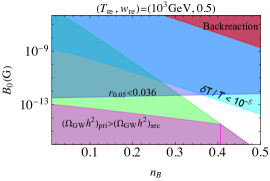
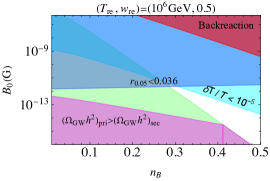
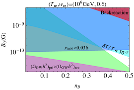
Figure 1: We have illustrated the theoretical and observational constraints in the $(B_{0},n_{\mbox{\tiny{B}}})$-plane for three sets of the parameters $(T_{\mathrm{re}},w_{\mathrm{re}})$. The different shaded regions in the figure correspond to the following: (i) forbidden due to backreaction during inflation (in red), (ii) secondary GWs induced by the PMFs after inflation surpass the Planck upper bound on the tensor-to-scalar ratio (in blue), (iii) large CMB temperature fluctuations induced by the PMFs (in cyan), (iv) the dimensionless spectral density of the primary GWs today dominates that of the secondary GWs, regardless of the frequency (in magenta), and (v) at the end of inflation the spectral density of primary GWs dominates that of the secondary GWs (in light green). We shall focus our investigation in and near the domain (v).

During reheating, the scale factor evolves as $a(\eta)=a_{\mathrm{e}}\,(\eta/\eta_{\mathrm{e}})^{\delta/2}$, where $\delta={4}/{(1+3w_{\mathrm{re}})}$. Upon using Eq. (7), the spectrum of secondary GWs at the end of reheating can be expressed as

$$\mathcal{P}^{\lambda}_{\mbox{\tiny{SEC}}}(k,\eta_{\mathrm{re}}) =\frac{2H_{\mbox{\tiny{I}}}^{4}}{M_{\mbox{\tiny{Pl}}}^{4}}\left(\frac{a_{\mathrm{e}}^{2}\mathcal{B}}{k_{\mathrm{e}}^{2}}\right)^{4}\left(\frac{k}{k_{\mathrm{e}}}\right)^{2(\delta+n_{\mbox{\tiny{B}}}-2)}\,\mathcal{F}_{n_{\mbox{\tiny{B}}}}(k)$$

$$\times[\mathcal{C}_{\mathrm{m}}^{\mathrm{re}}(x_{\mathrm{re}},x_{\mathrm{e}})]^{2},$$ (10)

where, for convenience, we have introduced the dimensionless variable $x=k\eta$, and the quantity $\mathcal{C}_{\mathrm{m}}^{\mathrm{re}}(x_{\mathrm{re}},x_{\mathrm{e}})$ is given by

$$\mathcal{C}_{\mathrm{m}}^{\mathrm{re}}(x_{\mathrm{re}},x_{\mathrm{e}})=k\,\int_{x_{\mathrm{e}}}^{x_{\mathrm{re}}}{\mathrm{d}}x_{1}x_{1}^{-\delta}G^{\rm re}_{k}(x_{\mathrm{re}},x_{1})$$ (11)

with $G^{\mathrm{re}}_{k}(x_{\mathrm{re}},x_{1})$ being the Green’s function for GWs during reheating. The tensor power spectrum at the time of the neutrino decoupling can be arrived at in a similar fashion, upon utilizing the Green’s function during the epoch of radiation domination and carrying out the integral from the conformal time $\eta_{\mathrm{re}}$ to $\eta_{\nu}$.

Since the wave numbers of our interest will be well within the Hubble radius by the late stages of the radiation-dominated epoch, the subsequent evolution of the energy density of GWs mirrors the behavior of the energy density of radiation Lewis (2004b). The total, dimensionless spectral density of primary and secondary GWs today (i.e. at $\eta_{0}$) is defined as

$$\Omega_{\mbox{\tiny{GW}}}(k)=\Omega_{\mbox{\tiny{GW}}}^{\mbox{\tiny{PRI}}}(k,\eta_{0})+\Omega_{\mbox{\tiny{GW}}}^{\mbox{\tiny{SEC}}}(k,\eta_{0})=\frac{\rho_{\mbox{\tiny{GW}}}(k,\eta_{0})}{3H_{0}^{2}M_{\mbox{\tiny{Pl}}}^{2}},$$ (12)

where $H_{0}$ denotes the present value of the Hubble parameter. If we assume inflation of the de-Sitter form, the spectral density of the primary GWs today can be expressed as (in this context, see, for instance, Ref. Haque et al. (2021a))

$$\Omega_{\mbox{\tiny{GW}}}^{\mbox{\tiny{PRI}}}(k)h^{2} \simeq 1.13\times 10^{-17}\left(\frac{H_{\mbox{\tiny{I}}}}{10^{-5}M_{\mbox{\tiny{Pl}}}}\right)^{2}$$

$$\times\left\{\begin{array}[]{ll}1&\mbox{for\leavevmode\nobreak\ }k<k_{\mathrm{re}},\\ \mathcal{D}_{1}\left(k/k_{\mathrm{re}}\right)^{-n_{w}}&\mbox{for\leavevmode\nobreak\ }k>k_{\mathrm{re}},\end{array}\right.$$ (15)

where $\mathcal{D}_{1}\simeq\mathcal{O}(1)$ and $n_{w}=2(1-3w_{\mathrm{re}})/(1+3w_{\mathrm{re}})$. With the spectrum of secondary GWs at the time of decoupling of neutrinos at hand, we find that the corresponding spectral density of GWs today can be written as follows:

$$\Omega_{\mbox{\tiny{GW}}}^{\mbox{\tiny{SEC}}}(k)h^{2}\simeq 7.17\times 10^{-26}\left(\frac{g_{0}}{g_{\mathrm{re}}}\right)^{1/3}\left(\frac{\Omega_{\mathrm{r}}h^{2}}{4.3\times 10^{-5}}\right)$$

$$\times\left(\frac{H_{\mbox{\tiny{I}}}}{10^{-5}M_{\mbox{\tiny{Pl}}}}\right)^{4}\left(\frac{\mathcal{B}a_{\mathrm{e}}^{2}}{k_{\mathrm{e}}^{2}}\right)^{4}\left(\frac{k_{\mathrm{re}}}{k_{\mathrm{e}}}\right)^{2(n_{w}+n_{\mbox{\tiny{B}}})}\mathcal{F}_{n_{\mbox{\tiny{B}}}}(k)$$ (16)

$$\times\left\{\begin{array}[]{ll}\!\!\!\mathcal{A}_{1}(k/k_{\mathrm{re}})^{2n_{\mbox{\tiny{B}}}}&\!\!\mbox{for\leavevmode\nobreak\ }k_{*}<k<k_{\mbox{\tiny{SB1}}},\\ \!\!\!\mathcal{I}_{2}(k)(k_{\mathrm{re}}/k_{\nu})^{2}(k/k_{\mathrm{re}})^{2n_{\mbox{\tiny{B}}}+2}&\!\!\mbox{for\leavevmode\nobreak\ }k_{\mbox{\tiny{SB1}}}<k<k_{\nu},\\ \!\!\!\mathcal{I}_{2}(k)(k/k_{\mathrm{re}})^{2n_{\mbox{\tiny{B}}}}&\!\!\mbox{for\leavevmode\nobreak\ }k_{\nu}<k<k_{\mathrm{re}},\\ \!\!\!\mathcal{A}_{2}(k/k_{\mathrm{re}})^{2n_{\mbox{\tiny{B}}}-|n_{w}|}&\!\!\mbox{for\leavevmode\nobreak\ }k>k_{\mathrm{re}},w_{\mathrm{re}}>1/3,\\ \!\!\!\mathcal{A}_{3}(k/k_{\mathrm{re}})^{2n_{\mbox{\tiny{B}}}-|n_{w}|}&\!\!\mbox{for\leavevmode\nobreak\ }k>k_{\mathrm{re}},w_{\mathrm{re}}<1/3,\end{array}\right.$$ (22)

where $\Omega_{\mathrm{r}}$ represents the dimensionless energy density of radiation, while $g_{\mathrm{re}}=106.75$ and $g_{0}=3.35$ represent the effective number of relativistic degrees of freedom at the end of reheating and the present day. Also, note that the quantities $(\mathcal{A}_{1},\mathcal{A}_{2},\mathcal{A}_{3})$ are listed in the supplementary material, while $\mathcal{I}_{2}(k)=[\gamma+\ln(k/k_{\mathrm{re}})]^{2}$. Moreover, $k_{\nu}$ denotes the wave number that renters the Hubble radius at the time of decoupling of the neutrinos, and we shall comment on $k_{\mbox{\tiny{SB1}}}$ below. If we demand that $\Omega_{\mbox{\tiny{GW}}}^{\mbox{\tiny{PRI}}}(k)>\Omega_{\mbox{\tiny{GW}}}^{\mbox{\tiny{SEC}}}(k)$, then upon using the expressions (15) and (16) for the dimensionless spectral densities of primary and secondary GWs at the wave number $k_{\mathrm{re}}$, we obtain the following upper bound on the strength of the PMFs:

$$\mathcal{B}\leq\frac{0.47(k_{\mathrm{e}}/a_{\mathrm{e}})^{2}}{[\mathcal{A}_{1}\mathcal{F}_{n_{\mbox{\tiny{B}}}}(k_{\mathrm{re}})]^{1/4}}\left(\frac{H_{\mbox{\tiny{I}}}}{M_{\mbox{\tiny{Pl}}}}\right)^{-1/2}\left(\frac{k_{\mathrm{e}}}{k_{\mathrm{re}}}\right)^{(n_{w}+n_{\mbox{\tiny{B}}})/2}.$$ (23)

For a given $w_{\mathrm{re}}$ and $T_{\mathrm{re}}$, this translates to a constraint on the strength $B_{0}$ and $n_{\mbox{\tiny{B}}}$ of the magnetic field today, which corresponds to the region shaded in magenta in Fig. 1.

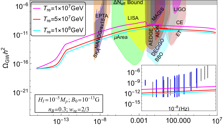
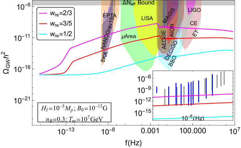
Figure 2: The combined dimensionless spectral energy density $\Omega_{\mbox{\tiny{GW}}}(k)h^{2}$ of primary and secondary gravitational GWs today have been plotted as a function of frequency $f$. Assuming a fixed magnetic field strength $B_{0}$ and spectral index $n_{\mbox{\tiny{B}}}$, we have plotted the results for different reheating temperatures $T_{\mathrm{re}}$ (on the top) and the EoS $w_{\mathrm{re}}$ (at the bottom). In the figure, we have also included the sensitivity curves of different GW observatories as well as the recent constraints from the PTA. These plots reveal that, for certain parameter ranges, the GW amplitudes are consistent with the strengths of the stochastic GW background indicated by the PTAs.

Results: As mentioned, we shall focus on situations wherein the effects due to reheating and PMFs are dominant. This corresponds to the region highlighted in light green in Fig. 1. In Fig. 2, we have plotted the total, dimensionless spectral density of GWs for a set of parameters from the domain of interest. The spectral density is characterized by a broken power law, with five distinct regions. We find that the first spectral break (SB) appears around $k_{\mbox{\tiny{SB1}}}=\mathcal{A}_{1}^{1/2}k_{\nu}/\ln(k_{\mathrm{re}}/k_{\nu})\simeq 10^{-1}k_{\nu}$. The second break arises at roughly the scale of $k_{\nu}$ and, subsequently, the third spectral break becomes apparent around $k_{\mathrm{re}}$.For $w_{\mathrm{re}}>1/3$, when $n_{\mbox{\tiny{B}}}<|n_{w}|/2$ for high frequencies, , for very high frequencies, a fourth SB occurs at $k=k_{\mbox{\tiny{SB2}}}$, beyond which the primary GWs dominate and behave as $\Omega_{\mbox{\tiny{GW}}}^{\mbox{\tiny{PRI}}}(k)\propto(k/k_{\mathrm{re}})^{|n_{w}|}$. However, we do not discuss such a case, because, for such a low $n_{\mbox{\tiny{B}}}$, we find that the spectral density of GWs does not prove to be consistent with the PTA signal. Nevertheless, the location of the second SB can be determined by comparing the primary and secondary spectral densities, and it is given by

$$\left(\frac{k_{\mbox{\tiny{SB2}}}}{k_{\mathrm{re}}}\right)^{2(|n_{w}|-n_{\mbox{\tiny{B}}})} \simeq 2.5\times 10^{-9}\left(\frac{H_{\mbox{\tiny{I}}}}{10^{-5}M_{\mbox{\tiny{Pl}}}}\right)^{2}\left(\frac{\mathcal{B}a_{\mathrm{e}}^{2}}{k_{\mathrm{e}}^{2}}\right)^{4}$$

$$\;\times\mathcal{A}_{2}\mathcal{F}_{n_{\mbox{\tiny{B}}}}(k_{\mbox{\tiny{SB2}}})\left(\frac{k_{\mathrm{re}}}{k_{\mathrm{e}}}\right)^{2(n_{w}+n_{\mbox{\tiny{B}}})}.$$ (24)

In the figure, we have also included the sensitivity curves of the different GW observatories Abbott et al. (2016, 2017); Sathyaprakash et al. (2012); Baker et al. (2019); Suemasa et al. (2017); Amaro-Seoane et al. (2013); Barausse et al. (2020); Janssen et al. (2015); Agazie et al. (2023); et al (2023); Reardon et al. (2023); Xu et al. (2023) as well as the recent data from the PTAs et al (2023). It is clear that, for a set of parameter values, the GWs generated in the scenarios we have considered are consistent with the PTA data.

Let us now assume that, at the CMB pivot scale $k_{\ast}$, the current spectral density of GWs arises solely due to the primary contributions generated during inflation. In such a case, the value of $r=0.036$ translates to $\Omega_{\mbox{\tiny{GW}}}(k_{\ast})h^{2}\simeq 10^{-17}$. Such an assumption imposes an upper limit on the contemporary magnetic field at the scale of $1\,\mathrm{Mpc}$, denoted as $B^{\mathrm{max}}_{0}$. The expression for $B_{0}^{\mathrm{max}}$ can be obtained to be

$$B_{0}^{\mathrm{max}} \simeq\frac{149(4.5)^{n_{\mbox{\tiny{B}}}}k_{\mathrm{e}}^{2}}{(\mathcal{A}_{1}\mathcal{F}_{n_{\mbox{\tiny{B}}}}(k_{*}))^{1/4}}\left(\frac{H_{\mbox{\tiny{I}}}}{10^{-5}M_{\mbox{\tiny{Pl}}}}\right)^{-1/2}\left(\frac{k_{\mathrm{e}}}{k_{\mathrm{re}}}\right)^{n_{w}/2}.$$ (25)

It is worth noting that $B^{\mathrm{max}}_{0}$ exhibits limited sensitivity to the spectral index of the magnetic field $n_{\mbox{\tiny{B}}}$. However, its dependence on $w_{\mathrm{re}}$ and $T_{\mathrm{re}}$ is significant, particularly when $w_{\mathrm{re}}\gtrsim 1/3$. These relationships are illustrated in Fig. 3, wherein we have plotted $B^{\mathrm{max}}_{0}$ as a function of $w_{\mathrm{re}}$ for two distinct values of $n_{\mbox{\tiny{B}}}$.

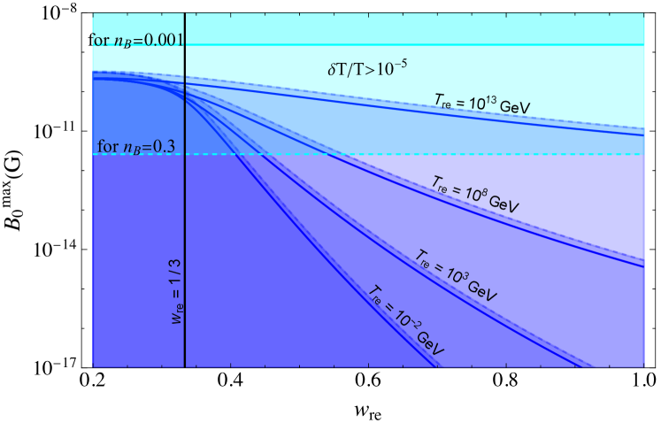
Figure 3: This figure illustrates the domains in the $(B^{\mathrm{max}}_{0},w_{\mathrm{re}})$-plane which are consistent with the constraints from the CMB on large scales for different values of $n_{\mbox{\tiny{B}}}$ and $T_{\mathrm{re}}$. While the horizontal cyan lines indicate the upper bound associated with the constraint (3), the solid and dashed blue lines indicate upper limits corresponding to the constraint (25) for $n_{\mbox{\tiny{B}}}=0.001$ and $0.3$, respectively.

Bound on $\Delta N_{\mathrm{eff}}$: Over $k>k_{\mbox{\tiny{SB2}}}$, the spectral density of primary GWs dominates the secondary ones. In this domain, the spectral index $n_{w}$ is essentially determined by the EoS during reheating [cf. Eq. (15)]. For $w_{\mathrm{re}}>1/3$, since the spectral energy density of GWs increases with frequency, the limit on the effective number of relativistic degrees of freedom, viz. $\Delta N_{\mathrm{eff}}$ provides an additional constraint. This constraint is given by Caprini and Figueroa (2018)

$$\frac{8}{7}\left(\frac{11}{4}\right)^{4/3}\frac{1}{\Omega_{\gamma}h^{2}}\int_{k_{0}}^{k_{\mathrm{e}}}\frac{{\mathrm{d}}k}{k}\Omega_{\mbox{\tiny{GW}}}(k)h^{2}\leq\Delta N_{\mathrm{eff}},$$ (26)

where $\Omega_{\gamma}h^{2}\simeq 2.47\times 10^{-5}$ represents the present-day dimensionless density of photons Aghanim et al. (2020). At the level of $2$-$\sigma$, the latest Planck 2018 + BAO data indicate that $\Delta N_{\mathrm{eff}}=0.284$ Aghanim et al. (2020). This bound leads to the inequality Clarke et al. (2020)

$$\Omega_{\mbox{\tiny{GW}}}h^{2}\simeq\frac{\Omega_{\mbox{\tiny{GW}}}(k_{\mathrm{e}})h^{2}}{|n_{w}|}\leq 1.6\times 10^{-6}\left(\frac{\Delta N_{\mathrm{eff}}}{0.284}\right).$$ (27)

which serves as an effective means to constrain the dynamics of reheating. In Tab. 1, we have listed the lower limits on the reheating temperature $T_{\mathrm{re}}$ that are consistent with the above bound for specific values of the EoS parameter $w_{\mathrm{re}}$.

$w_{\mathrm{re}}$	$3/5$	$2/3$	$5/7$	$3/4$	$7/9$	$5/6$
$T_{\mathrm{re}}^{\mathrm{min}}$ (GeV)	$20$	$6\times 10^{3}$	$10^{5}$	$10^{6}$	$3.5\times 10^{6}$	$3.3\times 10^{7}$

Table 1: The minimum reheating temperature $T_{\mathrm{re}}^{\rm min}$, corresponding to a particular EoS parameter $w_{\mathrm{re}}$, that is consistent with the constraint on $\Delta N_{\mathrm{eff}}$ [cf. Eq. (27)].

Comparing with the PTA data: Over the wave numbers $k_{\nu}<k<k_{\mathrm{re}}$, it is the magnetic spectral index $n_{\mbox{\tiny{B}}}$ that determines the slope of the spectral density of GWs [cf. Eq. (16)]. We find that suitable values of $n_{\mbox{\tiny{B}}}$ lead to GWs of strengths as observed by the PTAs in the $\mathrm{nHz}$ range of frequencies (see Fig. 2). In the analysis of the PTA data, the characteristic spectrum of the strain is assumed to be of the form $h_{\mathrm{c}}(f)=A_{\mbox{\tiny{CP}}}(f/f_{\mathrm{yr}})^{(3-\gamma_{\mbox{\tiny{CP}}})/2}$, which translates to the following spectral density of GWs: $\Omega_{\mbox{\tiny{GW}}}(f)=\Omega_{\mbox{\tiny{GW}}}^{\mathrm{yr}}(f/f_{\mathrm{yr}})^{5-\gamma_{\mbox{\tiny{CP}}}}$, where $\Omega_{\mbox{\tiny{GW}}}^{\mathrm{yr}}=2\pi^{2}f_{\mathrm{yr}}^{2}A_{\mbox{\tiny{CP}}}^{2}/(3H_{0}^{2})$. Note that $A_{\mbox{\tiny{CP}}}$ is the amplitude at the reference frequency of $f_{\mathrm{yr}}=1\mathrm{yr}^{-1}$ and $\gamma_{\mbox{\tiny{CP}}}$ is the so-called timing residual cross-power spectral index. In Fig. 4, we have illustrated the allowed region in the $(\gamma_{\mbox{\tiny{CP}}},A_{\mbox{\tiny{CP}}})$-plane from the PTA data. Over the constraints, we have superimposed the results we obtain for $A_{\mbox{\tiny{CP}}}$ and $\gamma_{\mbox{\tiny{CP}}}$ from the expression (16) for the spectral density of secondary GWs. In plotting the results, we have assumed that $B_{0}=10^{-13}\,\mathrm{G}$ and $w_{\mathrm{re}}=2/3$, and we have considered different reheating temperatures. The quantity $A_{\mbox{\tiny{CP}}}$ is approximately given by $A_{\mbox{\tiny{CP}}}\simeq 3.99\times 10^{-11}[\Omega_{\mbox{\tiny{GW}}}(f_{\mathrm{yr}})h^{2}]^{1/2}$. For the values of $B_{0}$ and $w_{\mathrm{re}}$ we have worked with, the index $\gamma_{\mbox{\tiny{CP}}}$ is determined to be $\gamma_{\mbox{\tiny{CP}}}=5-2n_{\mbox{\tiny{B}}}+\vartheta$, where $\vartheta=0.2^{+0.10}_{-0.07}$ and the uncertainty arises due to the additional dependence of $\gamma_{\mbox{\tiny{CP}}}$ on $n_{\mbox{\tiny{B}}}$. We find that, for $w_{\mathrm{re}}=2/3$ and $T_{\mathrm{re}}=10^{7}\leavevmode\nobreak\ \mathrm{GeV}$, the optimal range for $n_{\mbox{\tiny{B}}}$ is $0.37<n_{\mbox{\tiny{B}}}<0.39$. Our results appear as straight lines in the figure for different values of the reheating temperature and they are consistent with the PTA data at the confidence level of $3$-$\sigma$.

We should add that these values also satisfy the constraint on $\Delta N_{\mathrm{eff}}$ we discussed above as well as the LIGO-Virgo-Kagra bound on $\Omega_{\mbox{\tiny{GW}}}(f)$ at the reference frequency of $25\,\mathrm{Hz}$ Abbott et al. (2021).

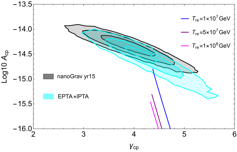
Figure 4: We have illustrated the constraints (at the levels of $1$, $2$, and $3$-$\sigma$ from the PTA data in the $(\gamma_{\mbox{\tiny{CP}}},A_{\mbox{\tiny{CP}}})$-plane. The predictions from the secondary GWs generated by the PMFs are illustrated as straight lines for $0.1<n_{\mbox{\tiny{B}}}<0.39$. Assuming $B_{0}=10^{-13}\,\mathrm{G}$ and $w_{\mathrm{re}}=2/3$, we have plotted the lines for three different values of the reheating temperatures. We find that our predictions are consistent with the PTA data at $3$-$\sigma$.

Conclusions: Arriving at strong constraints on the epoch of reheating can help us gain insight into the physics beyond the standard models of cosmology and particle physics. In this work, we have examined the impact of PMFs and reheating on secondary GWs. When $w_{\mathrm{re}}>1/3$, as has been shown earlier, the spectral density of primary GWs $\Omega_{\mbox{\tiny{GW}}}^{\mbox{\tiny{PRI}}}(f)$ has a blue tilt over wave numbers that re-enter the Hubble radius during reheating, which leads to constraints on the reheating parameters $(w_{\mathrm{re}},T_{\mathrm{re}})$ due to $\Delta N_{\mathrm{eff}}$. We have shown that, in the intermediate range of wave numbers, the spectral the density of secondary GWs induced by the PMFs can surpass the strengths of the primary GWs. We find that the combined spectra have a broken power-law form with five different indices. Importantly, for a range of parameters, the combined spectral density of GWs has strengths comparable to the stochastic GW background observed by the PTAs as well as the sensitivities of upcoming observatories. Observing these signatures could reveal the mechanisms of primordial magnetogenesis and reheating. In this work, we have not considered the case wherein, at the end of inflation, the strength of the secondary GWs is higher than the primary ones. In such a situation, the domain $w_{\mathrm{re}}<1/3$ can be accessible and we plan to consider it in a future study.

Acknowledgments: SM wishes to thank the Council of Scientific and Industrial Research, Ministry of Science and Technology, Government of India (GoI), for financial assistance. DM and LS gratefully acknowledge the support received from the Science and Engineering Research Board, Department of Science and Technology, GoI, through the Core Research Grant CRG/2020/003664. We wish to thank the Gravitation and High Energy Physics Groups at IIT Guwahati for illuminating discussions.

I Supplementary material

In this supplementary material, we shall provide a few additional details and calculations to support the discussions in the main text.

I.1 Arriving at the reheating temperature

During the reheating phase described by the EoS parameter $w_{\mathrm{re}}$, the energy density of the inflaton $\rho_{\phi}$ evolves as $\rho_{\phi}=\rho_{\mathrm{e}}\,(a/a_{\mathrm{e}})^{-3(1+w_{\mathrm{re}})}$, where $\rho_{\mathrm{e}}$ and $a_{\mathrm{e}}$ represent the energy density and scale factor at the end of inflation. In slow roll inflation driven by a single scalar field, we have $\rho_{\mathrm{e}}\simeq 3H_{\mbox{\tiny{I}}}^{2}M_{\mbox{\tiny{Pl}}}^{2}$, where $H_{\mbox{\tiny{I}}}$ denotes the nearly constant Hubble parameter. The reheating temperature $T_{\mathrm{re}}$ is defined as the temperature of radiation at the end of the epoch of reheating when the energy density of the inflaton and radiation become equal, i.e. $\rho_{\phi}(a_{\mathrm{re}})=\rho_{\mathrm{r}}(a_{\mathrm{re}})$, where $a_{\mathrm{re}}$ represents the scale factor at the end of reheating. Since the energy density of radiation is given by $\rho_{\mathrm{r}}=\pi^{2}g_{\ast}T^{4}/30$, where $g_{\ast}$ denotes the number of relativistic degrees of freedom, the reheating temperature can be obtained to be

$$T_{\mathrm{re}}=\left(\frac{90H_{\mbox{\tiny{I}}}^{2}M_{\mbox{\tiny{Pl}}}^{2}}{\pi^{2}g_{*}}\right)^{1/4}\exp\left[-\frac{3}{4}(1+w_{\mathrm{re}})N_{\mathrm{re}}\right].$$ (28)

I.2 Evolution of the EMFs during reheating

It is well known that electromagnetic fields are generated during inflation by breaking the conformal invariance of the electromagnetic action (see, for instance, Refs. Subramanian (2016); Kobayashi (2014); Haque et al. (2021b); Tripathy et al. (2022)). As we had mentioned, we shall assume that the conformal symmetry is restored at the end of inflation. If we assume that the electrical conductivity of the universe during reheating is negligible, both the electric and magnetic fields persist through this period. Then, it can be shown that, post inflation, the comoving power spectra of the electric and magnetic fields, viz. $\mathcal{P}_{\mbox{\tiny{E}}}^{\mathrm{c}}$ and $\mathcal{P}_{\mbox{\tiny{B}}}^{\mathrm{c}}$, satisfy the equations

$${\mathcal{P}_{\mbox{\tiny{E}}}^{\mathrm{c}}}^{\prime}+{\mathcal{P}_{\mbox{\tiny{B}}}^{\mathrm{c}}}^{\prime} =0,$$ (29a)

$${\mathcal{P}_{\mbox{\tiny{B}}}^{\mathrm{c}}}^{\prime\prime}+2k^{2}(\mathcal{P}_{\mbox{\tiny{B}}}^{\mathrm{c}}-\mathcal{P}_{\mbox{\tiny{E}}}^{\mathrm{c}}) =0.$$ (29b)

These coupled equations admit the following exact analytical solutions:

$$\mathcal{P}_{\mbox{\tiny{B}}}^{\mathrm{c}}(k,\eta) =\frac{a_{\mathrm{e}}^{4}}{2}\biggl{\{}\mathcal{P}_{\mbox{\tiny{B}}}^{\mbox{\tiny{I}}}(k)+\mathcal{P}_{\mbox{\tiny{E}}}^{\mbox{\tiny{I}}}(k)$$

$$\quad+[\mathcal{P}_{\mbox{\tiny{B}}}^{\mbox{\tiny{I}}}(k)-\mathcal{P}_{\mbox{\tiny{E}}}^{\mbox{\tiny{I}}}(k)]\cos[2k(\eta-\eta_{\mathrm{e}})]\biggr{\}},$$ (30a)

$$\mathcal{P}_{\mbox{\tiny{E}}}^{\mathrm{c}}(k,\eta) =\frac{a_{\mathrm{e}}^{4}}{2}\biggl{\{}\mathcal{P}_{\mbox{\tiny{B}}}^{\mbox{\tiny{I}}}(k)+\mathcal{P}_{\mbox{\tiny{E}}}^{\mbox{\tiny{I}}}(k)$$

$$\quad-[\mathcal{P}_{\mbox{\tiny{B}}}^{\mbox{\tiny{I}}}(k)-\mathcal{P}_{\mbox{\tiny{E}}}^{\mbox{\tiny{I}}}(k)]\cos[2k(\eta-\eta_{\mathrm{e}})]\biggr{\}},$$ (30b)

where $\mathcal{P}_{\mbox{\tiny{E}}}^{\mbox{\tiny{I}}}(k)$ and $\mathcal{P}_{\mbox{\tiny{B}}}^{\mbox{\tiny{I}}}(k)$ are the spectra of the electric and magnetic fields at the end of inflation. When $\mathcal{P}_{\mbox{\tiny{E}}}^{\mbox{\tiny{I}}}(k)>\mathcal{P}_{\mbox{\tiny{B}}}^{\mbox{\tiny{I}}}(k)$, on super-Hubble scales such that $k\eta\ll 1$, the above solutions simplify to

$$\mathcal{P}_{\mbox{\tiny{B}}}^{\mathrm{c}}(k,\eta) \simeq a_{\mathrm{e}}^{4}[\mathcal{P}_{\mbox{\tiny{B}}}^{\mbox{\tiny{I}}}(k)+\mathcal{P}_{\mbox{\tiny{E}}}^{\mbox{\tiny{I}}}(k)k^{2}(\eta-\eta_{\mathrm{e}})^{2}],$$ (31a)

$$\mathcal{P}_{\mbox{\tiny{E}}}^{\mathrm{c}}(k,\eta) \simeq a_{\mathrm{e}}^{4}\mathcal{P}_{\mbox{\tiny{E}}}^{\mbox{\tiny{I}}}(k).$$ (31b)

Therefore, during reheating, the power spectra of the electromagnetic fields evolve as

$$\mathcal{P}_{\mbox{\tiny{B}}}(k,\eta) \simeq\left(\frac{a_{\mathrm{e}}}{a}\right)^{4}\left[\mathcal{P}_{\mbox{\tiny{B}}}^{\mbox{\tiny{I}}}(k)+\mathcal{P}_{\mbox{\tiny{E}}}^{\mbox{\tiny{I}}}(k)\gamma^{2}(k)\left(\frac{a_{\mathrm{e}}H_{\mbox{\tiny{I}}}}{aH}-1\right)^{2}\right]$$ (32a)

$$\mathcal{P}_{\mbox{\tiny{E}}}(k,\eta) \simeq\left(\frac{a_{\mathrm{e}}}{a}\right)^{4}\mathcal{P}_{\mbox{\tiny{E}}}^{\mbox{\tiny{I}}}(k)$$ (32b)

where $\gamma(k)=2(k/k_{\mathrm{e}})/(1+3w_{\mathrm{re}})$ and, to arrive at the expression for $\mathcal{P}_{\mbox{\tiny{B}}}(k,\eta)$, we have used the relation Haque et al. (2021b)

$$k^{2}(\eta-\eta_{\mathrm{e}})^{2}\simeq\left(\frac{2}{1+3w_{\mathrm{re}}}\right)^{2}\left(\frac{k}{k_{\mathrm{e}}}\right)^{2}\left(\frac{a_{\mathrm{e}}H_{\mbox{\tiny{I}}}}{aH}-1\right)^{2}.$$ (33)

I.3 Calculation of $(a_{\mathrm{e}}/a_{0})$ from entropy conservation

To arrive at the strength of the magnetic fields today, we need the ratio of the scale factors at the end of reheating and today, i.e. $a_{\mathrm{re}}$ and $a_{0}$. This can be arrived at by demanding that the entropy of the universe is conserved after reheating. Using the conservation of entropy, it can shown that reheating temperature $T_{\mathrm{re}}$ and the present-day temperature of the CMB $T_{\gamma 0}$ and the neutrino background $T_{\nu 0}$ can be expressed as

$$g_{*}T_{\mathrm{re}}^{3}=\left(\frac{a_{0}}{a_{\mathrm{re}}}\right)^{3}\left(2T_{\gamma 0}^{3}+\frac{21}{4}T_{\nu 0}^{3}\right).$$ (34)

Also, since $T_{\nu 0}=(4/11)^{1/3}T_{0}$, we obtain that

$$\frac{a_{\mathrm{re}}}{a_{0}}=\left(\frac{43}{11g_{*}}\right)^{1/3}\frac{T_{\gamma 0}}{T_{\mathrm{re}}}.$$ (35)

which, in turn, leads to

$$\frac{a_{\mathrm{e}}}{a_{0}}=\frac{a_{\mathrm{e}}}{a_{\mathrm{re}}}\frac{a_{\mathrm{re}}}{a_{0}}=\left(\frac{43}{11g_{*}}\right)^{1/3}\mathrm{e}^{-N_{\mathrm{re}}}\frac{T_{\gamma 0}}{T_{\mathrm{re}}}.$$ (36)

I.4 Calculation of $\mbox{B}_{0}^{\mathrm{max}}$ from the fluctuations in the the temperature of the CMB

Recall that the energy density of radiation is given by $\rho_{r}=g_{\ast}\pi^{2}T^{4}/30$. Hence, the dimensionless ratio of the fluctuation in the energy density can be expressed as

$$\frac{\delta\rho_{r}}{\rho_{r}}=4\frac{\delta T}{T}.$$ (37)

This quantity remains conserved throughout the epoch of radiation domination since both the fluctuations and the background evolve as $a^{-4}$. However, it is not conserved during the epoch of reheating era. The background energy density evolves as $a^{-3(1+w_{\mathrm{re}})}$ during this period. However, the fluctuations in the energy density, mainly from arising in the energy density of electromagnetic radiation, evolve as $a^{-4}$. If we assume that all the fluctuations arose from the fluctuations in the the energy density of electromagnetic radiation, we can express $\delta\rho/\rho$ at the end of the reheating era as follows:

$$\left.\frac{\delta\rho}{\rho}\right|_{a_{\mathrm{re}}}=\frac{\rho_{\mathrm{em}}^{\mathrm{I}}}{\rho_{\mathrm{e}}}\left(\frac{a_{e}}{a_{\text{re}}}\right)^{1-3w_{\text{re}}}.$$ (38)

For simplicity, if we neglect the effects after the phase of reheating, we can connect the fluctuations in the temperature of the CMB today to the above quantity as

$$\frac{\rho_{\mathrm{em}}^{\mathrm{I}}}{\rho_{\mathrm{e}}}\left(\frac{a_{\mathrm{e}}}{a_{\mathrm{re}}}\right)^{1-3w_{\mathrm{re}}}=4\left.\frac{\delta T}{T}\right|_{\mathrm{CMB}},$$ (39)

where $\rho_{\mathrm{em}}^{\mathrm{I}}$ represents the total electromagnetic energy density at the end of inflation. The quantity $\rho_{\mathrm{em}}^{\mathrm{I}}$ is given by

$$\rho_{\mathrm{em}}^{\mathrm{I}}=\int_{k_{\mathrm{min}}}^{k_{\mathrm{e}}}\frac{{\mathrm{d}}k}{k}\mathcal{P}_{\mbox{\tiny{B}}}^{\mbox{\tiny{I}}}(k)=\frac{\mathcal{B}^{2}}{n_{\mbox{\tiny{B}}}}\left[1-\left(\frac{k_{\mathrm{min}}}{k_{\mathrm{e}}}\right)^{n_{\mbox{\tiny{B}}}}\right],$$ (40)

where we have assumed that the power spectrum of the magnetic field is dominant during inflation and $k_{\mathrm{min}}$ is the wave number corresponding to the largest scale observable today.

Observations of the CMB constrain the fluctuations in the temperature to be $\delta T/T\sim 10^{-5}$. To avoid a significant impact on the fluctuations in the temperature of the CMB, the perturbation in the energy density of radiation must be small. Upon using this condition, we obtain that

$$\mathcal{B}^{2}=\frac{12n_{\mbox{\tiny{B}}}H_{\mbox{\tiny{I}}}^{2}M_{\mbox{\tiny{Pl}}}^{2}}{1-(k_{\mathrm{min}}/k_{\mathrm{e}})^{n_{\mbox{\tiny{B}}}}}\left(\frac{a_{\mathrm{re}}}{a_{\mathrm{e}}}\right)^{1-3w_{\mathrm{re}}}\left.\frac{\delta T}{T}\right|_{\text{CMB}},$$ (41)

which leads to

$$\mathcal{B}^{2} \simeq 12\times 10^{-15}M_{\mbox{\tiny{Pl}}}^{4}\left(\frac{H_{\mbox{\tiny{I}}}}{10^{-5}M_{\mbox{\tiny{Pl}}}}\right)^{2}f_{n_{\mbox{\tiny{B}}}}$$

$$\quad\times\left(\frac{a_{\mathrm{re}}}{a_{\mathrm{e}}}\right)^{1-3w_{\mathrm{re}}}\times\left(\frac{\delta T/T}{10^{-5}}\right)_{\text{CMB}},$$ (42)

where $f_{n_{\mbox{\tiny{B}}}}=n_{\mbox{\tiny{B}}}/[1-(k_{\mathrm{min}}/k_{\mathrm{e}})^{n_{\mbox{\tiny{B}}}}]$.

From the definition (1a) of the power spectrum of the magnetic field, the strength of the magnetic field today at the roughly CMB scale of $1\,\mathrm{Mpc}$ can be written as

$$B_{0}^{\mbox{\tiny{{CMB}}}}=\mathcal{B}\left(\frac{a_{\mathrm{e}}}{a_{0}}\right)^{2}\left(\frac{1\,\mathrm{Mpc}^{-1}}{k_{\mathrm{e}}}\right)^{n_{\mbox{\tiny{B}}}/2}.$$ (43)

Further, upon using Eqs. (41) and (36), we arrive at

$$B_{0}^{\mbox{\tiny{{CMB}}}} \simeq 1.17\times 10^{-8}\left(\frac{H_{\mbox{\tiny{I}}}}{10^{-5}M_{\mbox{\tiny{Pl}}}}\right)$$

$$\quad\times f_{n_{\mbox{\tiny{B}}}}^{1/2}\left(\frac{1\,\mathrm{Mpc}^{-1}}{k_{\mathrm{e}}}\right)^{n_{\mbox{\tiny{B}}}/2}\mathrm{G}.$$ (44)

For a scale-invariant spectrum of the primordial magnetic field, the bound from fluctuations in the temperature of the CMB turn out to be approximately $B_{0}^{\mbox{\tiny{{CMB}}}}\simeq 1.55$ nG, which is the result we have quoted in the text.

I.5 Constraints due to backreaction during inflation

The production of electromagnetic fields during inflation can modify the Friedmann equation if the energy density of the electromagnetic the field becomes comparable to that of the background energy density that drives inflation. Therefore, it is crucial to ensure that the energy density of the electromagnetic fields that are generated during inflation are less than the energy density of the inflaton. Recall that the energy density of the scalar field at the end of inflation can be expressed as $\rho(\eta_{\mathrm{e}})\simeq 3H_{\mbox{\tiny{I}}}^{2}M_{\mbox{\tiny{Pl}}}^{2}$. If we now assume that the magnetic fields with spectra $\mathcal{P}_{\mbox{\tiny{B}}}^{\mbox{\tiny{I}}}=\mathcal{B}^{2}(k/k_{\mathrm{e}})^{n_{\mbox{\tiny{B}}}}$ dominate the energy density, then, to avoid the issue of backreaction, we find that the quantity $\mathcal{B}$ is subject to the constraint

$$\mathcal{B}^{2}\lesssim 3H_{\mbox{\tiny{I}}}^{2}M_{\mbox{\tiny{Pl}}}^{2}f_{n_{\mbox{\tiny{B}}}}.$$ (45)

This constraint translates to the following constraint on the strength of the magnetic field today [cf. Eq. (43)]:

$$B_{0}^{\text{b}}\lesssim 5.25\times 10^{51}\,\left(\frac{H_{\mbox{\tiny{I}}}}{10^{-5}M_{\mbox{\tiny{Pl}}}}\right)f_{n_{\mbox{\tiny{B}}}}^{1/2}\left(\frac{a_{\mathrm{e}}}{a_{0}}\right)^{2}\mathrm{G}.$$ (46)

In the case of instantaneous reheating, upon using the expression for $(a_{0}/a_{\mathrm{e}})$ in Eq. (36), we obtain that

$$B_{0,\text{max}}^{\text{b}}\lesssim 1.85\times 10^{-6}\,\left(\frac{H_{\mbox{\tiny{I}}}}{10^{-5}M_{\mbox{\tiny{Pl}}}}\right)f_{n_{\mbox{\tiny{B}}}}^{1/2}\mathrm{G}.$$ (47)

I.6 Spectral density of secondary GWs generated during inflation

In this subsection, we aim to determine the limits on the strength of the present-day magnetic field under the condition that the spectral energy the density of the secondary GWs evaluated at the end of inflation [viz. $\Omega_{\mbox{\tiny{GW}}}^{\mbox{\tiny{SEC}}}(k,\eta_{\mathrm{e}})$] is lower than the corresponding spectral density of primary GWs [i.e. $\Omega_{\mbox{\tiny{GW}}}^{\mbox{\tiny{PRI}}}(k,\eta_{\mathrm{e}})$]. To arrive at the constraint we need to compute the spectral density of GWs generated during inflation, which, in turn, requires knowledge of the evolution of the electromagnetic modes during inflation.

Following the widely accepted models of magnetogenesis Subramanian (2016); Kobayashi (2014); Haque et al. (2021b); Tripathy et al. (2022); Sorbo (2011); Caprini and Sorbo (2014); Ito and Soda (2017), we shall assume that, towards the end of inflation, the spectrum of the magnetic field is of the form $\mathcal{P}_{\mbox{\tiny{B}}}(k,\eta)=\mathcal{B}^{2}(-k\eta)^{n_{\mbox{\tiny{B}}}}$. Moreover, we shall assume that the strengths of the electric field are considerably weaker. For simplicity, if we further assume that the background during inflation is of the de-Sitter form, then the Green’s function associated with the tensor perturbations at late times is given by $G_{k}^{\mathrm{inf}}(\eta,\eta_{1})\simeq\eta_{1}/3$ Caprini and Sorbo (2014). Upon substituting these forms for the Green’s function and the behavior of the electromagnetic modes into Eq. (7), we obtain the tensor power spectrum at the end of inflation to be Caprini and Sorbo (2014)

$$\mathcal{P}^{\lambda,\mathrm{inf}}_{\mbox{\tiny{SEC}}}(k,\eta_{\mathrm{e}}) =\frac{2\mathcal{B}^{4}}{M_{\mbox{\tiny{Pl}}}^{4}}\int_{k_{\mathrm{min}}}^{k_{\mathrm{e}}}\frac{{\mathrm{d}}q}{q}\int_{-1}^{1}{\mathrm{d}}\mu\frac{(q/k)^{n_{\mbox{\tiny{B}}}}f(\mu,\beta)}{\left[1+(q/k)^{2}-2\mu(q/k)\right]^{(3-n_{\mbox{\tiny{B}}})/2}}\left[\int_{\eta_{i}}^{\eta_{\mathrm{e}}}{\mathrm{d}}\eta_{1}a^{2}(\eta_{1})G_{k}^{\mathrm{inf}}(\eta_{\mathrm{e}},\eta_{1})(k\eta_{1})^{n_{\mbox{\tiny{B}}}}\right]^{2}$$

$$=\frac{2\mathcal{B}^{4}}{M_{\mbox{\tiny{Pl}}}^{4}}\int_{k_{\mathrm{min}}}^{k_{\mathrm{e}}}\frac{{\mathrm{d}}q}{q}\int_{-1}^{1}{\mathrm{d}}\mu\frac{(q/k)^{n_{\mbox{\tiny{B}}}}f(\mu,\beta)}{\left[1+(q/k)^{2}-2\mu(q/k)\right]^{(3-n_{\mbox{\tiny{B}}})/2}}\left[\int_{x_{i}}^{x_{\mathrm{e}}}\frac{{\mathrm{d}}x_{1}}{3}x_{1}^{n_{\mbox{\tiny{B}}}-1}\right]^{2}$$

$$=\frac{2H_{\mbox{\tiny{I}}}^{4}}{M_{\mbox{\tiny{Pl}}}^{4}}\left(\frac{\mathcal{B}}{H_{\mbox{\tiny{I}}}^{2}}\right)^{4}\mathcal{I}_{\rm inf}^{2}(k)\mathcal{F}_{n_{\mbox{\tiny{B}}}}(k),$$ (48)

where we have set $x_{1}=k\eta_{1}$ and the quantities $\mathcal{F}_{n_{\mbox{\tiny{B}}}}(k)$ and $\mathcal{I}_{\mathrm{inf}}(k)$ are given by

$$\mathcal{F}_{n_{\mbox{\tiny{B}}}}(k) =\int_{k_{\mathrm{min}}}^{k_{\mathrm{e}}}\frac{{\mathrm{d}}q}{q}\int_{-1}^{1}{\mathrm{d}}\mu\frac{(q/k)^{n_{\mbox{\tiny{B}}}}f(\mu,\beta)}{\left[1+(q/k)^{2}-2\mu(q/k)\right]^{(3-n_{\mbox{\tiny{B}}})/2}}\simeq\frac{16}{3n_{\mbox{\tiny{B}}}}\left[1-\left(\frac{k_{\mathrm{min}}}{k}\right)^{n_{\mbox{\tiny{B}}}}\right]+\frac{2\alpha}{3}\left[\left(\frac{k_{\mathrm{e}}}{k}\right)^{2n_{\mbox{\tiny{B}}}-3}-1\right]$$ (49)

$$\mathcal{I}_{\mathrm{inf}}(k) =\frac{1}{3n_{\mbox{\tiny{B}}}}\left[\left(\frac{k}{k_{\mathrm{e}}}\right)^{n_{\mbox{\tiny{B}}}}-\left(\frac{k}{k_{*}}\right)^{n_{\mbox{\tiny{B}}}}\right]$$ (50)

with $\alpha=56/[5(2n_{\mbox{\tiny{B}}}-3)]$.

In contrast, the tensor power spectrum of the primary GWs originating from the vacuum fluctuations during inflation are given by

$$\mathcal{P}^{\lambda,\mathrm{inf}}_{\mbox{\tiny{PRI}}}(k,\eta_{\mathrm{e}})=\frac{2}{\pi^{2}}\left(\frac{H_{\mbox{\tiny{I}}}}{M_{\mbox{\tiny{Pl}}}}\right)^{2}\,\left(1+\frac{k^{2}}{k_{\mathrm{e}}^{2}}\right)$$ (51)

Our objective is to compute the minimum strength of the magnetic field that ensures the dominance of the primary tensor power spectrum over the secondary one. Note that we shall be interested in situations wherein the spectrum of the magnetic field has a slight blue tilt. In such a case, the spectrum of secondary GWs has the maximum strength at $k=k_{\mathrm{e}}$. Therefore, upon equating the expressions (48) and (51) for the spectra of the primary and secondary GWs at the wavenumber $k_{\mathrm{e}}$, we obtain the following condition on the amplitude $\mathcal{B}$ of the inflationary

$$\mathcal{B} =\frac{2H_{\mbox{\tiny{I}}}^{2}}{\pi^{2}}\left(\frac{M_{\mbox{\tiny{Pl}}}}{H_{\mbox{\tiny{I}}}}\right)^{1/2}\frac{1}{[\mathrm{I}_{n_{\mbox{\tiny{B}}}}(k_{\mathrm{e}})\mathcal{F}_{n_{\mbox{\tiny{B}}}}(k_{\mathrm{e}})]^{1/4}}\simeq 0.202\left(\frac{M_{\mbox{\tiny{Pl}}}}{H_{\mbox{\tiny{I}}}}\right)^{1/2}\frac{H_{\mbox{\tiny{I}}}^{2}}{[\mathrm{I}_{n_{\rm B}}(k_{\mathrm{e}})\mathcal{F}_{n_{\mbox{\tiny{B}}}}(k_{\mathrm{e}})]^{1/4}},$$ (52)

where $\mathrm{I}_{n_{\mbox{\tiny{B}}}}(k_{\mathrm{e}})=[1-(k_{\mathrm{e}}/k_{*})^{n_{\mbox{\tiny{B}}}}]^{2}/(9n_{\mbox{\tiny{B}}}^{2})$.

I.7 Post-inflationary contributions to the secondary tensor power spectrum

The electromagnetic fields are expected to have been generated during inflation due to a non-conformal coupling. We shall assume that the conformal symmetry of the electromagnetic action is restored at the end of inflation. As a result, the electromagnetic modes simply oscillate post-inflation, apart from the diluting factor that arises due to the expansion of the universe. The tensor modes ${h_{\bm{k}}^{\lambda}}$ are governed by the equation (see, for instance, Ref. Caprini and Sorbo (2014))

$${h_{\bm{k}}^{\lambda}}^{\prime\prime}+2\mathcal{H}{h_{\bm{k}}^{\lambda}}^{\prime}+k^{2}{h_{\bm{k}}^{\lambda}}=\mathcal{S}_{\bm{k}},$$ (53)

where the source term $\mathcal{S}_{\bm{k}}(\eta)$ is given by

$$\mathcal{S}_{\bm{k}}(\eta)=-\frac{2}{M_{\mbox{\tiny{Pl}}}^{2}a^{2}}\Pi^{\lambda}_{lm}({\bm{k}})\int\frac{{\mathrm{d}}^{3}{\bm{q}}}{(2\pi)^{3/2}}\left[{A}^{\prime}_{l}({\bm{q}},\eta){A}^{\prime}_{m}({\bm{k}}-{\bm{q}},\eta)-\epsilon_{lab}q_{a}{A}_{b}({\bm{q}},\eta)\epsilon_{mcd}({\bm{k}}-{\bm{q}})_{c}{A}_{d}({\bm{k}}-{\bm{q}},\eta)\right].$$ (54)

The Green’s function corresponding to Eq. (53) satisfies the differential equation

$$G_{k}^{\prime\prime}(\eta,\eta_{1})+2\mathcal{H}G_{k}^{\prime}(\eta,\eta_{1})+k^{2}G_{k}(\eta,\eta_{1})=\delta^{(1)}(\eta-\eta_{1}).$$ (55)

The Green’s function during the epochs of reheating and radiation domination can be easily obtained to be

$$G_{k}^{\mathrm{re}}(\eta,\eta_{1}) =\theta(\eta-\eta_{1})\frac{\pi\eta^{l}\eta_{1}^{1-l}}{2\mathrm{sin}(l\pi)}\left[J_{l}(k\eta)J_{-l}(k\eta_{1})-J_{-l}(k\eta)J_{l}(k\eta_{1})\right],$$ (56a)

$$G_{k}^{\mathrm{ra}}(\eta,\eta_{1}) =\theta(\eta-\eta_{1})\frac{\eta_{1}}{k\eta}\sin[k(\eta_{1}-\eta)],$$ (56b)

where $l=(1-\delta)/2$ with $\delta=4/(1+3w_{\mathrm{re}})$.

Evidently, at the time of neutrino decoupling $\eta_{\nu}$, the tensor perturbations generated by the magnetic fields can be expressed

$${h_{\bm{k}}^{\lambda}}(\eta_{\nu})=\int_{\eta_{\mathrm{e}}}^{\eta_{\mathrm{re}}}{\mathrm{d}}\eta_{1}G_{k}^{\mathrm{re}}(\eta_{\mathrm{re}},\eta_{1})\mathcal{S}_{\bm{k}}(\eta_{1})+\int_{\eta_{\mathrm{re}}}^{\eta_{\nu}}{\mathrm{d}}\eta_{1}G_{k}^{\mathrm{ra}}(\eta_{\nu},\eta_{1})\mathcal{S}_{\bm{k}}(\eta_{1}).$$ (57)

Since we have assumed that the electric fields are sub-dominant post-inflation, we find that the tensor power spectrum [as defined in Eq. (7)] can be expressed as

$$\mathcal{P}^{\lambda}_{\mbox{\tiny{SEC}}}(k,\eta_{\nu}) =\frac{2a_{\mathrm{e}}^{8}}{M_{\mbox{\tiny{Pl}}}^{4}}\left[\int_{\eta_{\mathrm{e}}}^{\eta_{\mathrm{re}}}\frac{{\mathrm{d}}\eta_{1}}{a^{2}(\eta_{1})}G_{k}^{\mathrm{re}}(\eta_{\mathrm{re}},\eta_{1})+\int_{\eta_{\mathrm{re}}}^{\eta_{\nu}}\frac{d\eta_{1}}{a^{2}(\eta_{1})}G_{k}^{\mathrm{ra}}(\eta_{\nu},\eta_{1})\right]^{2}\int_{0}^{\infty}\frac{{\mathrm{d}}q}{q}\int_{-1}^{1}\frac{{\mathrm{d}}\mu f(\mu,\beta)\mathcal{P}_{\mbox{\tiny{B}}}^{\mbox{\tiny{I}}}(q)\mathcal{P}_{\mbox{\tiny{B}}}^{\mbox{\tiny{I}}}(|\bm{k}-\bm{q}|)}{[1+\left(q/k\right)^{2}-2\mu(q/k)]^{3/2}}$$

$$=\frac{2a_{\mathrm{e}}^{8}}{M_{\mbox{\tiny{Pl}}}^{4}k^{4}}\left[\mathcal{C}_{\rm re}(x_{\mathrm{re}},x_{\mathrm{e}})+\mathcal{C}_{\rm ra}(x_{\nu},x_{\mathrm{re}})\right]^{2}\int_{0}^{\infty}\frac{{\mathrm{d}}q}{q}\int_{-1}^{1}\frac{{\mathrm{d}}\mu f(\mu,\beta)\mathcal{P}_{\mbox{\tiny{B}}}^{\mbox{\tiny{I}}}(q)\mathcal{P}_{\mbox{\tiny{B}}}^{\mbox{\tiny{I}}}(|\bm{k}-\bm{q}|)}{[1+\left(q/k\right)^{2}-2\mu(q/k)]^{3/2}}$$

$$\simeq\frac{2a_{\mathrm{e}}^{8}}{M_{\mbox{\tiny{Pl}}}^{4}k^{4}}\left[\mathcal{C}_{\rm re}^{2}(x_{\mathrm{re}},x_{\mathrm{e}})+\mathcal{C}_{\rm ra}^{2}(x_{\nu},x_{\mathrm{re}})\right]\int_{0}^{\infty}\frac{{\mathrm{d}}q}{q}\int_{-1}^{1}\frac{{\mathrm{d}}\mu f(\mu,\beta)\mathcal{P}_{\mbox{\tiny{B}}}^{\mbox{\tiny{I}}}(q)\mathcal{P}_{\mbox{\tiny{B}}}^{\mbox{\tiny{I}}}(|\bm{k}-\bm{q}|)}{[1+\left(q/k\right)^{2}-2\mu(q/k)]^{3/2}},$$ (58)

where we have set $x=k\eta$, and the quantities $\mathcal{C}_{\rm re}(x_{\mathrm{e}},x_{\mathrm{re}})$ and $\mathcal{C}_{\rm re}(x_{\mathrm{e}},x_{\nu})$ are given by

$$\mathcal{C}_{\rm re}(x_{\mathrm{re}},x_{\mathrm{e}}) =k\,\int_{x_{\mathrm{e}}}^{x_{\mathrm{re}}}\frac{{\mathrm{d}}x_{1}}{a^{2}(x_{1})}G_{k}^{\mathrm{re}}(x_{\mathrm{re}},x_{1})=\frac{kx_{\mathrm{e}}^{\delta}}{a_{\mathrm{e}}^{2}}\int_{x_{\mathrm{e}}}^{x_{\mathrm{re}}}{\mathrm{d}}x_{1}x_{1}^{-\delta}G_{k}^{\mathrm{re}}(x_{\mathrm{re}},x_{1})=\frac{x_{\mathrm{e}}^{\delta}}{a_{\mathrm{e}}^{2}}\mathcal{C}_{\mathrm{m}}^{\mathrm{re}}(x_{\mathrm{re}},x_{\mathrm{e}}),$$ (59a)

$$\mathcal{C}_{\rm ra}(x_{\nu},x_{\mathrm{re}}) =k\,\int_{x_{\mathrm{re}}}^{x_{\nu}}\frac{{\mathrm{d}}x_{1}}{a^{2}(x_{1})}G_{k}^{\mathrm{ra}}(x_{\nu},x_{1})=\frac{kx_{\mathrm{re}}^{2}}{a_{\mathrm{re}}^{2}}\int_{x_{\mathrm{re}}}^{x_{\nu}}{\mathrm{d}}x_{1}x_{1}^{-2}G_{k}^{\mathrm{ra}}(x_{\nu},x_{1})=\frac{x_{\mathrm{re}}^{2}}{a_{\mathrm{re}}^{2}}\mathcal{C}_{\rm r}^{\rm ra}(x_{\nu},x_{\mathrm{re}}).$$ (59b)

In arriving at the final expressions above, we have made use of the following forms of the scale factor during the epochs of reheating and radiation domination:

$$a(\eta)=\left\{\begin{array}[]{ll}a_{\mathrm{e}}(x/x_{\mathrm{e}})^{\delta/2}&\mathrm{for}\leavevmode\nobreak\ \eta_{\mathrm{e}}\leq\eta\leq\eta_{\mathrm{re}},\\ a_{\mathrm{re}}(x/x_{\mathrm{re}})&\mathrm{for}\leavevmode\nobreak\ \eta_{\mathrm{re}}\leq\eta\leq\eta_{\mathrm{eq}},\end{array}\right.$$ (62)

where $\eta_{\mathrm{eq}}$ represents the conformal time corresponding to the epoch of radiation-matter equality.

I.7.1 Calculating $\mathcal{C}_{\rm re}(x_{\mathrm{re}},x_{\mathrm{e}})$ and $\mathcal{C}_{\rm re}(x_{\nu},x_{\mathrm{re}})$

Let us now compute the quantities $\mathcal{C}_{\rm re}(x_{\mathrm{e}},x_{\mathrm{re}})$ and $\mathcal{C}_{\rm re}(x_{\mathrm{re}},x_{\nu})$ during the epochs of reheating and radiation domination. During reheating, upon using the functional form (56a) for the Green’s function, the indefinite integral in Eq. (59a) can be evaluated to be

$$\mathcal{C}_{\mathrm{m}}^{\mathrm{re}}(x,x_{1}) =k\int{\mathrm{d}}x_{1}x_{1}^{-\delta}G_{k}^{\mathrm{re}}(x,x_{1})=\frac{\pi x^{l}}{2\mathrm{sin}(l\pi)}\int{\mathrm{d}}x_{1}x_{1}^{1-l-\delta}\left[J_{l}(x)J_{-l}(x_{1})-J_{-l}(x)J_{l}(x_{1})\right]$$

$$=2^{-2-l}x^{l}x_{1}^{2-2l-\delta}\biggl{\{}\frac{\Gamma(-l)\Gamma[1-(\delta/2)]}{\Gamma[2-(\delta/2)]}x_{1}^{2l}J_{-l}(x)\,{}_{1}F_{2}[1-(\delta/2);1+l,2-(\delta/2);-(x_{1}^{2}/4)]$$

$$+4^{l}\frac{\Gamma(l)\Gamma[1-l-(\delta/2)]}{\Gamma[2-l-(\delta/2)]}J_{l}(x){}_{1}F_{2}[1-l-(\delta/2);1-l,2-l-(\delta/2);-(x_{1}^{2}/4)]\biggr{\}},$$ (63)

where ${}_{1}F_{2}(a,b,c,z)$ denotes the hypergeometric function. Similarly, upon substituting the Green’s function (56b) during the radiation dominated epoch in Eq. (59b) and carrying out the integral, we obtain that

$$\mathcal{C}_{\rm r}^{\rm ra}(x_{\nu},x_{\mathrm{re}}) =k\int_{x_{\mathrm{re}}}^{x_{\nu}}{\mathrm{d}}x_{1}x_{1}^{-2}G_{k}^{\mathrm{ra}}(x_{\nu},x_{1})=\frac{1}{x_{\nu}}\int_{x_{\mathrm{re}}}^{x_{\nu}}\frac{{\mathrm{d}}x_{1}}{x_{1}}\sin(x_{\nu}-x_{1})=\frac{1}{x_{\nu}}\mathcal{I}(x_{\nu},x_{\mathrm{re}})$$ (64)

For convenience, we break the above integral into two regions i.e. $k<k_{\nu}$ and $k_{\nu}<k<k_{\mathrm{re}}$. In these cases, the integral $\mathcal{I}(x_{\nu},x_{\mathrm{re}})$ reduces to

$$\mathcal{I}(x_{\nu},x_{\mathrm{re}})\simeq\left\{\begin{array}[]{ll}\left[\gamma_{\mathrm{E}}+\ln\left(k/k_{\mathrm{re}}\right)\right](k/k_{\nu})&\mbox{for\leavevmode\nobreak\ }k<k_{\nu},\\ \gamma_{\mathrm{E}}+\ln\left(k/k_{\mathrm{re}}\right)&\mbox{for\leavevmode\nobreak\ }k_{\nu}<k<k_{\mathrm{re}},\end{array}\right.$$ (67)

where $\gamma_{\mathrm{E}}=0.577$ is the Euler’s constant.

I.7.2 Contributions to the secondary tensor power spectrum

At the end of reheating, the secondary tensor power spectrum induced by the magnetic fields can be expressed as

$$\mathcal{P}^{\lambda,\mathrm{re}}_{\mbox{\tiny{SEC}}}(k,\eta_{\mathrm{re}}) =\frac{2a_{\mathrm{e}}^{8}}{M_{\mbox{\tiny{Pl}}}^{4}k^{4}}\left[\mathcal{C}_{\mathrm{m}}^{\mathrm{re}}(x_{\mathrm{e}},x_{\mathrm{re}})\right]^{2}\int_{0}^{\infty}\frac{{\mathrm{d}}q}{q}\int_{-1}^{1}\frac{{\mathrm{d}}\mu f(\mu,\beta)\mathcal{P}_{\mbox{\tiny{B}}}^{\mbox{\tiny{I}}}(q)\mathcal{P}_{\mbox{\tiny{B}}}^{\mbox{\tiny{I}}}(|\bm{k}-\bm{q}|}{[1+\left(q/k\right)^{2}-2\mu(q/k)]^{3/2}}$$

$$=\frac{2k_{\mathrm{e}}^{8}}{M_{\mbox{\tiny{Pl}}}^{4}k^{4}a_{\mathrm{e}}^{4}}\left(\frac{a_{\mathrm{e}}^{2}\mathcal{B}}{k_{\mathrm{e}}^{2}}\right)^{4}\left(\frac{k}{k_{\mathrm{e}}}\right)^{2(\delta+n_{\mbox{\tiny{B}}})}\left[{\mathcal{C}_{\mathrm{m}}^{\mathrm{re}}}(x_{\mathrm{e}},x_{\mathrm{re}})\right]^{2}\int_{0}^{\infty}\frac{dq}{q}\int_{-1}^{1}{\mathrm{d}}\mu\frac{f(\mu,\beta)(q/k)^{n_{\mbox{\tiny{B}}}}}{\left[(1+(q/k)^{2}-2\mu(q/k)\right]^{(3-n_{\mbox{\tiny{B}}})/2}}$$

$$=\frac{2H_{\mbox{\tiny{I}}}^{4}}{M_{\mbox{\tiny{Pl}}}^{4}}\left(\frac{a_{\mathrm{e}}^{2}\mathcal{B}}{k_{\mathrm{e}}^{2}}\right)^{4}\left(\frac{k}{k_{\mathrm{e}}}\right)^{2(\delta+n_{\mbox{\tiny{B}}}-2)}\left[\mathcal{C}_{\mathrm{m}}^{\mathrm{re}}(x_{\mathrm{e}},x_{\mathrm{re}})\right]^{2}\mathcal{F}_{n_{\mbox{\tiny{B}}}}(k),$$ (68)

where $\mathcal{F}_{n_{\mbox{\tiny{B}}}}(k)$ is given by Eq. (49). In a similar fashion, the contribution to the secondary tensor power spectrum due to the magnetic fields during the epoch of radiation domination can be expressed as

$$\mathcal{P}^{\lambda,\mathrm{ra}}_{\mbox{\tiny{SEC}}}(k,\eta_{\nu}) =\frac{2a_{\mathrm{e}}^{8}}{M_{\mbox{\tiny{Pl}}}^{4}k^{4}}\frac{x_{\mathrm{re}}^{4}}{a_{\mathrm{re}}^{4}}\left[\mathcal{C}_{\rm r}^{\rm ra}(x_{\mathrm{re}},x_{\nu})\right]^{2}\int_{0}^{\infty}\frac{{\mathrm{d}}q}{q}\int_{-1}^{1}\frac{{\mathrm{d}}\mu f(\mu,\beta)\mathcal{P}_{\mbox{\tiny{B}}}^{\mbox{\tiny{I}}}(q)\mathcal{P}_{\mbox{\tiny{B}}}^{\mbox{\tiny{I}}}(|\bm{k}-\bm{q}|}{[1+\left(q/k\right)^{2}-2\mu(q/k)]^{3/2}}$$

$$=\frac{2k_{\mathrm{e}}^{8}x_{\mathrm{re}}^{4}}{M_{\mbox{\tiny{Pl}}}^{4}k^{4}a_{\mathrm{e}}^{4}}\left(\frac{a_{\mathrm{e}}}{a_{\mathrm{re}}}\right)^{4}\left(\frac{a_{\mathrm{e}}^{2}\mathcal{B}}{k_{\mathrm{e}}^{2}}\right)^{4}\left(\frac{k}{k_{\mathrm{e}}}\right)^{2n_{\mbox{\tiny{B}}}}\left[\mathcal{C}_{\rm r}^{\rm ra}(x_{\mathrm{re}},x_{\nu})\right]^{2}\mathcal{F}_{n_{\mbox{\tiny{B}}}}(k)$$

$$=\frac{2H_{\mbox{\tiny{I}}}^{4}}{M_{\mbox{\tiny{Pl}}}^{4}}\left(\frac{x_{\mathrm{re}}}{x_{\mathrm{e}}}\right)^{4}\left(\frac{a_{\mathrm{e}}}{a_{\mathrm{re}}}\right)^{4}\left(\frac{a_{\mathrm{e}}^{2}\mathcal{B}}{k_{\mathrm{e}}^{2}}\right)^{4}\left(\frac{k}{k_{\mathrm{e}}}\right)^{2n_{\mbox{\tiny{B}}}}\left[\mathcal{C}_{\rm r}^{\rm ra}(x_{\mathrm{re}},x_{\nu})\right]^{2}\mathcal{F}_{n_{\mbox{\tiny{B}}}}(k)$$

$$=\frac{2H_{\mbox{\tiny{I}}}^{4}}{M_{\mbox{\tiny{Pl}}}^{4}}\left(\frac{a_{\mathrm{e}}^{2}\mathcal{B}}{k_{\mathrm{e}}^{2}}\right)^{4}\mathrm{e}^{2(3w_{\mathrm{re}}-1)N_{\mathrm{re}}}\left(\frac{k}{k_{\mathrm{e}}}\right)^{2n_{\mbox{\tiny{B}}}}\left[\mathcal{C}_{\rm r}^{\rm ra}(x_{\mathrm{re}},x_{\nu})\right]^{2}\mathcal{F}_{n_{\mbox{\tiny{B}}}}(k).$$ (69)

Lastly, the contribution due to cross-term in the secondary tensor power spectrum can be expressed as

$$\mathcal{P}_{\rm T,s}^{\rm c}(k) =\frac{4a_{\mathrm{e}}^{8}}{M_{\mbox{\tiny{Pl}}}^{4}k^{4}}\mathcal{C}_{\rm re}(x_{\mathrm{e}},x_{\mathrm{re}})\,\mathcal{C}_{\rm ra}(x_{\mathrm{re}},x_{\nu})\int_{0}^{\infty}\frac{{\mathrm{d}}q}{q}\int_{-1}^{1}\frac{{\mathrm{d}}\mu f(\mu,\beta)\mathcal{P}_{\mbox{\tiny{B}}}^{\mbox{\tiny{I}}}(q)\mathcal{P}_{\mbox{\tiny{B}}}^{\mbox{\tiny{I}}}(|\bm{k}-\bm{q}|}{[1+\left(q/k\right)^{2}-2\mu(q/k)]^{3/2}}$$

$$=\frac{4k_{\mathrm{e}}^{8}}{M_{\mbox{\tiny{Pl}}}^{4}k^{4}}\left(\frac{a_{\mathrm{e}}^{2}\mathcal{B}}{k_{\mathrm{e}}^{2}}\right)^{4}\frac{x_{\mathrm{e}}^{\delta}}{a_{\mathrm{e}}^{2}}\frac{x_{\mathrm{re}}^{2}}{a_{\mathrm{re}}^{2}}\mathcal{C}_{\mathrm{m}}^{\mathrm{re}}(x_{\mathrm{e}},x_{\mathrm{re}})\,\mathcal{C}_{\rm r}^{\rm ra}(x_{\mathrm{re}},x_{\nu})\left(\frac{k}{k_{\mathrm{e}}}\right)^{2n_{\mbox{\tiny{B}}}}\mathcal{F}_{n_{\mbox{\tiny{B}}}}(k)$$

$$=\frac{4H_{\mbox{\tiny{I}}}^{4}}{M_{\mbox{\tiny{Pl}}}^{4}}\left(\frac{a_{\mathrm{e}}^{2}\mathcal{B}}{k_{\mathrm{e}}^{2}}\right)^{4}\left(\frac{a_{\mathrm{e}}}{a_{\mathrm{re}}}\right)^{2}\left(\frac{k}{k_{\mathrm{e}}}\right)^{2n_{\mbox{\tiny{B}}}+\delta-2}\mathcal{C}_{\mathrm{m}}^{\mathrm{re}}(x_{\mathrm{e}},x_{\mathrm{re}})\,\mathcal{C}_{\rm r}^{\rm ra}(x_{\mathrm{re}},x_{\nu})\mathcal{F}_{n_{\mbox{\tiny{B}}}}(k)$$

$$=\frac{4H_{\mbox{\tiny{I}}}^{4}}{M_{\mbox{\tiny{Pl}}}^{4}}\left(\frac{a_{\mathrm{e}}^{2}\mathcal{B}}{k_{\mathrm{e}}^{2}}\right)^{4}\mathrm{e}^{(3w_{\mathrm{re}}-1)\,N_{\mathrm{re}}}\left(\frac{k}{k_{\mathrm{e}}}\right)^{2n_{\mbox{\tiny{B}}}+\delta-2}\mathcal{C}_{\mathrm{m}}^{\mathrm{re}}(x_{\mathrm{e}},x_{\mathrm{re}})\,\mathcal{C}_{\rm r}^{\rm ra}(x_{\mathrm{re}},x_{\nu})\mathcal{F}_{n_{\mbox{\tiny{B}}}}(k).$$ (70)

We find that this cross-term is subdominant compared to the other two terms [i.e. those given by Eqs. (68) and (69)]. It is for this reason that, in Eq. (58), we have dropped this term in the final expression for the secondary tensor power spectrum.

I.7.3 Spectral shape of $\Omega_{\mbox{\tiny{GW}}}(k)$ for $k<k_{\mathrm{re}}$ and $k\gg k_{\mathrm{re}}$

Over wave numbers such that $k\ll k_{\mathrm{re}}$, we can consider the limit wherein $x_{\mathrm{e}}\ll x_{\mathrm{re}}\ll 1$. In such a case, we find that the quantity $\mathcal{C}_{\mathrm{m}}^{\mathrm{re}}(x_{\mathrm{re}},x_{\mathrm{e}})$ simplifies to be

$$\lim_{k\ll k_{\mathrm{re}}}\mathcal{C}_{\mathrm{m}}^{\mathrm{re}}(x_{\mathrm{re}},x_{\mathrm{e}})\simeq\frac{1}{(1-\delta)^{2}}\left\{\frac{2}{1+2\delta}-\frac{2}{2-\delta}\left[1-\left(\frac{k_{\mathrm{re}}}{k_{\mathrm{e}}}\right)^{2-\delta}\right]\right\}\left(\frac{k}{k_{\mathrm{re}}}\right)^{2-\delta}.$$ (71)

Similarly, when $k\gg k_{\mathrm{re}}$, for $w_{\mathrm{re}}>1/3$, the quantity $\mathcal{C}_{\mathrm{m}}^{\mathrm{re}}(x_{\mathrm{re}},x_{\mathrm{e}})$ reduces to

$$\lim_{k\gg k_{\mathrm{re}}}\mathcal{C}_{\mathrm{m}}^{\mathrm{re}}(x_{\mathrm{re}},x_{\mathrm{e}}) \simeq\sqrt{\frac{2}{\pi}}\frac{2^{(1-\delta)/2}}{(1-\delta)}\Gamma[(3-\delta)/2]\Gamma[(\delta-1)/2]x_{\mathrm{re}}^{-\delta/2}\biggl{\{}\frac{\Gamma[(1-\delta)/2]}{\Gamma(\delta/2)}\cos\left[x_{\mathrm{re}}-(2-\delta)\pi/4\right]$$

$$-\frac{2}{2-\delta}\cos\left[x_{\mathrm{re}}-\delta\pi/4\right]\biggr{\}},$$ (72)

whereas, for $w_{\mathrm{re}}<1/3$, the quantity simplifies to

$$\lim_{k\gg k_{\mathrm{re}}}\mathcal{C}_{\mathrm{m}}^{\mathrm{re}}(x_{\mathrm{e}},x_{\mathrm{re}}) \simeq\sqrt{\frac{2}{\pi}}\frac{2^{(\delta-3)/2}}{(1-\delta)}\frac{\Gamma[(\delta-1)/2]\Gamma[1-(\delta/2)]}{\Gamma[2-(\delta/2)]}x_{\mathrm{re}}^{-\delta/2}x_{\mathrm{e}}^{2-\delta}\cos\left[-x_{\mathrm{re}}+\delta\pi/4\right]$$

$$\simeq\sqrt{\frac{2}{\pi}}\frac{2^{(\delta-3)/2}\Gamma[\frac{\delta-1}{2}]}{(1-\delta)(1-\delta/2)}x_{\mathrm{re}}^{-\delta/2}x_{\mathrm{e}}^{2-\delta}\cos[x_{\mathrm{re}}-(2-\delta)\pi/4]$$ (73)

At the end of reheating, the power spectrum of secondary GWs generated due to the magnetic fields [defined in Eq. (10)] is given by

$$\mathcal{P}^{\lambda,\mathrm{re}}_{\mbox{\tiny{SEC}}}(k,\eta_{\mathrm{re}})=\frac{2H_{\mbox{\tiny{I}}}^{4}}{M_{\mbox{\tiny{Pl}}}^{4}}\left(\frac{a_{\mathrm{e}}^{2}\mathcal{B}}{k_{\mathrm{e}}^{2}}\right)^{4}\left(\frac{k}{k_{\mathrm{e}}}\right)^{2(\delta+n_{\mbox{\tiny{B}}}-2)}\,\mathcal{F}_{n_{\mbox{\tiny{B}}}}(k)\,\mathcal{C}^{2}(x_{\mathrm{re}},x_{\mathrm{e}}).$$ (74)

On substituting Eq. (71) in this expression, for $k\ll k_{\mathrm{re}}$, we obtain that

$$\mathcal{P}^{\lambda,\mathrm{re}}_{\mbox{\tiny{SEC}}}(k,\eta_{\mathrm{re}})\simeq\mathcal{A}_{1}\left(\frac{\mathcal{B}a_{\mathrm{e}}^{2}}{k_{\mathrm{e}}^{2}}\right)^{4}\left(\frac{H_{\mbox{\tiny{I}}}}{M_{\mbox{\tiny{Pl}}}}\right)^{4}\left(\frac{k_{\mathrm{re}}}{k_{\mathrm{e}}}\right)^{2(\delta-2)}\left(\frac{k}{k_{\mathrm{e}}}\right)^{2n_{\mbox{\tiny{B}}}}\mathcal{F}_{n_{\mbox{\tiny{B}}}}(k).$$ (75)

Similarly, on utilizing Eqs. (I.7.3) and (I.7.3)), for $k>k_{\mathrm{re}}$, we obtain the following expressions

$$\mathcal{P}^{\lambda,\mathrm{re}}_{\mbox{\tiny{SEC}}}(k,\eta_{\mathrm{re}}) \simeq\mathcal{A}_{2}\left(\frac{\mathcal{B}a_{\mathrm{e}}^{2}}{k_{\mathrm{e}}^{2}}\right)^{4}\left(\frac{H_{\mbox{\tiny{I}}}}{M_{\mbox{\tiny{Pl}}}}\right)^{4}\left(\frac{k_{\mathrm{re}}}{k_{\mathrm{e}}}\right)^{2(\delta-2)}\left(\frac{k}{k_{\mathrm{re}}}\right)^{-2-|n_{w}|}\left(\frac{k}{k_{\mathrm{e}}}\right)^{2n_{\mbox{\tiny{B}}}}\mathcal{F}_{n_{\mbox{\tiny{B}}}}(k),$$ (76)

$$\mathcal{P}^{\lambda,\mathrm{re}}_{\mbox{\tiny{SEC}}}(k,\eta_{\mathrm{re}}) \simeq\mathcal{A}_{3}\left(\frac{\mathcal{B}a_{\mathrm{e}}^{2}}{k_{\mathrm{e}}^{2}}\right)^{4}\left(\frac{H_{\mbox{\tiny{I}}}}{M_{\mbox{\tiny{Pl}}}}\right)^{4}\left(\frac{k_{\mathrm{re}}}{k_{\mathrm{e}}}\right)^{2(\delta-2)}\left(\frac{k}{k_{\mathrm{re}}}\right)^{-2-|n_{w}|}\left(\frac{k}{k_{\mathrm{e}}}\right)^{2n_{\mbox{\tiny{B}}}}\mathcal{F}_{n_{\mbox{\tiny{B}}}}(k),$$ (77)

when $w_{\mathrm{re}}>1/3$ and $w_{\mathrm{re}}<1/3$, respectively. The quantities $\mathcal{A}_{1}$, $\mathcal{A}_{2}$ and $\mathcal{A}_{3}$ that appear in the above expressions are given by

$$\mathcal{A}_{1} =\frac{2}{(1-\delta)^{4}}\left\{\frac{2}{1+2\delta}-\frac{2}{2-\delta}\left[1-\left(\frac{k_{\mathrm{re}}}{k_{\mathrm{e}}}\right)^{2-\delta}\right]\right\}^{2},$$ (78)

$$\mathcal{A}_{2} =\frac{2^{(3-\delta)}\Gamma^{2}[(3-\delta)/2]\Gamma^{2}[(\delta-1)/2]}{\pi(1-\delta)^{2}}\biggl{\{}\frac{\Gamma[(1-\delta)/2]}{\Gamma(\delta/2)}\cos\left[(k/k_{\mathrm{re}})-(2-\delta)\pi/4\right]-\frac{2}{2-\delta}\cos\left[(k/k_{\mathrm{re}})-\delta\pi/4\right]\biggr{\}}^{2},$$ (79)

$$\mathcal{A}_{3} =\frac{2^{\delta-1}\Gamma^{2}[(\delta-1)/2]}{\pi(1-\delta)^{2}(1-\delta/2)^{2}}\left(\frac{k_{\mathrm{re}}}{k_{\mathrm{e}}}\right)^{2(2-\delta)}\cos^{2}[(k/k_{\mathrm{re}})-\delta{\pi}/{4}].$$ (80)

I.8 Constraints from the tensor-to-scalar ratio $r$

The latest results from the Planck mission lead to a stringent upper-bound on the tensor-to-scalar ratio to be $r\leq 0.036$. At the pivot scale of $k_{\ast}=0.05\,\mathrm{Mpc}^{-1}$, the bound translates to the spectral energy density of GWs to be $\Omega_{\mbox{\tiny{GW}}}(k_{\ast})h^{2}\leq 1.13\times 10^{-17}$. If we stipulate that, at this scale, the entire contribution arises from the primary GWs, then such a condition leads to further constraints on the strengths of the magnetic fields today. On utilizing the spectral density of secondary GWs we have already computed [cf. Eq. (16)] and demanding that it does not surpass the spectral the density of primary GWs at the pivot scale [cf. Eq. (15)], we obtain that

$$\mathcal{B}\left(\frac{a_{\mathrm{e}}}{a_{0}}\right)^{2} \leq\frac{149.5\,k_{\mathrm{e}}^{2}}{[\mathcal{A}_{1}\mathcal{F}_{n_{\mbox{\tiny{B}}}}(k_{\ast})]^{1/4}}\left(\frac{H_{\mbox{\tiny{I}}}}{10^{-5}M_{\mbox{\tiny{Pl}}}}\right)^{-1/2}$$

$$\quad\times\left(\frac{k_{\mathrm{e}}}{k_{\mathrm{re}}}\right)^{n_{w}/2}\left(\frac{k_{\mathrm{e}}}{k_{*}}\right)^{n_{\mbox{\tiny{B}}}/2}.$$ (81)

On further substituting Eq. (81) in Eq. (43), we obtain the corresponding strength of the present-day magnetic field strength at the scale of $1\,\mathrm{Mpc}$ to be

$$B_{0}^{\mathrm{max}}\simeq\frac{149.5\,(4.5)^{n_{\mbox{\tiny{B}}}}k_{\mathrm{e}}^{2}}{[\mathcal{A}_{1}\mathcal{F}_{n_{\mbox{\tiny{B}}}}(k_{*})]^{1/4}}\left(\frac{H_{\mbox{\tiny{I}}}}{10^{-5}M_{\mbox{\tiny{Pl}}}}\right)^{-1/2}\left(\frac{k_{\mathrm{e}}}{k_{\mathrm{re}}}\right)^{n_{w}/2}.$$ (82)

I.9 PTA data and the value of $A_{\mbox{\tiny{CP}}}$

For comparison with the PTA data, the spectrum of the characteristic strain is parametrized as $h_{\mathrm{c}}(f)=A_{\mbox{\tiny{CP}}}(f/f_{\mathrm{yr}})^{(3-\gamma_{\mbox{\tiny{CP}}})/2}$, where, evidently, $A_{\mbox{\tiny{CP}}}$ corresponds to the amplitude of the strain at the reference frequency of $f_{\mathrm{yr}}=k_{\mathrm{yr}}/(2\pi)=1\leavevmode\nobreak\ \mathrm{yr}^{-1}=3.17\times 10^{-8}\,\mathrm{Hz}$ and $\gamma_{\mbox{\tiny{CP}}}$ denotes the so-called timing residual cross-power spectral density. This characterization is then translated into the spectral density of GWs as $\Omega_{\mbox{\tiny{GW}}}(f)=\Omega_{\mbox{\tiny{GW}}}^{\mathrm{yr}}(f/f_{\mathrm{yr}})^{5-\gamma_{{\rm CP}}}$, with $\Omega_{\mbox{\tiny{GW}}}^{\mathrm{yr}}=2\pi^{2}f_{\mathrm{yr}}^{2}A_{\mbox{\tiny{CP}}}^{2}/(3H_{0}^{2})$, where $H_{0}\simeq 1.34\times 10^{-41}\leavevmode\nobreak\ \mathrm{GeV}$ represents the present-day value of the Hubble parameter. Using the above expression for $\Omega_{\mbox{\tiny{GW}}}(f)$, we can write

$$\Omega_{\mbox{\tiny{GW}}}(f_{\mathrm{yr}})h^{2}=\frac{2\pi^{2}f_{\mathrm{yr}}^{2}A_{\mbox{\tiny{CP}}}^{2}}{3(H_{0}/h)^{2}}=\frac{k_{\mathrm{yr}}^{2}A_{\mbox{\tiny{CP}}}^{2}}{6(H_{0}/h)^{2}}$$ (83)

$k_{\mathrm{yr}}=2\pi f_{\mathrm{yr}}=2.046\times 10^{7}\leavevmode\nobreak\ \text{Mpc}^{-1}=1.311\times 10^{-31}\leavevmode\nobreak\ \text{GeV}$, so that

$$A_{\mbox{\tiny{CP}}} =\frac{\sqrt{6}(H_{0}/h)}{k_{\mathrm{yr}}}[\Omega_{\mbox{\tiny{GW}}}(f_{\mathrm{yr}})h^{2}]^{1/2}$$

$$\simeq 3.99\times 10^{-11}[\Omega_{\mbox{\tiny{GW}}}(f_{\mathrm{yr}})h^{2}]^{1/2}.$$ (84)