Energy balance and damage for brittle fracture: nonlocal formulation

Robert P. Lipton Department of Mathematics, Louisiana State University, Baton Rouge, LA 70803, Orcid: https://orcid.org/0000-0002-1382-3204, lipton@lsu.edu    Debdeep Bhattacharya Department of Mathematics, University of Utah, Salt Lake City, UT 84112, Orcid: https://orcid.org/0000-0001-5171-5506, d.Bhattacharya@utah.edu
Abstract

A nonlocal model of peridynamic type for dynamic brittle damage is introduced consisting of two phases, one elastic and the other inelastic. Evolution from the elastic to the inelastic phase depends on material strength. Existence and uniqueness of the displacement-failure set pair follow from the initial value problem. The displacement-failure pair satisfies energy balance. The length scale of nonlocality $\epsilon$ is taken to be small relative to the domain in $\mathbb{R}^{d}$, $d=2,3$. The new nonlocal model delivers a two point strain dynamics on a subset of $\mathbb{R}^{d}\times\mathbb{R}^{d}$. This dynamics provides an energy that interpolates between volume energy corresponding to elastic behavior and surface energy corresponding to failure. The deformation energy resulting in material failure over a region $R$ is given by a $d-1$ dimensional integral that is uniformly bounded as $\epsilon\rightarrow 0$. For fixed $\epsilon$, this energy is nonzero for $d-1$ dimensional regions $R$ associated with flat crack surfaces. The failure energy is the Griffith fracture energy for a given crack $R$ in terms of its area for $d=3$ (or length for $d=2$). Simulations illustrate fracture evolution through generation of an internal traction free boundary as a wake left behind a moving strain concentration. Crack paths are seen to follow a maximal strain energy density criterion.

1 Introduction

Peridynamic simulations implicitly couple the evolution of damage and deformation inside a material specimen through a nonlocal formulation using force interaction between neighboring points. They provide for the spontaneous emergence and growth of fissures as part of the dynamic simulation [32, 33]. This idea has been adapted and expanded and the literature is now very large, see for example, the contributions [31, 6, 13, 1, 35, 16, 18, 15, 4, 34, 26, 10, 30], books and reviews [5, 19, 17, 8]. The time evolution of peridynamic simulations are driven by temporally and spatially nonlocal forces. What is missing so far is: 1) a complete theory for a material undergoing irreversible damage guaranteeing energy balance and 2) an explicit formula for the energy necessary for material failure and the size of a $d-1$ dimensional “fracture” set proportional to the critical energy release rate. Both of these aspects must follow directly from the evolution equation for the deformation multiplied by the velocity and integration by parts. These theoretical aspects are addressed in this article.

Here we rigorously pursue the free discontinuity problem for fracture mechanics and propose a model that demonstrably preserves energy balance to discover new advantages to the nonlocal approach. Motivated by [32], the existence theory of [11, 10, 22] and the rate form of energy balance found in [23] we introduce a new nonlocal dynamic model to show existence of displacement-failure set pairs for two and three dimensional specimens $\Omega$ made from homogeneous material. The purpose of this paper is to model brittle damage and to recover dynamic energy balance for displacement-failure set pairs.

A small deformation model for brittle failure under tensile loading is considered. Forces between pairs of points in $\Omega$ are referred to as bonds. Bond forces depend on a two-point strain. The force between pairs of points act elastically against compressive strain and for moderate tensile strain the force is linear elastic. As one continues to increases tensile strain it becomes nonlinear elastic and at a critical strain the force becomes unstable and softens with increasing strain. The force eventually goes to zero with increasing strain and the bond between points breaks. This process is irreversible and the bonds once broken do not heal. In this model the maximum length scale of nonlocal interaction is both finite and small relative to the size of the domain and is denoted by $\epsilon$. The failure set $\Gamma^{\epsilon}(t)$ is the set of pairs of points with broken bonds in $\Omega$ at time $t$, see Section 2.

This level of generalization together with Newton’s second law and the new constitutive relation implicitly couple elastic forces and failure allowing failure sets and deformation to emerge from a two point strain dynamics. In addition to existence, the model provides energy balance. The rate form of energy balance is shown to follow directly from the evolution equation for the deformation multiplied by the velocity and integration by parts. The rate form of energy balance shows that damage must start occurring when the energy input to the system exceeds the material’s ability to generate kinetic and elastic energy through displacement and velocity, see Section 4. The energy expended up to time $t$ resulting in material failure over a region $\Gamma^{\epsilon}(t)$ is given by a bounded $d-1$ dimensional geometric integral of the failure set. Application of Gronwall’s inequality shows that the geometric integral is bounded uniformly in $\epsilon$ for initial and boundary conditions that are independent of $\epsilon$.

As an example, consider the failure set $\Gamma^{\epsilon}(t)$ defined by a flat two dimensional piece of surface $R_{t}$ where points above the surface are no longer influenced by forces due to points below the surface and vice versa. This is the case of alignment, i.e., all bonds connecting points $\mathbf{y}$ above $R_{t}$ to points $\mathbf{x}$ below are broken. Calculation of the failure energy of $\Gamma^{\epsilon}(t)$ shows that it is the product of the critical energy release rate of fracture mechanics multiplied by the two dimensional surface measure of $R_{t}$, see Section 5. The surface $R_{t}$ defines an internal boundary to domain $\Omega$ and the crack is unambiguously described as the internal boundary. Displacement jumps can only occur across $R_{t}$ and traction forces are zero on either side of $R_{t}$. Additionally, the analysis of Section 5 shows that material failure is associated with a maximum energy dissipation condition on each bond.

The example given above shows that the failure energy corresponds to Griffith fracture energy for flat cracks. This demonstrates that the failure energy is bounded and nonzero on $d-1$ dimensional sets corresponding to cracks. The explicit geometry of the failure set is controlled by how it grows dynamically. Growth is governed by the rate of work done against boundary forces and the dynamic interaction between elastic displacement and bond failure. Although interaction is captured implicitly through the evolution equations, one can now apply the rate form of energy balance to explicitly deliver the time rate of the damage energy and characterize the location of the region undergoing damage. This region is called the process zone $PZ^{\epsilon}(t)$ and from the constitutive law, corresponds to the regions of highest strain. The damage rate and process zone are determined by the displacement field through the rate of work done by the load and the change in both the kinetic energy and elastic potential energy of the specimen. The rate form of energy balance also dictates the onset of crack nucleation. The rate form of balance and its ramifications are introduced in Section 4. For a flat mode-I crack in a plate the strain is greatest in a neighborhood of the tips and this the location of the process zone. We establish energy balance in terms of Griffith fracture energy under suitably defined loading, see Section 5. Numerical simulations illustrate crack propagation featuring the alignment of broken bonds behind the propagating strain concentration. Simulation clearly shows maximum strain energy dissipation [29] as a crack path selection mechanism for a bifurcating crack, see Section 9.

On the other hand, away from damaging zones, it is shown that the model delivers the energy density associated with isotropic linear elasticity. Explicit formulas for the Lamé constants in terms of the force potentials are obtained, see Section 6. In this way, it is seen that the energy for this model is given by the surface energy over failure zones and a volume energy associated with linear elastic behavior inside quiescent zones. This is also demonstrated in Section 7 for a flat crack propagating from left to right in a plate. We consider a sequence of nonlocal initial value problems for a crack propagating from left to right, parameterized by $\epsilon$, and pass to the limit of vanishing horizon to find that the limit displacement field is a solution of the linear elastic wave equation outside a propagating traction free crack. Moreover, the same elastic constants derived in Section 6 appear in the limit of vanishing horizon providing self-consistency for the model, see Section 7. In Section 8 we outline the non-dimensional parameter appearing in the dynamics. It is found that it gives the ratio between the elastic force and fracture resistance multiplied by the domain size.

We illustrate the modeling for two different bond breaking criteria developed in [11] and [10] for a related but different class of bond forces. We depart from the previous bond breaking approaches and add a $\epsilon^{-(d+1)}$ scaling to the bond force and insert a factor of $\sqrt{|\mathbf{y}-\mathbf{x}|}$ into the bond force and bond breaking criteria, see Section 2. This change produces the desired model that is linear elastic in quiescent regions away from the damage set but nonlinear elastic with larger strain in the neighborhood of bond breaking. Strikingly, the scaling allows the failure energy to be nonzero and strictly positive for flat $d-1$ dimensional failure sets corresponding to creation of internal boundaries i.e., cracks. Previous work addresses the same constitutive law treated in this paper within a discrete quasistatic model [2]. Earlier work treats the same strain versus force law but without the presence of a damage factor, that approach is done in the context of tension loading [21, 22, 24, 25].

In summary, we observe in this paper that nonlocal dynamics for displacement with bond breaking over $\Omega$ in $\mathbb{R}^{d}$ provides a dynamics for a two-point strain over a subset of $\mathbb{R}^{d}\times\mathbb{R}^{d}$. This is used to deliver a displacement-failure set pair, see Section 2. Applying this observation allows one to construct a dynamics with energy that interpolates between volume energy corresponding to elastic behavior and surface energy corresponding to failure, see Section 4.

2 A new formulation

The body containing the damaging material $\Omega$ is a bounded domain in two or three dimensions. Nonlocal interactions between a point in the body $\mathbf{x}$ and its neighbors $\mathbf{y}$ are confined to the sphere (disk) of radius $\epsilon$ denoted by $H_{\epsilon}(\mathbf{x})=\{\mathbf{y}:\,|\mathbf{y}-\mathbf{x}|<\epsilon\}$. Here $V^{\epsilon}_{d}=\omega_{d}\epsilon^{d}$ is the $d$ dimensional volume of the ball $H_{\epsilon}(\mathbf{x})$ centered at $\mathbf{x}$ where $\omega_{d}$ is the volume of the $d$ dimensional unit ball. The elastic displacement $\mathbf{u}(t,\mathbf{x})$ is defined for $0\leq t\leq T$ and $\mathbf{x}$ in $\Omega$. We write $\mathbf{u}(t)=\mathbf{u}(t,\cdot)$ and introduce the two point strain $S(\mathbf{y},\mathbf{x},\mathbf{u}(t))$ between the point $\mathbf{x}$ and any point $\mathbf{y}\in H_{\epsilon}(\mathbf{x})$ given by

$\displaystyle S(\mathbf{y},\mathbf{x},\mathbf{u}(t))=\frac{(\mathbf{u}(t,\mathbf{y})-\mathbf{u}(t,\mathbf{x}))}{|\mathbf{y}-\mathbf{x}|}\cdot\mathbf{e},$ $\displaystyle\hbox{ where }\mathbf{e}=\frac{\mathbf{y}-\mathbf{x}}{|\mathbf{y}-\mathbf{x}|},$ (2.1)

and we set

$$r:=r(t,\mathbf{u})=\sqrt{|\mathbf{y}-\mathbf{x}|}S(\mathbf{y},\mathbf{x},\mathbf{u}(t)).$$

The strain satisfies $S(\mathbf{y},\mathbf{x},\mathbf{u}(t))=S(\mathbf{x},\mathbf{y},\mathbf{u}(t))$. The scaled nonlocal kernel is introduced and is given by

$$\rho^{\epsilon}(\mathbf{y},\mathbf{x})=\frac{{\chi_{\Omega}(\mathbf{y})}J^{\epsilon}(|\mathbf{y}-\mathbf{x}|)}{\epsilon V^{\epsilon}_{d}},$$ (2.2)

where $\chi_{\Omega}$ is the characteristic function of $\Omega$, $J^{\epsilon}(|\mathbf{y}-\mathbf{x}|)$ is the influence function, a positive function on the ball of radius $\epsilon$ centered at $\mathbf{x}$ and is radially decreasing taking the value $M$ at the center of the ball and 00 for $|\mathbf{y}-\mathbf{x}|\geq\epsilon$. The radially symmetric influence function is written $J^{\epsilon}(|\mathbf{y}-\mathbf{x}|)=J(|\mathbf{y}-\mathbf{x}|/\epsilon)$. The nonlocal kernel is scaled by $\epsilon^{-1}(V_{d}^{\epsilon})^{-1}$ enabling the model to be calibrated to a given material with known shear $\mu$ and Lamé $\lambda$ moduli in the linear elastic regime and critical energy release rate $\mathcal{G}_{c}$ when the material fails. This is established in Sections 5 and 6.

Figure 1: The potential function $g(r)$ and derivatives $g^{\prime}(r)$ and $g^{\prime\prime}(r)$ for tensile force. Here $C^{+}=g_{\infty}$ and $C^{-}=g_{-\infty}$ are the asymptotic values of $g$. The derivative of the force potential goes smoothly to zero at $r^{+}$ and $r^{-}$.

Bond force is related to strain similar to the cohesive force law given in [21, 22]. Under this law, the force is linear for small positive strains and for larger positive strains the force begins to soften and becomes zero after reaching a critical strain. For negative strain, the bond force resists the strain. These features are encoded into the force function expressed in terms of the derivative of the potential function $g(r)$ defined for, $-\infty<r<\infty$, with $g(r^{-}):=g_{-\infty}$ for $r\leq r^{-}$, and $g(r^{+}):=g_{\infty}$ for $r^{+}\leq r$. We choose $r^{c}$ and $r^{e}$ such that $r^{-}<r^{c}<r^{e}<r^{+}$ and the potential is convex for $r^{e}\leq r\leq r^{c}$ and concave otherwise. Here we assume $-r^{e}$ is much larger than $r^{c}$. The force potential used here is given in Figure 1. Here, the functions $g^{\prime},\,g^{\prime\prime}$ (depicted in Figure 1) satisfy

$\displaystyle\max_{-\infty<r<\infty}\{|g^{\prime}(r)|\}<\infty$  $\displaystyle\,\hbox{ and }\max_{-\infty<r<\infty}\{|g^{\prime\prime}(r)|\}<\infty.$ (2.3)

To construct the constitutive law relating force to strain, set $r^{\pm}=\sqrt{|\mathbf{y}-\mathbf{x}|}S^{\pm}$, so that $g^{\prime}(r)=0$ for $r\leq r^{-}$ and $r^{+}\leq r$ and set $r^{c}=\sqrt{|\mathbf{y}-\mathbf{x}|}S^{c}$ and $r^{e}=\sqrt{|\mathbf{y}-\mathbf{x}|}S^{e}$. We require $g^{\prime\prime}(r)$ to be continuous on $-\infty<r<\infty$. The constitutive law relating force to strain and subsequent bond failure is given by

$$\boldsymbol{f}^{\epsilon}(t,\mathbf{y},\mathbf{x},\mathbf{u})=\frac{2\rho^{\epsilon}(\mathbf{y},\mathbf{x})}{\sqrt{|\mathbf{y}-\mathbf{x}|}}\gamma(\mathbf{u})(\mathbf{y},\mathbf{x},t)g^{\prime}(r(t,\mathbf{u}))\boldsymbol{e},$$ (2.4)

where $\gamma(\mathbf{u})(\mathbf{y},\mathbf{x},t)$ is the degradation factor that decreases from one when critical strain is reached. The first form of degradation factor is a scaled version of the one presented in [11]. Let $(r-r^{+})^{+}$ be the positive part of $r-r^{+}$ and the degradation factor $\gamma(\mathbf{u})(\mathbf{y},\mathbf{x},t)$ is given by

$\displaystyle\gamma(\mathbf{u})(\mathbf{y},\mathbf{x},t)=h\left(\int_{0}^{t}\,(\,r(\tau,\mathbf{u}))-r^{+})^{+}\,d\tau\right),$ (2.5)

$h=h(x)$ is nonnegative, takes the value one for arguments $x<0$, decreases smoothly to zero for $0\leq x<x^{D}$, and is zero for $x^{D}\leq x$, see Figure 1. It is clear from this definition that irrevocable degradation occurs when the strain exceeds $S^{+}=r^{+}/\sqrt{|\mathbf{y}-\mathbf{x}|}$ and the time spent above the threshold depends on the strain rate. The bond between $\mathbf{x}$ and $\mathbf{y}$ fails (breaks) when $\gamma(\mathbf{u})(\mathbf{y},\mathbf{x},t)=0$. The time to failure can be made small by taking $x^{D}$ small.

Set $r^{D}>r^{+}$ and a second form of degradation factor is given by the scaled version of the one presented in [10] given by

$\displaystyle\gamma(\mathbf{u})(\mathbf{y},\mathbf{x},t)=h\left(\sqrt{|\mathbf{y}-\mathbf{x}|}S^{*}(t,\mathbf{y},\mathbf{x},\mathbf{u})\right),$ (2.6)

where $h(r)$ is $1$ for $-\infty\leq r\leq r^{+}$ and decreases smoothly to zero at $r=r^{D}$. The maximum strain up to time is $t$ given by

$\displaystyle S^{*}(t,\mathbf{y},\mathbf{x},\mathbf{u})=\max_{0\leq\tau\leq t}\{S(\mathbf{y},\mathbf{x},\mathbf{u}(\tau))\}.$

As before, irrevocable degradation occurs when $\sqrt{|\mathbf{y}-\mathbf{x}|}S^{*}(t,\mathbf{y},\mathbf{x})$ exceeds $r^{+}$, but now the bond breaks when $\sqrt{|\mathbf{x}-\mathbf{y}|}S^{*}(t,\mathbf{y},\mathbf{x},\mathbf{u})\geq r^{D}>r^{+}$. Here $r^{D}-r^{+}>0$ can be taken arbitrarily small. In both cases, the degradation factor is symmetric, i.e., $\gamma(\mathbf{u})(\mathbf{y},\mathbf{x},t)=\gamma(\mathbf{u})(\mathbf{x},\mathbf{y},t)$.

The nonlocal force density $\mathcal{L}^{\epsilon}[\mathbf{u}](t,\mathbf{x})$ defined for all points $\mathbf{x}$ in $\Omega$ is given by

$\displaystyle\mathcal{L}^{\epsilon}[\mathbf{u}](t,\mathbf{x})=-\int_{\Omega}\boldsymbol{f}^{\epsilon}(t,\mathbf{y},\mathbf{x},\mathbf{u})\,d\mathbf{y}.$ (2.7)

The material is assumed to be homogeneous with density $\rho$ and the balance of linear momentum for each point $\mathbf{x}$ in the body $\Omega$ is given by

$\displaystyle\rho\ddot{\mathbf{u}}(t,\mathbf{x})+\mathcal{L}^{\epsilon}[\mathbf{u}](t,\mathbf{x})=\boldsymbol{b}(t,\mathbf{x}),$ (2.8)

where $\boldsymbol{b}(t,\mathbf{x})$ is a prescribed body force density. The linear momentum balance is supplemented with the initial conditions on the displacement and velocity given by

$\displaystyle\mathbf{u}(0,\mathbf{x})=\mathbf{u}_{0}(\mathbf{x}),$
$\displaystyle\dot{\mathbf{u}}(0,\mathbf{x})=\mathbf{v}_{0}(\mathbf{x}),$ (2.9)

and we look for a solution $\mathbf{u}(t,\mathbf{x})$ on a time interval $0<t<T$. This completes the problem formulation.

We observe that nonlocal dynamics for $\mathbf{u}(t)$ over $\Omega$ in $\mathbb{R}^{d}$ presents as dynamics in $\Omega\times(\Omega\cap H_{\epsilon}(\mathbf{x}))\subset\mathbb{R}^{d}\times\mathbb{R}^{d}$ for the two point strain $S(\mathbf{y},\mathbf{x},\mathbf{u}(t))$. The strain dynamics generates a set where force is related to strain and a failure set. The set of pairs $(\mathbf{x},\mathbf{y})$ in $\Omega\times(\Omega\cap H_{\epsilon}(\mathbf{x}))$ for which the bond force is related to strain $S(\mathbf{y},\mathbf{x},\mathbf{u}(t))$ is the set $EZ^{\epsilon}(t)$. The failure set $\Gamma^{\epsilon}(t)$ is the collection of pairs $(\mathbf{x},\mathbf{y})$ in $\Omega\times(\Omega\cap H_{\epsilon}(\mathbf{x}))$ such that the bond between them was broken at some time $\tau$, $0<\tau\leq t$. The failure set is written

$\displaystyle\Gamma^{\epsilon}(t)=\{(\mathbf{x},\mathbf{y})\hbox{ in }\Omega\times(\Omega\cap H_{\epsilon}(\mathbf{x}));\,\gamma(\mathbf{u})(\mathbf{y},\mathbf{x},t)=0\}$ (2.10)

with indicator function

$$\chi^{+}(\mathbf{y},\mathbf{x},t)=\left\{\begin{array}[]{ll}1,&\hbox{if $(\mathbf{x},\mathbf{y})$ in $\Gamma^{\epsilon}(t)$}\\ 0,&\hbox{otherwise}.\end{array}\right.$$ (2.11)

3 Wellposedness

Body forces are easily chosen for which one can find a unique solution $\mathbf{u}(t,\mathbf{x})$ of the initial value problem (2.8) and (2.9). To this end, we introduce the subspace of $L^{\infty}(\Omega,\mathbb{R}^{d})$ given by all rigid body motions $\mathcal{U}$ is defined by

$$\mathcal{U}=\{\mathbf{w}:\,\mathbf{w}=\mathbb{Q}\mathbf{x}+\mathbf{c};\,\mathbb{Q}\in\mathbb{R}^{d\times d},\,\,\mathbb{Q}^{T}=-\mathbb{Q};\,\,\mathbf{c}\in\mathbb{R}^{d}\}.$$ (3.1)

Calculation shows that the strain $S(\mathbf{y},\mathbf{x},\mathbf{w})=0$ for $\mathbf{w}\in\mathcal{U}$. Moreover, the work of [9] shows that this is precisely the null space of the strain operator on $L^{\infty}(\Omega;\mathbb{R}^{d})$. We guarantee solvability requiring that the body force density $\boldsymbol{b}(\mathbf{x},t)$ satisfy $\int_{\Omega}\,\mathbf{w}\cdot\boldsymbol{b},d\mathbf{x}=0$ for all $\mathbf{w}\in\mathcal{U}$. With this in mind, we introduce the subspace of $L^{\infty}(\Omega;\mathbb{R}^{d})$ denoted by $\dot{L}^{\infty}(\Omega;\mathbb{R}^{d})$ defined to be all elements of $L^{\infty}(\Omega;\mathbb{R}^{d})$ orthogonal to $\mathcal{U}$. The space of functions that are twice continuous in time taking values in $X=\dot{L}^{\infty}(\Omega,\mathbb{R}^{d})$ is denoted by $C^{2}([0,T];X)$. The norm on this space is given by

$\displaystyle\|\mathbf{u}(t,\mathbf{x})\|_{C^{2}([0,T];X)}=\sup_{0\leq t\leq T}\{\sum_{i=0}^{2}||\partial_{t}^{i}\mathbf{u}(t,\mathbf{x})||_{X}\}.$ (3.2)

To simplify notation, the space $C([0,T];X)$ is written as $CX$ and the corresponding norm is denoted by $\|\cdot\|_{CX}$. Similarly, we write $C^{2}([0,T];X)$ as $C^{2}X$. Existence and uniqueness of the solution to the initial boundary value problem is stated below:

Theorem 3.1 (Existence and Uniqueness of Solution).

The initial value problem given by (2.8) and (2.9) with initial data in $X$ and $\boldsymbol{b}(t,\mathbf{x})$ belonging to $CX$ has a unique solution $\mathbf{u}(t,\mathbf{x})$ in $C^{2}X$ with two strong derivatives in time.

The initial value problem delivers a displacement damage set pair: $\{\mathbf{u}^{\epsilon}(t)$, $\Gamma^{\epsilon}(t)\}$.

The proof of Theorem 3.1 follows [11] and has new features due to the definition of the bond force potential. We now show

  1. 1.

    The operator $\mathcal{L}^{\epsilon}[\mathbf{u}](t,\mathbf{x})$ is a map from $CX$ into itself.

  2. 2.

    The operator $\mathcal{L}^{\epsilon}[\mathbf{u}](t,\mathbf{x})$ is Lipschitz continuous in $\mathbf{u}$ with respect to the norm of $CX$.

The theorem then follows from an application of the Banach fixed point theorem.

To establish properties (1) and (2), we first summarize the differentiability and Lipschitz continuity of the damage factor.

Lemma 3.1 (Differentiablity and Lipshitz Continuity of Damage Factor).

For $\mathbf{u}\in CX$ the mapping

$\displaystyle(\mathbf{y},\mathbf{x})\mapsto\gamma(\mathbf{u})(\mathbf{y},\mathbf{x},t):\Omega\times\Omega\rightarrow\mathbb{R}$ (3.3)

is measurable for every $t\in[0,T]$, and for the degradation function given in (2.5) the mapping

$\displaystyle t\mapsto\gamma(\mathbf{u})(\mathbf{y},\mathbf{x},t):[0,T]\rightarrow\mathbb{R},$ (3.4)

is differentiable for almost all $(\mathbf{y},\mathbf{x})$. Moreover, for almost all $(\mathbf{y},\mathbf{x})\in(\Omega\times\Omega\cap H_{\epsilon}(\mathbf{x}))$ and all $t\in[0,T]$, the map

$\displaystyle\mathbf{u}\mapsto\gamma(\mathbf{u})(\mathbf{y},\mathbf{x},t):CX\rightarrow\mathbb{R}$ (3.5)

is Lipschitz continuous and for (2.5)

$\displaystyle|\gamma(\mathbf{u})(\mathbf{y},\mathbf{x},t)-\gamma(\mathbf{w})(\mathbf{y},\mathbf{x},t)|\leq\|\mathbf{u}-\mathbf{w}\|_{CX}\frac{tC}{\sqrt{|\mathbf{y}-\mathbf{x}|}}$ (3.6)

while for (2.6)

$\displaystyle|\gamma(\mathbf{u})(\mathbf{y},\mathbf{x},t)-\gamma(\mathbf{w})(\mathbf{y},\mathbf{x},t)|\leq\|\mathbf{u}-\mathbf{w}\|_{CX}\frac{C}{\sqrt{|\mathbf{y}-\mathbf{x}|}}.$ (3.7)
Proof.

The first two claims are immediate and (3.6) and (3.7) follow as in [11] and [10] but the factor $(|\mathbf{y}-\mathbf{x}|)^{-1/2}$ appears in the denominator of the right hand side of (3.6) and (3.7).∎

To complete the demonstration of (1) and (2) we point out the key features given below.

Lemma 3.2 (Boundness and Lipshitz continuity of $g^{\prime}$).

Given two functions $\mathbf{u}$ and $\mathbf{w}$ in $CX$

$\displaystyle|g^{\prime}(\sqrt{|\mathbf{y}-\mathbf{x}|}S(\mathbf{y},\mathbf{x},\mathbf{u}(t)))-g^{\prime}\sqrt{|\mathbf{y}-\mathbf{x}|}S(\mathbf{y},\mathbf{x},\mathbf{w}(t)))|\leq\|\mathbf{u}-\mathbf{w}\|_{CX}\frac{C}{\sqrt{|\mathbf{y}-\mathbf{x}|}},$ (3.8)

and

$\displaystyle|g^{\prime}(\sqrt{|\mathbf{y}-\mathbf{x}|}S(\mathbf{y},\mathbf{x},\mathbf{w}(t)))\mathbf{e}|\leq C.$ (3.9)
Proof.

The inequatity (3.8) follows from [3] and (3.9) follows from the definition of $g^{\prime}(r)$. We now establish (2) and recover (1) as a consequence. Given $\mathbf{u}$ and $\mathbf{w}$ in $CX$

$\displaystyle|\mathcal{L}^{\epsilon}[\mathbf{u}](t,\mathbf{x})-\mathcal{L}^{\epsilon}[\mathbf{w}](t,\mathbf{x})|\leq I+II,$ (3.10)

where

$\displaystyle I=\int_{\Omega}|\frac{2\rho^{\epsilon}(\mathbf{y},\mathbf{x})}{\sqrt{|\mathbf{y}-\mathbf{x}|}}\gamma(\mathbf{u})(\mathbf{y},\mathbf{x},t)g^{\prime}(r(t,\mathbf{u}))\boldsymbol{e}-\frac{2\rho^{\epsilon}(\mathbf{y},\mathbf{x})}{\sqrt{|\mathbf{y}-\mathbf{x}|}}\gamma(\mathbf{u})(\mathbf{y},\mathbf{x},t)g^{\prime}(r(t,\mathbf{w}))\boldsymbol{e}|d\mathbf{y},$ (3.11)
$\displaystyle II=\int_{\Omega}|\frac{2\rho^{\epsilon}(\mathbf{y},\mathbf{x})}{\sqrt{|\mathbf{y}-\mathbf{x}|}}\gamma(\mathbf{u})(\mathbf{y},\mathbf{x},t)g^{\prime}(r(t,\mathbf{w}))\boldsymbol{e}-\frac{2\rho^{\epsilon}(\mathbf{y},\mathbf{x})}{\sqrt{|\mathbf{y}-\mathbf{x}|}}\gamma(\mathbf{w})(\mathbf{y},\mathbf{x},t)g^{\prime}(r(t,\mathbf{w}))\boldsymbol{e}|d\mathbf{y},$ (3.12)

From (3.8)

$\displaystyle I\leq C\|\mathbf{v}-\mathbf{w}\|_{CX}\int_{\Omega}\frac{\rho^{\epsilon}(\mathbf{y},\mathbf{x})}{{|\mathbf{y}-\mathbf{x}|}}\,d\mathbf{y},$ (3.13)

from (3.6)

$\displaystyle II\leq tC\|\mathbf{v}-\mathbf{w}\|_{CX}\int_{\Omega}\frac{\rho^{\epsilon}(\mathbf{y},\mathbf{x})}{{|\mathbf{y}-\mathbf{x}|}}\,d\mathbf{y}.$ (3.14)

All integrals are bounded for $d=2,3$, so for $0<t<T$ there is a Lipschitz constant $L$ such that

$\displaystyle\|\mathcal{L}^{\epsilon}[\mathbf{u}]-\mathcal{L}^{\epsilon}[\mathbf{w}]\|_{(CL^{\infty})^{d}}\leq L\|\mathbf{u}-\mathbf{w}\|_{CX}.$ (3.15)

Proof of Theorem 3.1.

Now one can easily show the solution $\mathbf{u}$ is the unique fixed point of $\mathbf{u}(t)=(I\mathbf{u})(t)$ where $I$ maps $CX$ into itself and is defined by

$\displaystyle(I\mathbf{u})(t)=$ $\displaystyle\mathbf{u}_{0}+t\mathbf{v}_{0}+\rho^{-1}\int_{0}^{t}(t-\tau)\mathcal{L}^{\epsilon}[\mathbf{u}](\tau)+\boldsymbol{b}(\tau)\,d\tau.$ (3.16)

This problem is equivalent to finding the unique solution of the initial value problem given by (2.8) and (2.9). We absorb the factor $\rho^{-1}$ into $\mathcal{L}^{\epsilon}[\mathbf{u}]+\boldsymbol{b}$ and show that $I$ is a contraction map. To see that $I$ is a contraction map an equivalent norm is introduced

$\displaystyle|||\mathbf{u}|||_{CX}=\max_{t\in[0,T_{0}]}\{e^{-2LTt}\|\mathbf{u}\|_{X}\},$ (3.17)

For $t\in[0,T]$ one has

$\displaystyle\|(I\mathbf{u})(t)-(I\mathbf{w})(t)\|_{X}\leq$ $\displaystyle\int_{0}^{t}(t-\tau)\|\mathcal{L}[\mathbf{u}](\tau)-\mathcal{L}[\mathbf{w}](\tau)\|_{X}\,d\tau$ (3.18)
$\displaystyle\leq LT\int_{0}^{t}\|\mathbf{u}-\mathbf{w}\|_{C([0,\tau];X)}\,d\tau$
$\displaystyle\leq LT\int_{0}^{t}\max_{s\in[0,\tau]}\{\|\mathbf{u}(s)-\mathbf{w}(s)\|_{X}e^{-2LTs}\}e^{2LT\tau}\,d\tau$
$\displaystyle\leq\frac{e^{2LTt}-1}{2}|||\mathbf{u}-\mathbf{w}|||_{CX},$

hence

$\displaystyle|||(I\mathbf{u})(t)-(I\mathbf{w})(t)|||_{CX}\leq\frac{1}{2}|||\mathbf{u}-\mathbf{w}|||_{CX},$ (3.19)

and $I$ is a contraction. From the Banach fixed point theorem there is a unique fixed point $\mathbf{u}(t)$ belonging to $CX$ and it is evident from (3.16) that $\mathbf{u}(t)$ also belongs to $C^{2}X$. ∎

4 Energy Balance, Bounded Damage Energy, Failure Energy and Process Zone

The energy balance and damage energy are seen to follow directly from the evolution equation with no hypotheses. The explicit formula for the damage energy in terms of the damage factor and $g_{\infty}$ is obtained. We show these energies are bounded. We then describe the failure zone where bonds have failed and identify the process zone on which bonds are degrading.

Energy balance in rate form is found by multiplying the evolution equation (2.8) by $\dot{\mathbf{u}}(t)$ and integrating over the domain to get

$\displaystyle\partial_{t}\left(\int_{\Omega}\,\rho\,\frac{|\dot{\mathbf{u}}(t)|^{2}}{2}\,d\mathbf{x}\right)+\int_{\Omega}\,\mathcal{L}^{\epsilon}[\mathbf{u}](t)\cdot\dot{\mathbf{u}}(t)\,d\mathbf{x}=\int_{\Omega}\,\boldsymbol{b}(t)\cdot\dot{\mathbf{u}}(t)\,d\mathbf{x},$ (4.1)

Writing out the second term

$\displaystyle\int_{\Omega}\,\mathcal{L}^{\epsilon}[\mathbf{u}](t)\cdot\dot{\mathbf{u}}(t)\,d\mathbf{x}=-\int_{\Omega}\int_{\Omega}\,\frac{2\rho^{\epsilon}(\mathbf{y},\mathbf{x})}{\sqrt{|\mathbf{y}-\mathbf{x}|}}\gamma(\mathbf{u})(\mathbf{y},\mathbf{x},t)g^{\prime}(r(t,\mathbf{u}))\boldsymbol{e}\,d\mathbf{y}\cdot\dot{\mathbf{u}}(\mathbf{x})\,d\mathbf{x},$ (4.2)

and integration by parts gives

$\displaystyle\int_{\Omega}\,\mathcal{L}^{\epsilon}[\mathbf{u}](t)\cdot\dot{\mathbf{u}}(t)\,d\mathbf{x}=\int_{\Omega}\int_{\Omega}\,\rho^{\epsilon}(\mathbf{y},\mathbf{x})\gamma(\mathbf{u})(\mathbf{y},\mathbf{x},t)\partial_{t}g(r(t,\mathbf{u}))\,d\mathbf{y}\,d\mathbf{x},$ (4.3)

and we get

$\displaystyle\partial_{t}\left(\int_{\Omega}\,\rho\,\frac{|\dot{\mathbf{u}}(t)|^{2}}{2}\,d\mathbf{x}\right)+\int_{\Omega}\int_{\Omega}\,\rho^{\epsilon}(\mathbf{y},\mathbf{x})\gamma(\mathbf{u})(\mathbf{y},\mathbf{x},t)\partial_{t}g(r(t,\mathbf{u}))\,d\mathbf{y}\,d\mathbf{x}=\int_{\Omega}\,\boldsymbol{b}(t)\cdot\dot{\mathbf{u}}(t)\,d\mathbf{x}.$ (4.4)

The kinetic energy at time $t$ is given by

$$\mathcal{K}(t)=\int_{\Omega}\,\rho\,\frac{|\dot{\mathbf{u}}(t)|^{2}}{2}\,d\mathbf{x},$$ (4.5)

and the elastic energy at time $t$ is given by

$\displaystyle\mathcal{E}^{\epsilon}(t)$ $\displaystyle=\int_{\Omega}\int_{\Omega}\,\rho^{\epsilon}(\mathbf{y},\mathbf{x})\gamma(\mathbf{u})(\mathbf{y},\mathbf{x},t)g(r(t,\mathbf{u}))\,d\mathbf{y}\,d\mathbf{x},$
$\displaystyle=\int_{\Omega\times\Omega\cap{EZ^{\epsilon}(t)}}\,\rho^{\epsilon}(\mathbf{y},\mathbf{x})\gamma(\mathbf{u})(\mathbf{y},\mathbf{x},t)g(r(t,\mathbf{u}))\,d\mathbf{y}\,d\mathbf{x}.$ (4.6)

The time derivative for the degradation factor defined by (2.5) is seen to exist for all $\mathbf{u}$ in $CX$. On the other hand, the time derivative for the degradation factor defined by (2.6) exists for the solution of the initial boundary value problem (2.8) and (2.9). To see this note the solution belongs to $C^{1}X$ so $\gamma(\mathbf{u})(\mathbf{y},\mathbf{x},t)$ is Lipschitz continuous in time. The damage energy is

$$\mathcal{D}^{\epsilon}(t)=-\int_{0}^{t}\int_{\Omega}\int_{\Omega}\,\rho^{\epsilon}(\mathbf{y},\mathbf{x})\partial_{t}\gamma(\mathbf{u})(\mathbf{y},\mathbf{x},\tau)g(r(\tau,\mathbf{u}))\,d\mathbf{y}\,d\mathbf{x}\,d\tau.$$ (4.7)

Note

$$\gamma(\mathbf{u})(\mathbf{y},\mathbf{x},t)\partial_{t}g(r(t,\mathbf{u})=\partial_{t}\{\gamma(\mathbf{u})(\mathbf{y},\mathbf{x},t)g(r(t,\mathbf{u})\}-\partial_{t}\gamma(\mathbf{u})(\mathbf{y},\mathbf{x},t)g(r(t,\mathbf{u})$$

and we get the rate form of energy balance:

Rate form of Energy Balance

$\displaystyle\partial_{t}\mathcal{K}(t)+\partial_{t}\mathcal{E}^{\epsilon}(t)+\partial_{t}\mathcal{D}^{\epsilon}(t)=\int_{\Omega}\,\boldsymbol{b}(t)\cdot\dot{\mathbf{u}}(t)\,d\mathbf{x}.$ (4.8)

The explicit formula for $\mathcal{D}^{\epsilon}(t)$ is given by:

Damage Energy

$\displaystyle\mathcal{D}^{\epsilon}(t)=\int_{\Omega}\int_{\Omega}\,\rho^{\epsilon}(\mathbf{y},\mathbf{x})g_{\infty}(1-\gamma(\mathbf{u})(\mathbf{y},\mathbf{x},t))\,d\mathbf{y}\,d\mathbf{x}.$ (4.9)

The $d-1$ dimensional damage energy follows immediately from the definition of $\rho^{\epsilon}(\mathbf{y},\mathbf{x})$ given by (2.2) which delivers the damage energy as an integral against a $d-1$ dimensional measure.

To obtain the explicit formula (4.9) one exchanges time and space integrals in (4.7) and evaluates

$$-\int_{0}^{t}\partial_{t}\gamma(\mathbf{u})(\mathbf{y},\mathbf{x},\tau)g(r(\tau,\mathbf{u}))\,d\tau,$$ (4.10)

for fixed $(\mathbf{x},\mathbf{y})$. Define $t^{I}_{\mathbf{y},\mathbf{x},\mathbf{u}}$ as the first time that $S(\mathbf{y},\mathbf{x},\mathbf{u}(t))>S^{+}$ and $t^{F}_{\mathbf{y},\mathbf{x},\mathbf{u}}$ as the time that $\gamma(\mathbf{u})(\mathbf{y},\mathbf{x},t)=0$ so $\gamma(\mathbf{u})(\mathbf{y},\mathbf{x},t^{I}_{\mathbf{y},\mathbf{x},\mathbf{u}})=1$ and $\gamma(\mathbf{u})(\mathbf{y},\mathbf{x},t^{F}_{\mathbf{y},\mathbf{x},\mathbf{u}})=0$. Observe that the desired formula for (4.10) now easily follows noting that $g(r(t,\mathbf{u}))=g_{\infty}$ for $S(\mathbf{y},\mathbf{x},\mathbf{u}(t))\geq S^{+}$ and from the definition of the degradation factor (2.5),

$$-\partial_{t}\gamma(\mathbf{u})(\mathbf{y},\mathbf{x},t)=\left\{\begin{array}[]{ll}0,&S(\mathbf{y},\mathbf{x},\mathbf{u}(t)\leq S^{+}\\ >0,&S^{+}<S(\mathbf{y},\mathbf{x},\mathbf{u}(t))\\ 0,&t^{F}_{\mathbf{y},\mathbf{x},\mathbf{u}}\leq t.\end{array}\right.$$ (4.11)

Consequently, the damage energy associated with the bond $(\mathbf{x},\mathbf{y})$ at time $t$ is given by

$$-\int_{0}^{t}\partial_{t}\gamma(\mathbf{u})(\mathbf{y},\mathbf{x},\tau)g(r(\tau,\mathbf{u}))\,d\tau=g_{\infty}(1-\gamma(\mathbf{u})(\mathbf{y},\mathbf{x},t)),$$ (4.12)

and the explicit formula follows. We set $S^{D}=r^{D}/\sqrt{|\mathbf{y}-\mathbf{x}|}$ and the same explicit formula follows for the degradation factor (2.6) noting that

$$-\partial_{t}\gamma(\mathbf{u})(\mathbf{y},\mathbf{x},t)=\left\{\begin{array}[]{ll}0,&S^{*}(t,\mathbf{y},\mathbf{x},\mathbf{u})\leq S^{+}\\ \geq 0,&S^{+}<S^{*}(t,\mathbf{y},\mathbf{x},\mathbf{u})<S^{D}\\ 0,&t^{F}_{\mathbf{y},\mathbf{x},\mathbf{u}}\leq t\end{array}\right.$$ (4.13)

The failure energy $\mathcal{F}^{\epsilon}({t})$ is the total damage energy expended to fail all bonds up to time ${t}$ and from (4.9) and (2.11) is given by the $d-1$ dimensional integral

Failure Energy

$\displaystyle\mathcal{F}^{\epsilon}(t)=\int_{\Omega}\int_{\Omega}\,\rho^{\epsilon}(\mathbf{y},\mathbf{x})g_{\infty}\chi^{+}(\mathbf{y},\mathbf{x},t)\,d\mathbf{y}\,d\mathbf{x}.$ (4.14)

The evolution delivering the displacement-damage pair has bounded elastic, potential, and damage energy given by

Theorem 4.1 (Energy Bound).
$$\max_{0<t<T}\left\{\mathcal{K}(t)+\mathcal{E}^{\epsilon}(t)+\mathcal{D}^{\epsilon}(t)\right\}<C.$$ (4.15)

Where the constant $C$ only depends on the initial conditions and the load history.

Proof.

To find this bound, write

$\displaystyle W(t)=\mathcal{K}(t)+\mathcal{E}^{\epsilon}(t)+\mathcal{D}^{\epsilon}(t)+1$ (4.16)

and note the rate form of energy balance gives

$\displaystyle\partial_{t}W(t)=\int_{\Omega}\,\boldsymbol{b}(t)\cdot\dot{\mathbf{u}}(t)\,d\mathbf{x}\leq\|\boldsymbol{b}(t)\|_{L^{2}(\Omega,\mathbb{R}^{d})}\|\dot{\mathbf{u}}(t)\|_{L^{2}(\Omega,\mathbb{R}^{d})}\leq\frac{2}{\rho}\sqrt{W(t)}\|\dot{\mathbf{u}}(t)\|_{L^{2}(\Omega,\mathbb{R}^{d})}.$ (4.17)

Integrating the inequality and applying initial conditions gives the desired result

$\displaystyle\mathcal{K}(t)+\mathcal{E}^{\epsilon}(t)+\mathcal{D}^{\epsilon}(t)\leq\left(\frac{1}{\sqrt{\rho}}\int_{0}^{t}\|\boldsymbol{b}(\tau)\|_{L^{2}(\Omega,\mathbb{R}^{d})}\,d\tau+\sqrt{W(0)}\right)^{2}-1.$ (4.18)

Collecting results shows that the damage energy only changes off the failure set $\Gamma^{\epsilon}({t})$ and is determined by the evolving displacement field, through the change in elastic energy, kinetic energy and work done against the load and given by

Lemma 4.1 (Growth of the Damage Set and Process Zone).

The derivative $-\partial_{t}\gamma(\mathbf{u})(\mathbf{y},\mathbf{x},t)$ is positive and nonzero on the complement of the failure set $\Gamma^{\epsilon}({t})$. The set of pairs $(\mathbf{x},\mathbf{y})$ for which $-\partial_{t}\gamma(\mathbf{u})(\mathbf{y},\mathbf{x},t)>0$ is called the process zone $PZ^{\epsilon}(t)$ and on the process zone we have the power balance:

$\displaystyle\partial_{t}\mathcal{D}^{\epsilon}(t)=\int_{\Omega}\int_{\Omega}\,\rho^{\epsilon}(\mathbf{y},\mathbf{x})g_{\infty}(-\partial_{t}\gamma(\mathbf{u})(\mathbf{y},\mathbf{x},t))\,d\mathbf{y}\,d\mathbf{x}=\int_{\Omega}\,\boldsymbol{b}(t)\cdot\dot{\mathbf{u}}(t)\,d\mathbf{x}-\partial_{t}\mathcal{K}(t)-\partial_{t}\mathcal{E}^{\epsilon}(t)>0.$ (4.19)

It is observed that conditions for which damage occurs follows directly from (4.19) and is given below.

Lemma 4.2 (Condition for Damage).

If the rate of energy put into the system exceeds the material’s capacity to generate kinetic and elastic energy through displacement and velocity, then damage occurs.

In summary, the rate form of energy balance shows that $\partial_{t}\mathcal{D}^{\epsilon}(t)>0$ only on $PZ^{\epsilon}(t)$ and zero elsewhere. It is seen that the rate $\partial_{t}\mathcal{D}^{\epsilon}(t)$ and location of $PZ^{\epsilon}$ is given in terms of the displacement field, through the rate of work done by the load and the change in both the kinetic energy and elastic potential energy of the specimen. If a fissure exists, the strain is greatest in the neighborhood of its tips and this is the location of the process zone.

The energy in the process zone is denoted by $\mathcal{P}^{\epsilon}(t)=\int_{PZ^{\epsilon}(t)}\rho^{\epsilon}(\mathbf{y},\mathbf{x})g_{\infty}(1-\gamma(\mathbf{u})(\mathbf{y},\mathbf{x},t))\,d\mathbf{y}\,d\mathbf{x}$ and we integrate the rate form of energy balance (4.8) and state the energy balance

Lemma 4.3 (Energy balance).
$\displaystyle\mathcal{P}^{\epsilon}(t)+\mathcal{F}^{\epsilon}(t)=\int_{0}^{t}\int_{\Omega}\,\boldsymbol{b}(\tau)\cdot\dot{\mathbf{u}}(\tau)\,d\mathbf{x}\,d\tau-(\mathcal{K}(t)+\mathcal{E}^{\epsilon}(t)-(\mathcal{K}(0)+\mathcal{E}^{\epsilon}(0)+\mathcal{D}^{\epsilon}(0))).$ (4.20)

Lastly, we see that the set of pairs $(\mathbf{y},\mathbf{x})$ corresponding to bonds not irrevocably broken is given by the set

$\displaystyle EZ^{\epsilon}(t)=\{(\mathbf{x},\mathbf{y})\in\,\Omega\cup\Omega\cap H_{\epsilon}(\mathbf{x})\setminus\Gamma^{\epsilon}(t)\}$ (4.21)

and $PZ^{\epsilon}(t)\subset EZ^{\epsilon}(t)$.

In summary, we observe that nonlocal dynamics over $\Omega$ in $\mathbb{R}^{d}$ generates a dynamics over a subset of $\mathbb{R}^{d}\times\mathbb{R}^{d}$ for the two point strain $S(\mathbf{y},\mathbf{x},\mathbf{u}(t))$. This delivers a displacement-failure set pair and energy balance.

5 Failure Energy as Geometric Integral, Flat Cracks, Griffith Fracture Energy, and Energy Balance

In this section, the formula for the $d-1$ dimensional integral defining the failure energy is derived. We then explicitly compute the critical energy release rate per unit area (length) necessary to generate a unit of fracture surface for this model. We find that the failure energy for a flat $d-1$ failure domain to discover it is given by the product of energy release rate multiplied by the area (length) of the surface (line segment) across which bonds are broken. We discover that the failure energy to be nonzero and strictly positive for flat $d-1$ dimensional failure sets corresponding to creation of internal boundaries i.e., cracks. Last when strain is large enough to make force-strain relation unstable and bonds break we recover energy balance in terms of Griffith fracture energy.

We change variables $\boldsymbol{\zeta}=(\mathbf{y}-\mathbf{x})/\epsilon$ and switch the order of integration in (4.14) to get the $d-1$ dimensional integral

$\displaystyle\mathcal{F}^{\epsilon}({t})=\frac{g_{\infty}}{\omega_{d}}\int_{H_{1}(0)}\,J(|{\boldsymbol{\zeta}}|)\frac{1}{\epsilon}\left(\int_{\Omega}\chi^{+}(\mathbf{x}+\epsilon{\boldsymbol{\zeta}},\mathbf{x},{t})\,d\mathbf{x}\right)\,d{\boldsymbol{\zeta}}.$ (5.1)

We change coordinates in $\mathbf{x}$ using the slicing variables and write $x=\mathbf{z}+\mathbf{e}s$ Where $s\in\mathbb{R}$, $\mathbf{e}={\boldsymbol{\zeta}}/|{\boldsymbol{\zeta}}|$ is the direction along ${\boldsymbol{\zeta}}$ and $\mathbf{z}$ is the $d-1$ dimensional subspace of points $\mathbf{z}\perp\mathbf{e}$. For $(\mathbf{z},\mathbf{e})$ fixed, consider the line $\Omega_{\mathbf{z}}^{\mathbf{e}}=\{s\in\mathbb{R};\,\mathbf{z}+\mathbf{e}s\}$ and $\Omega^{e}=\{\mathbf{z};\,\Omega_{\mathbf{z}}^{\mathbf{e}}\cap\Omega\not=\emptyset\}$ and

$\displaystyle\mathcal{F}^{\epsilon}({t})=\frac{g_{\infty}}{\omega_{d}}\int_{H_{1}(0)}\,J(|{\boldsymbol{\zeta}}|)\frac{1}{\epsilon}\int_{\Omega^{\mathbf{e}}}\int_{\Omega^{\mathbf{e}}_{\mathbf{z}}}\chi^{+}(\mathbf{z}+\mathbf{e}(s+\epsilon|{\boldsymbol{\zeta}}|),\mathbf{z}+\mathbf{e}s,{t})\,ds\,d\mathbf{z}\,d{\boldsymbol{\zeta}}.$ (5.2)

We change to polar coordinates and $d{\boldsymbol{\zeta}}=|{\boldsymbol{\zeta}}|^{d-1}d|{\boldsymbol{\zeta}}|\,d\mathbf{e}$, where $d\mathbf{e}$ is the surface area element of $\mathbb{S}^{d-1}$. After a change in the order of integration we arrive at the desired formula.

Geometric integral representation for Failure energy

$\displaystyle\mathcal{F}^{\epsilon}({t})=\frac{g_{\infty}}{\omega_{d}}\int_{\mathbb{S}^{d-1}}\int_{\Omega^{\mathbf{e}}}\int_{0}^{1}\,J(|{\boldsymbol{\zeta}}|)|{\boldsymbol{\zeta}}|^{d}m({t},\mathbf{e},\mathbf{z},|{\boldsymbol{\zeta}}|)\,d|{\boldsymbol{\zeta}}|\,d\mathbf{z}\,d\mathbf{e},$ (5.3)

with

$\displaystyle m({t},\mathbf{e},\mathbf{z},|{\boldsymbol{\zeta}}|)=\frac{1}{\epsilon|{\boldsymbol{\zeta}}|}\int_{\Omega^{\mathbf{e}}_{\mathbf{z}}}\chi^{+}(\mathbf{z}+\mathbf{e}(s+\epsilon|{\boldsymbol{\zeta}}|),\mathbf{z}+\mathbf{e}s,{t})\,ds,$ (5.4)

where

$\displaystyle\chi^{+}(\mathbf{z}+\mathbf{e}(s+\epsilon|{\boldsymbol{\zeta}}|),\mathbf{z}+\mathbf{e}s,{t})=\left\{\begin{array}[]{ll}1,&\hbox{if the pair $(\mathbf{z}+\mathbf{e}(s+\epsilon|{\boldsymbol{\zeta}}|),\mathbf{z}+\mathbf{e}s)$ is in $\Gamma^{\epsilon}({t})$}\\ 0,&\hbox{otherwise}.\end{array}\right.$ (5.7)

The function $m({t},\mathbf{e},\mathbf{z},|{\boldsymbol{\zeta}}|)$ is associated with the intersection of the line $\mathbf{x}=\mathbf{z}+\mathbf{e}s$ with the subset of bonds of length $|\mathbf{y}-\mathbf{x}|$ in $\Gamma^{\epsilon}(t)$ divided by the length of the bond $|\mathbf{y}-\mathbf{x}|$.

Next the energy per unit area to make new surface for a crack is calculated. Referring to (4) the elastic energy density is given by

$\displaystyle W^{\epsilon}(\mathbf{x},\mathbf{u})=\int_{\Omega}\,\rho^{\epsilon}(\mathbf{y},\mathbf{x})\gamma(\mathbf{u})((\mathbf{y},\mathbf{x},t))g(r(t,\mathbf{u}))\,d\mathbf{y}.$ (5.8)

We are interested in the work necessary to take undamaged material and fail it irrevocably. The energy density is also the stress power density and is implicated in inelastic processes when stresses get sufficiently large. The portion of stress power density in the upper half plane $\mathcal{K}^{+}$, see Figure 2 is

$\displaystyle W_{+}^{\epsilon}(\mathbf{x},\mathbf{u})=\int_{\Omega\cap\mathcal{K}^{+}}\,\rho^{\epsilon}(\mathbf{y},\mathbf{x})g(r(t,\mathbf{u}))\,d\mathbf{y}.$ (5.9)

From (4.9) and (4.12) the energy necessary to break a bond of length $|\mathbf{y}-\mathbf{x}|$ is given by $J(|\mathbf{y}-\mathbf{x}|)g_{\infty}/\epsilon$. This is consistent with failure corresponding to maximum energy dissipation of bond energy. The fracture toughness $\mathcal{G}_{c}^{\epsilon}$ is defined to be the energy per unit area required to send the force between each point $\mathbf{x}$ and $\mathbf{y}$ on either side of a planar surface to zero. Because of the finite length scale of interaction only the force between pairs of points within an $\epsilon$ distance from the surface need to be considered and collecting results gives

$\displaystyle\mathcal{G}_{c}^{\epsilon}={\color[rgb]{1,0,0}\definecolor[named]{pgfstrokecolor}{rgb}{1,0,0}2}\int_{0}^{\epsilon}\,W_{+}^{\epsilon}(x_{1},z,x_{3},\mathbf{u})\,dz.$ (5.10)

For $d=3$ the fracture toughness $\mathcal{G}_{c}^{\epsilon}$ is calculated as in [22, 20] and given by the formula

$\displaystyle\mathcal{G}_{c}^{\epsilon}=\frac{2}{\omega_{3}}\int_{0}^{\epsilon}\int_{0}^{2\pi}\int_{z}^{\epsilon}\int_{0}^{\arccos(z/\zeta)}J(\zeta)\frac{g_{\infty}}{\epsilon}\zeta^{2}\sin{\psi}\,d\psi\,d\zeta\,d\theta\,dz$ (5.11)

where $\zeta=|\mathbf{y}-\mathbf{x}|/\epsilon$, see Figure 2. A similar computation can be carried out for two dimensional problems. Calculation delivers the formulas for $d=2,3$ given by

$\displaystyle\mathcal{G}_{c}^{\epsilon}=\mathcal{G}_{c}=g_{\infty}\frac{2\omega_{d-1}}{\omega_{d}}\,\int_{0}^{1}r^{d}J(r)dr,\hbox{ for $d=2,3$}$ (5.12)

where $\omega_{d}$ is the volume of the $n$ dimensional unit ball, $\omega_{1}=2,\omega_{2}=\pi,\omega_{3}=4\pi/3$. This shows that the critical energy release rate is independent of $\epsilon$ for this model.

${\bf y}$ ${z}$ ${\bf x}$ $\zeta$ $\epsilon$ $\mathcal{K}^{+}$ $\theta$ $\scriptscriptstyle{\arccos(z/\zeta)}$
Figure 2: Evaluation of fracture toughness $\mathcal{G}_{c}^{\epsilon}$. For each point $\mathbf{x}$ along the dashed line, $0\leq z\leq\epsilon$, the work required to break the interaction between $\mathbf{x}$ and $\mathbf{y}$ in the spherical cap is summed up in (5.11) using spherical coordinates centered at $\mathbf{x}$.

As an example consider the failure set $\Gamma^{\epsilon}(t)$ defined by a flat $d-1$ dimensional piece of surface (line segment) $R_{t}$ where points above the surface are no longer influenced by forces due to points below the surface and vice versa. This is the case of alignment, i.e., all bonds connecting points $\mathbf{y}$ above $R$ to points $\mathbf{x}$ below are broken and vice versa. Let $\hat{s}$ be the $s$ coordinate of a line $\mathbf{x}=\mathbf{z}+\mathbf{e}s$ piercing the planar surface (line segment) $R_{t}$. For this case, a straightforward calculation gives

$\displaystyle\chi^{+}(\mathbf{z}+\mathbf{e}(s+\epsilon|{\boldsymbol{\zeta}}|),\mathbf{z}+\mathbf{e}s,{t})=\left\{\begin{array}[]{ll}1,&\hbox{for $s$ in the closed interval $[\hat{s}-\epsilon|{\boldsymbol{\zeta}}|,\hat{s}]$}\\ 0,&\hbox{otherwise}.\end{array}\right.$ (5.15)

so

$\displaystyle m({t},\mathbf{e},\mathbf{z},|{\boldsymbol{\zeta}}|)=\left\{\begin{array}[]{ll}1,&\hbox{if the line $\mathbf{x}=\mathbf{z}+\mathbf{e}s$ pierces $R_{t}$}\\ 0,&\hbox{otherwise}.\end{array}\right.$ (5.18)

for all $|{\boldsymbol{\zeta}}|<1$ and we write $m({t},\mathbf{e},\mathbf{z},|{\boldsymbol{\zeta}}|)=N(t,\mathbf{e},\mathbf{z})$, where $N(t,\mathbf{e},\mathbf{z})$ is the multiplicity function of any line $\Omega_{\mathbf{z}}^{\mathbf{e}}$ counting the number of times it pierces the surface (line segment). For this case, $R_{t}$ is flat so $N(t,\mathbf{e},\mathbf{z})$ is either one or zero. The failure energy becomes

$\displaystyle\mathcal{F}^{\epsilon}({t})=\mathcal{G}_{c}\frac{1}{2\omega_{d-1}}\int_{\mathbb{S}^{d-1}}\int_{\Omega^{\mathbf{e}}}N(t,\mathbf{e},\mathbf{z})\,d\mathbf{z}\,d\mathbf{e}.$ (5.19)

The second factor is Crofton’s formula and delivers the surface area of the internal boundary $R_{t}$, or more generally, the $d-1$ dimensional Hausdorff measure of $R_{t}$ written $\mathcal{H}^{d-1}(R_{t})$ [27, 12], and

$\displaystyle\mathcal{F}^{\epsilon}({t})=\mathcal{G}_{c}\mathcal{H}^{d-1}(R_{t}).$ (5.20)

This is the well known formula for Griffith fracture energy but now derived directly from a nonlocal peridynamic model. What is distinctive is that the Griffith fracture energy found here follows directly from the nonlocal model without sending any parameter such as $\epsilon$ to zero as in other approaches to free fracture. Of course we can extend the formula (5.20) to a system of dispersed flat cracks separated by the distance $\epsilon$ with different orientations. More generally Crofton’s formula delivers the $d-1$ Hausdorff measure of any $d-1$ dimensional set that is rectifiable [27, 12].

The example shows that the failure energy can recover the Griffith fracture energy. However crack shape is determined by how the failure set grows. Here failure sets or cracks emerge from the dynamic bond breaking process. Growth is determined by loading history and the shape of the sample. Numerical simulations illustrate crack propagation using this model, featuring the the alignment of broken bonds behind the propagating strain concentration in Section 9.

6 Linear elastic energy density in quiescent regions

In this section it is shown that the model delivers a volume energy associated with strains away from damaging zones, i.e., $\gamma(\mathbf{u})(\mathbf{y},\mathbf{x},t)=1$. Here, we show the model recovers the linear elastic energy density away from the damaging region. As before, the energy density is given by (5.8), i.e.,

$\displaystyle W^{\epsilon}(\mathbf{x},\mathbf{u})=\int_{\Omega}\,\rho^{\epsilon}(\mathbf{y},\mathbf{x})\gamma(\mathbf{u})((\mathbf{y},\mathbf{x},t))g(r(t,\mathbf{u})\,d\mathbf{y}.$ (6.1)

For small strains and $\gamma(\mathbf{u})(\mathbf{y},\mathbf{x},t)=1$, it is shown below that the energy density is a volume density related to the strain energy density of a linearly elastic material. For this case, the energy density is described to leading order by shear and Lamé moduli $\mu$ and $\lambda$. To illustrate the ideas, suppose the strain field is smooth across ${H}_{\epsilon}(\mathbf{x})$ and Taylor expansion gives $\frac{1}{2}(\nabla\mathbf{u}(t,\mathbf{x})+\nabla\mathbf{u}(t,\mathbf{x})^{T})\mathbf{e}\cdot\mathbf{e}\approx S(\mathbf{y},\mathbf{x},\mathbf{u}(t))$. Let $g(r)=f(r^{2})$ where $f$ is strictly increasing concave and $f(0)=0$, $f^{\prime}(r^{+})=0$ and $f(r^{+})=g_{\infty}$. Set $F=(\nabla\mathbf{u}(t,\mathbf{x})+\nabla\mathbf{u}(t,\mathbf{x})^{T})/2$ and the straight forward calculation outlined below reveals that $\mu$ and $\lambda$ describe the strain energy density to leading order for ${S}=F\mathbf{e}\cdot\mathbf{e}<{S}^{c}=r^{c}/\sqrt{|\mathbf{y}-\mathbf{x}|}$, i.e.,

$\displaystyle W^{\epsilon}(\mathbf{x},\mathbf{u})=\int_{\Omega}\,\rho^{\epsilon}(\mathbf{y},\mathbf{x})g(r(t,\mathbf{u}))\,d\mathbf{y}=2\mu|F|^{2}+\lambda|Tr\{F\}|^{2}+O(\epsilon|F|^{4}),$ (6.2)

where

$\displaystyle\mu=\lambda=\frac{1}{8}g^{\prime\prime}(0)\int_{0}^{1}r^{2}J(r)dr,\hbox{ $d=2$}$ and $\displaystyle\mu=\lambda=\frac{1}{10}g^{\prime\prime}(0)\int_{0}^{1}r^{3}J(r)dr,\hbox{ $d=3$}.$ (6.3)

To see this, it is assumed that ${S}<<{S}^{c}$ and we expand $g(r(t,\mathbf{u}))$ in a Taylor series about 00 noting that $g^{\prime}(0)=g^{\prime\prime\prime}(0)=0$ to get

$\displaystyle g(r(t,\mathbf{u}))=\frac{g^{\prime\prime}(0)}{2!}|\mathbf{y}-\mathbf{x}|{S}^{2}+\frac{g^{\prime\prime\prime\prime}(0)}{4!}(|\mathbf{y}-\mathbf{x}|{S}^{2})^{2}+\cdots,\hbox{ and}$
$\displaystyle\frac{1}{\epsilon}J^{\epsilon}(|\mathbf{y}-\mathbf{x}|)g(r(t,\mathbf{u}))=\frac{1}{\epsilon}J^{\epsilon}(|\mathbf{y}-\mathbf{x}|)(\frac{g^{\prime\prime}(0)}{2!}|\mathbf{y}-\mathbf{x}|S^{2}+\frac{g^{\prime\prime\prime\prime}(0)}{4!}(|\mathbf{y}-\mathbf{x}|{S}^{2})^{2}+\cdots).$ (6.4)

Substitution of (6.4) into (6.1) with $\gamma(\mathbf{u})(\mathbf{y},\mathbf{x},t)=1$ and the change of variables $\xi=(\mathbf{y}-\mathbf{x})/\epsilon$ delivers the energy density restricted to quiescent regions given by

$\displaystyle W^{\epsilon}(\mathbf{x},\mathbf{u})=\frac{g^{\prime\prime}(0)}{2\omega_{d}}\int_{H_{1}(0)}|\xi|J(|\xi|)(F\mathbf{e}\cdot\mathbf{e})^{2}\,d\xi+O(\epsilon|F|^{4}),$ (6.5)

where ${H}_{1}(0)$ is the unit ball centered at the origin and $\omega_{d}$ is its volume $d=2,3$. Observe next that $(F\mathbf{e}\cdot\mathbf{e})^{2}=\sum_{ijkl}F_{ij}F_{kl}e_{i}e_{j}e_{k}e_{l}$ and the leading order term in (6.5) is given by

$\displaystyle\sum_{ijkl}\mathbb{C}_{ijkl}F_{ij}F_{kl}$ (6.6)

where

$\displaystyle\mathbb{C}_{ijkl}=\frac{g^{\prime\prime}(0)}{2\omega_{d}}\int_{\mathcal{H}_{1}(0)}|\xi|J(|\xi|)\,e_{i}e_{j}e_{k}e_{l}\,d\xi$ (6.7)

The identity (6.2) now follows as in [22].

7 The limit of Vanishing Nonlocality in Spatial Variables

We consider an example of a flat crack propagating from left to right in a plate. In this section, we pass to the limit of vanishing horizon to find that the limit displacement field is a weak solution of the linear elastic wave equation outside a propagating traction free crack. The elastic coefficients are given precisely by (6.3).

$\Omega_{0}$
Figure 3: Plate with initial crack on the left edge

Define the region $\Omega$ given by a rectangle with rounded corners, see figure 3. The domain lies within the rectangle $\{0<x_{1}<a;\,-b/2<x_{2}<b/2\}$ and a pre-crack is present on the left side of the specimen, see figure 3. The domain containing the pre-crack is denoted by $\Omega_{0}$. The pre-crack is described by a line lying on the $x_{2}=0$ axis given by the interval $0\leq x_{1}\leq\ell(0)$. The pre-crack can be written as

$$R_{0}=\{0\leq x_{1}\leq\ell^{\epsilon}(0),\,x_{2}=0\}.$$ (7.1)

Pairs of points with $\mathbf{x}$ above and $\mathbf{y}$ below the pre-crack passing between them have pairwise force ${\boldsymbol{f}}^{\epsilon}(\mathbf{x},\mathbf{y})$ equal to zero.

The specimen $\Omega$ pulled apart by an $\epsilon$ thickness layer of body force on the top and bottom of the domain consistent with plain strain loading. In the nonlocal setting the “traction” is given by the layer of body force on the top and bottom of the domain. For this case, the body force is written as

$\displaystyle\boldsymbol{b}^{\epsilon}(t,\mathbf{x})=\boldsymbol{e}^{2}\epsilon^{-1}{gt,(x_{1},)}\chi_{+}^{\epsilon}(x_{1},x_{2})\hbox{ on the top layer and}$ (7.2)
$\displaystyle\boldsymbol{b}^{\epsilon}(t,\mathbf{x})=-\boldsymbol{e}^{2}\epsilon^{-1}{g(t,x_{1},)}\chi_{-}^{\epsilon}(x_{1},x_{2})\hbox{ on the bottom layer,}$

where $\boldsymbol{e}^{2}$ is the unit vector in the vertical direction, $\chi^{\epsilon}_{+}$ and $\chi^{\epsilon}_{-}$ are the characteristic functions of the boundary layers given by

$\displaystyle\chi_{+}^{\epsilon}(x_{1},x_{2})$ $\displaystyle=1\,\,\,\hbox{on $\{\theta<x_{1}<a-\theta,\,b/2-\epsilon<x_{2}<b/2\}$ and $0$ otherwise,}$ (7.3)
$\displaystyle\chi_{-}^{\epsilon}(x_{1},x_{2})$ $\displaystyle=1\,\,\,\hbox{on $\{\theta<x_{1}<a-\theta,\,-b/2<x_{2}<-b/2+\epsilon\}$ and $0$ otherwise},$

where $\theta$ is the radius of curvature of the rounded corners of $\Omega$. The top and bottom traction forces are equal and in opposite directions and $g(x_{1},t)>0$. We take the function $g$ to be smooth and bounded in the variables $x_{1}$ and $t$ and define $\boldsymbol{g}$ on $\partial\Omega$ such that

$\displaystyle\boldsymbol{g}(t,x_{1})=\pm\boldsymbol{e}^{2}g(t,x_{1})\hbox{ on }\{\theta\leq x_{1}\leq a-\theta,\,\,x_{2}=\pm b/2\}\text{ and }\boldsymbol{g}=0\hbox{ elsewhere on }\partial\Omega.$ (7.4)

One checks that $\boldsymbol{b}(t,\mathbf{x})$ satisfies the solvability condition and is in $CX$ and we obtain a unique solution $\mathbf{u}^{\epsilon}$ in $C^{2}X$ to the initial value problem (2.8) and (2.9). In view of the symmetry of the loading and initial domain $\Omega_{0}$ and if the loading is sufficiently large we expect a symmetric crack to form and grow continuously. Specifically we suppose a flat crack propagates from left to right for $0<t<T$. The flat crack is given by $R^{\epsilon}_{t}=\{0\leq x_{1}\leq\ell^{\epsilon}(t),\,x_{2}=0\}$ for $t\in(t,T)$. Pairs of points with $\mathbf{x}$ above and $\mathbf{y}$ below the crack passing between them soften and break have pairwise force ${\boldsymbol{f}}^{\epsilon}(\mathbf{x},\mathbf{y})$ equal to zero. We suppose the force is sufficient to grow the crack monotonically, i.e., $\ell^{\epsilon}(t)<\ell^{\epsilon}(t^{\prime})$ for $t<t^{\prime}$ and pairs of points with $\mathbf{x}$ above and $\mathbf{y}$ below the crack passing between them have pairwise force ${\boldsymbol{f}}^{\epsilon}(\mathbf{x},\mathbf{y})$ equal to zero. In this example the crack does not propagate all the way through the sample, i.e., $\ell^{\epsilon}(T)<a-\delta$, for every $\epsilon$ where $\delta<a$ is a fixed positive constant. The part of the domain not on the crack is denoted by $\Omega^{\epsilon}_{t}$ The crack is portrayed in Figure 4. The projection of the failure set $\Gamma^{\epsilon}(t)$ onto $\Omega^{\epsilon}_{t}$ is given by the grey zone in Figure 4 which is the union of all peridynamic neighborhoods $H_{\epsilon}(\mathbf{x})$ such that the Lesbesgue measure of the set $\mathbf{y}$ such the bond between $\mathbf{y}$ and $\mathbf{x}$ is broken. The failure energy is

$\displaystyle\mathcal{F}^{\epsilon}(t)=\mathcal{G}_{c}\mathcal{H}^{1}(R^{\epsilon}_{t}).$ (7.5)

The set of bonds for which $r^{c}\leq r(t,\mathbf{u})<r^{+}$ is called the softening zone $SZ^{\epsilon}(t)$ it corresponds to reversible strain and is not part of the crack. The softening zone is portrayed in the computational examples. Noting that pairs of points with $\mathbf{x}$ above and $\mathbf{y}$ below the crack passing between them have bond forces that soften to zero elastically before breaking implies that the elastic energy associated with the domain $\Omega_{t}^{\epsilon}$ satisfies

$\displaystyle\mathcal{E}^{\epsilon}(t)$ $\displaystyle=\int_{{\Omega_{t}}^{\epsilon}\times{\Omega_{t}^{\epsilon}}\cap{EZ^{\epsilon}(t)}}\,\rho^{\epsilon}(\mathbf{y},\mathbf{x})\gamma(\mathbf{u})(\mathbf{y},\mathbf{x},t)g(r(t,\mathbf{u}))\,d\mathbf{y}\,d\mathbf{x},$
$\displaystyle=\int_{\Omega}\int_{\Omega}\,\rho^{\epsilon}(\mathbf{y},\mathbf{x})g(r(t,\mathbf{u}))\,d\mathbf{y}\,d\mathbf{x}.$ (7.6)

Note $\gamma(u)(\mathbf{y},\mathbf{x},t)=1$ in the last integral as bonds break after they soften.

$R_{t}^{\epsilon}(t)$ $\epsilon$ $\epsilon$ $\ell^{\epsilon}(t)$ $\ell(0)$
Figure 4: The crack $R_{t}^{\epsilon}$ and projection of $\Gamma^{\epsilon}(t)$ onto $\Omega$ given by grey shaded region.

For the rest of the section we make the hypotheses

  • (H1) $\sup_{\epsilon>0}\|\mathbf{u}^{\epsilon}\|_{CX}<\infty$

  • (H2) $|SZ^{\epsilon}(t)|=O(\epsilon^{2})$

Here $|SZ^{\epsilon}(t)|$ denotes $d$ dimensional Lebesgue measure of $|SZ^{\epsilon}|$ and (H2) is consistent with the numerical simulations given in the next section.

Now introduce the Banach space

$\displaystyle H=\{\mathbf{u}\in L^{2}(\Omega,\mathbb{R}^{2});\,\int_{\Omega}\,\mathbf{u}\cdot\mathbf{v}\,d\mathbf{x}=0,\hbox{ for all $\mathbf{v}\in\mathcal{U}$}\}.$ (7.7)

The elastic energy is the peridynamic energy $PD^{\epsilon}(\mathbf{u})$ given in [22], The energy bound (4.20) shows

$\displaystyle\sup_{\epsilon>0}\{\mathcal{E}^{\epsilon}(t)\}<\infty.$ (7.8)

From Lemma 6.1 and (6.18) of [22] one has the coercivity

$\displaystyle\|\mathbf{u}^{\epsilon}\|_{H}^{2}\leq C\mathcal{E}^{\epsilon}(t)$ (7.9)

for some positive constant $C$ so $\mathbf{u}^{\epsilon}$ is bounded in $L^{2}$. On applying (H1) and (7.8) we get hypotheses sufficient for compactness as stated in Theorem 5.1 of [22]. This provides a subsequence of solutions $\{\mathbf{u}^{\epsilon}\}$ converging strongly in $C([0,T];H)$ to $\mathbf{u}^{0}$ in $C([0,T];H)$.

Applying the Helly selection principle to the sequence $\{\ell^{\epsilon}(t)\}$ shows there exists a subsequence also denoted by $\{\ell^{\epsilon}(t)\}$ converging point-wise to a monotone increasing continuous and bounded function $\ell^{0}(t))$ delivering the crack $R^{0}_{t}=\{0\leq x_{1}\leq\ell^{0}(t),\,x_{2}=0\}$, where $R^{0}_{\tau}\subset R^{0}_{t}$ for $\tau<t$. The time dependent domain surrounding the crack is denoted by $\Omega^{0}_{t}$ and the failure energy of the limiting crack is

$\displaystyle\mathcal{F}^{0}(t)=\mathcal{G}_{c}\mathcal{H}^{1}(R^{0}_{t}),$ (7.10)

This gives the limiting displacement-failure pair $(\mathbf{u}^{0},R_{t}^{0})$.

Next we show that $\mathbf{u}^{0}$ is a weak solution to the linear elastic wave equation in $\Omega_{t}$ with traction free conditions on the faces of the moving crack $R_{t}^{0}$. To this end recall the Sobolev space $H^{1}(\Omega;\mathbb{R}^{2})$ with norm

$$\|\mathbf{w}\|_{H^{1}(\Omega;\mathbb{R}^{2})}:=\left(\int_{\Omega}\,|\mathbf{w}|^{2}\,d\boldsymbol{x}+\int_{D}|\nabla\mathbf{w}|^{2}\,d\boldsymbol{x}\right)^{1/2}.$$ (7.11)

and $V_{t}=H^{1}(\Omega_{t};\mathbb{R}^{2})\cap H)$. The Hilbert space dual to $V_{t}$ is denoted by $V_{t}^{\ast}$. The set of functions strongly square integrable in time taking values in $V_{T}^{\ast}$ for $0\leq t\leq T$ is denoted by $L^{2}(0,T;V_{T}^{\ast})$. For future reference we write the symmetric part of $\nabla\mathbf{w}$ as $\mathcal{E}\mathbf{w}=(\nabla\mathbf{w}+\nabla\mathbf{w}^{T})/2$.

The body force given in (7.2) is written as $\boldsymbol{b}^{\epsilon}(t)$ and we state the following lemma.

Lemma 7.1.

[24] There is a positive constant $C$ independent of $\epsilon$ and $t\in[0,T]$ such that

$\displaystyle|\langle\boldsymbol{b}^{\epsilon}(t),\mathbf{w}\rangle|\leq C\|\mathbf{w}\|_{V_{t}},\hbox{ for all $\epsilon>0$ and $\mathbf{w}\in V_{t}$},$ (7.12)

where $\langle\cdot,\cdot\rangle$ is the duality paring between $V_{t}$ and its Hilbert space dual $V^{\ast}_{t}$. In addition there exists $\boldsymbol{b}^{0}(t)$ such that $\boldsymbol{b}^{\epsilon}\rightharpoonup\boldsymbol{b}^{0}$ in $L^{2}(0,T;V_{t}^{\ast})$ and

$\displaystyle\langle\boldsymbol{b}^{0}(t),\mathbf{w}\rangle=$ $\displaystyle\langle\boldsymbol{g}(t),\mathbf{w}\rangle:=\int_{\partial\Omega}\,\boldsymbol{g}(t)\cdot\mathbf{w}\,d\sigma,$ (7.13)

for all $\mathbf{w}\in V_{t}$, where $\boldsymbol{g}(t)$ is defined by (7.4) and $\boldsymbol{g}\in H^{-1/2}(\partial\Omega)^{2}$.

The traction force (7.13) delivers loading consistent with a mode one crack in the local model given by Linear Elastic Fracture Mechanics (LEFM).

Definition 7.1.

[7] $\mathcal{V}$ is the space of functions $\boldsymbol{v}\in L^{2}(0,T;\,V_{T})\cap H^{1}(0,T;\,H)$ such that $\boldsymbol{v}(t)\in V_{t}$ for a.e. $t\in(0,T)$. It is a Hilbert space with scalar product given by

$$(\mathbf{u},\mathbf{v})_{\mathcal{V}}=(\mathbf{u},\mathbf{v})_{L^{2}(0,T;\,V_{T})}+(\dot{\mathbf{u}},\dot{\mathbf{v}})_{L^{2}(0,T;\,H)},$$ (7.14)

where $\dot{\mathbf{u}}$ and $\dot{\mathbf{v}}$ denote distributional derivatives with respect to $t$.

Following [7] one has

Definition 7.2.

Given $\boldsymbol{g}(t)$ defined by (7.4) the displacement $\mathbf{u}$ is said to be a weak solution of the wave equation on the time changing domain $\Omega_{t}$ with traction free boundary condition on $R^{0}_{t}$

$\displaystyle\begin{cases}\rho\ddot{\mathbf{u}}(t)+{\rm div}(\mathbb{C}\mathcal{E}\mathbf{u}(t))=0\\ \mathbb{C}\mathcal{E}\mathbf{u}(t)\mathbf{n}=\boldsymbol{g}(t),\text{ on }\partial D\\ \mathbb{C}\mathcal{E}\mathbf{u}(t)\mathbf{n}=0,\text{ on either side of }R_{t}^{0}\\ \boldsymbol{u}(t)\in V_{t}\end{cases}$ (7.15)

on the time interval $[0,T]$ if $\mathbf{u}\in\mathcal{V}$ and

$$-\int_{0}^{T}\int_{D}\,\rho\,\dot{\mathbf{u}}(t)\cdot\dot{\varphi}(t)\,d\boldsymbol{x}\,dt+\int_{0}^{T}\int_{D}\mathbb{C}\mathcal{E}\mathbf{u}(t):\mathcal{E}\varphi(t)\,d\mathbf{x}\,dt=\int_{0}^{T}\int_{\partial D}\boldsymbol{g}(t)\cdot\varphi(t)\,d\sigma\,dt$$ (7.16)

for every $\varphi\in\mathcal{V}$ with $\varphi(T)=\varphi(0)=0$.

Assuming (H1) and (H2) as in (2.26) and (3.6) of [24] delivers:

Theorem 7.1.

[24] The limit displacement $\mathbf{u}^{0}$ is a weak solution of the wave equation on the evolving domain $\Omega_{t}$ for $t\in[0,T]$ given by definition 7.2.

The elasticity tensor $\mathbb{C}$ appearing in Definition 7.2 is given by (6.7) with elastic constants given by (6.3). A stronger version of the traction free condition on the sides of the crack is given in [24].

8 A Non-dimensional Number for the Dynamics

Here we point out the dimensionless number that appears in the nonlocal model. To expedite the presentation recall ${\Omega}$ is the material domain with characteristic length scale $L$. The non-dimensional coordinates are $\bar{\mathbf{x}}={\mathbf{x}}/L$. The non-dimensional time is $\bar{t}={t}/T$ and non-dimensional horizon is $\bar{\epsilon}=\epsilon/L$. The displacement field is $\mathbf{u}(t,\mathbf{x})$ and has units of length and $\bar{\mathbf{u}}(T\bar{t},L\bar{\mathbf{x}})=\mathbf{u}(t,\mathbf{x})/L$. The density ${\rho}$ has units $M/L^{3}$ where $M$ denotes mass and $\bar{\rho}={\rho}L^{3}/M$. The two point strain $S({\mathbf{y}},{\mathbf{x}},{\mathbf{u}}({t}))$ is easily seen to be non-dimensional. Note ${\zeta}=|\mathbf{x}-\mathbf{y}|/{\epsilon}$ and the influence function is chosen as $J({\zeta})=(1-{\zeta})$ is non dimensional.

Next write $r=\sqrt{|{\mathbf{y}}-{\mathbf{x}}}|S:=\bar{r}\sqrt{L}$ and introduce ${\beta}=\bar{\beta}/L$ with $\bar{\beta}$ non-dimensional. The degradation function is non-dimensional and given by

$\displaystyle\gamma(\mathbf{u})(\mathbf{y},\mathbf{x},t)=\tilde{h}\left(\sqrt{{\bar{\beta}}|\bar{\mathbf{y}}-\bar{\mathbf{x}}|}S^{*}(\bar{t},\bar{\mathbf{y}},\bar{\mathbf{x}},\bar{\mathbf{u}})\right),$

where $\tilde{h}({r})=h(r)$ is $1$ for $-\infty\leq r\leq r^{+}$ and decreases smoothly to zero at $r=r^{D}$. The maximum strain up to time is $t$ given by

$\displaystyle S^{*}(t,\mathbf{y},\mathbf{x},\mathbf{u})=\max_{0\leq\tau\leq t}\{S(\mathbf{y},\mathbf{x},\mathbf{u}(\tau))\}.$

To fix ideas, we consider the simple family of potentials that exemplify the numerical simulation given in the next section. We then present the general case. The simple family of potential are given by

$\displaystyle g(\bar{r})=g_{\infty}f(\bar{\beta}\bar{r}^{2})=g_{\infty}f(\beta r^{2})=g(r),$ (8.1)

where $f(x)$ is a profile and non-dimensional. Here $f$ is positive and $f:[0,\infty)\rightarrow[0,1]$ and $f(x)$ is smooth concave and strictly increasing from $0\leq x<\beta(r^{+})^{2}$ and $f(x)=1$ for $\beta(r^{+})^{2})\leq x$. The fracture toughness is given by $\lim_{\bar{r}\rightarrow L^{-1/2}r^{+}}g(\bar{r})=g_{\infty}$ and (5.12). The shear modulus is determined from $g^{\prime\prime}(0)=2\beta g_{\infty}f^{\prime}(0)$ and (6.3).

Given the shear modulus $\mu$ and the critical energy release rate $\mathcal{G}_{c}$, in dimension $d=2$ equations (6.3) and (5.12) give

$\displaystyle g_{\infty}=\frac{\mathcal{G}_{c}}{2(\omega_{1}/\omega_{2})\tilde{M}},\ {\beta}=\frac{\mu}{(1/4)g_{\infty}f^{\prime}(0)\tilde{M}},\,\tilde{M}=\int_{0}^{1}J(\zeta)\xi^{2}d\zeta.$ (8.2)

For $J(\zeta)=(1-\zeta)$, $\tilde{M}=1/12$. Substituting, we have

$\displaystyle g_{\infty}=3\pi\mathcal{G}_{c},\quad\beta=\frac{16\mu}{\pi f^{\prime}(0)\mathcal{G}_{c}}.$ (8.3)

Note that $\mu$ has dimensions of force given by $ML^{-1}T^{-2}$ and $\mathcal{G}_{c}$ is a measure of fracture resistance and has dimensions of $MT^{-2}$. From this we conclude that the non-dimensional number $\bar{\beta}$ is proportional to the ratio of elastic force to fracture resistance multiplied by the length scale of the domain given by

$\displaystyle\bar{\beta}=L\left(\frac{16\mu}{\pi f^{\prime}(0)\mathcal{G}_{c}}\right).$ (8.4)

The general case portrayed in Figure 1 is treated in an identical fashion. The profile function $g_{p}(x)$ is introduced where $x=\sqrt{\bar{\beta}}\bar{r}=\sqrt{\beta}r$. The potentials are represented by the profile function and $g_{\infty}$ by

$\displaystyle g(\bar{r})=g_{\infty}g_{p}(\sqrt{\bar{\beta}}\bar{r})=g_{\infty}g_{p}(\sqrt{\beta}r)=g(r),$ (8.5)

where $g_{p}(x)$ is a profile and non-dimensional. Here $g_{p}$ is positive except for $g_{p}(0)=0$ and has a horizontal asymptote on the negative real axis written as $g_{p}(-\infty)$ and strictly decreasing for $x<0$ and strictly increasing for $0<x$. It has a horizontal asymptote of one on the positive real axis and $g_{p}(x)=1$ for $\sqrt{\beta}r^{+})\leq x$. The profile $g_{p}(x)$ is smooth and convex for $\sqrt{\beta}r^{e}<x<\sqrt{\beta}r^{c}$ and concave otherwise. The fracture toughness is given by $\lim_{\bar{r}\rightarrow L^{-1/2}r^{+}}g(\bar{r})=g_{\infty}$ and (5.12). The shear modulus is determined from $g^{\prime\prime}(0)=\beta g_{\infty}g_{p}^{\prime\prime}(0)$ and (6.3). Proceeding as before we get

$\displaystyle g_{\infty}=3\pi\mathcal{G}_{c},\quad\beta=\frac{16\mu}{\pi g_{p}^{\prime\prime}(0)\mathcal{G}_{c}}.$ (8.6)

Arguing as before shows again that the non-dimensional number $\bar{\beta}$ is proportional to the ratio of elastic force to fracture resistance multiplied by the length scale of the domain given by

$\displaystyle\bar{\beta}=L\left(\frac{16\mu}{\pi g_{p}^{\prime\prime}(0)\mathcal{G}_{c}}\right).$ (8.7)

An identical conclusion follows for $d=3$.

9 Simulations and Maximum Energy Dissipation

In this section, we carry out numerical simulation of a crack in a rectangular domain (see Figure 5). The critical strain $S^{c}(\mathbf{y},\mathbf{x})=r^{c}/\sqrt{|\mathbf{y}-\mathbf{x}|}$ is the strain value for which the bond force between $\mathbf{y}$ and $\mathbf{x}$ becomes unstable and the bond force decreases with increasing tensile strain. Neighborhoods $H_{\epsilon}(\mathbf{x})$ with two point strain $S(\mathbf{y},\mathbf{x},\mathbf{u}(t))$ below $S^{c}(\mathbf{y},\mathbf{x})$ belong to the intact material and bonds for with two point strain is below $S^{c}(\mathbf{y},\mathbf{x})$ are in the strength domain of the material [3]. The elastic strain energy defined for each point inside the intact material is given by

$\displaystyle W^{\epsilon}(\mathbf{x},\mathbf{u})=\int_{\Omega}\,\rho^{\epsilon}(\mathbf{y},\mathbf{x})g(r(t,\mathbf{u}))\,d\mathbf{y}.$ (9.1)

Strain concentration within the intact material is assessed using the maximum value of bond strain relative to the critical strain $S^{c}(\mathbf{y},\mathbf{x})$ among all bonds connected to $\mathbf{x}$ given by

$\displaystyle Z(\mathbf{x},\mathbf{u})=\max_{\mathbf{y}\in H_{\epsilon}(\mathbf{x})}\left(\frac{r(t,\mathbf{u})}{r^{c}}\right)=\max_{\mathbf{y}\in H_{\epsilon}(\mathbf{x})}\left(\frac{S(\mathbf{y},\mathbf{x},\mathbf{u}(t))}{S^{c}(\mathbf{y},\mathbf{x})}\right).$ (9.2)

The quantity $Z(\mathbf{x},\mathbf{u})$ is referred to as the strain concentration. The value of $Z(\mathbf{x},\mathbf{u})$ is one or less in the intact material. In this Section we display simulation results for prescribed loading showing crack path, strain concentration $Z(\mathbf{x},\mathbf{u})$, and strain energy density $W^{\epsilon}(\mathbf{x},\mathbf{u})$ at different times. In all simulations we use the degradation factor given by (2.6). To illustrate ideas we assume in the simulations that bonds break instantly and $S^{D}-S^{+}$ is set to zero.

$L$ $H$ $\frac{L}{4}$ $\epsilon$ $\epsilon$ $\boldsymbol{b}$ $\boldsymbol{b}$
Figure 5: Rectangular domain with a horizontal pre-notch
Refer to caption
Refer to caption
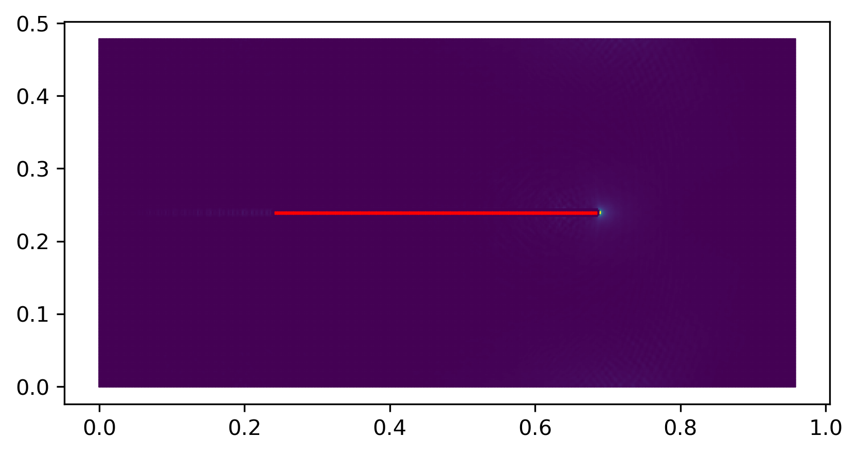
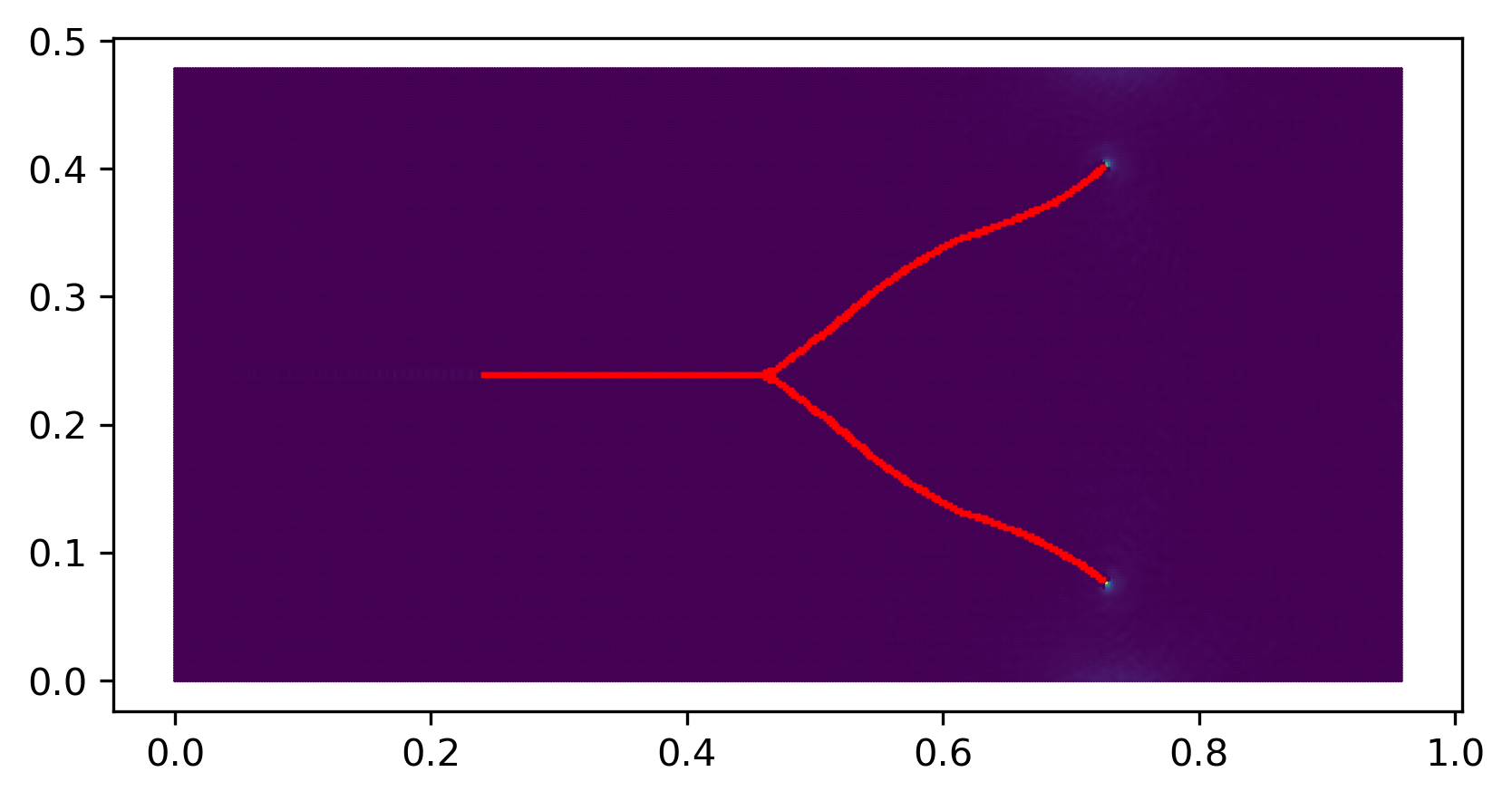
Figure 6: Straight crack and a bifurcated crack due to external body force densities 0.2 GPa and 0.3 GPa, respectively. The red color represents the computed crack.

Our simulations are carried out for the loading considered in Section 7. For this case, it is shown that cracks travel along a straight line and for larger loading they bifurcate [28], [6]. The simulations of Section 9.1 reveal that the crack travels along a straight line behind a localized strain concentration as considered theoretically in Section 7. For larger loading the crack is seen to bifurcate. Observational evidence and rational for bifurcation are experimentally and theoretically identified in [28]. We examine strain energy density inside the intact material before and after branching. Before and after the crack branches the crack path is seen to follow the maximum strain energy of intact material taken over the domain. The simulations explicitly show it to be in front of the crack tip. This is in accord with the experiments of [29] showing that crack path is determined by maximal energy density dissipation.

9.1 Simulation setup and results

We consider a rectangular domain of length $L_{0}=960$ mm and width $L_{0}/2=$ 480 mm with a horizontal pre-notch of length $\frac{L_{0}}{4}=240$ mm starting at the left edge of the domain (see Fig. 5). An external body force density of $\bar{\boldsymbol{b}}=0.2$ GPa and $0.3$ GPa are applied to the top and and bottom $\bar{\epsilon}$-strip of the domain. The initial displacement and velocity are set to zero. The domain is discretized uniformly with mesh size $\bar{h}=2$ mm. The peridynamic horizon size is taken to be $\bar{\epsilon}=6$ mm. The material properties are listed in Table 1.

Young’s modulus ($E$) 72 GPa
Critical energy release rate ($G_{c}$) 135 J/m2
Density ($\rho$) 2440 kg/m3
Poisson ratio ($\nu$) 0.33
Table 1: Material parameters used in simulations

The nonlinear potential function considered here is given by

$\displaystyle{g}(r)={C}(1-e^{-{\beta}{r}^{2}})$

where ${C},{\beta}>0$. The influence function is taken to be

$\displaystyle J(r)=1-r.$

Given the shear modulus $\mu$ and the critical energy release rate $\mathcal{G}_{c}$, in dimension $d=2$, (6.3), (5.12) give

$\displaystyle{C}=3\pi\mathcal{G}_{c},\ {\beta}=\frac{16\mu}{\pi{\mathcal{G}_{c}}},\ r^{c}=\frac{1}{\sqrt{2{\beta}}}.$ (9.3)

Note that, the model parameters ${\beta}$ and ${C}$ are independent of the peridynamic horizon size ${\epsilon}$. This model is simple to use and theoretically breaks bonds only when the displacement ceases to be Hölder continuous (with Hölder exponent 1/2). Since $g^{\prime}(r)$ decays to zero rapidly after $r=r^{c}$, we choose to break bonds stretched beyond $3r^{c}$. For this case bonds sustain $5\%$ force relative to the maximum force.

The numerical simulation is performed using the velocity-Verlet scheme with time step size Δt=5×10⁷Δ𝑡5superscript107\Delta t=5\times 10^{-7} s. At the start of the simulation, all peridynamic bonds intersecting with the pre-notch are removed.
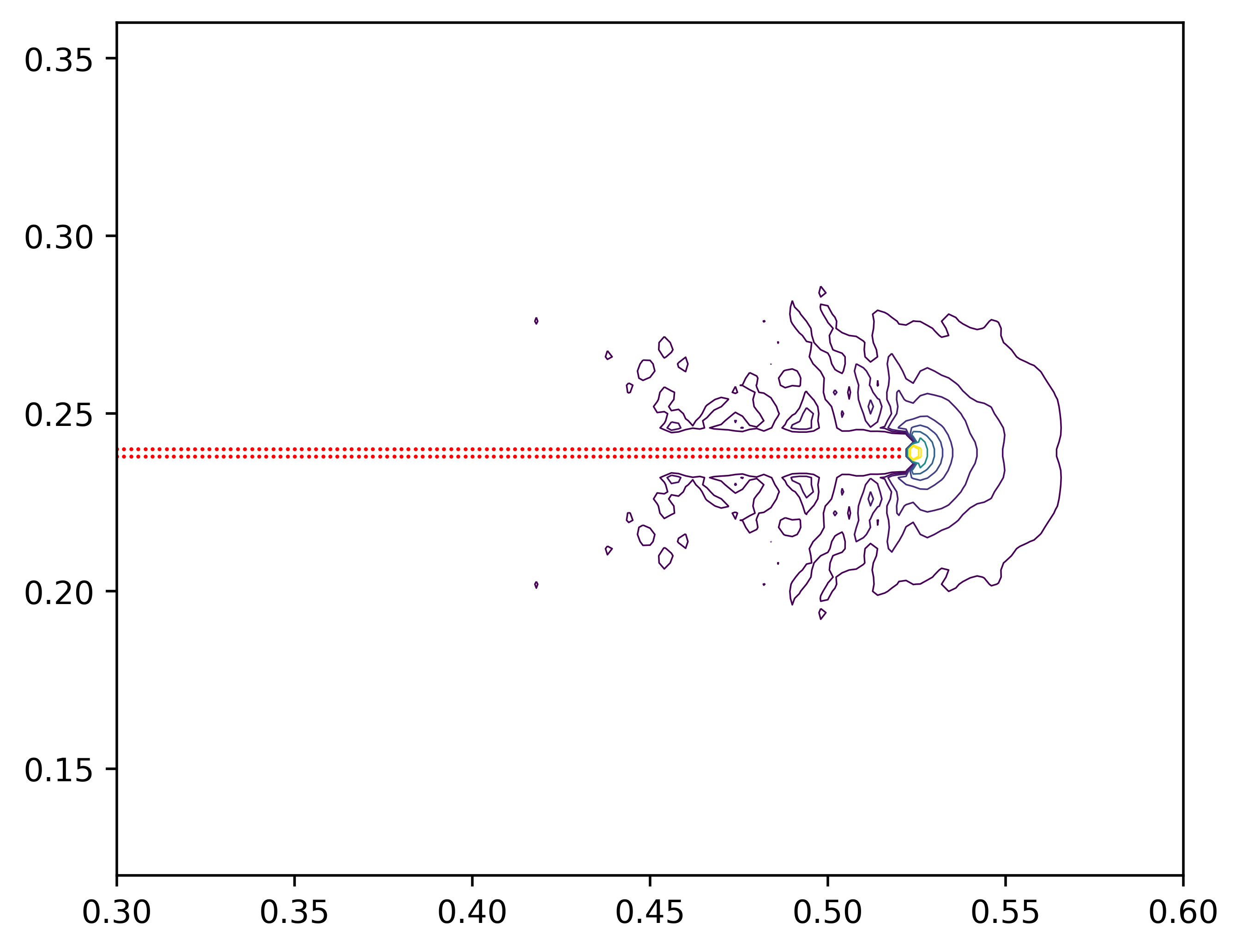
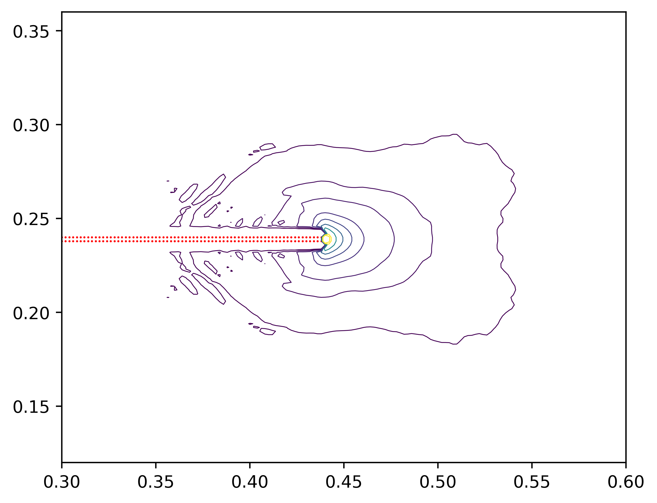
 For a body force density of 0.20.20.2 GPa, the crack propagates in a straight line. For a larger body force density 0.30.30.3 GPa, the crack initially grows in a straight line until it branches at time t=535𝑡535t=535 μ𝜇\mus. The branching behavior is consistent with dynamic simulations seen in [14]. The snapshots of the simulations at t = 900 μ𝜇\mus are shown in Figure 6, where the red color represents the computed crack. 
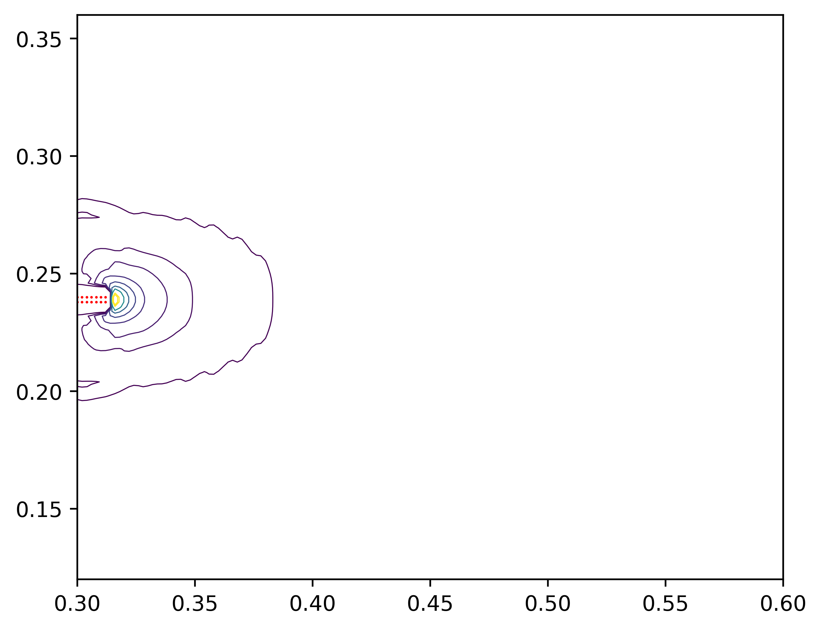
The maximum strain energy density in the domain is observed to be in front of the crack tip, leading the direction of crack growth [29]. 
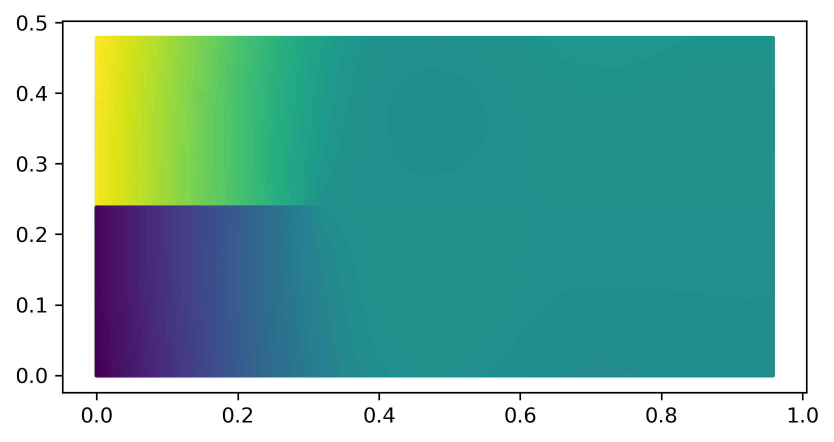
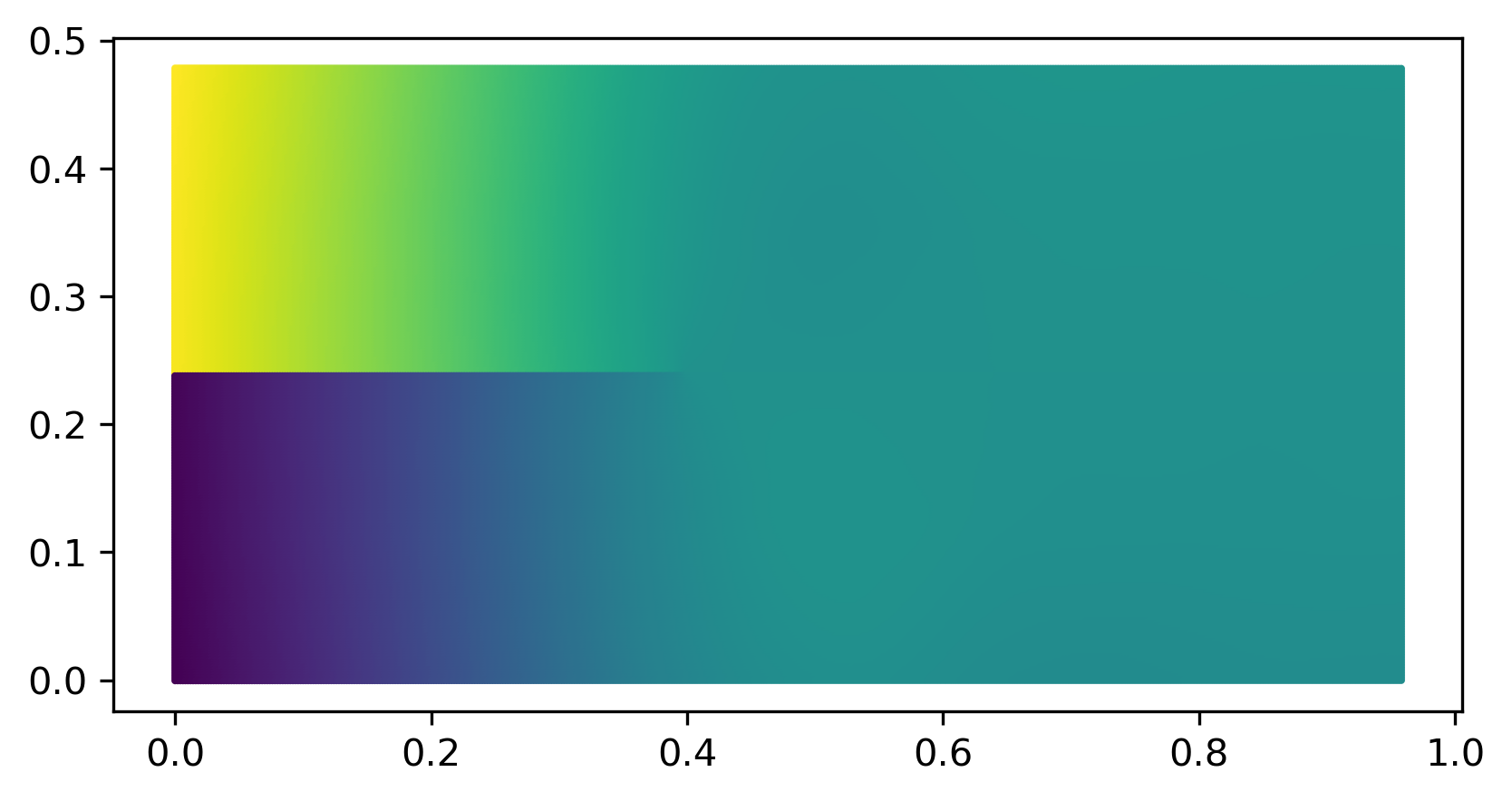
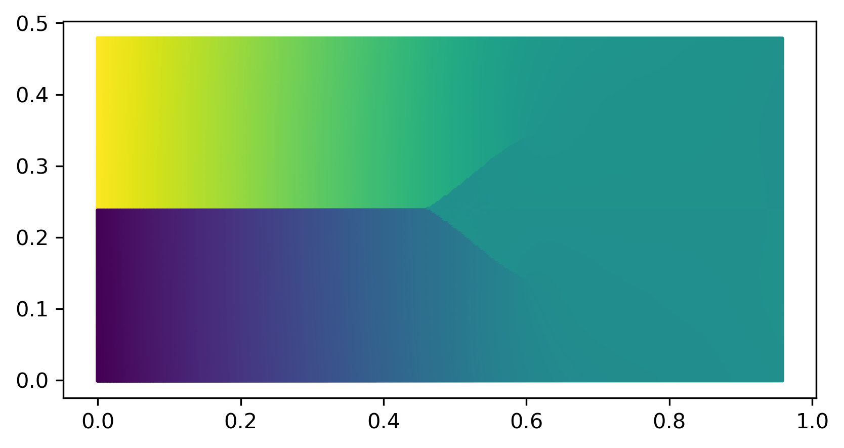
The vertical displacement of all points in the domain at t = 450 and 700 μ𝜇\mus are shown in Figure 7. Here, the jump set of the displacement field denotes the crack path.
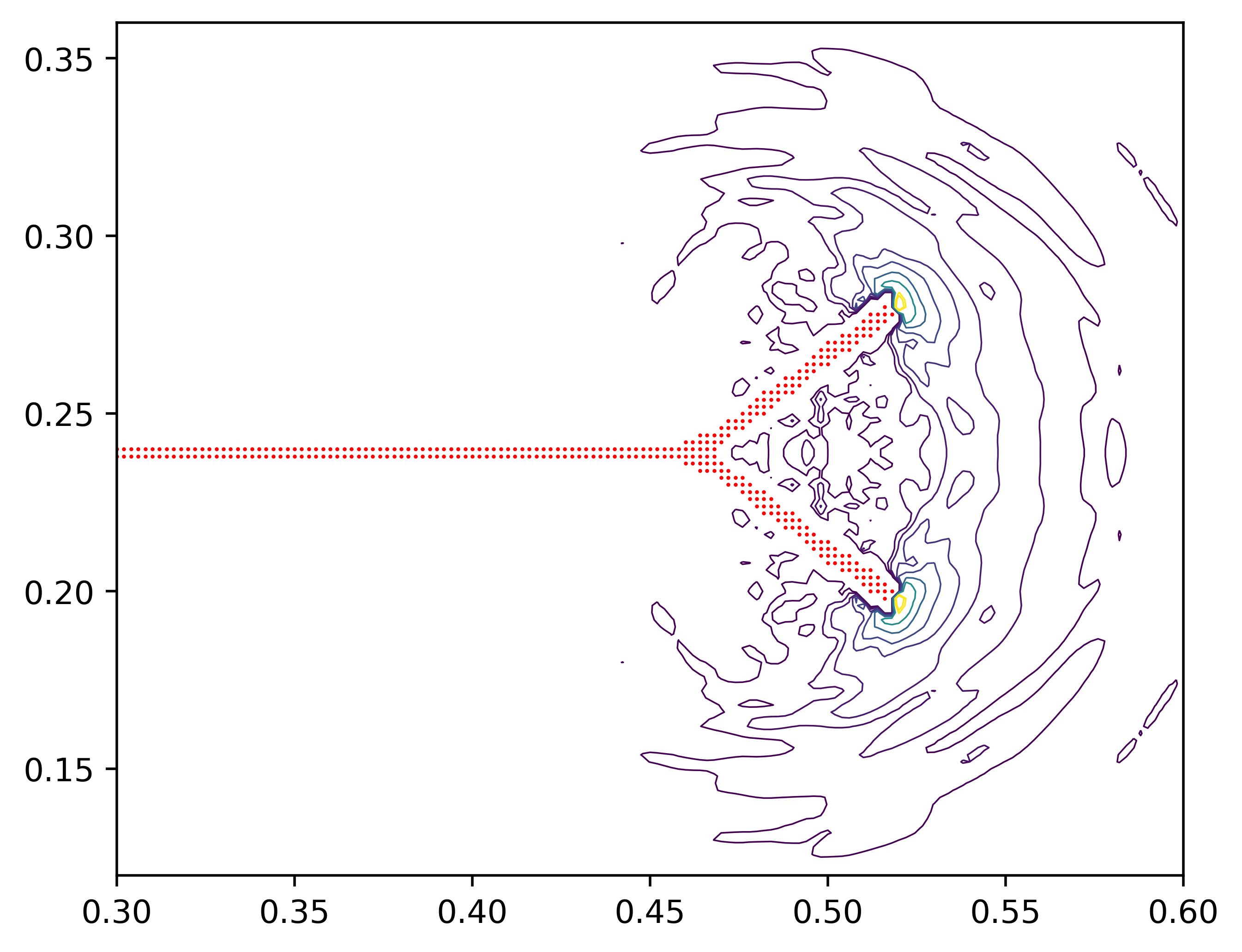
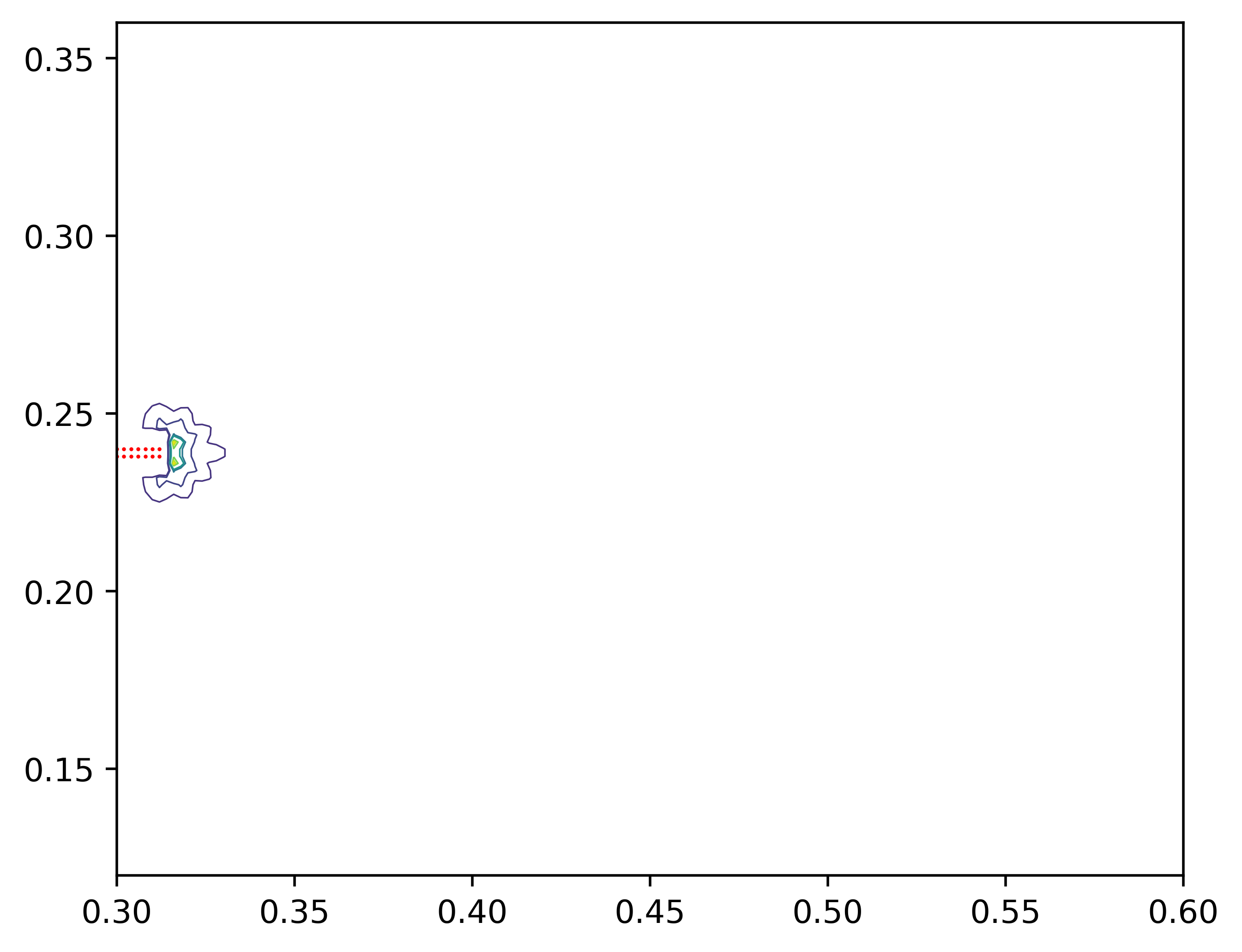
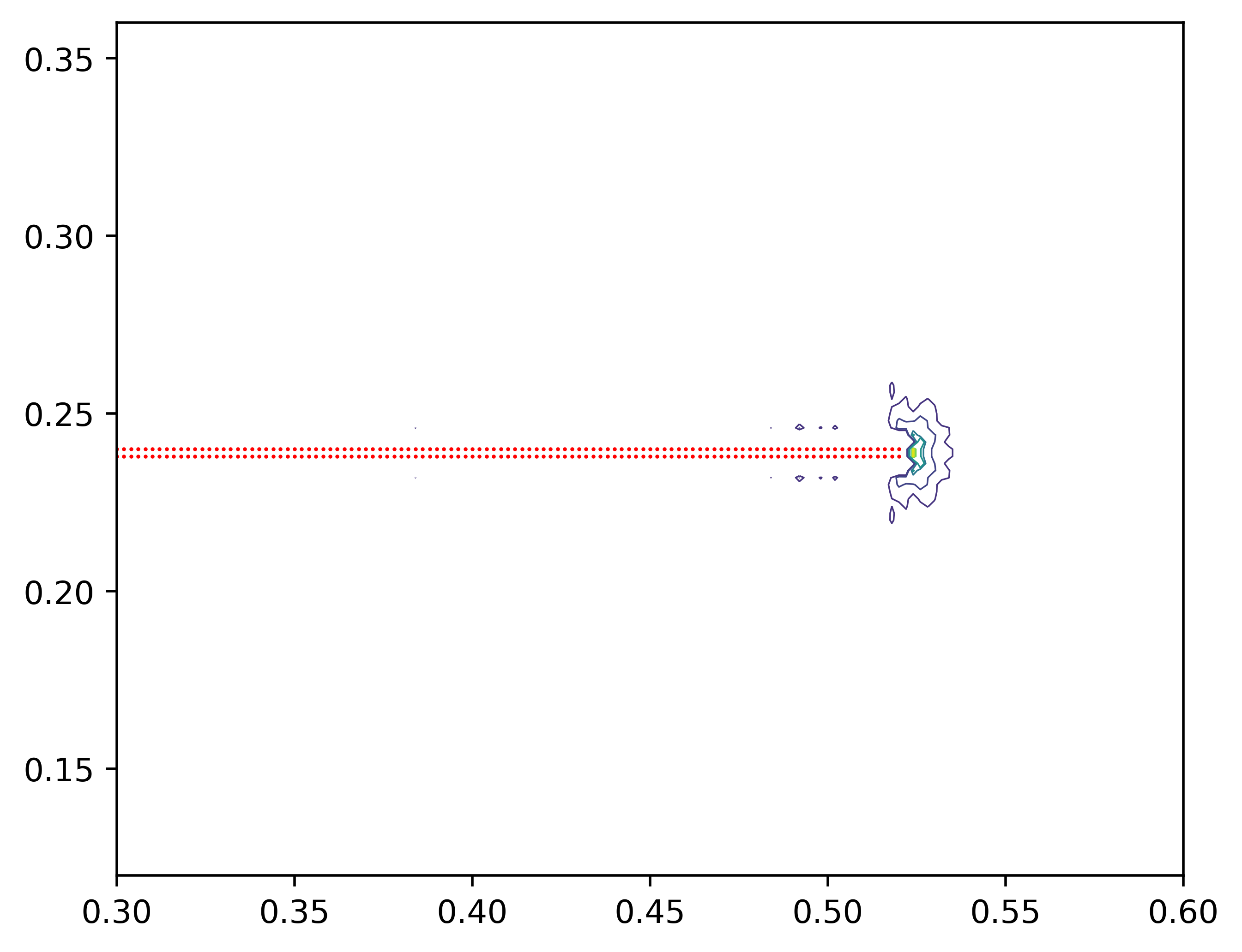
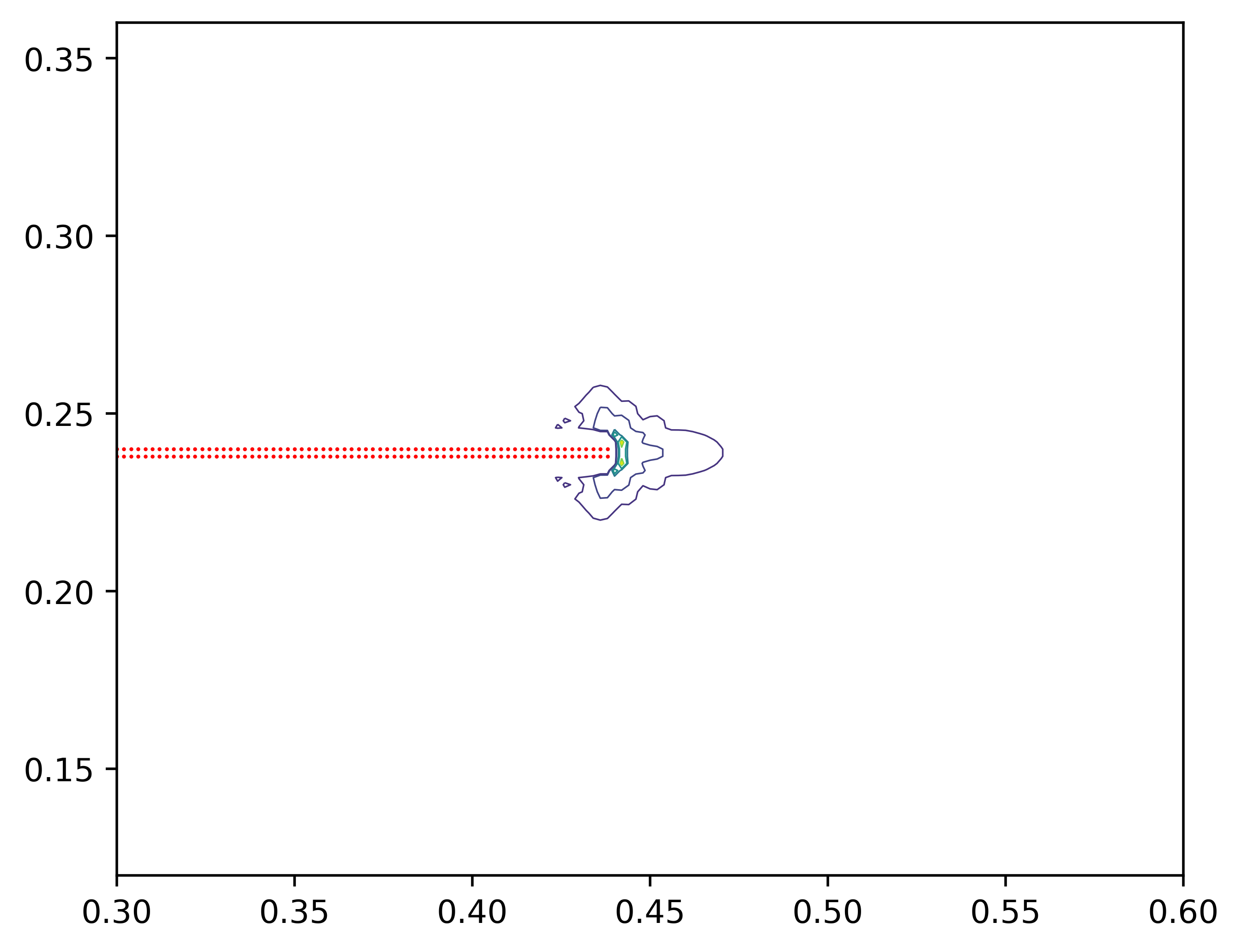
 In Figure 8, we show 
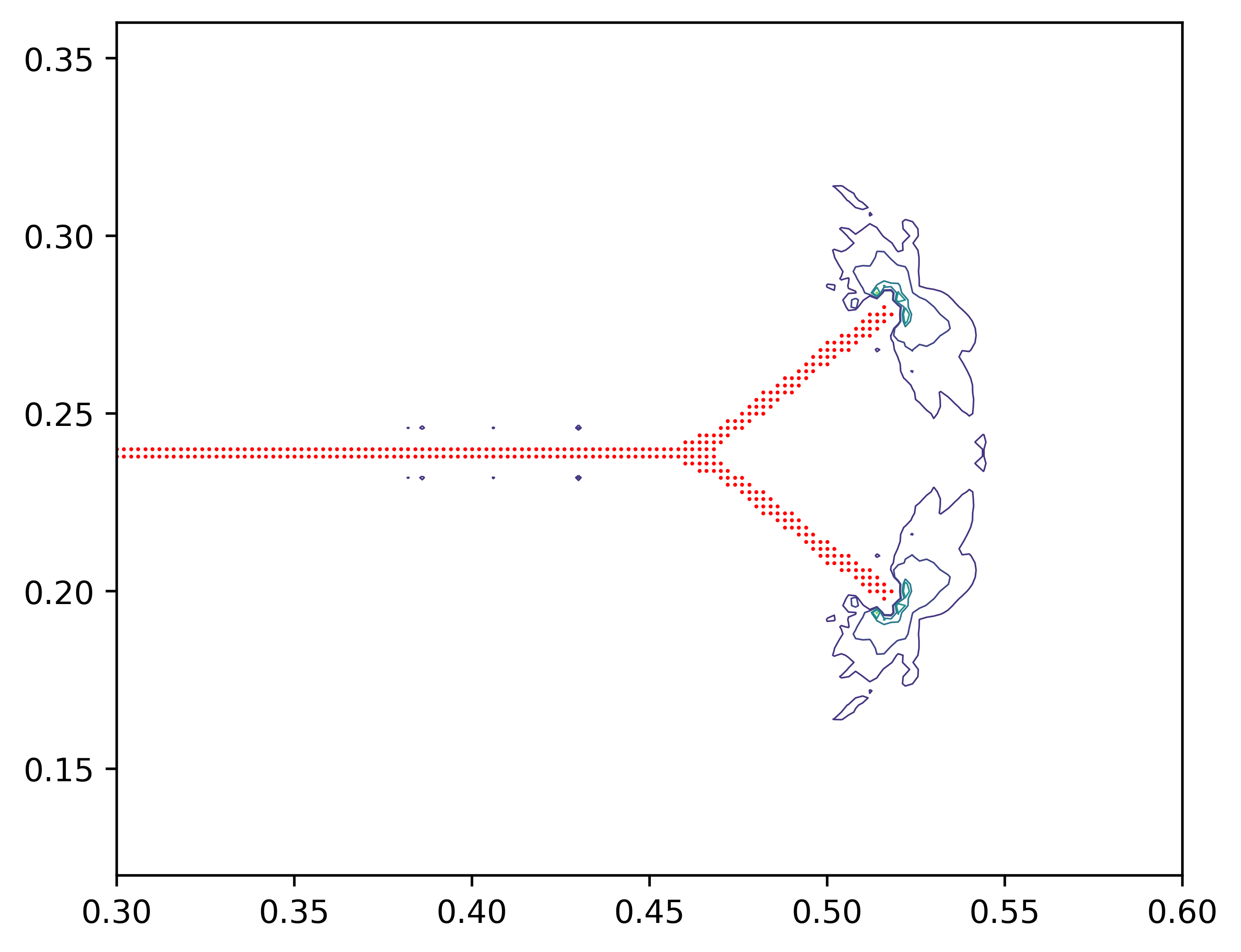
the contour lines of the strain energy density field directly in front of the crack tip. For the straight crack, this is shown at two different crack lengths. For the bifurcating crack, we show the contour lines before and after the crack is bifurcated. The contour lines associated with the stress concentration Z(𝐱,𝐮)𝑍𝐱𝐮Z(\mathbf{x},\mathbf{u}) are shown in Figure 9.

10 Conclusion

The free discontinuity problem for fracture mechanics is rigorously pursued and a model is proposed that demonstrably preserves energy balance and used to discover new advantages to the nonlocal approach. A complete articulation of a theory for a material undergoing irreversible damage guaranteeing energy balance is given. The explicit formula for the energy necessary for material failure and the size of a $d-1$ dimensional “fracture” set is discovered and follows directly from the initial value problem. These results follow immediately when the evolution equation is multiplied by the velocity and an integration by parts is performed.

Material failure is associated with a maximum energy dissipation condition of each bond and the energy of failure agrees with classic Griffith fracture energies for flat internal boundaries. Simulations show that cracks follow the location of maximum energy dissipation inside the intact material. The cracks appear as traction free internal boundaries and both simulation and theory show that they form the wake behind a moving strain concentration consistent with Linear Elastic Fracture Mechanics.

Acknowledgments

This material is based upon work supported by the U. S. Army Research Laboratory and the U. S. Army Research Office under Contract/Grant Number W911NF-19-1-0245. Portions of this research were conducted with high performance computing resources provided by Louisiana State University (http://www.hpc.lsu.edu).

Refer to caption
Refer to caption
Refer to caption
Refer to caption
Figure 7: Displacement $u_{y}$ is shown for two cracks at t = 450, 700 $\mu$s. The jump set in the displacement field reveals the evolving crack.
Refer to caption
Refer to caption
Refer to caption
Refer to caption
Figure 8: The contour lines of strain energy density $W^{\epsilon}(\mathbf{x},\mathbf{u})$ in front of the crack tip are shown. For the straight crack, snapshots at time t = 450, 700 $\mu$s are shown. For the bifurcating crack, we show the snapshots at time $t=500,600\mu$s. The red color represents the crack path. Level curves of strain energy density over the entire domain show maximum strain energy is achieved directly in front of the crack tip.
Refer to caption
Refer to caption
Refer to caption
Refer to caption
Figure 9: The contour lines of strain concentration $Z^{\epsilon}(\mathbf{x},\mathbf{u})$ in the intact material are shown, i.e. for points with $0\leq Z\leq 1$. For the straight crack, snapshots at time t = 450, 700 $\mu$s are shown. For the bifurcating crack, we show the snapshots at time $t=500,600\mu$s. The red color represents the crack path.

References

  • [1] Y. Bazilevs, M. Behzadinasab, and J. Foster. Simulating concrete failure using the microplane (M7) constitutive model in correspondence-based peridynamics: Validation for classical fracture tests and extension to discrete fracture. J. Mech. Phys. Solids, 166, 2022.
  • [2] D. Bhattacharya, R. Lipton, and P. Diehl. Quasistatic fracture evolution using a nonlocal cohesive model. International Journal of Fracture, doi.org/10.1007/s10704-023-00711-0, 2023.
  • [3] D. Bhattacharya and R. P. Lipton. Quasistatic evolution with unstable forces. Multiscale Modeling & Simulation, 21(2):598–623, 2023.
  • [4] K. Bhattacharya and K. Dayal. Kinetics of phase transformationa in the peridynamic formulation of continuum mechanics. Journal of the Mechanics and Physics of Solids, 54:1811–1842, 2006.
  • [5] F. Bobaru, J. T. Foster, P. H. Geubelle, and S. A. Silling. Handbook of peridynamic modeling. CRC press, 2016.
  • [6] F. Bobaru and G. Zhang. Why do cracks branch? a peridynamic investigation of dynamic brittle fracture. International Journal of Fracture, 196:59–98, 2015.
  • [7] G. Dal Maso and R. Toader. On the Cauchy problem for the wave equation on time dependent domains. J. Differ. Equ., 266:3209–3246, 2019.
  • [8] P. Diehl, R. Lipton, T. Wick, and M. Tyagi. A comparative review of peridynamics and phase-field models for engineering fracture mechanics. Computational Mechanics, pages 1–35, 2022.
  • [9] Q. Du, M. Gunzburger, R. Lehoucq, and K. Zhou. Analysis of the volume-constrained peridynamic navier equation of linear elasticity. Journal of Elasticity, 113:193–217, 2013.
  • [10] Q. Du, Y. Tao, and X. Tian. A peridynamic model if fracture mechanics with bond-breaking. J. Elasticity, 2015.
  • [11] E. Emmrich and D. Phust. A short note on modeling damage in peridynamics. J. Elasticity, 2015.
  • [12] H. Federer. Geometric Measure Theory. Springer, 1969.
  • [13] J. Foster, S. Silling, and W. Chen. An energy based failure criterion for use with peridynamic states. International Journal of Fracture, 9:679–688, 2011.
  • [14] Y. D. Ha and F. Bobaru. Studies of dynamic crack propagation and crack branching with peridynamics. International Journal of Fracture, 162:229–244, 2010.
  • [15] Y. Hu, H. Chen, B. W. Spencer, and E. Madenci. Thermomechanical peridynamic analysis with irregular non-uniform domain discretization. Engineering Fracture Mechanics, 197:92–113, 2018.
  • [16] Y. Hu and E. Madenci. Bond-based peridynamic modeling of composite laminates with arbitrary fiber orientation and stacking sequence. Composite structures, 153:139–175, 2016.
  • [17] M. Isiet, I. Mišković, and S. Mišković. Review of peridynamic modelling of material failure and damage due to impact. International Journal of Impact Engineering, 147:103740, 2021.
  • [18] S. Jafarzadeh, F. Mousavi, A. Larios, and F. Bobaru. A general and fast convolution-based method for peridynamics: Applications to elasticity and brittle fracture. Computer Methods in Applied Mechanics and Engineering, 392:114666, 2022.
  • [19] A. Javili, R. Morasata, E. Oterkus, and S. Oterkus. Peridynamics review. Mathematics and Mechanics of Solids, 24(11):3714–3739, 2019.
  • [20] P. K. Jha and R. Lipton. Kinetic relations and local energy balance for LEFM from a nonlocal peridynamic model. International Journal of Fracture, 226(1):81–95, 2020.
  • [21] R. Lipton. Dynamic brittle fracture as a small horizon limit of peridynamics. Journal of Elasticity, 117(1):21–50, 2014.
  • [22] R. Lipton. Cohesive dynamics and brittle fracture. Journal of Elasticity, 124(2):143–191, 2016.
  • [23] R. Lipton, E. Said, and P. Jha. Free damage propagation with memory. Journal of Elasticity, 133(2):129–153, 2018.
  • [24] R. P. Lipton and P. K. Jha. Nonlocal elastodynamics and fracture. Nonlinear Differential Equations and Applications, 2021.
  • [25] R. P. Lipton, R. B. Lehoucq, and P. K. Jha. Complex fracture nucleation and evolution with nonlocal elastodynamics. Journal of Peridynamics and Nonlocal Modeling, 1(2):122–130, 2019.
  • [26] E. Madenchi and Oterkus. Peridynamic theory. In IPerydynamic theory and its applications, pages 19–43. Springer, New York, 2013.
  • [27] F. Morgan. Geometric Measure Theory, A Beginners Guide. Springer-Verlag, Berlin, 19955.
  • [28] K. Ravi-Chandar and W. G. Knauss. An experimental investi- gation into dynamic fracture: III. on steady-state crack propagation and crack branching. Int J Fract, 26:141–154, 1984.
  • [29] L. Rozen-Levy, J. M. Kolinski, G. Cohen, and J. Fineberg. How fast cracks in brittle solids choose their path. Physical Review Letters, 125(17):175501, 2020.
  • [30] P. Seleson and D. Littlewood. Convergence studies in meshfree peridynamic simulations. Computers & Mathematics with Applications, 71:2432–2448, 2018.
  • [31] S. Silling and E. Ascari. A mesh free method based on the peridynamic model of solid mechanics. Comput. Struct, 83:1526–1536, 2005.
  • [32] S. A. Silling. Reformulation of elasticity theory for discontinuities and long-range forces. Journal of the Mechanics and Physics of Solids, 48(1):175–209, 2000.
  • [33] S. A. Silling, M. Epton, O. Weckner, J. Xu, and E. Askari. Peridynamic states and constitutive modeling. Journal of Elasticity, 88(2):151–184, 2007.
  • [34] Z. Xu, G. Zhang, Z. Chen, and F. Bobaru. Elastic vortices and thermally-driven cracks in brittle materials with peridynamics. International Journal of Fracture, 209:203–222, 2018.
  • [35] M. Zaccaritto, F. Luongo, G. Sargeo, and U. Galvanetto. Examples of applications of the peridynamic theory to the solution of static equilibrium problems. The Aeronautical Journal, 119:677–700, 2015.