Scaling dimension of $4\pi$-flux monopole operator in four-flavor three-dimensional QED using lattice simulation

Abstract

We numerically address the issue of which monopole operators are relevant under renormalization group flow in three-dimensional parity-invariant noncompact QED with $4$ flavors of massless two-component Dirac fermion. Using lattice simulation and finite-size scaling analysis of the free energy to introduce monopole-antimonopole pairs in $N=4$ and $N=12$ flavor noncompact QED₃, we estimate the infrared scaling dimensions of monopole operators that introduce $2\pi$ and $4\pi$ fluxes around them. We first show that the estimates for the monopole scaling dimensions are consistent with the large-$N$ expectations for $N=12$ QED₃. Applying the same procedure in $N=4$ QED₃, we estimate the scaling dimension of $4\pi$ flux monopole operator to be $3.7(3)$, which allows the possibility of the operator being irrelevant. This finding offers support to the scenario in which higher-flux monopoles are irrelevant deformations to the Dirac spin liquid phase that could be realized on certain non-bipartite lattices by forbidding $2\pi$-flux monopoles.

I Introduction

The characterization of the quantum numbers of monopoles in the continuum and on various lattices, and their impact on the infrared behavior of three-dimensional quantum electrodynamics coupled to even number of flavors ($N$) of massless two-component Dirac fermions have been topics of interest in recent times. The presence and absence of monopoles are expected to change the long-distance behavior of QED₃ radically. QED₃ without monopole excitation – noncompact QED₃ – has been intensely studied using various methods, for example, using lattice regularization Hands and Kogut (1990); Hands et al. (2002, 2004); Raviv et al. (2014), conformal bootstrap Chester and Pufu (2016); Chester et al. (2018); He et al. (2022); Li (2022); Albayrak et al. (2022); Rychkov and Su (2023), Dyson-Schwinger approaches Pisarski (1984); Appelquist et al. (1985, 1986a, 1986b, 1988); Gusynin and Reenders (2003); Gusynin and Pyatkovskiy (2016); Kotikov et al. (2016). Ab initio numerical studies using the lattice regularization with exactly massless fermions and finite-size scaling have shown that parity-invariant non-compact QED₃ exhibits scale-invariant behavior independent of the number of flavors; some salient observations toward this conclusion stems from finite-size scaling of low-lying Dirac eigenvalues Karthik and Narayanan (2016a, b) and closer resemblance of their eigenvalue distributions to those from a simple conformal model Karthik and Narayanan (2020), and presence of power-law correlators Karthik and Narayanan (2016b, 2017). Despite the term noncompact, it should be emphasized that the fermions see a compact version of the gauge field in the lattice regularization. On the other hand, QED₃ with any number of monopoles – compact QED₃ – without massless fermion content is well known to be confined Polyakov (1975, 1977).

Even though monopoles do not arise dynamically in the noncompact theory after the ultraviolet regulator is removed, one could subject the noncompact theory to monopole-like singular boundary conditions at various space-time points; for a flux $Q$ monopole, the total flux  on surfaces enclosing the point is $2\pi Q$ for integers $Q$. For fermions coupled to the U(1) gauge fields, the extended Dirac string singularity is invisible, and the insertion of the monopole behaves like the insertion of a composite operator at the point. Hence, one defines the monopole operator ${\cal M}_{Q}(x)$ through its action of introducing $2\pi Q$ flux around the point $x$ Borokhov et al. (2002). At critical points of a U(1) lattice theory, one can find the scaling dimension of such monopole operators via the two-point functions,

$$\left\langle{\cal M}^{\dagger}_{Q}(x){\cal M}_{Q}(0)\right\rangle\propto|x|^{-2\Delta_{Q}}.$$ (1)

The exponent $\Delta_{Q}$ is the scaling dimension of ${\cal M}_{Q}$. Since criticality is approached only in the long-distance or the infrared limit of QED₃, the above power-law scaling will be seen when the monopole and antimonopole are separated by large distances. If the infrared dimension $\Delta_{Q}>3$, then flux-$Q$ monopoles are irrelevant to the infrared end of the renormalization group flow.

The nature of compact QED₃ coupled to exactly massless fermions is yet unresolved. A lattice study of compact QED₃ is complicated by the inherent singular nature of monopoles Karthik and Narayanan (2019a) and the presence of near-zero Dirac operator eigenmodes away from the massless limit even as one decreases the lattice spacing. It is conceivable that a naive continuum limit of compact QED₃ with massless fermions in a traditional sense (that is, an approach to continuum limit at the Gaussian fixed point as the lattice coupling is taken to zero keeping physical scales fixed) is not well-defined. Refs Hands et al. (2006); Armour et al. (2011) studied this theory in the presence of a four-fermi interaction. Another option might be to UV complete compact QED₃ using a SU(2) theory in the presence of a Higgs field Polyakov (1977). A quantum Monte-Carlo study Xu et al. (2019) instead focused on a U(1) lattice gauge theory coupled to many flavors of staggered fermions and its strong-to-weak coupling phase diagram. This fundamental difficulty associated with a direct numerical study of the UV-IR renormalization group flows in compact QED₃ in the continuum limit provides a strong motivation to study the scaling dimension of monopole operators in the noncompact version of the theory. In compact QED₃, monopoles of all $2\pi Q$ fluxes dynamically appear. As $\Delta_{Q}$ is typically a monotonically increasing function of $Q$, if $\Delta_{1}$ of the $Q=1$ monopole is greater than 3 in an $N$ flavor noncompact QED₃, then one expects a similar conformal behavior in the $N$-flavor compact QED₃ and noncompact QED₃. In this way, the $Q=1$ monopole is expected to be relevant only for $N<12$ based on large-$N$ and $4-\epsilon$ approximations Pufu (2014); Chester et al. (2016), and further confirmed by lattice simulations in previous as well as in the present work. By the above argument, the compact QED₃ is expected to have a critical number of flavor $N\approx 12$.

Given the dominant role of the monopole creating the smallest $2\pi$ flux, a study of higher flux-creating monopoles might not seem significant. However, the specific motivation for studying monopoles that create $4\pi$ flux in this work is the following. Recently, there has been interest in a realization of compact QED₃ where the dominant $Q=1$ monopole is disallowed due to ultraviolet symmetries specific to certain lattices Song et al. (2020). Such a version of $N=4$ compact QED₃ that is devoid of $Q=1$ monopole is expected to be an effective field theory description of the antiferromagnetic Heisenberg spin model on Kagomé and triangular lattices that could host a Dirac spin liquid (DSL) phase Song et al. (2020, 2019); Zhu et al. (2018). Whereas the stability of DSL on a triangular lattice is also decided by the requirement of irrelevance of an allowed four-fermi term that is close to being marginal, the $Q=2$ monopole was argued Song et al. (2019) to be the critical object determining the stability of DSL on Kagomé lattices. At the present accuracy of the large-$N$ expansion of QED₃, the scaling dimension of the $Q=2$ monopole operator is approximately 2.5. Since this value is quite close to the marginal value of 3, it is possible that the higher-order perturbative corrections and genuine nonperturbative corrections to the large-$N$ value at the relatively small $N=4$ could shift the actual value of the monopole scaling dimension to be greater than 3. Therefore, the possibility of the long-distance correlation in the DSL phase on the two non-bipartite lattices, especially on the Kagomé lattice, is then tied to the infrared conformality of the $N=4$ compact QED₃ in the absence of $Q=1$ monopoles; in other terms, to the infrared irrelevance of the next-allowed $Q=2$ monopole operators in $N=4$ noncompact QED₃. The nonperturbative determination of the scaling dimension of the $Q=2$ monopoles in $N=4$ noncompact QED₃ using direct lattice simulation is therefore the main aim of this paper.

II Method

II.1 Lattice regulated noncompact QED₃ and monopole insertions therein

The parity-invariant noncompact theory consists of Abelian gauge fields $A_{\mu}(x)$ coupled to an even number of flavors, $N$, of massless two-component Dirac fermions. The gauge coupling $g^{2}$ in the theory has a mass dimension of 1, which makes the theory super-renormalizable and we can use appropriate factors of $g^{2}$ to make all masses and lengths dimensionless. We study the lattice regulated version of the theory on a periodic box of dimensionless physical volume $\ell^{3}$ that is discretized using a lattice of size $L^{3}$. The continuum limit of the finite volume theory can be obtained by extrapolating to $L\to\infty$ limit in different fixed physical extents $\ell$.

We take a brief detour to formally define noncompact gauge theory that is explicitly a U(1) gauge theory, and define monopole insertions within this U(1) lattice gauge theory. The Villain formulation Villain (1975) of the noncompact QED₃ can be defined via the path integral,

$$Z=\left(\prod_{x,\mu}\int_{-\infty}^{\infty}d\theta_{\mu}(x)\right)\det{}^{N/2}\left[\not{C}\not{C}^{\dagger}\right]{\cal W}_{g}(\theta),$$ (2)

where $\not{C}$ is a two-component lattice Dirac operator that is coupled to the lattice gauge fields $\theta_{\mu}(x)=A_{\mu}(x)\ell/L$ via the compact variable $U_{\mu}(x)=e^{i\theta_{\mu}(x)}$. The theory is regulated in a parity-invariant manner by coupling $N/2$ flavors to $\not{C}$, and the other $N/2$ to $\not{C}^{\dagger}$. The contribution from the gauge sector is ${\cal W}_{g}(\theta)$ given by,

$${\cal W}_{g}(\theta)=\sum_{\{N_{\mu\nu}\}}\exp\left[-\frac{L}{\ell}\sum_{x}\sum_{\mu>\nu}\left(F_{\mu\nu}(x)-2\pi N_{\mu\nu}(x)\right)^{2}\right]\quad\text{where}\quad F_{\mu\nu}(x)=\Delta_{\mu}\theta_{\nu}(x)-\Delta_{\nu}\theta_{\mu}(x).$$ (3)

with the sum over configurations of integer values $N_{\mu\nu}(x)$ associated with the $(\mu,\nu)$-plaquette at site $x$. Since both ${\cal W}_{g}(\theta)$ and the Dirac operator $\not{C}$ are invariant under shifts $\theta_{\mu}(x)\to\theta_{\mu}(x)+2\pi n_{\mu}(x)$ for integers $n_{\mu}(x)$, the path-integral Eq. (2) is that of U(1) gauge theory coupled to fermions. The magnetic charge $Q(x)$ of the monopole at a site $x$ is defined DeGrand and Toussaint (1980) via the divergence of an integer-valued current dual to $N_{\mu\nu}(x)$; that is,

$$Q(x)\equiv\frac{1}{2}\sum_{\mu,\nu,\rho}\epsilon_{\mu\nu\rho}\Delta_{\mu}N_{\nu\rho}(x).$$ (4)

For the sake of brevity, we simply define a monopole at a point $x$ with a value of net flux as $2\pi Q$ as a flux-$Q$ monopole. Depending on the constraints on the allowed values of $Q(x)$ in the path-integral, which thereby corresponds to constraints on the allowed configurations $\{N_{\mu\nu}\}$ in Eq. (3), one can define different versions of QED₃. The noncompact QED₃ is the U(1) gauge theory with the constraint, $Q(x)=0$, at all $x$ in the continuum limit of the lattice-regulated theory. In this case, by making use of the invariance of theory under $\theta_{\mu}\to\theta_{\mu}+2\pi n_{\mu}$ shifts, one can write down the path-integral in the usual form without any sum over $N_{\mu\nu}$ as

$$Z_{0}=\left(\prod_{x,\mu}\int_{-\infty}^{\infty}d\theta_{\mu}(x)\right)\det{}^{N/2}\left[\not{C}\not{C}^{\dagger}\right]e^{-\frac{L}{\ell}\sum_{x}\sum_{\mu>\nu}F_{\mu\nu}(x)^{2}}.$$ (5)

We can define the path-integral $Z_{Q}$ with a flux-$Q$ monopole inserted at a point $x^{\prime}$ and an antimonopole at a point $x^{\prime}+r$ by subjecting to the constraint $N_{\mu\nu}(x)=N^{Q\bar{Q}}_{\mu\nu}(x;r)$ with

$$\frac{1}{2}\sum_{\mu,\nu,\rho}\epsilon_{\mu\nu\rho}\Delta_{\mu}N^{Q\bar{Q}}_{\nu\rho}(x;r)=Q\delta_{x,x^{\prime}}-Q\delta_{x,x^{\prime}+r}.$$ (6)

The two-point function of a monopole at $x^{\prime}$ and $x^{\prime}+r$ is simply the ratio, $Z_{Q}/Z_{0}$.

The universal aspects like the anomalous dimensions at the infrared fixed point should not be sensitive to the exact details of the lattice operator so long as the operator quantum numbers are captured correctly. Therefore, we can choose the type of background flux to better capture the effect of monopole operators. Instead of introducing integer-valued flux $N^{Q\bar{Q}}_{\mu\nu}$ in the path-integral, we follow the approach of Refs Murthy and Sachdev (1990); Pufu and Sachdev (2013) to introduce a classical background gauge field ${\cal A}^{Q\bar{Q}}_{\mu}(x;r)$ that minimizes the pure gauge action

$$S_{g}=\left[B_{\mu\nu}^{Q\bar{Q}}(x;r)-2\pi N^{Q\bar{Q}}_{\mu\nu}(x;r)\right]^{2};\qquad B_{\mu\nu}^{Q\bar{Q}}(x;r)=\Delta_{\mu}{\cal A}^{Q\bar{Q}}_{\nu}(x;r)-\Delta_{\nu}{\cal A}^{Q\bar{Q}}_{\mu}(x;r),$$ (7)

on a periodic box. We then define the path-integral in the presence of monopole insertions via,

$$Z_{Q}=\left(\prod_{x,\mu}\int_{-\infty}^{\infty}d\theta_{\mu}(x)\right)\det{}^{N/2}\left[\not{C}\not{C}^{\dagger}\right]e^{-\frac{L}{\ell}\sum_{x}\sum_{\mu>\nu}\left(F_{\mu\nu}(x)-QB^{1\bar{1}}_{\mu\nu}(x;r)\right)^{2}},$$ (8)

using the fact that $B_{\mu\nu}^{Q\bar{Q}}=QB_{\mu\nu}^{1\bar{1}}$. The above procedure has the advantage that the effect of monopole can be completely removed from the path-integral in the pure-gauge theory ($N=0$) by redefining the dynamical gauge field $\theta_{\mu}(x)\to\theta_{\mu}(x)-{\cal A}^{Q\bar{Q}}_{\mu}(x;r)$. Therefore any non-zero effect of the monopole at finite non-zero $N$ can arise only due to the presence of massless fermions. This procedure has been put to test previously in the free fermion theory Karthik (2018), and at the critical point of the 3d XY-model Karthik (2018).

II.2 Monopole correlator and finite-size scaling

The lattice monopole two-point function is given by

$$G_{\mathrm{lat}}(r,\ell,L)=\frac{Z_{Q}}{Z_{0}}.$$ (9)

As with correlators of regular composite operators composed of local fields, we assume that the lattice correlator $G_{\mathrm{lat}}$, which is in units of lattice spacing $a=\ell/L$, can be converted into a correlator in physical units $G_{\mathrm{phys}}$ by a multiplicative factor; namely,

$$G_{\mathrm{phys}}(r,\ell,L)=a^{-2D_{Q}^{(N)}}G_{\mathrm{lat}}(r,\ell,L),$$ (10)

where $D_{Q}^{(N)}$ is the ultraviolet exponent governing the monopole correlator at short distances. We will discuss more on the conversion from the lattice to the physical correlator when presenting the results from our numerical calculation. The physical continuum correlator, $G_{\mathrm{phys}}(r,\ell)$, after extrapolating to $L\to\infty$ will show scale-invariant behavior at large separations $|r|$ and $\ell$ as

$$G_{\mathrm{phys}}(r,\ell)=\frac{1}{|r|^{2\Delta^{(N)}_{Q}}}{\cal G}\left(\frac{|r|}{\ell}\right)\quad\text{as}\quad|r|\to\infty,$$ (11)

for some scaling function ${\cal G}$. The exponent $\Delta^{(N)}_{Q}$ that governs the long-distance correlator is the infrared scaling dimension of the monopole operator that we are seeking. There could be corrections to the above simple scaling from higher-order $1/\ell$ corrections and due to contamination from higher-dimensional flux-$Q$ monopole operators that the background field method could overlap with; we assume such corrections are much smaller compared to the numerical accuracy of our data. By keeping the ratio $|r|/\ell=\rho$ fixed as $\ell$ is increased,

$$G_{\mathrm{phys}}(|r|=\rho\ell,\ell)\propto\frac{1}{\ell^{2\Delta^{(N)}_{Q}}}\quad\text{as}\quad\ell\to\infty.$$ (12)

We will follow this procedure in this work, and keep the monopole-antimonopole separation proportional to box size, thereby reducing the determination of the infrared scaling dimension to a finite-size scaling analysis.

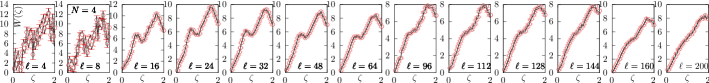
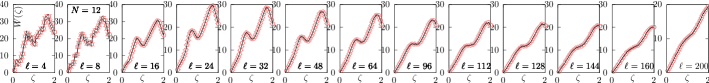
Figure 1: Representative data points and their interpolations for the lattice determined derivative of free energy, $W(\zeta)$, with respect to the auxiliary parameter $\zeta$. The top and bottom panels show results for $W(\zeta)$ at different $\ell$ on $L=24$ lattice in $N=4$ and 12 noncompact QED₃ respectively. The red data points are the actual Monte Carlo determinations. The black bands are the spline interpolations to the data.

II.3 Implementation of the numerical calculation

We studied noncompact theory with $N=4$ and $N=12$ flavors on periodic Euclidean boxes at multiple values of physical extents $\ell=$ 4, 8, 16, 24, 32, 48, 64, 96, 128, 144, 160 and 200. We discretized them on lattices of volume $L^{3}$ with $L=12,16,20,24$ and 28. We used Wilson-Dirac operator $\not{C}_{w}$ that is coupled to 1-step HYP-smeared gauge field. We tuned to the massless point by tuning the bare Wilson fermion mass $m_{w}$ so that the first eigenvalue $\Lambda_{1}^{2}(m_{w})$ of $\not{C}_{w}\not{C}_{w}^{\dagger}$ is minimized as a function of $m_{w}$. More details on the two-component Wilson-Dirac operator and its mass tuning can be in our earlier work in Ref Karthik and Narayanan (2016a).

We chose the displacement vector $r$ between the flux-$Q$ monopole and antimonopole to be along one of the axis; namely, the three-vector $r=(0,0,t)$ for $t=aT$ and integers $T$. We kept $\rho=t/\ell=1/4$, an arbitrary choice in the work to simplify the analysis to a finite-size scaling one as explained before. For this choice of on-axis $r$, a natural choice for $N_{\mu\nu}^{1\bar{1}}$ that satisfies Eq. (6) is $N_{12}^{1\bar{1}}(0,0,x_{3})=1$ for $x_{3}\in[1,T]$, and all other $N_{\mu\nu}^{1\bar{1}}$ are set to 0. Such a choice can be changed arbitrarily by shifts $N_{\mu\nu}^{1\bar{1}}\to N_{\mu\nu}^{1\bar{1}}+\Delta_{\mu}n_{\nu}-\Delta_{\nu}n_{\mu}$ for integers $n_{\mu}(x)$, that move and bend the Dirac string (the column of plaquettes with $2\pi$ flux) keeping the location of monopole and antimonopole fixed; however such variations are unimportant in the U(1) theory, and therefore, the simplest choice above for $N_{12}^{Q\bar{Q}}$ suffices. With this choice of $N_{\mu\nu}^{1\bar{1}}$, we determined the background field ${\cal A}^{1\bar{1}}_{\mu}(x)$, and the field tensor $B^{1\bar{1}}_{\mu\nu}(x)$ in the periodic $L^{3}$ box by analytically minimizing Karthik and Narayanan (2019a) the action Eq. (7). From this, the background field for any value of $Q$ can be obtained as $QB^{1\bar{1}}_{\mu\nu}(x)$.

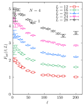
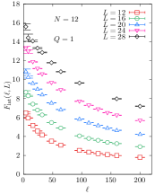
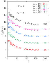
Figure 2: The free energy, $F_{\mathrm{lat}}(\ell,L)$, in lattice units is shown as a function of physical box size, $\ell$. The values of $(Q,N)$ in the panels from left to right correspond to $(1,4),(1,12),(2,4),(2,12)$ respectively. In each panel, the data at $L=12,16,20,24$ and 28 are shown.

The effect of $B^{Q\bar{Q}}_{\mu\nu}$ is exponentially suppressed in Eq. (8), and therefore, it is hard to compute $Z_{Q}$ as an expectation value in $Q=0$ theory. Instead, we follow the approach in Ref Karthik (2018), and computed the logarithm of the above correlator, which is nothing but the free energy in lattice units to introduce a monopole-antimonopole pair, as

$$F_{\mathrm{lat}}(r,\ell,L)\equiv-\log(G_{\mathrm{lat}}(r,\ell,L))=\int_{0}^{Q}W(\zeta)d\zeta,$$ (13)

where

$$W(\zeta)=-\frac{1}{Z_{\zeta}}\frac{\partial}{\partial\zeta}Z_{\zeta},$$ (14)

and $Z_{\zeta}$ is the extension of the path-integral in Eq. (8) by the replacement $Q\to\zeta$ for real values of $\zeta$. We have simply differentiated $F_{\mathrm{lat}}$ with respect to an auxiliary variable $\zeta$ and integrated it back again. The reason behind doing so is that the quantity $W(\zeta)$ is computable as expectation values, $\langle\cdots\rangle_{\zeta}$, in the Monte Carlo simulation of the $Z_{\zeta}$ path-integral; namely,

$$W(\zeta)=\frac{2L}{\ell}\sum_{\mu>\nu}\sum_{x}B_{\mu\nu}^{1\bar{1}}(x;r)\left\langle F_{\mu\nu}(x)-\zeta B_{\mu\nu}^{1\bar{1}}(x;r)\right\rangle_{\zeta}.$$ (15)

We used 40 different equally spaced values of $\zeta\in[0,2]$. At each value of $\zeta$, we performed independent hybrid Monte Carlo (HMC) simulation of $Z_{\zeta}$ to compute $W(\zeta)$ numerically. From each thermalized HMC run, we generated between 15K to 30K measurements of $W(\zeta)$. By using Jack-knife analysis, we took care of autocorrelations in the collected measurements.

III Results

III.1 Determination of free energy

From the Monte Carlo simulation, we collected the data for $W(\zeta)$ from the relation in Eq. (15). In Figure 1, we show the numerically determined $W(\zeta)$ (the red circles in the panels) as a function of $\zeta$ at all $\ell$ on a fixed $L=24$ lattice. We show the data from $N=4$ and 12 flavor theories in the set of top and bottom panels respectively. The actual simulation points span $\zeta\in[0,2]$. In order to perform the needed integration in Eq. (13), we interpolated the data between 0 and 2 using cubic spline first. The black bands in the figures overlaid over the data points are such interpolations. By choosing the endpoint of the integration of the interpolated data to be either 1 or 2, we can get the free energy to introduce the $Q=1$ monopole-antimonopole pair, or the $Q=2$ monopole-antimonopole pair respectively. Thus, without an extra computational cost, we study both $Q=1$ and $Q=2$ monopoles in this paper.

The numerical integration of the data results in the lattice free energy, $F_{\mathrm{lat}}(\ell;L)$. In Figure 2, we show the $\ell$ dependence of $F_{\mathrm{lat}}(\ell;L)$ for $Q=1,2$ and $N=4,12$. The different colored symbols within the panels are the data from different $L$. At first sight, the apparent decrease in $F_{\mathrm{lat}}(\ell;L)$ with an increase in $\ell$ at various fixed $L$ might strike one to be against expectation. The reason behind such a behavior of the lattice free energy is because the lattice spacing $\ell/L$ at various $\ell$ at a fixed $L$ also changes when $\ell$ is increased. The conversion of the lattice free energy to physical units should restore a physically meaningful increasing tendency of the free energy with the monopole-antimonopole separation, and also be able to bring an approximate data collapse of the free energy from different $L$.

We converted lattice correlator $G_{\mathrm{lat}}$ to physical $G_{\mathrm{phys}}$ by a lattice spacing dependent factor $a^{-2D_{Q}^{(N)}}$ as explained in Eq. (10). Equivalently, the conversion between the lattice and physical free energies is brought about by an additive $2D_{Q}^{(N)}\log(a)$ term. For regular composite operators built out of the field operators $\psi$ and $A_{\mu}$ such as a fermion bilinear $\bar{\psi}_{i}\bar{\psi}$, the ultraviolet dimensions follow from the power-counting arguments; taking the example of fermion bilinear, they are of ultraviolet dimension of two, and the lattice bilinear can be converted to physical units by a factor $a^{-2}$. However, a monopole operator at $x$ is not expressible in such a simple form in terms of the fermion and gauge fields at $x$, and power-counting cannot be performed. Therefore, we have to rely on the empirical determination of the UV exponent $2D_{Q}^{(N)}$. As the exponent $D_{Q}^{(N)}$ should govern the short-distance behavior of the monopole-antimonopole correlator, we estimated $D_{Q}^{(N)}$ from a leading logarithmic behavior,

$$F_{\mathrm{lat}}(L)=F_{0}+2D_{Q}^{(N)}\log(L),$$ (16)

of the lattice free energy at a fixed small lattice spacing $a=1/7$ corresponding to small box-sizes $aL\leq 4$ on $L=12$ to 28. This is equivalent to short monopole-antimonopole separations $t=aL/4\leq 1$ on such boxes where the above $\log(L)$ dependence could arise. In Figure 3, we show such a $\log(L)$ dependence of $F_{\mathrm{lat}}(L)$ at $a=1/7$ for $Q=1,2$ and $N=4,12$. The red data points are from the Monte Carlo simulations on $L=$ 12, 16, 20, 24 and 28 lattices. For $L\in[16,28]$, the data is consistent with a $\log(L)$ dependence of the free energy. The $L=12$ lattice point is slightly off from the logarithmic behavior, which suggests the presence of lattice artifacts at such close $t=3a$ separation between the monopole and the antimonopole. The black band is the best fit of Eq. (16) to the data using $F_{0}$ and $D_{Q}^{(N)}$ as fit parameters. Our best empirical estimates of the ultraviolet dimensions are $D_{1}^{(4)}=1.85(11)$, $D_{1}^{(12)}=5.50(25)$, $D_{2}^{(4)}=4.67(16)$ and $D_{2}^{(12)}=14.01(36)$ respectively.

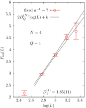
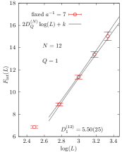
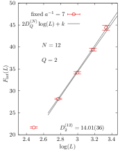
Figure 3: Estimation of UV scaling dimension $D^{(N)}_{Q}$ of the flux-$Q$ monopoles from the scaling of the lattice free energy $F_{\mathrm{lat}}(L)$ in $N$-flavor theory with box size $L$ at fixed small lattice spacing $\ell/L=1/7$. The panels show $F_{\mathrm{lat}}(L)$ as a function of $L$. The values of $(Q,N)$ in the panels from left to right correspond to $(1,4),(1,12),(2,4),(2,12)$ respectively. The data points are the lattice-determined values of $F_{\mathrm{lat}}$. The black bands are the $\log(L)$ fits to the data.

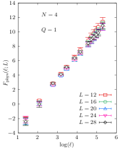
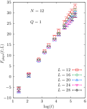
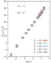
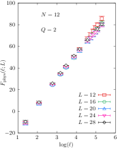
Figure 4: The free energy $F_{\mathrm{phys}}(\ell,L)$ converted to physical units is shown as a function of $\ell$. The data points at fixed $L$ are shown using the different colored symbols. The values of $(Q,N)$ in the panels from left to right correspond to $(1,4),(1,12),(2,4),(2,12)$ respectively.

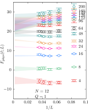
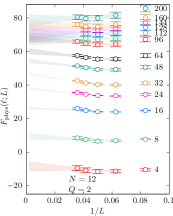
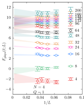
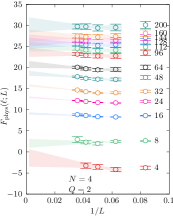
Figure 5: The continuum estimates of the $F_{\mathrm{phys}}(\ell)$ through $1/L$ extrapolations of $F_{\mathrm{phys}}(\ell;L)$ at different fixed physical box sizes $\ell$ noted beside the data points. The $1/L$ fits were made over the range $L\in[16,28]$. The bands show the extrapolations resulting from the fits. The values of $(Q,N)$ for the panels from left to right correspond to $(1,12),(2,12),(1,4),(2,4)$ respectively.

Using the determined $F_{\mathrm{lat}}(\ell;L)$ and the best fit values of $D_{Q}^{(N)}$ in the previous analysis, we obtained $F_{\mathrm{phys}}(\ell;L)$ as

$$F_{\mathrm{phys}}(\ell;L)=F_{\mathrm{lat}}(\ell;L)+2D_{Q}^{(N)}\log\left(\frac{\ell}{L}\right).$$ (17)

We propagated the statistical errors in $F_{\mathrm{lat}}(\ell;L)$ and the estimated $D_{Q}^{(N)}$ into the determination of $F_{\mathrm{phys}}$ by adding the errors in quadrature. In Figure 4, we show $F_{\mathrm{phys}}(\ell;L)$ as a function of $\log(\ell)$ for $Q=1,2$ in $N=4$ and 12 flavor theories. In each panel, we show the results of $F_{\mathrm{phys}}(\ell;L)$ from $L=12$, 16, 20, 24 and 28 together. First, we notice that $F_{\mathrm{phys}}(\ell)$ increases monotonically as we expected. Second, the lattice-to-physical units ‘renormalization factor’, $a^{-2D_{Q}^{(N)}}$ has caused a near data collapse of the $F_{\mathrm{phys}}(\ell;L)$ from multiple $L$. The residual $L$ dependencies at fixed $\ell$ need to be removed by extrapolating to $L\to\infty$ as we discuss below.

In Figure 5, we show the residual $1/L$ dependence of $F_{\mathrm{phys}}(\ell;L)$ for $Q=1$ and 2 monopoles in $N=4$ and 12 theories. The data points differentiated by their colors have a fixed value of $\ell$, and they have to be extrapolated to $L\to\infty$ to estimate the continuum limit $F_{\mathrm{phys}}(\ell)$ in that physical box size. We perform the extrapolation using a simple Ansatz, $F_{\mathrm{phys}}(\ell;L)=F_{\mathrm{phys}}(\ell)+k(\ell)/L$ with $F_{\mathrm{phys}}(\ell)$ and $k(\ell)$ fit parameters, to describe the $L$-dependence of $F_{\mathrm{phys}}(\ell;L)$ for $L\in[16,28]$. Such a fit was capable of describing the $L$-dependence well with $\chi^{2}/{\rm dof}<1$ in most cases. For $\ell=112,128,144$ in $N=12$ theory, we accidentally did not produce the $L=28$ lattice data. Therefore, we performed the extrapolation only using $L=16,20$ and 24 data sets in those specific cases resulting in a comparatively larger statistical error in their extrapolated values. The various colored bands in Figure 5 show the $1/L$ extrapolations at various fixed $\ell$. We will use the extrapolated $F_{\mathrm{phys}}(\ell)$ in the discussion of infrared dimensions of monopole operators in the next subsection.

III.2 Estimation of infrared scaling dimensions

First, we discuss the scaling dimensions in $N=12$ theory. Due to the relatively large value of $N$, this serves as a test case to see if the values obtained for the scaling dimension agree approximately with the large-$N$ expectations. In Figure 6, we show the dependence of $F_{\mathrm{phys}}(\ell)$ as a function of $\log(\ell)$ for the $N=12$ case. In the left and right panels, we show the $Q=1$ and $Q=2$ monopole free energies respectively. The black points in the panels are our estimates for the continuum limits of $F_{\mathrm{phys}}(\ell)$, as obtained in Figure 5. For comparison, we also show the data points for $F_{\mathrm{phys}}(\ell)$ from $L=24$ lattice before performing any continuum extrapolation. One expects a simple $\log(\ell)$ dependence only in the large-box limit, corresponding to large separations between the monopole and the antimonopole. Within the statistical errors, we see such a $\log(\ell)$ dependence for $\ell\geq 32$. We fitted

$$F_{\mathrm{phys}}(\ell)=f_{0}+2\Delta_{Q}^{(N)}\log(\ell),$$ (18)

using a constant $f_{0}$, and the infrared scaling dimension $\Delta_{Q}^{(N)}$ as fit parameters over two ranges $\ell\in[32,200]$ and $\ell\in[48,200]$ to check for systematic dependence on fit range. The underlying lattice data for $F_{\mathrm{lat}}$ are statistically independent at different $\ell$, but Eq. (17) introduces correlations between different $\ell$ due to the commonality of the second term in Eq. (17). We found the covariance matrix of the data for $F_{\mathrm{phys}}$ at different $\ell$ close to being singular making the minimization of correlated $\chi^{2}$ to be not practical, and we resorted to uncorrelated $\chi^{2}$ fits; this is an approximation made in this study. We determined the statistical errors in fit parameters using the Jack-knife method. For the $N=12$ theory under consideration, we determined $\Delta_{1}^{(12)}$ and $\Delta_{2}^{(12)}$ in this way. We show the resultant fits over $\ell\in[32,200]$ and $[48,200]$ as the blue and magenta error bands respectively in the two panels of Figure 6. The slopes of the $\log(\ell)$ behavior from the fits over $\ell\in[48,200]$ give

$$\Delta_{1}^{(12)}=2.81(66)\quad\text{and}\quad\Delta_{2}^{(12)}=8.2(1.0),$$ (19)

for $Q=1$ and $Q=2$ monopoles respectively. The $\chi^{2}/{\rm dof}$ for the two fits are 1.1/6 and 3.2/6 respectively, which are smaller than the typical value of around 1 due to the uncorrelated nature of the fit. By using a wider range of $\ell$ starting from a smaller $\ell=32$, we found $\Delta_{1}^{(12)}=2.91(41)$ and $\Delta_{2}^{(12)}=8.91(54)$ showing only a mild dependence on the fit range. The large-$N$ expectations Pufu (2014); Dyer et al. (2013) for these two scaling dimensions are $\Delta_{1}^{(12)}=3.1417$ and $\Delta_{2}^{(12)}=7.882$. We see that the estimates from the fit performed over $\ell\in[48,200]$ to be quite consistent with the large-$N$ expectation well within 1-$\sigma$ error. The more precise estimate of $\Delta_{2}^{(12)}$ from the fit over $\ell\in[32,200]$ is slightly higher than the large-$N$ value at the level of 2-$\sigma$, and is more probable to be a systematic effect from using the smaller $\ell=32$ in the fit rather than arise due to genuine higher $1/N$ corrections. It is reassuring that our numerical method obtains values for $\Delta_{Q}^{(12)}$ that are consistent with the large-$N$ expectations, which will add credence to the results from the method at smaller $N$ to be discussed next. As a minor note, by comparing to the slope of the red points, we see that continuum extrapolation at all $\ell$ was essential, without which we would have overestimated the values of $\Delta_{Q}^{(12)}$ by instead fitting the $\ell$ dependence at a fixed $L$.

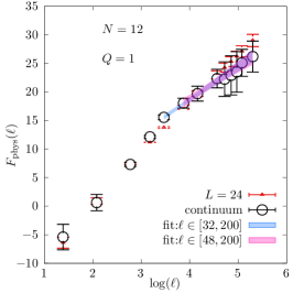
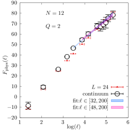
Figure 6: The physical free energy $F_{\mathrm{phys}}(\ell)$ in $N=12$ QED₃ is shown as a function of $\log(\ell)$ for $Q=1$ monopole in the left panel and $Q=2$ monopole in the right panel. The black points are the continuum estimates and the red points are from a fixed $L=24$. The blue and magenta bands are the $\log(\ell)$ fit over $\ell\in[32,200]$ and $[48,200]$ respectively.

Figure 7: (Left panel) The free energy $F_{\mathrm{phys}}$ is shown as a function of $\log(\ell)$ for $Q=1$ monopole in $N=4$ theory. The black points are the continuum estimates and the red points are from fixed $L=28$ lattice. The blue and magenta bands are the $\log(\ell)$ fit over $\ell\in[32,200]$ and $[48,200]$ respectively. The slopes of the fits give the scaling dimension $\Delta_{1}^{(4)}$. (Right panel) The difference from the expectation of the marginally relevant scaling with $\Delta_{c}=3$ is explored. The data points and the fitted bands in the left panel at larger $\ell$ are re-plotted as the difference, $F_{\mathrm{phys}}(\ell)-2\Delta_{c}\log(\ell)$. The horizontal dashed line is shown to compare the residual slope in the data.

First, we consider the $Q=1$ monopole in the $N=4$ theory. We looked at this case in our earlier work Karthik and Narayanan (2019b); the variation in the present study is the usage of higher statistics, differences in the sampled values of $\zeta$ to cover up to $\zeta=2$, and the incorporation of dedicated continuum limits at each fixed $\ell$ instead of using a simpler one-parameter characterization of $1/L$ effects at all $\ell$ used in the earlier work. In the left panel of Figure 7, we show the $\log(\ell)$ dependence of the free energy for $Q=1$ monopole in the $N=4$ theory. The black points are the continuum expectations, whereas the red ones are the data from the largest $L=28$ lattice. Again, we see a simple $\log(\ell)$ behavior is consistent with the data from boxes with $\ell\in[32,200]$. The fit to the functional form Eq. (18) over a range $\ell\in[48,200]$ gives a slope of

$$\Delta_{1}^{(4)}=1.28(26),$$ (20)

with a $\chi^{2}/{\rm dof}=1.2/6$. We show the resulting fit as the magenta error-band in Figure 7. This is consistent with the estimate $\Delta_{1}^{(4)}=1.25(9)$ from our earlier work. When we include the smaller $\ell=32$ in the fit (shown as a blue band), we find $\Delta_{1}^{(4)}=1.27(13)$ pointing to a very mild dependence on fit range. Clearly, $\Delta_{1}^{(4)}$ is smaller than the marginal value $\Delta_{c}=3$, which makes the $Q=1$ monopole operator relevant along the renormalization group flows of $N=4$ QED₃. We can see the relevance of $Q=1$ monopole operator without any fits by plotting the difference $F_{\mathrm{phys}}(\ell)-2\Delta_{c}\log(\ell)$. If the operator is relevant, we should see a negative slope in the above difference. Through a simple re-plotting of the data and fits in the left panel, we show the $\log(\ell)$ dependence of the difference, $F_{\mathrm{phys}}(\ell)-2\Delta_{c}\log(\ell)$, in the right panel. We see a clear negative slope in the data and reach the same conclusion about the relevance of $Q=1$ monopole in $N=4$ QED₃. This brings us to the main motivation for the present work; is the $Q=2$ monopole operator also relevant in $N=4$ QED₃?

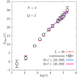
Figure 8: (Left panel) The free energy $F_{\mathrm{phys}}$ is shown as a function of $\log(\ell)$ for $Q=2$ monopole in $N=4$ theory. The black points are the continuum estimates and the red points are from fixed $L=28$ lattice. The blue and magenta bands are the $\log(\ell)$ fit over $\ell\in[32,200]$ and $[48,200]$ respectively. The slopes of the fits give the scaling dimension $\Delta_{2}^{(4)}$. (Right panel) The difference from the expectation of the marginally relevant scaling with $\Delta_{c}=3$ is explored. The data points and the fitted bands in the left panel at larger $\ell$ are re-plotted as the difference, $F_{\mathrm{phys}}(\ell)-2\Delta_{c}\log(\ell)$. The horizontal dashed line is shown to compare the residual slope in the data.

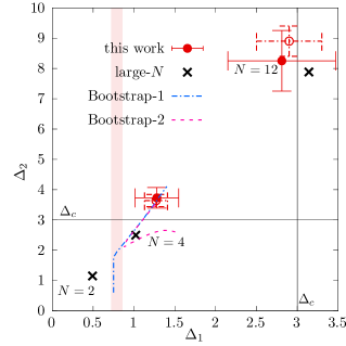
Figure 9: The scaling dimension of $Q=2$ monopole is plotted as a function of $Q=1$ monopole using their estimates for $N=2,4$ and 12 QED₃. The black crosses are the large-$N$ expectations. The filled red circles are the estimates in this paper obtained from finite-size scaling analysis of the data over $\ell\in[48,200]$. The open red circles are obtained by fitting the data over $\ell\in[32,200]$. The red vertical band is using the estimate of $\Delta^{(2)}_{1}$ from our earlier work. The two solid black lines indicate the critical value of $\Delta_{c}=3$ for the two scaling dimensions. The blue dot-dashed line (taken from Chester and Pufu (2016); Chester et al. (2018) labelled Bootstrap-1) and the magenta dashed line (taken from Albayrak et al. (2022) labelled Bootstrap-2) near the $N=4$ result are the boundaries separating the allowed and disallowed regions using conformal bootstrap methods for CFTs with infrared symmetry of $N=4$ QED₃. The region below the blue dot-dashed line and the region enclosed by the magenta line are the allowed regions according to the two studies respectively, each imposing certain choices of constraints on dimensions of operators occurring in the conformal expansion of monopole four-point correlators. The endpoints of the boundaries are simply the range shown in the two studies and not a hard cut-off.

In the left panel of Figure 8, we show the $\log(\ell)$ dependence of $F_{\mathrm{phys}}(\ell)$ for $Q=2$ monopole in $N=4$ QED₃. As in the previous cases we discussed, given the statistical errors, the finite-size dependence of $F_{\mathrm{phys}}(\ell)$ for $\ell\geq 32$ is consistent with a simple $\log(\ell)$ behavior. The magenta band shows the fit using such a $\log(\ell)$ fit in Eq. (18) to the data with $\ell\geq 48$. The value of the slope again gives the scaling dimension. From the best fit values, we estimate the scaling dimension of $Q=2$ monopole in $N=4$ QED₃ to be

$$\Delta_{2}^{(4)}=3.73(34),$$ (21)

with $\chi^{2}/{\rm dof}=1.4/6$. Thus, $\Delta_{2}^{(4)}>3$ with a weak statistical significance of about 2-$\sigma$. If we start the fit from a smaller $\ell=32$, we find a similar value $\Delta_{2}^{(4)}=3.65(21)$ with a smaller error. At $O(1/N)$ in the large-$N$ expansion, $\Delta_{2}^{(4)}=2.498$. Our data allows the possibility that either by the importance of higher $1/N$ orders in the large-$N$ expansion or by a breakdown of such an expansion for $N=4$, the value of $\Delta_{2}^{(4)}$ could be larger than 3, and make it irrelevant in the infrared. As we explained in the previous case of $Q=1$ monopole, to argue that the data is consistent with $\Delta_{2}^{(4)}>3$ without performing any fits, we re-plot the data as a difference $F_{\mathrm{phys}}(\ell)-2\Delta_{c}\log(\ell)$, where the second term corresponds to the expected slope at a marginal dimension $\Delta_{c}=3$. In the right panel of Figure 8, we show this difference over a range of larger $\ell$. In this plot, if the $Q=2$ monopole was relevant, one should see a $\log(\ell)$ dependence with a negative slope. The trend in the data indicates a positive slope, which again points to the consistency of our data with $Q=2$ monopole being irrelevant. As a final remark, we note that the behavior of $F_{\mathrm{phys}}(\ell)$ with $\Delta_{2}^{(4)}>3$ is not strongly dependent on the continuum extrapolation procedure. The red points in the two panels of Figure 8 are the free energies at different $\ell$ on the largest $L=28$ lattice. From the slope of the red points, we see that we would have reached an even stronger conclusion that $\Delta_{2}^{(4)}>3$ from that data alone. Therefore, the effect of $L\to\infty$ extrapolation has been to make that conclusion weaker.

We collect the results of $\Delta_{Q}^{(N)}$ in Figure 9. We plot $\Delta_{2}^{(N)}$ as a function of $\Delta_{1}^{(N)}$, making the dependence on $N$ implicit. The solid red points in Figure 9 are the values determined in this paper using fits over data from $\ell\in[48,200]$. To show the systematic artifacts in the estimate, we also show the estimates from fits over data from $\ell\in[32,200]$ as the open circles. In the previous work Karthik and Narayanan (2019b), we determined only the value of $\Delta_{1}^{(2)}$ in $N=2$ QED₃. Therefore, we show a red band in Figure 9 to indicate lack of data for $\Delta_{2}^{(2)}$. We show the large-$N$ expectation for $\Delta_{2}^{(N)}$ versus $\Delta_{1}^{(N)}$ as the black crosses. As we discussed before, the top-right red point from $N=12$ QED₃ is consistent with the large-$N$ expectation. The vertical and horizontal dashed lines in the figure indicate the marginal values of $\Delta_{1}=3$ and $\Delta_{2}=3$ respectively. The data point from $N=12$ lies at the edge of $\Delta_{1}=3$, which indicates that $N=12$ QED₃ is close to being the critical flavor below which $Q=1$ monopole becomes irrelevant. As pointed out in Pufu (2014), one could conjecture that the critical flavor that separates the mass-gapped and conformal infrared phases of $N$-flavor compact QED₃, where all flux-$Q$ monopoles can freely arise, is around $N\approx 12$. The important finding in this paper is that the $N=4$ data point in Figure 9 lies above the critical horizontal line, albeit with a weaker statistical significance of about 2-$\sigma$ (or 3-$\sigma$ if one bases the conclusion on the red open point). We also see that the estimated location of the $N=4$ data point in the plot is quite robust with respect to change to the fitted range of $\ell$. Thus, our data cannot rule out the scenario where $Q=2$ monopole remains irrelevant along the renormalization group flow even for the $N=4$ theory. For comparison, we also show the boundary of the allowed region in the $\Delta_{1}-\Delta_{2}$ plane for CFTs that have the symmetries of $N=4$ QED₃ as determined using the conformal bootstrap approach. The blue dot-dashed line is the boundary computed in Refs Chester and Pufu (2016); Chester et al. (2018), and the region below the line is allowed. The magenta dashed line is the boundary computed in Ref Albayrak et al. (2022) with the allowed region enclosed by the curve. In both cases, we obtained the data from the plots as shown in the two papers and the region covered in the $\Delta_{1}-\Delta_{2}$ plane is only representative of the region shown in the two studies and not a hard cut-off . In both the bootstrap studies, there exists an allowed region where $\Delta_{2}>3$. The data point for $N=4$ case from our lattice study is quite consistent with this allowed region within errors, and the central value conspicuously sits right at the allowed upper boundary line in the two studies. It would be interesting to fold in this finding as an input for future conformal bootstrap studies.

IV Conclusions

Along with the composite operators such as fermion bilinears and four-Fermi operators, monopole operators that introduce $2\pi Q$ fluxes around their insertion point constitute nontrivial insertions in QED₃. The motivation for this study was the question of infrared relevance of the $Q=2$ monopole operators in QED₃ coupled to massless $N=4$ Dirac fermion flavors. We used numerical lattice simulations of noncompact QED₃ coupled to $N=4$ and $N=12$ flavors of Wilson-Dirac fermions fine-tuned to the massless point. We estimated the infrared scaling dimensions of $Q=1$ and $Q=2$ monopoles in the $N=4$ and 12 theories from the finite-size scaling analysis of free energy required to introduce the $Q=1$ and 2 monopole-antimonopole pairs in the two theories. We validated the method in $N=12$ theory first where the values of the $Q=1$ and 2 scaling dimensions would be expected to lie closer to the values obtained from the first-order large-$N$ expansion. Then, by applying to the $N=4$ theory, we found our best estimate for $Q=2$ scaling dimension to $3.73(34)$, which is consistent with being greater than the marginal value of $3$. Thus, our result favors, and certainly cannot rule out, the possibility of $Q=2$ monopole operators being irrelevant at the infrared fixed point of $N=4$ QED₃. We summarized our results for the scaling dimensions in Figure 9 that shows the dimension of $Q=2$ monopole as a function of the dimension of $Q=1$ monopole, and we compared it to determinations from conformal bootstrap.

As argued in Refs Song et al. (2020, 2019), the irrelevance of $Q=2$ monopole operators at the infrared fixed point of $N=4$ noncompact QED₃ could imply the possibility of hosting a stable U(1) Dirac spin liquid phase in non-bipartite lattices, such as on the triangular and Kagomé lattice. On such lattices, it has been argued Song et al. (2020, 2020) that the $Q=1$ monopoles are disallowed due to symmetry reasons, and the most important destabilizing perturbation could be that of the next allowed higher-flux monopole, which is the $Q=2$ monopole on the Kagomé lattice. The findings from our numerical study mildly support the exciting possibility that the higher-flux monopoles might not destabilize the Dirac spin liquid on such non-bipartite lattices.