Confinement-driven state transition and bistability in schooling fish

Abstract

We investigate the impact of confinement density (i.e the number of individuals in a group per unit area of available space) on transitions from polarized to milling state, using groups of rummy-nose tetrafish (Hemigrammus rhodostomus) under controlled experimental conditions. We demonstrate for the first time a continuous state transition controlled by confinement density in a group of live animals. During this transition, the school exhibits a bistable state, wherein both polarization and milling states coexist, with the group randomly alternating between them. A simple two-state Markov process describes the observed transition remarkably well. Importantly, the confinement density influences the statistics of this bistability, shaping the distribution of transition times between states. Our findings suggest that confinement plays a crucial role in state transitions for moving animal groups, and, more generally, they constitute a solid experimental benchmark for active matter models of macroscopic, self-propelled, confined agents.

I Introduction

A remarkable feature of assemblies of living organisms is their ability to continuously adapt to constraints from their environment. In many species, this ability is manifested through collective motion, where a group can form very characteristic spatial structures, also known as collective states. While a large variety of such structures exists in the wild, studies on collective motion usually suggest that the different collective states can be classified into 3 distinct families [1]: swarming, a disorganised state in which the orientations (directions of displacement) within the group are essentially isotropic; a polarized state, in which members of the group move in a preferential direction while being aligned with each other; and milling, a state where individuals move forming a vortex-like structure, rotating as a whole around the centre of mass of the group. The transition to this milling state is widespread and has been extensively described for a number of different species: marine worms [2], planktonic crustaceans [3], army ants [4], reindeers [5] and most notably in fish [6, 7, 8, 9]. In some groups of animals, this milling structure is part of a multi-stable regime, where the system switches between several states, depending on the experimental conditions [10, 11].

Collective motion confers a variety of advantages to the group, which may exceed the capabilities of lone individuals. Therefore, from an evolutionary standpoint, this emergent behavior is encouraged. These benefits range from improved predator avoidance and escape [12, 13, 14]to a reduced cost of locomotion [15, 16, 17].

Previous studies have often focused on deciphering the interactions between individuals that lead to a given stable collective state. However, the fluctuating essence of natural environments means that these groups must be able to shift their structure based on external stimuli and constraints [18]. Understanding the underlying mechanisms of such structural transitions is thus of high interest to be able to describe complex biological systems.

Numerous physical parameters are able to trigger state transitions in groups of moving organisms by altering the nature or intensity of the inter-individual interactions, such as light intensity [3, 19, 20] or noise [21]. The existing numerical models of self-propelled particles (SPP) also indicate that one of the key factors explaining these transitions is the density of the group [3, 22, 23, 24]. For fish schools specifically, studies have highlighted density-driven transitions, either experimentally [25, 26] or with numerical simulations [27, 28]. These studies primarily investigate the role of the school size, while also noting that the proximity to walls can play a crucial role in triggering specific transitions, like the milling to polarization transition [26].

We can unify these observations by examining the issue of state transition from the perspective of group confinement –in the sense of how crowded the available area is– which covers two distinct factors: the number of individuals in the group, and the surface of the swimming arena. The impact of confinement and the effect of boundaries have been previously studied for systems of non-living [29] or microscopic active matter (from bacteria [30, 31] to cells [32]), but seems to be a missing ingredient in our current understanding of state transitions for groups of live animals. The study by [26] indicates that the swimming area is not significant in the state transitions between swarming, milling, and polarized states in groups of golden shiners. However, this conclusion was based on a single experiment carried out for a different swimming area. As of yet, no study has systematically investigated how confinement, both in terms of the number of individuals and the arena surface, impacts groups of animals on the move. Notably, the link between confinement and behavioral state transitions remains unsettled.

Here we report quantitative results on the collective dynamics of groups of rummy-nose tetras (Hemigrammus rhodostomus), a highly cohesive fresh water fish, under controlled experimental conditions. In first approximation, if one neglects the exact shape of the tank, the notion of confinement can be simply quantified by a ”confinement density” $\rho$, which is the number of fish per unit area of the tank. Our analysis provides novel experimental evidence for a continuous state transition governed by confinement density. During this transition, the school experiences a bistable state, in which both polarization and milling states coexist; the group can fall randomly into one of these two states. Bouts of variable durations of either state intercede one another alternately over time. By measuring the distribution of transition times between states, we show that the statistics of this bistability is also directly influenced by the confinement density. Through these results, we show that the presence of walls and the group size play a comparable role in the emergence of collective dynamics in schooling fish.

II Material and Methods

The experiment consists of recording the motion of free-swimming schools of Hemigrammus rhodostomus in a tank, using the same setup as described in [19], for different swimming areas $S$ and school sizes $N$ (number of individuals in the group). We systematically investigated the role of the confinement density, or mean density, $\rho$, defined as the ratio of these two values $\rho=N/S$ in fish/m². The water depth in the tank is sufficiently shallow (6 cm) to constrain the trajectories in two dimensions. The average body length (BL) of the fish used here is 32 mm (See Supplemental Material Sections III, IV and V ).

The swimming area can be modified by a system of movable partition walls. Three different surfaces are considered: 1, 0.5 and 0.25 m². We focus mainly on arenas with a square shape (aspect ratio $AR$ = 1), but we briefly discuss the implications of a different aspect ratio. We studied 10 different group sizes ranging from 10 to 70 fish, resulting in densities between 10 and 120 fish/m². During the experiments, the tank is brightly lit from above with visible light (900 lux) and back lit with an infrared LED panel to enhance the contrast of the images captured by the camera (Figure 1a-b). The acquisition frequency of the camera is 50 frames per second ($\Delta t=0.02$ s).

Using the open source particle tracking library Trackpy [34, 35], we extract the temporal signals of the two-dimensional positions $\mathbf{x}_{i}(t)$, from which we obtain velocities with a second order central differences method $\mathbf{v}_{i}(t)=[\mathbf{x}_{i}(t+\Delta t)-\mathbf{x}_{i}(t-\Delta t)]/2\Delta t$, where $i=1,2,...,N$ is the fish label (See Supplemental Material Section VI for details on the tracking accuracy ).

For each confinement density, at least 2 different pairs of values of $N$ and $S$ corresponding to that density were tested (except for the two extreme density values 10 and 120 fish/m²). We conducted at least 3 different trials of 15 min for every pair of values (swimming area, school size). In total, 76 distinct experiments have been conducted.

We use the canonical milling and polarization parameters ($\mathcal{M}$ and $\mathcal{P}$) to capture the collective dynamics at the group level:

$$\mathcal{M}=\frac{1}{N}\left|\sum_{i=1}^{N}\tilde{\mathbf{r}}_{i}\times\tilde{\mathbf{v}}_{i}\right|$$ (1)

$$\mathcal{P}=\frac{1}{N}\left|\sum_{i=1}^{N}\tilde{\mathbf{v}}_{i}\right|$$ (2)

where $r_{i}$ is the position of the $i$-th fish with respect to the school’s center of mass ($\mathbf{r}_{i}=\mathbf{x}_{i}-1/N\sum_{i=1}^{N}\mathbf{x}_{i}$), and $\tilde{\cdot}$ is the normalization operator ($\tilde{\mathbf{u}}=\mathbf{u}/|\mathbf{u}|$).

These parameters allow the structure of the school to be described mathematically, highlighting the typical states discussed above. When $\mathcal{M}$ is large (close to 1) and $\mathcal{P}$ is small (close to 0), the group is in the milling state; conversely, when $\mathcal{M}$ is small and $\mathcal{P}$ is large, the fish are in the polarized state. Figure 1a-b provides examples of these characteristic schooling states in our experimental setup.

III Results

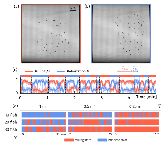
Figure 1: Example of an experimental result for $N=50$ fish schooling in a square tank of swimming area $S=1$ m². Snapshot of the school in (a) milling configuration ($\mathcal{M}\approx 1$) and in (b) polarized configuration ($\mathcal{P}\approx 1$). The photographs show the entire surface of the tank. (c) The time signal of $\mathcal{M}$ and $\mathcal{P}$ shows clearly distinct periods of milling state followed by periods of polarized state of respective duration $\tau_{\mathrm{m}}$ and $\tau_{\mathrm{p}}$. The colored bar represents the current state of the school. (d) State transitions over 15 min experiments for various school sizes $N$ and swimming area $S$.

The experiment consists in recording the motion of free-swimming schools of Hemigrammus rhodostomus in a tank, using the same setup as described in [19], for different swimming areas $S$ and school sizes $N$ (number of individuals in the group). When qualitatively examining the dynamics of the fish at the different combinations of $N$ and $S$, we see that the group of tetras spontaneously and repeatedly alternate between milling and polarized states as can clearly be seen in Figure 1c. We also note that the characteristic length of the group evolves as the square root of the number of fish $N$, regardless of the swimming area $S$ considered. This suggests that the local density (density for which the area considered is not the available swimming area $S$ but only the surface area occupied by the school) is maintained for all the experiments carried out, here at around 180 fish/m² (See Supplemental Material Section I for details on the local density).

At the smallest density values (10-20 fish/m²), we observe that the school remains in a polarized state for almost the entire recording duration, with only short-lived (a few seconds) incursions to the milling state that quickly revert to the polarized state. This behavior is illustrated in Figure 1d, for $S=1$ m² and $N=10$. As we further increase the confinement density by adding more fish to the school or reducing the swimming area (typically for densities between 20 and 80 fish/m²), the bistability can be more clearly observed, as milling bouts last for longer. The group state shows an increase in fluctuations, with frequent shifts observed between the polarized and milling states, although the proportion of time in the polarized state remains more significant than the time spent in the milling state for densities lower than 40 fish/m²; as the density increases again, the milling state becomes more predominant (see Figure 1d, for $S=0.5$ m² for example). Finally, when approaching densities of 100 fish/m² and above, the groups mostly display a milling behaviour that lasts for long durations of time, still punctuated with occasional very short periods of polarization (typically less than a few seconds). This is shown by the panel corresponding to $S=0.25$ m² and $N=30$ in Figure 1d.

This bistability of the school has been observed previously in experimental [26] and numerical studies [10, 11], and is reminiscent of a simple dynamical system oscillating between two stable states. This leads us to define these two states objectively: we say that the school is in the milling state (resp. in the polarized state) when $\mathcal{M}>0.5$ (resp. when $\mathcal{P}>0.5$). The colored bar above the time signal in Figure 1c shows that the two states follow each other almost without interruption. Inspired by thermodynamics [37], the bistability of the fish group can be described by a potential landscape: transitions take place when the fluctuations of the system are greater than the corresponding potential barrier.

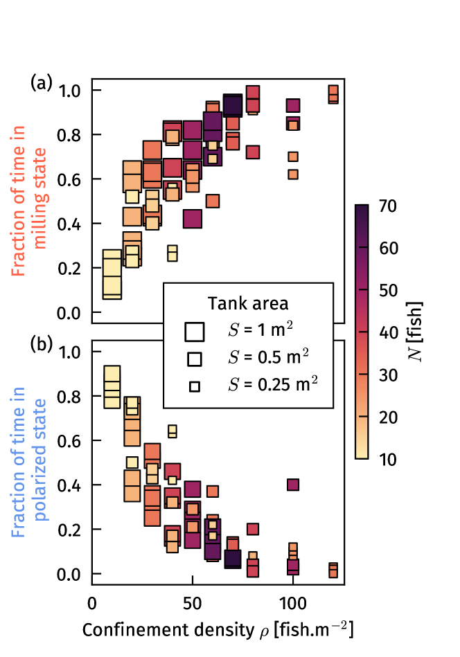
Figure 2: Fraction of time spend by fish schools in the milling state (a) and in the polarized state (b) over total experiment duration, with respect to confinement density, i.e the number of fish per unit area of the tank in fish.m^-2. The size of the markers indicates the area of the tank, while the colors show number of fish in the school.

In order to quantify the observed intermittency in states we first investigate it on the time scale of each experiment (15 minutes). Figure 2 shows the time spent in either state plotted as a function of confinement density $\rho$. First, it corroborates the observations made on individual experiments, where time spent milling goes up with the density, and oppositely for time spent in the polarized state. Most strikingly Figure 2 shows a clear collapse of the data of a total of 76 experiments with 20 different ($N,S$) combinations when plotted against the confinement density. For each confinement density (with the exception of 10 and 120 fish/m^-2), experiments with at least two ($N,S$) combinations were carried out, to ensure that they yielded equivalent results if the $N/S$ ratio was the same. This collapse clearly highlights that the proportion of time spent by the group of Rummy-nose tetras in either state is solely a function of the confinement density, rather than of the number of fish alone, as suggested by previous studies on golden shiners [26].

We introduce a simple two-state Markov process at the scale of the school to gain insight on the transition between the polarized and milling states. In this scenario, the school is considered as a bistable system; we denote $\alpha$ (resp. $\beta$) the rate of transition from the polarized to milling states (resp. from milling to polarized). The transition probability from polarized to milling (resp. milling to polarized) during a time $\delta t$ is therefore $\delta t\alpha$ (resp. $\delta t\beta$). This probability is considered to depend only on the current state and is independent of the history of the system. In this case, the time between switching events (i.e the duration of the bout spent in either state) follows a Poisson distribution with a rate parameter specific to that state. We have the following probability density functions for the duration of milling and polarized bouts:

$$\mu_{\mathrm{p}}(\tau_{\mathrm{p}}=\tau)=\alpha\exp(-\alpha\tau)$$ (3)

$$\mu_{\mathrm{m}}(\tau_{\mathrm{m}}=\tau)=\beta\exp(-\beta\tau)$$ (4)

We experimentally measured the time spent in the milling and polarized states. The results, reported in Figure 3a-b show an exemple of the empirical distribution of the durations between state transitions, for a confinement density at which fish spend approximately the same time in the milling and polarized states ($\rho=30$ fish/m², for $N=30$ and $S=1$ m²). At low densities, where transitions are frequent and the experimental statistics is therefore good, fitting an exponential distribution to the data shows good agreement. It should be noted that as density rises, and milling bouts become very long, the number of transitions falls sharply, and the number of bouts observed is much lower. For these high densities, the fit quality deteriorates, likely due to the insufficient statistics behind the experimental distribution. From the fit parameters we can directly obtain the mean time to transition for each state, with $\langle\tau_{\mathrm{m}}\rangle=\beta^{-1}$ and $\langle\tau_{\mathrm{p}}\rangle=\alpha^{-1}$. The good agreement demonstrated by the distributions in Figure 2a-b, which closely fit to an exponential distribution is the hallmark of a memory-less process and suggests that the school operates as a system near a pseudo-critical point [38, 18].

With this approach we extract $\alpha$ and $\beta$ for every set of experiments, that is for all pairs of ($N$, $S$). The variations of the two rates are presented on Figure 3c, with respect to the confinement density. We see that the stability of the milling state increases with density, while that of the polarized state decreases.

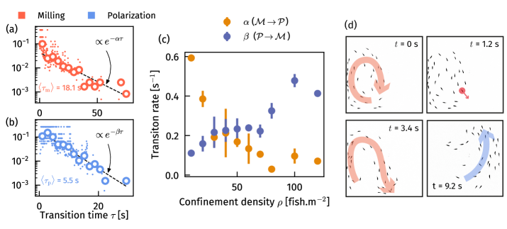
Figure 3: Probability density function of the duration of milling state $\tau_{\mathrm{m}}$ (a) and polarized state $\tau_{\mathrm{p}}$ (b) for a confinement density $\rho=30$ fish/m² ($N=30$, $S=1$ m², 6 replicates, 387 transition events). Small dots are generated by differentiating the complementary cumulative density function obtained from sorting the transition times, they do not depend on the binning. Large points are histograms obtained by binning data into 15 linearly spaced time intervals. Dashed lines show the best exponential law fit with parameter $\alpha=\langle\tau_{\mathrm{m}}\rangle^{-1}$ and $\beta=\langle\tau_{\mathrm{p}}\rangle^{-1}$ (c) Transition rates with respect to confinement density. Error bars represent the standard deviation. (d) Experimental snapshots of 40 fish in a 1m² tank illustrating the mechanisms underlying a transition from milling to polarized state. The black borders represent the tank walls.

When considering this two-state description of the group of tetras, one can look into the mechanisms that lead the system to switch from one to the other. From the bistability studied in our experiments, we can take away a few qualitative observations. The polarization to milling transition seems to be the consequence of the front of the polarized group seeing its back and, like a snake biting its tail, switches to a ’circular chase’. The mechanism of the milling to polarization transition is less obvious, but appears to be caused by the behavior of one individual straying away from the mill and entraining the rest of the group leading to the breaking of the mill. This observation is a qualitative confirmation of previous numerical simulations by Calovi et al. [39]. This mechanism is illustrated in Figure 3d.

IV Discussion

In this study, density variations are carried out at a constant aspect ratio $AR$, for square-shaped tanks ($AR$=1). However, since wall interaction was found to play a dominant role in the observed collective state transitions, a series of additional qualitative experiments at different $AR$ is conducted. We observe that, starting from a situation where milling is predominant at $AR=1$, it disappears and is replaced by polarization as $AR$ increases, i.e. for increasingly elongated tanks. This behavior points interestingly to the fact that, in addition to confinement density, the shape of the tank plays a non-negligible role in the milling-polarization transition described here. This could explain previous experimental results that seem contradictory [26], where milling decreases with increasing density, but where the ratio aspect is not preserved (a detailed description and complete interpretation of this additional dataset are reported in Supplemental Material Section II).

Although in this work, the confinement of the group of fish is carried out using simple walls, analogies can be drawn with systems in the wild. Confinement in cases of predation can take different forms: in some cases real boundaries are introduced, as with humpback whales caging off schools of fish, trapping them [40], in others the boundary may be effective like with dusky dolphins herding fish into ’prey balls’ [41]. Although these analogies are mostly qualitative, the parallel one can draw between geometric confinement and predation pressure opens an interesting avenue for research. Better understanding these similarities can help us break down complex behaviors observed in the wild.

The experiments reported here constitute the first quantitative laboratory study of the influence of confinement on the social behavior of live animals. Along with the works previously reported by [19], the results described above demonstrate that the collective states depend both on interactions between individuals and the environment of the fish group. Fundamentally, the coupling between the collective state and the surroundings is unsurprising, as the evolutionary pressure that has given rise to these states is likely highly environment-dependent.

In the case of confinement, we showed here that the nature of the bistability between polarization and milling of the group of Hemigrammus rhodostomus was controlled by confinement density. Whether it be the overall proportion of time spent in either state, or the statistical nature of bout durations, the intensity of the confinement seems to play a pivotal role. Furthermore, the qualitative investigation of different aspect ratios has shown that the boundary conditions can remove the bistability and select either state. These experimental results can be useful for future numerical models or the development of theory as an empirical benchmark to which these could be compared.

The confinement-driven state transition evidenced here, and the description of a group on the move as a bistable system, paves the way to examining other systems, biological or robotic, where the environment and boundary conditions will impose a confinement.

Supplemental Materials: Confinement-driven state transition and bistability in schooling fish

I Evolution of school area with confinement

In order to assess the local density of the group, we use tracking data to evaluate the temporal evolution of the surface area occupied by the school. To do this, the area of the convex hull of the school $A$ is determined at each time step. This is the area of the smallest convex surface containing all the points $\mathbf{x}_{i}$ for $i\in 1\dots N$, i.e. the positions of the fish in 2D. The variations of $A$ (averaged over the duration of the experiments) are shown in Figure S1 as a function of the experimental parameters.

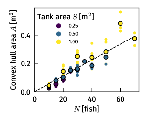
Figure S1: Area of the convex hull of the school $A$, averaged over the duration of the experiments, expressed in m². The colors represent the different swimming areas $S$ and the dashed line is the best linear fit for all the data. Small dots represent unique experiments and large points are average over the replicates.

Figure S1 shows the values of $A$ with respect to the number of fish in the school $N$, for the 3 different swimming areas $S$. The first observation is that variations of $S$ have no influence on the school area, and that the school area increases slowly with $N$. We fit the experimental data with a linear function, tanks to a least squares method:

$$A=S_{0}N$$ (S1)

with $S_{0}$ a constant fitting parameter homogeneous to a surface. The evolution of $A$ is well captured by this fit, which suggests that whatever the experimental conditions, we can consider that the fish school maintains a constant local density. The best fitting parameter value is found to be $S_{0}=3.67\pm 1.13\,\text{ BL}^{2}$: this surface can be interpreted as a minimal comfort area maintained by each individual around itself. This can also be understood in the following way: the local density is conserved, and is on average 179 fish/m².

II Role of the aspect ratio $AR$ of the tank

To assess the influence of the aspect ratio of the swimming tank $AR$ on the transition between polarized and milling sates, we conducted additional qualitative experiments with different $AR$ values, specifically $AR$ = {1, 2, 4, 10}. In this series of experiments, the length of the tank remains fixed at 1 m, while its width is varied to 50, 25, and 10 cm, respectively. All other experimental parameters, such as frame rate, water depth, and ambient light intensity, were kept consistent with the conditions used in the initial set of experiments. This additional dataset consists of one video recording of 10 minutes of schooling for each value of $AR$. Because of the proximity imposed on the fish in this setup (especially at high $AR$), trajectory crossings are common and periods where fish are superimposed are regularly observed; therefore, tracking accuracy drops drastically and renders quantitative analysis with the tracking pipeline used for this study unreliable. However, a qualitative analysis of collective behaviour is still possible from the raw images.

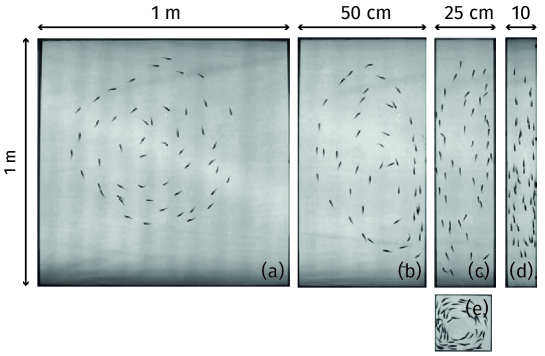
Figure S2: Effect of a variation of the aspect ratio $AR$ of the tank, from $AR=1$ to $AR=10$. The height of the swimming area remains fixed at 1 m while its width changes: (a) 1 m (b) 0.50 m (c) 0.25 m (d) 0.1 m. Panel (e) shows an experiment in a 0.2 m $\times$ 0.2 m ($AR=1$). Note that the milling motion is totally suppressed for $AR>2$.

As shown in Figure S2a-d, milling is clearly suppressed for elongated tanks with aspect ratios greater than 2. Starting from a situation where milling exists approximately 60% of the time in a square tank, we see a reduction in the time spent milling and a deformation of the vortex structure formed by the fish when we move to an aspect ratio of 2. Beyond $AR$ = 2, the milling almost no longer exists (no longer at all for $AR=10$), and the fish move back and forth between the two ends of the tank, remaining aligned along its long side. We note that in this case the transition is exclusively due to geometric constraints, since at the confinement density considered here (respectively 100, 200, 500 fish/m² for $AR=$ 2, 4, 10), we are well above the threshold after which we observe only milling in the case of a square tank. It is also interesting to point out that, starting from a situation where the milling is suppressed (for example the tank with an aspect ratio of 4), it is still possible to make the milling ’reappear’ by reducing the aspect ratio, as demonstrated by an additional experiment carried out in a 20 by 20 cm square tank (see Figure S2e).

We hypothesize that these observations explain the experimental results obtained by Tunström et al. [26]: they reported that, when reducing the swimming area, higher confinement density does not lead to increased time spent milling. However, this reduction of area was conducted at an aspect ratio of approximately 2 (66 $\times$ 38 cm), which means that they might have observed the same phenomenon of geometrical suppression of milling that we describe here.

III Experimental setup

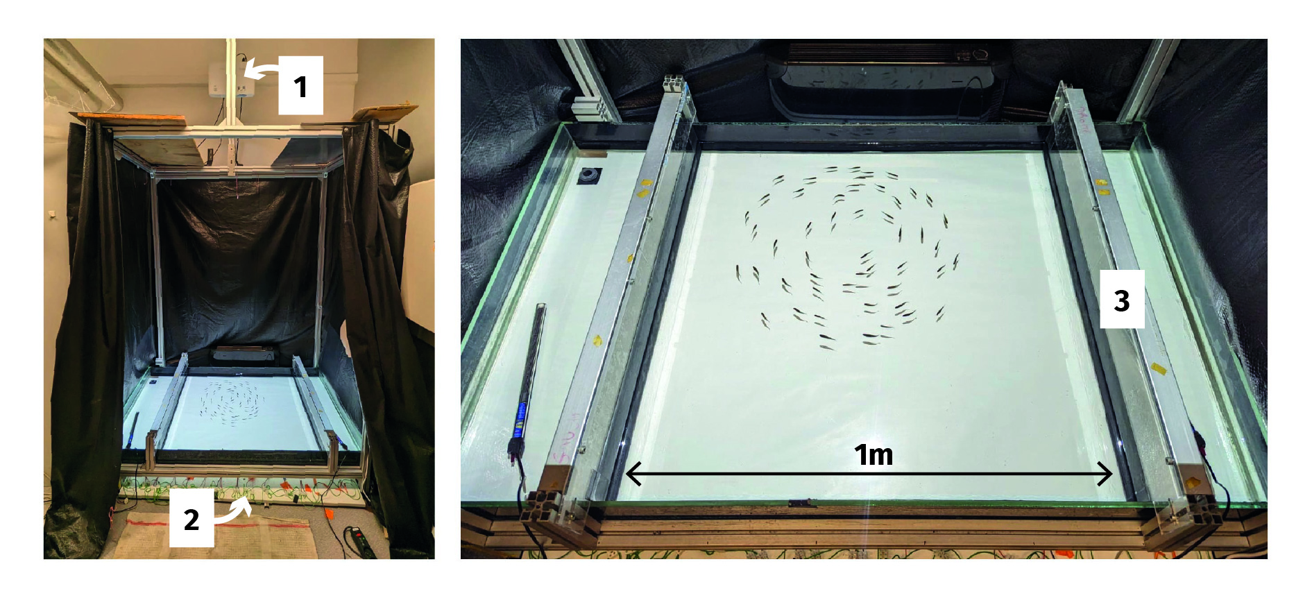
Figure S3: Experimental setup. (1) Videoprojector used to set the ambient light intensity. (2) Infrared LED pannel used as a back lighting. (3) Mobile partition walls to set the swimming area.

The experimental setup is a shallow water tank (100 cm $\times$ 140 cm) with mobile partition walls used to modify the swimming area (Figure S3-3). For surfaces of 0.5 m² and 0.25 m², a third partition wall is added so that the shape of the tank remains a square, with respective height 68$\pm 2$ cm and 50$\pm$2 cm. A videoprojector pointing down is attached at a height of approximately 250 cm. It controls the ambient light intensity by projecting still white images. For all the experiments presented in the article, the illumination is fixed at 900 lux. Below the tank we place a powerfull custom-made infrared LED pannel ($\lambda=890$ nm) that allows for high-contrast imaging in any visible light condition, without perturbation for the fish. A Basler camera (4 Mpx, not visible in the picture) is placed at 300 cm above the water surface, with a visible light filter in front of its objective (letting only infrared light with wavelengths larger than 920 nm pass through) to avoid perturbation from visible light sources in the room.

IV List of experiments

A list of all the experiments whose data were used in the main text is given in Figure S4.

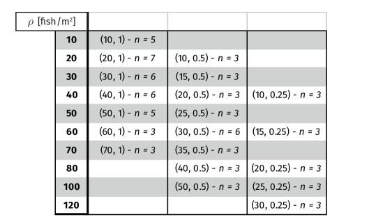
Figure S4: List of the experiments carried out for each pair of parameter (number of fish, swimming area [m²]); $n$ is the number of replicates of the same experiment, with a different group of fish.

V Experimental procedure

V.1 Fish Breeding

Rummy-nose tetra (Hemigrammus rhodostomus, BL = $3.92\pm 0.42$ cm) were bought from a professional supplier (EFV group, http://www.efvnet.net). Fish were kept in a 120 L tank on a 14:10 h photoperiod (day:night), similar to that existing at their latitudes of origin. The water temperature was maintained at 27°C($\pm$1°C) and fish were fed ad libitum with fine pellets from an automated feeder once a day, at a fixed time in the morning. The fish handling protocol complies with the European Directive 2010/63/EU for the protection of animals used for scientific purposes, as certified by the ESPCI Paris Ethics Committee

V.2 Experiments

Fish are manually counted and transferred from their aquarium to the observation tank. Manual count of the fish sometimes leads to a small error in fish count, in particular when the total number is high: therefore, for values of $N$ higher than 30, the stated value of $N$ for an experience should be considered with a $\pm 1$ uncertainty. The fish tank is curtained off, so that the light intensity projected (900 lux) is constant from one experience to another. Before starting the experiment, the fish are given 10 minutes with the no illumination to wear off stress caused by the tank change. The experiment is then carried out and lasts 15 minutes. Experiments can be repeated up to 3 times with 10 minute rest intervals where the projector is switched off. Fish are then given a period of at least 24h to rest between two experiment sessions.

Note that for the smallest values of swimming area, we did not carry out trials with large numbers of fish, as this would have resulted in excessively high densities, which could have been stressful for the animals. On the other hand, we could not reach values of density of density lower than 10 fish/m² because we have chosen to restrict ourselves to a number of individuals greater than 10, as it is uncertain whether the interactions are similar in a case where very few individuals interact.

VI Data Processing

VI.1 Fish tracking

Experiments are filmed at 50 frames per second and then analyzed using the Python library Trackpy [34, 35] which returns the positions $\mathbf{x}_{i}(t)$ of detected fish at each frame and connects the points on different frames to form trajectories. The position function of each fish is then filtered with a Savitzky-Golay filter of order 2 (window of 21 frames, which is approx. 0.4 s at 50 frames par second). The filtered signal is then derivated to obtain the velocities $\mathbf{v}_{i}(t)$ of the fish with a second order central differences method:

$$\mathbf{v}_{i}(t)=\frac{\mathbf{x}_{i}(t+\Delta t)-\mathbf{x}_{i}(t-\Delta t)}{2\Delta t}$$

with $\Delta t=0.02$ s is the acquisition period.

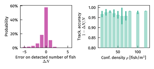
Figure S5: (left) Distribution of the error on the number of fish detected by the tracking algorithm $\Delta N$ (for all the frames in all the experiments). (right) Tracking accuracy -ratio between number of detected fish and fish present in the tank- for the different confinement densities $\rho$ tested in this study. The error bars represent the standard deviation over the different experiements at a given $\rho$.

The quality of tracking is assessed using two metrics: the error in the number of fish detected $\Delta N$, and tracking accuracy, which is the ratio between the number of fish detected $N-\Delta N$ and the actual number of fish in the tank $N$. Figure S5 shows the results of the tracking quality evaluation. The left-hand panel on Figure S5 shows the distribution of the error on the number of fish detected, for all frames of all experiments. It can be seen that all fish present are detected 58% of the time, and that the absolute error on $N$ is less than 1 88% of the time. Moreover, the distribution is restricted to values ranging from -5 to 5. The right-hand panel on Figure S5 shows the tracking accuracy, which is a measure of the proportion of fish detected relative to the total number of fish, as a function of the different confinement densities $\rho$ tested. We can see that for all $\rho$, tracking accuracy remains above 0.95, i.e. whatever the experimental parameters, 95% of the fish present are detected.

VI.2 Time series processing

Once the trajectories have been obtained using tracking, the temporal signals of the order parameters $\mathcal{M}(t)$ and $\mathcal{P}(t)$ are computed. To assess the behavioural state of the school (milling or polarized), these time signals are filtered using a Gaussian filter with parameter $\sigma$ = 16. In this way, the information contained in the signals is smoothed over a characteristic duration of approximately 1 s (3 $\times$ 16 = 48 frames, for an acquisition at 50 fps). This time scale represents a compromise, which makes it possible to reduce the noise present in the order parameter signals while losing a minimum of information, since the transition times are typically much greater than 1 second.

References

- Calovi et al. [2014a] D. S. Calovi, U. Lopez, P. Schuhmacher, H. Chaté, C. Sire, and G. Theraulaz, Journal of the Royal Society Interface (2014a), 10.1098/rsif.2014.1362.
- Franks et al. [2016] N. R. Franks, A. Worley, K. A. J. Grant, A. R. Gorman, V. Vizard, H. Plackett, C. Doran, M. L. Gamble, M. C. Stumpe, and A. B. Sendova-Franks, Proceedings of the Royal Society B: Biological Sciences (2016), 10.1098/rspb.2015.2946.
- Ordemann et al. [2003] A. Ordemann, G. Balazsi, and F. Moss, Physica A: Statistical Mechanics and its Applications Stochastic Systems: From Randomness to Complexity (2003), 10.1016/S0378-4371(03)00204-8.
- Schneirla [1944] T. C. Schneirla, (1944).
- Espmark and Kinderås [2002] Y. Espmark and K. Kinderås, Rangifer (2002), 10.7557/2.22.1.687.
- Harvey-Clark et al. [1999] CJ. Harvey-Clark, WT. Stobo, E. Helle, and M. Mattson, Copeia (1999), 10.2307/1447614.
- Couzin et al. [2002] I. D. Couzin, J. Krause, R. James, G. D. Ruxton, and N. R. Franks, Journal of Theoretical Biology (2002), 10.1006/jtbi.2002.3065.
- Wilson [2004] S. G. Wilson, Fisheries Oceanography (2004), 10.1111/j.1365-2419.2004.00292.x.
- Lukeman et al. [2009] R. Lukeman, Y.-X. Li, and L. Edelstein-Keshet, Bulletin of Mathematical Biology (2009), 10.1007/s11538-008-9365-7.
- Strömbom et al. [2022] D. Strömbom, Stephanie Nickerson, Catherine Futterman, Alyssa DiFazio, Cameron Costello, and Kolbjørn Tunstrøm, Northeast journal of complex systems (2022), 10.22191/nejcs/vol4/iss1/1.
- D. Strömbom et al. [2022] D. Strömbom, Grace Tulevech, R. Giunta, and Zachary Cullen, Dynamics (2022), 10.3390/dynamics2040027.
- Inada and Kawachi [2002] Y. Inada and K. Kawachi, Journal of theoretical Biology (2002), 10.1006/jtbi.2001.2449.
- Ioannou et al. [2012] C. C. Ioannou, V. Guttal, and I. D. Couzin, Science (2012), 10.1126/science.1218919.
- Ioannou et al. [2017] C. C. Ioannou, I. W. Ramnarine, and C. J. Torney, Science Advances (2017), 10.1126/sciadv.1602682.
- Hemelrijk et al. [2015] C. K. Hemelrijk, D. A. Reid, H. Hildenbrandt, and J. T. Padding, Fish and Fisheries (2015), 10.1111/faf.12072.
- Ashraf et al. [2017] I. Ashraf, H. Bradshaw, T.-T. T. Ha, J. Halloy, R. Godoy-Diana, and B. Thiria, Proceedings of the National Academy of Sciences (2017), 10.1073/pnas.1706503114.
- Li et al. [2019] G. Li, D. Kolomenskiy, H. Liu, B. Thiria, and R. Godoy-Diana, PLoS ONE (2019), 10.1371/journal.pone.0215265.
- Romanczuk and Daniels [2023] P. Romanczuk and B. C. Daniels (2023) arxiv:2211.03879 [cond-mat, physics:physics, q-bio] .
- Lafoux et al. [2023] B. Lafoux, J. Moscatelli, R. Godoy-Diana, and B. Thiria, Communications Biology (2023), 10.1038/s42003-023-04861-8.
- Xue et al. [2023] T. Xue, X. Li, G. Lin, R. Escobedo, Z. Han, X. Chen, C. Sire, and G. Theraulaz, bioRxiv (2023).
- Jhawar et al. [2020] J. Jhawar, R. G. Morris, U. R. Amith-Kumar, M. Danny Raj, T. Rogers, H. Rajendran, and V. Guttal, Nature Physics (2020), 10.1038/s41567-020-0787-y.
- Vicsek et al. [1995] T. Vicsek, A. Czirók, E. Ben-Jacob, I. Cohen, and O. Shochet, Physical Review Letters (1995), 10.1103/PhysRevLett.75.1226.
- Biancalani et al. [2014] T. Biancalani, L. Dyson, and A. J. McKane, Physical Review Letters (2014), 10.1103/PhysRevLett.112.038101.
- Dyson et al. [2015] L. Dyson, C. A. Yates, J. Buhl, and A. J. McKane, Physical Review E (2015), 10.1103/PhysRevE.92.052708.
- Becco et al. [2006] Ch. Becco, N. Vandewalle, J. Delcourt, and P. Poncin, Physica A: Statistical Mechanics and its Applications (2006), 10.1016/j.physa.2005.11.041.
- Tunstrøm et al. [2013] K. Tunstrøm, Y. Katz, C. C. Ioannou, C. Huepe, M. J. Lutz, and I. D. Couzin, PLoS Computational Biology (2013), 10.1371/journal.pcbi.1002915.
- Cambuí and Rosas [2012] D. S. Cambuí and A. Rosas, Physica A: Statistical Mechanics and its Applications (2012), 10.1016/j.physa.2012.03.009.
- Cambui et al. [2018] D. S. Cambui, E. Gusken, M. Roehrs, and T. Iliass, Physica A: Statistical Mechanics and its Applications (2018), 10.1016/j.physa.2018.05.111.
- Liu et al. [2020] P. Liu, H. Zhu, Y. Zeng, G. Du, L. Ning, D. Wang, K. Chen, Y. Lu, N. Zheng, F. Ye, and M. Yang, Proceedings of the National Academy of Sciences (2020), 10.1073/pnas.1922633117.
- Wioland et al. [2016] H. Wioland, E. Lushi, and R. E. Goldstein, New Journal of Physics (2016), 10.1088/1367-2630/18/7/075002.
- Beppu et al. [2017] K. Beppu, Z. Izri, J. Gohya, K. Eto, M. Ichikawa, and Y. T. Maeda, Soft Matter (2017), 10.1039/C7SM00999B.
- Méhes and Vicsek [2014] E. Méhes and T. Vicsek, Integrative Biology (2014), 10.1039/c4ib00115j.
- Note [1] See Supplemental Material [url] for a detailed description of the experimental setup and procedure.
- Crocker and Grier [1996] J. C. Crocker and D. G. Grier, Journal of Colloid and Interface Science (1996), 10.1006/jcis.1996.0217.
- Allan et al. [2021] D. B. Allan, T. Caswell, N. C. Keim, C. M. van der Wel, and R. W. Verweij, Zenodo repository (2021).
- Note [2] See Supplemental Material at [URL will be inserted by publisher].
- Giannini and Puckett [2020] J. A. Giannini and J. G. Puckett, Physical Review E (2020), 10.1103/physreve.101.062605.
- Gómez-Nava et al. [2023] L. Gómez-Nava, R. T. Lange, P. P. Klamser, J. Lukas, L. Arias-Rodriguez, D. Bierbach, J. Krause, H. Sprekeler, and P. Romanczuk, Nature Physics (2023), 10.1038/s41567-022-01916-1.
- Calovi et al. [2014b] D. S. Calovi, U. Lopez, S. Ngo, C. Sire, H. Chaté, and G. Theraulaz, New Journal of Physics (2014b), 10.1088/1367-2630/16/1/015026.
- Sharpe and Dill [1997] F. A. Sharpe and L. M. Dill, Canadian Journal of Zoology (1997), 10.1139/z97-093.
- Vaughn et al. [2011] R. L. Vaughn, E. Muzi, J. L. Richardson, and B. Würsig, Ethology (2011), 10.1111/j.1439-0310.2011.01939.x.